A Tracer Method for Computing Type Ia Supernova Yields:
Burning Model Calibration,
Reconstruction of Thickened Flames,
and Verification for Planar Detonations

Abstract

We refine our previously introduced parameterized model for explosive carbon-oxygen fusion during thermonuclear supernovae (SN Ia) by adding corrections to post-processing of recorded Lagrangian fluid element histories to obtain more accurate isotopic yields. Deflagration and detonation products are verified for propagation in a uniform density medium. A new method is introduced for reconstructing the temperature-density history within the artificially thick model deflagration front. We obtain better than 5% consistency between the electron capture computed by the burning model and yields from post-processing. For detonations, we compare to a benchmark calculation of the structure of driven steady-state planar detonations performed with a large nuclear reaction network and error-controlled integration. We verify that, for steady-state planar detonations down to a density of $5\times 10^{6}$ g cm^-3, our post processing matches the major abundances in the benchmark solution typically to better than 10% for times greater than 0.01 s after the shock front passage. As a test case to demonstrate the method, presented here with post-processing for the first time, we perform a two dimensional simulation of a SN Ia in the Chandrasekhar-mass deflagration-detonation transition (DDT) scenario. We find that reconstruction of deflagration tracks leads to slightly more complete silicon burning than without reconstruction. The resulting abundance structure of the ejecta is consistent with inferences from spectroscopic studies of observed SNe Ia. We confirm the absence of a central region of stable Fe-group material for the multi-dimensional DDT scenario. Detailed isotopic yields are tabulated and only change modestly when using deflagration reconstruction.

1. Introduction

Type Ia Supernovae (SNe Ia) are at once a pillar of modern cosmology and one of the persistent puzzles of stellar physics. These bright stellar transients are characterized by strong P Cygni features in Si and a lack of hydrogen or helium in their spectra. It has generally been accepted that these events follow from the thermonuclear incineration of a white dwarf (WD) star producing between 0.3 and 0.9 $M_{\odot}$ of radioactive ⁵⁶Ni, the decay of which powers the light curve (see Filippenko, 1997; Hillebrandt & Niemeyer, 2000; Röpke, 2006; Calder et al., 2013, and references therein). The light curves of SNe Ia have the property that the brightness of an event is correlated with its duration (Phillips, 1993). This relation is the basis for light curve calibration that allows use of these events as distance indicators for cosmological studies (see Conley et al. 2011 for a contemporary example). However, their exact stellar origin remains unclear, even in the face of extensive observational and theoretical study. Recent early-time observations of the nearby SN Ia 2011fe are challenging for a variety of common progenitor scenarios, both single and double degenerate (Nugent et al., 2011; Li et al., 2011; Bloom et al., 2012; Chomiuk et al., 2012). Fitting of a wide variety of light curves with a simplified ejecta model appears to require ejecta masses both at and below the Chandrasekhar mass (Scalzo et al., 2014), however, indicating a variety of progenitors may be present.

In thermonuclear supernovae, explosive nuclear combustion of a degenerate carbon oxygen mixture proceeds in one or both of the deflagration and detonation combustion modes. In a deflagration, or flame, the reaction front propagates by thermal conduction (Timmes & Woosley, 1992; Chamulak et al., 2007), and is therefore subsonic. In a detonation, the reaction front propagates via a shock that moves supersonically with respect to the fuel (Khokhlov, 1989; Sharpe, 1999). These two combustion modes have been used to construct a variety of possible explosion scenarios, either in combination, as in the deflagration-detonation transition (DDT) scenario (Khokhlov, 1991), an example of which is presented in this work, or singly as in the double-detonation model (Livne & Arnett, 1995; Fink et al., 2010) or the pure-deflagration model (Fink et al., 2014).

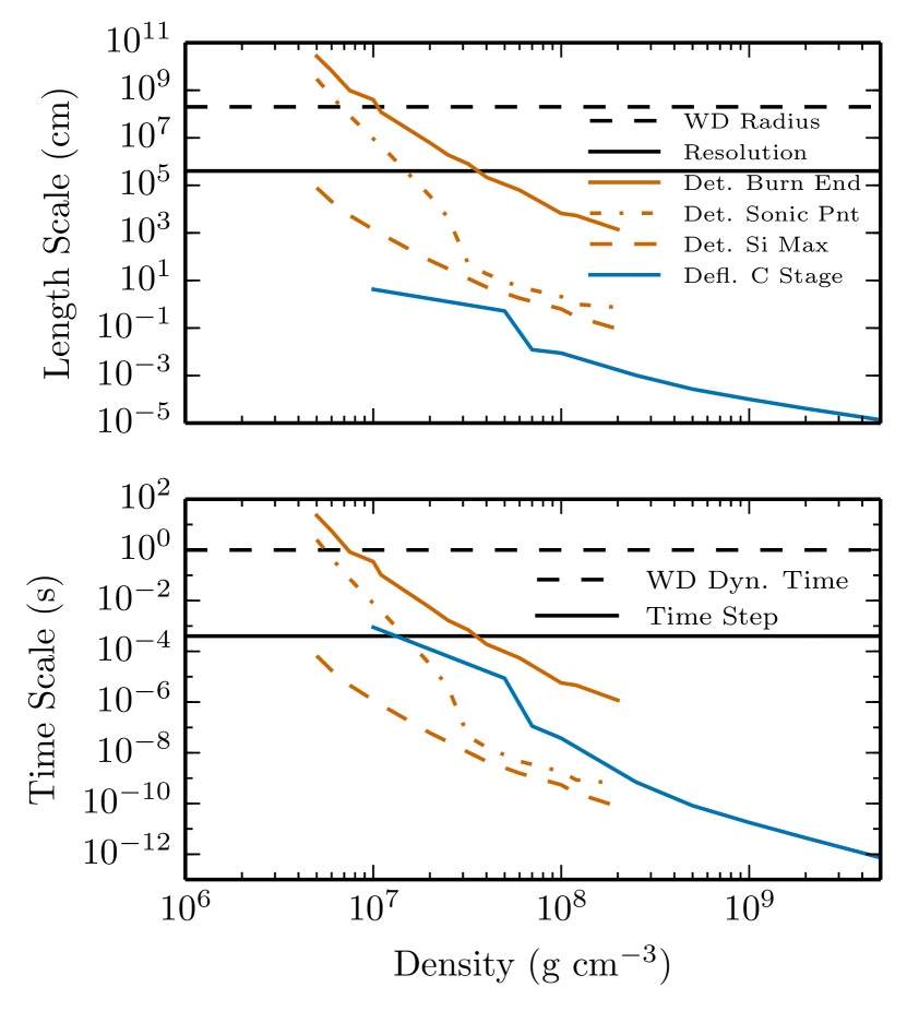
Figure 1.— Length and time scales of burning processes as a function of fuel density for a mixture of ¹²C:¹⁶O:²²Ne in the proportion 50:48:2 compared to typical simulation resolution (4km, solid black lines) and scales of the star (dashed black lines). Stellar scales are taken to be the radius of the initial star and the dynamical time. The top panel shows the size scale of various reaction front features while the bottom shows the self-crossing time of these features at the propagation speed of the reaction front. The behavior of the ¹²C flame is shown by the solid blue curve that extends to high density (Chamulak et al., 2007). Scales for planar steady-state detonations are shown in red. We show the distance from the shock to three points in the detonation structure: the peak of ²⁸Si abundance (dashed), which is also the end of ¹⁶O consumption; the sonic point (dash-dot), also called the pathological point, which is also the size of the detonation driving region; and the attainment of the fully burned NSE state (solid), which is the completion of consumption of ²⁸Si. The detonation driving region transitions from being just resolved to being larger than the radius of the star between densities of about $1.5\times 10^{7}$ g cm^-3 and $7\times 10^{6}$ g cm^-3.

A major challenge in simulations of SNe Ia is capturing these burning processes with confidence and accuracy. The carbon-oxygen reaction fronts transition from being unresolved by many orders of magnitude, to being partially resolved, to finally being larger than the time and length scales of the star. Figure 1 shows length and time scales for detonations (red) and deflagrations (blue, Chamulak et al. 2007) at various densities. For the stellar scales we take the initial WD radius, $R=2\times 10^{8}$ cm, and the dynamical time $2\pi\sqrt{R^{3}/GM}\approx 1$ s where $M$ is the WD mass. A representative simulation resolution of 4 km is shown, along with the corresponding timestep of approximately the sound crossing time of a cell. This resolution was found by Townsley et al. (2009) to be sufficient to give convergence in 1D with the thickened flame reaction front. As a result our multi-dimensional (multi-D) simulations are commonly performed between 4 and 1 km to study resolution dependence in a regime in which convergence is demonstrated in 1D. Several different stages within a steady-state planar detonation front are indicated, with distances measured from the shock that initiates the reactions and propagates the front. The shortest length scale shown (dashed line) is that when the ²⁸Si abundance peaks in time, which also corresponds to the completion of ¹⁶O consumption. The next length scale (dot-dashed line) is the size of the detonation driving region, which is the distance to the sonic point. Finally the solid line shows the distance to completion of burning, reaching the Fe-group element (IGE) dominated nuclear statistical equilibrium (NSE) state.

The total yields of the explosion are determined by how and when the reaction fronts stop propagating as well as what portion of the burning occurs within the reaction front as opposed to what occurs after the reaction front itself has passed. The latter can then be influenced by the expansion of the star. The fairly thin range of densities, $1.5>\rho_{7}>0.7$, $\rho_{7}$ being density in units of $10^{7}$ g cm^-3, in which the detonation driving region transitions from being unresolved to being larger than the radius of the star is a manifestation of the difficulty of capturing the reaction dynamics appropriately. As the driving time and length scales get large, the detonation may not be able to attain the planar steady-state structure. Curvature of the front on scales comparable to the driving length, which will occur due to the structure of the star, reduce the detonation speed and the completeness of the burning (Sharpe, 2001; Dunkley et al., 2013). The long reaction times also mean that an ignited detonation may not reach steady state before the star expands (Townsley et al., 2012).

Many recent results on multi-D simulations of SNe Ia have computed nucleosynthetic yields by post-processing the density and temperature recorded by a Lagrangian fluid history during the simulation (e.g. Travaglio et al., 2004). A large nuclear reaction network is used to integrate a set of species subject to this $\rho(t)$, $T(t)$ history. The burning model used in the simulation is therefore critical, as it determines these histories. Recent multi-D work (Maeda et al., 2010; Seitenzahl et al., 2010; Ciaraldi-Schoolmann et al., 2013; Seitenzahl et al., 2013) has used the method described in the appendix of Fink et al. (2010) to set the energetics of the burning model used in the hydrodynamics. In this technique, the results of the post-processing are used to revise the output of the model of burning and the process is iterated until the yields no longer change.

In this work we pursue a different route toward construction of our burning model and post-processing methods which, instead of an iterative bootstrap, is based on comparison to separate resolved calculations of the deflagration and detonation modes. The burning model and post-processing method are then constructed with the goal that the post-processed results reproduce the results of resolved calculations of the steady-state structure of the reaction front even though the actual reaction front is unresolved. The resolved calculations to which we want to compare are standard methods (e.g. Fickett & Davis, 1979) for the computation of reaction front structure that can be performed with fairly complete nuclear reaction networks and using error-controlled time integration methods to eliminate most computational uncertainty. Here we succeed in matching steady-state yields for detonations at high densities and in planar geometry. Further development of benchmarks and methods for lower densities and other geometries in future work will enable confident higher-accuracy yields for an even larger fraction of the ejecta.

The burning model presented here is the successor to that initially presented by Calder et al. (2007) and Townsley et al. (2007), with tabulations presented by Seitenzahl et al. (2009b), that has been used in a number of studies using large multi-D simulations of SN Ia (Jordan et al., 2008; Meakin et al., 2009; Jordan et al., 2012b, a; Kim et al., 2013; Long et al., 2014). The capability to treat neutron-enriched fuel was added by Townsley et al. (2009) in order to study how neutron enrichment in the progenitor might influence the explosion. The model presented here includes a change in dynamics to better match iron-group production in detonations and extends the treatment of initial composition to spatially non-uniform abundances, allowing more realistic WD progenitors. This has been used in work exploring systematic effects of progenitor WD composition and central density in the DDT scenario, (Krueger et al., 2010; Jackson et al., 2010; Krueger et al., 2012), as well as a study of the turbulence-flame interaction during the deflagration phase (Jackson et al., 2014), and consideration of hybrid C-O-Ne progenitor WDs (Willcox et al., 2016). Those studies, however, did not proceed to nucleosynthetic post-processing, which is discussed in detail here for the first time for our burning model. The first work utilizing the post-processing for astrophysical study is an investigation of spectral indicators of progenitor metallicity (Miles et al., 2015).

We present below the structure of our burning model and post-processing methods, along with particular assumptions currently in use in our SN Ia simulations, as well as tests performed so far comparing to calculations of steady-state deflagrations and detonations. Our burning model is based on tabulation of physical quantities and fits of parameters based on resolved steady-state calculations. To improve accuracy in post-processing, we explore supplementing the Lagrangian $\rho$-$T$ history recorded during the hydrodynamic simulation with a reconstruction of unresolved processes based on conditions near the reaction front when the fluid element is burned.

In section 2 we present the structure of our model for carbon-oxygen burning including the basic variables and the form of their dynamics. Following this, we discuss our post processing treatment for tracks (fluid elements) burned by the deflagration front in section 3. This section is fairly brief since the application of a burning model like that presented here to deflagrations was a major topic of previous work detailed by Calder et al. (2007) and Townsley et al. (2007). Detonations are discussed in two sections. Section 4 develops the error-controlled computation of steady-state detonation structure that we use as a benchmark, calibrates the timescales in the burning model dynamics based on this, and compares the resulting dynamics of the burning model in hydrodynamic tests to the benchmark calculations. The full method including track post-processing is then outlined and tested in section 5. Finally in section 6 we detail how results from full-star simulations are post-processed, and in section 7 we show the results of applying these methods to compute the yields of a 2D simulation of the DDT model of SN Ia, including a consideration of what we can infer about current uncertainties. We summarize conclusions in section 8.

2. Improved Parameterized Model for Explosive Carbon-Oxygen Fusion

We present here our current parameterized model for the thermonuclear burning of carbon and oxygen fuel. The model is intended to capture the dynamics of burning for densities relevant to SNe Ia for either the deflagration or detonation mode of combustion. Conversion of protons to neutrons (neutronization or deleptonization) is included. The initial abundance of carbon and neutron-rich elements (e.g., ²²Ne) are allowed to vary with position in the WD. The model is constructed to use a small number of scalars to track the reaction state and products in order to improve computational efficiency. Accurate final-state energy release and electron capture rates are obtained by tabulation. Abundances of intermediate burning stages are approximated and the formalism can be further refined by adjusting these if necessary.

The process of explosive carbon-oxygen fusion can be roughly divided into 3 stages – C consumption, O consumption, and conversion of Si-group to Fe-group material (Khokhlov, 1989, 2000; Calder et al., 2007). The main processes involved in each of these stages are: C destroyed to produce additional O, Si, Ne, and Mg; O destroyed to produce Si, S, Ar, and Ca, generally in nuclear quasi statistical equilibrium (QSE, sometimes called NSQE); $\alpha$ particles liberated by photodisintegration are then captured until this material is converted into Fe-group, eventually reaching full nuclear statistical equilibrium (NSE). Due to differences in the rates of the nuclear processes involved, at densities of interest these stages are well-separated, in logarithmic time, and sequential. This structure makes it possibly to greatly simplify the complex reaction state and dynamics to the behavior of a model containing just a few reaction progress variables.

Individual cells are allowed to contain both unburned and fully burned material in order to allow modeling of reaction fronts that are much thinner than the grid scale. This conceptual structure is shown in Figure 2, where curves are shown to represent two distinct processes in the overall burn which occur on different timescales. In this example we will use O consumption as the shorter-timescale process and Si consumption as the longer-timescale one. The curves indicate the contour on which the O abundance reaches half of its value in the fuel (solid) and where the Ni abundance reaches half its final value (dashed). Intermediate Ni abundances are represented by dotted lines, which would not be distinct at high densities (the separation between stages is exaggerated at high density). At high densities all reaction stages are localized on scales much smaller than the grid, as indicated by the reaction length scales shown in Figure 1, leading to cells which are volumetrically divided into fuel and ash. At lower densities, some burning stages become resolvable, while others remain thin compared to the grid. For resolvable stages, the actual abundance structure more closely resembles a spatial interpolation of the coarse grid values. This is demonstrated in the lower panel of Figure 2. A structure like this is present for both detonation and deflagration combustion modes, though in the turbulent deflagration phase the thin reaction front structure can me much more irregular than shown in this diagram.

Figure 2.— Diagram of structure of thin, multistage reaction fronts embedded in a coarse computational grid of control volume cells. At high densities the reaction front is completely localized – spatially thin – such that a mixed computational cell contains physically separated regions of fuel and ash material. At lower densities, some reaction stages remain localized, while others extend over multiple cells, so that the reactant and product abundances are smoothly varying on subgrid scales.

Our burning model is currently implemented in the Flash code, an adaptive-mesh reactive hydrodynamics code with additional physics for astrophysical applications developed at the University of Chicago (Fryxell et al., 2000; Dubey et al., 2009). The model is readily adaptable for use with other similar reactive hydrodynamics software and the source code is available as add-on Units for the Flash code, distributed separately to allow a more liberal license.

2.1. Definition of Stages and Relation to Fluid Properties

The first step in abstraction of the fusion processes is defining the relation of our progress variables to the actual physical properties of the fluid. The transformations taking place via nuclear reactions act most fundamentally on the abundances in the fluid. Since we will reduce the burning processes to just a few stages, we must define first how these stages are related to the actual abundances. After this we will proceed to develop reaction kinetics that will reproduce the effects that the nuclear reactions have on the actual abundances and how that manifests in the corresponding abstracted stages.

Our basic physics will be phrased in terms of baryon fractions, denoted by the symbol $X_{i}$. These are the fraction of the total number of baryons which are in the form of the nuclide indicated by the label $i$. This is very similar to the traditional definition of mass fractions, but avoids the ambiguity that rest mass is not conserved as nuclear reactions take place due to energy release. Since Baryon number is a conserved quantity, in the absence of sources the baryon number density, $n_{B}$, satisfies the continuity equation:

$$\frac{\partial(n_{B})}{\partial t}=-\vec{\nabla}\cdot(n_{B}\vec{v})\ ,$$ (1)

where $\vec{v}$ is the fluid velocity. For reasons of convenience in a non-relativistic fluid code, we will make the definition

$$\rho\equiv m_{u}n_{B}\,[=]\,n_{B}/N_{A}\ ,$$ (2)

where $m_{u}$ is the atomic mass unit and $N_{A}$ is Avogadro’s number. Here $[=]$ is used to denote ”is numerically equivalent to in cgs units.” Our intention is to place distinction between mass and (binding) energy in the gravitational treatment; we could calculate the mass-energy density if necessary, but computation of gravity in our simulation will just use $\rho$ to approximate it. The baryon fractions $X_{i}$ then identify directly the number of baryons in species $i$ and therefore, in the absence of reactions, also follow a conservation equation of the form

$$\frac{\partial(Xn_{B})}{\partial t}=-\vec{\nabla}\cdot(Xn_{B}\vec{v})\ .$$ (3)

Where $X$ may be $X_{i}$ or one of the progress variable defined below that will be constructed as linear combinations of the $X_{i}$. Taken together Equation (3) and Equation (2) mean that any linear combination of baryon fractions can be treated as “mass scalars” by the advection infrastructure in conservative fluid dynamics software (e.g. Flash; Fryxell et al. 2000; Dubey et al. 2009).

In order to start from quantities that satisfy Equation (1), for purposes of tracking 3 stages of burning (that is three transitions), we conceive of having four sets of all nuclides, each of which represents a certain ”type” of material:

$$X_{f,i},\quad X_{a,i},\quad X_{q,i},\quad X_{N,i}\ ,\quad\quad\sum_{\alpha,i}X_{\rm\alpha,i}=1\ .$$

These denote, respectively, the baryon fractions of individual species comprising fuel, (intermediate) ash (product of carbon consumption), a quasi-equilibrium (QSE) group, and a terminal (NSE) group. These stages and the various symbols used here are laid out in the diagram in Figure 3. This means that any given baryon has two labels: the type of nucleus in which it resides (e.g. silicon), and whether we call that material part of, for example, the ash or the QSE material. It is convenient to define 4 “superspecies” by

$$\mathcal{X}_{\alpha}=\sum_{i}X_{\alpha,i}\quad\alpha=\{f,a,q,N\}\ .$$ (4)

Figure 3.— Diagram of burning stages for C+O burning and associated symbols used here. The progress of burning of a fluid element is from left to right, with the horizontal axis indicating distance with respect to the foremost part of the reaction front or time as a fluid element passes through the reaction front. See section 4.3 for comparison to an actual reaction front structure.

Since each of the burning stages follows in sequence from the earlier ones – a feature unlike general nuclear species in a reaction network – it is convenient to define progress variables such that

$$\mathcal{X}_{f}=1-\phi_{fa}\ ,\ \mathcal{X}_{a}=\phi_{fa}-\phi_{aq}\ ,\ \mathcal{X}_{q}=\phi_{aq}-\phi_{qn}\ ,\ \mathcal{X}_{N}=\phi_{qn}\ ,$$ (5)

or

$$\phi_{fa}=\mathcal{X}_{a}+\mathcal{X}_{q}+\mathcal{X}_{N}\ ,\quad\phi_{aq}=\mathcal{X}_{q}+\mathcal{X}_{N}\ ,\quad\phi_{qn}=\mathcal{X}_{N}\ .$$ (6)

By virtue of the property $0\leq X_{\alpha,i}\leq 1$ and thus $0\leq\mathcal{X}_{\alpha}\leq 1$, we see that $1\geq\phi_{fa}\geq\phi_{aq}\geq\phi_{qn}\geq 0$. Also, since the $\phi_{\alpha\beta}$ are simply linear combinations of the $X_{\alpha,i}$ they also satisfy continuity, Equation (1), in the absence of sources.

We define a set of specific abundances:

$$\xi_{\alpha,i}\equiv\frac{X_{\alpha,i}}{\mathcal{X}_{\alpha}}\,\quad\alpha=\{f,a,q,N\}\ ,$$ (7)

so that $\sum_{i}\xi_{\alpha,i}=1$. This is useful because we will, at times, want to specify $X_{\alpha,i}=\mathcal{X}_{\alpha}\xi_{\alpha,i}$ by specifying $\xi_{\alpha,i}$. This subtle distinction was left unaddressed in our previous revisions of this burning model (Calder et al., 2007; Townsley et al., 2007). Note that since the $\xi_{\alpha,i}$ are quotients of the $X_{\alpha,i}$, they are no longer linear combinations. Nonlinear terms are any that contain products or quotients of fields that are position-dependent. Linear combinations are required in order for the numerical scheme to be explicitly conservative. While any general algebraic combination, including a nonlinear one like a product or power, of quantities satisfying Equation (1) still satisfies Equation (1), once the fields $\rho$, $X$, and $\xi$ are discretized into values averaged over control volumes, i.e., mesh cells, conservation of $X$’s no longer implies conservation of $\xi$’s due to nonlinearities in the advection scheme. This results from the property that the average of a quotient is not the quotient of the averages. Since we will not compute Equation (1) for both the $X$’s and $\xi$’s, we must make a choice of which will satisfy explicit conservation to numerical accuracy, as performed by a conservative advection scheme like that in Flash. Since overall energy release is important, we choose to compute conservative evolution for quantities that are linear combinations of the $X$’s.

In order to evaluate fluid properties and follow nuclear energy release into the fluid, we must be able to obtain several bulk quantities. We will express these in units per baryon, such that obtaining units per cm³ is trivial using the Baryon density $n_{B}\equiv\rho/m_{u}$. The two fluid quantities necessary are:

$$\text{Numberofprotonsperbaryon:}\quad Y_{p}=Y_{e}\equiv\sum_{\alpha,i}X_{\alpha,i}\frac{Z_{i}}{A_{i}}$$ (8)

$$\text{Numberofionsperbaryon:}\quad Y_{\rm ion}\equiv\sum_{\alpha,i}X_{\alpha,i}\frac{1}{A_{i}}\ ,$$ (9)

where, as customary, $Z_{i}$ is the number of protons and $A_{i}$ is the number of protons plus neutrons in nuclide $i$. Here we have assumed charge neutrality between the number of protons and the number of non-thermal electrons, and defined $Y_{e}$ to include only the net non-thermal electrons. Some $e^{+}$-$e^{-}$ pairs are created thermally at high temperatures and these are accounted for in the EOS (Timmes & Arnett, 1999), and therefore are, in effect, advected with the energy field instead of as fluid electrons included in our definition of $Y_{e}$.

For energetic purposes we need to be able to track the rest-mass of our material rather than the approximation mentioned above. This is accomplished by tracking the nuclear binding energy per baryon:

$$\bar{q}\equiv\sum_{\alpha,i}X_{\alpha,i}\frac{Q_{i}}{A_{i}}=\sum_{\alpha,i}\frac{X_{\alpha,i}}{A_{i}}\left[Z_{i}m_{p}+N_{i}m_{n}-m_{i}\right]c^{2}\ ,$$ (10)

where $m_{p}$ and $m_{n}$ are the masses of the (free) proton and neutron respectively and $m_{i}$ is the mass of 1 nucleus of nuclide $i$. Note that $m_{i}$ is not the atomic mass, which is often given in mass tables and includes electrons and their binding energy. The average mass of a baryon in the fluid is

$$\bar{m}_{B}=\sum_{\alpha,i}X_{\alpha,i}\frac{m_{i}}{A_{i}}=[m_{n}+Y_{e}(m_{p}-m_{n})]c^{2}-\bar{q}\ .$$ (11)

Thus the actual rest mass density is $\rho_{\rm rest}=\bar{m}_{B}n_{B}=\rho\bar{m}_{B}/m_{u}$. Note that because the nuclear binding energy, $\bar{q}$, is defined with respect to free protons and neutrons in the same proportion as the material, calculation of the average rest mass requires both $\bar{q}$ and $Y_{e}$, with the latter specifying the overall relative numbers of protons and neutrons in the material.

We may now define the group-specific quantities

$$Y_{e,\alpha}=\sum_{i}\xi_{\alpha,i}\frac{Z_{i}}{A_{i}}\ ,\ Y_{{\rm ion},\alpha}=\sum_{i}\xi_{\alpha,i}\frac{1}{A_{i}}\ ,\ \bar{q}_{\alpha}=\sum_{i}\xi_{\alpha,i}\frac{Q_{i}}{A_{i}}\ .$$ (12)

so that

$$Y_{e}=\sum_{\alpha}\mathcal{X}_{\alpha}Y_{e,\alpha}\ ,\ Y_{\rm ion}=\sum_{\alpha}\mathcal{X}_{\alpha}Y_{{\rm ion},\alpha}\ ,\ \bar{q}=\sum_{\alpha}\mathcal{X}_{\alpha}\bar{q}_{\alpha}\ .$$ (13)

It is again important to note that the group-specific quantities such as $\bar{q}_{\alpha}$ are not linear combinations of the $X_{\alpha,i}$ because the $\xi_{\alpha,i}$ are quotients of linear combinations of the $X_{\alpha,i}$. In order to maintain machine-precision advection of the discretized field $Y_{e}$, for example, we will need to perform a conservative advection scheme on the product $\mathcal{X}_{\alpha}Y_{e,\alpha}$ instead of separately on $\mathcal{X}_{\alpha}$ and $Y_{e,\alpha}$, since their product will not evolve conservatively to machine precision. A similar statement holds for $Y_{\rm ion}$ and $\bar{q}$.

We will derive the quantities $Y_{e,f}$, $Y_{{\rm ion},f}$, $\bar{q}_{f}$, and $Y_{e,a}$, $Y_{{\rm ion},a}$, $\bar{q}_{a}$ from the initial state. Our simulation begins with fuel of known abundances,

$$X_{0,i}(\vec{x}),\quad\sum_{i}X_{0,i}=1\ ,$$ (14)

which may vary in space as indicated. These initial abundance will satisfy Equation (1) throughout our simulation; they will have no sources. This allows us to, throughout the burning process, know how much of the local baryons were in what form initially. From these we define the properties of the fuel,

$$Y_{e,f}(\{X_{0,j}\}) = \sum_{j}X_{0,j}\frac{Z_{j}}{A_{j}}\ ,$$

$$Y_{{\rm ion},f}(\{X_{0,j}\}) = \sum_{j}X_{0,j}\frac{1}{A_{j}}\ ,$$ (15)

$$\bar{q}_{f}(\{X_{0,j}\}) = \sum_{j}X_{0,j}\frac{Q_{j}}{A_{j}}\ .$$

Additionally the ashes of the first stage of burning are assumed to be only a function of the initial composition. Thus

$$\xi_{a,i}=\xi_{a,i}(\{X_{0,j}\})$$

and is therefore also position dependent. Then

$$Y_{e,a}(\{X_{0,j}\}) = \sum_{i}\xi_{a,i}(\{X_{0,j}\})\frac{Z_{i}}{A_{i}}\ ,$$

$$Y_{{\rm ion},a}(\{X_{0,j}\}) = \sum_{i}\xi_{a,i}(\{X_{0,j}\})\frac{1}{A_{i}}\ ,$$ (16)

$$\bar{q}_{a}(\{X_{0,j}\}) = \sum_{i}\xi_{a,i}(\{X_{0,j}\})\frac{Q_{i}}{A_{i}}\ .$$

As an aside, some concrete examples are useful. In the Townsley et al. (2007) burning model, the initial abundances were $\{X_{0,^{12}\rm C}=0.5,\ X_{0,^{16}\rm O}=0.5\}$, constant in space, and with other abundances zero. Also the ashes of carbon consumption were specified by $\xi_{a,^{16}\rm O}=X_{0,^{16}\rm O}$ and $\xi_{a,^{24}\rm Mg}=X_{0,^{12}\rm C}$, with others again zero. In Townsley et al. (2009) the abundances of the fuel and carbon-consumption ash stages were effectively modified to add a small amount of ²²Ne, whose abundance was still uniform in space, so that the initial abundances were $\{X_{0,^{12}\rm C}=0.5,\ X_{0,^{16}\rm O}=0.48,\ X_{0,^{22}\rm Ne}=0.02\}$, constant in space, and carbon-consumption ash abundances were {$\xi_{a,^{16}\rm O}=X_{0,^{16}\rm O},\ \xi_{a,^{24}\rm Mg}=X_{0,^{12}\rm C},\ \xi_{a,^{22}\rm Ne}=X_{0,^{22}\rm Ne}\}$. In the model at hand we will use two parameters $X_{0,^{12}\rm C}$ and $X_{0,^{22}\rm Ne}$ that vary in space to define the initial state, and the $\xi_{a,i}$ are defined as previously. More detailed fuel abundances, or those containing additional major constituents such as ²⁰Ne or ²⁴Mg also fit naturally into this scheme.

The fluid properties of the fuel and ashes of just the carbon burning step depend almost entirely on the initial abundances. For the equilibrium groups (QSE and NSE), however, all of these properties change dynamically as the nuclear processing continues at high temperatures. The broad rearrangements of abundances which lead to the variation of properties like $Y_{\rm ion}$ and $\bar{q}$ in the more processed ashes are precisely the dynamics that we would like to abstract down to a few parameters for the sake of computational efficiency. To this end, we will treat gross properties of the quasi-equilibrium and equilibrium groups together. For convenience we define another superabundance representing the total amount of material in either QSE or NSE, $\mathcal{X}_{qn}=\mathcal{X}_{q}+\mathcal{X}_{N}=\phi_{aq}$. This allows us to collect the properties of the equilibrium groups by defining:

$$\delta Y_{e,qn} \equiv \mathcal{X}_{qn}Y_{e,qn}$$ (17)

$$\delta Y_{{\rm ion},qn} \equiv \mathcal{X}_{qn}Y_{{\rm ion},qn}$$ (18)

$$\delta\bar{q}_{qn} \equiv \mathcal{X}_{qn}\bar{q}_{qn}$$ (19)

The $\delta$ prepended to the quantities here helps to indicate the somewhat odd units involved. For example, $\delta Y_{{\rm ion},qn}$ is the number of QSE+NSE ions (nuclei) per fluid Baryon, whereas $Y_{{\rm ion},qn}$ itself is the number of QSE+NSE ions per QSE+NSE Baryon. This unit convention is the most awkward for $\delta\bar{q}_{qn}$. To restate why this is desirable: If we had chosen instead to treat $\bar{q}_{qn}$ directly, that would cause the total nuclear energy $\bar{q}=\mathcal{X}_{f}\bar{q}_{f}+\mathcal{X}_{a}\bar{q}_{a}+\mathcal{X}_{qn}\bar{q}_{qn}$, which is a nonlinear combination of $\mathcal{X}_{qn}$ and $\bar{q}_{qn}$, to not be explicitly conserved by the conservative hydrodynamics scheme. Applying the conservative hydrodynamics to $\delta\bar{q}_{qn}$ maintains conservation of the total nuclear energy. This form also makes it straightforward to derive appropriate dynamics, which we do below.

Using the progress variables, intermediate state definitions, and QSE+NSE material definitions, the bulk fluid properties can be restated as

$$Y_{e} = [1-\phi_{fa}]Y_{e,f}(\{X_{0,j}\})$$ (20)

$$\mbox{}+[\phi_{fa}-\phi_{aq}]Y_{e,a}(\{X_{0,j}\})+\delta Y_{e,qn}$$

$$Y_{\rm ion} = [1-\phi_{fa}]Y_{{\rm ion},f}(\{X_{0,j}\})$$ (21)

$$\mbox{}+[\phi_{fa}-\phi_{aq}]Y_{{\rm ion},a}(\{X_{0,j}\})+\delta Y_{{\rm ion},qn}$$

$$\bar{q} = [1-\phi_{fa}]\bar{q}_{f}(\{X_{0,j}\})$$ (22)

$$\mbox{}+[\phi_{fa}-\phi_{aq}]\bar{q}_{a}(\{X_{0,j}\})+\delta\bar{q}_{qn}\ .$$

This defines the relationship of our burning model variables to the physical fluid properties.

2.2. Posited source terms

The previous subsection developed a framework in which the properties of the parameterized burning stages can be expressed in a way that can be advected in the absence of sources. This leaves us to define dynamical equations (source terms) for the $\phi_{\alpha\beta}$ themselves and the properties of the equilibrium materials (the $\delta$ prefixed quantities). By specifying these source terms here, we complete the form of the burning model.

First a brief note on the form of the source terms which we will posit. Typically we will write down source terms by specifying the Lagrangian time derivative

$$\frac{DX}{Dt}=\frac{\partial X}{\partial t}+\vec{v}\cdot\nabla X\ .$$ (23)

In Eulerian form this gives

$$\frac{\partial(X\rho)}{\partial t}=-\vec{\nabla}\cdot(X\rho\vec{v})+\rho\frac{DX}{Dt}\ .$$ (24)

Thus we are specifying the term in the evolution of the conserved quantity that is due to transformations rather than just advection.

The evolution of the first stage of burning, $\phi_{fa}$, can be set from a flame-tracking scheme or via a thermal reaction rate. This is done just as it is in Townsley et al. (2009),

$$\frac{D\phi_{fa}}{Dt}=\max(0,\dot{\phi}_{\rm RD})+\dot{\phi}_{\rm CC}\ ,$$ (25)

where $\dot{\phi}_{\rm RD}$ is the reaction due to the reaction-diffusion (RD) flame propagation calculation, and $\dot{\phi}_{\rm CC}$ is thermally activated carbon-carbon fusion (Townsley et al., 2009). The other progress variables then obey

$$\frac{D\phi_{aq}}{Dt} = \frac{\phi_{fa}-\phi_{aq}}{\tau_{NSQE}(T)}\ ,$$ (26)

$$\frac{D\phi_{qn}}{Dt} = \frac{(\phi_{aq}-\phi_{qn})^{2}}{\tau_{NSE}(T)}\ .$$ (27)

Here the $\tau_{NSQE}$ is the timescale previously determined in Calder et al. (2007) for oxygen consumption. $\phi_{aq}$ reaches completion at the peak Si abundance, when all oxygen is consumed. The time and length scales for completion of this stage were given as the dashed lines in Figure 1. As can be seen there, this stage is mostly unresolved in our simulations for steady-state detonations, including at all densities important for Fe-group production, where the scales for completion of burning are less than the stellar scales.

In contrast, as shown by the solid lines in Figure 1, the completion of processing of Si- to Fe-group, the $\phi_{qn}$ phase, can occur on resolved scales for $\rho\lesssim 3\times 10^{7}$ g cm^-3. Additionally, this stage can be left incomplete for $\rho\lesssim 10^{7}$ g cm^-3 by the limited length scales in the star and time of expansion of the star. Therefore, the dynamics of this phase are very important for accurate total Fe-group yields. The dynamics we are now using for $\phi_{qn}$, Equation (27), differs from that used previously (Townsley et al., 2009; Jordan et al., 2008; Meakin et al., 2009; Jordan et al., 2012b, a; Kim et al., 2013; Long et al., 2014), $D\phi_{qn}/Dt=(\phi_{aq}-\phi_{qn})/\tau_{\rm NSE}$. In the process of performing the comparisons to benchmark detonation abundance structures presented in section 4.3, it was found that the dynamics used previously led to an approximately exponential relaxation of $\phi_{qn}$ that did not match the time dependence of the consumption of Si as well as was hoped. In order to improve accuracy of our recorded Lagrangian histories, the dynamics applied to $\phi_{qn}$ was altered to that of Equation (27). This also necessitates recalibration of the parameter $\tau_{\rm NSE}$, which will be performed below in section 4.2.

Both of the parameterized timescales above, $\tau_{\rm NSQE}$ and $\tau_{\rm NSE}$, depend on temperature, $T$, and some of the values used below also depend on density. However, there will be significant regions in the artificial flame reaction front – where $\phi_{\rm RD}$ is not near 0 or 1 – that have a cell-averaged temperature and density that is not a good representation of the temperature of most of the fluid in the cell. These are regions where, as shown in Figure 2, a cell at the reaction front in reality consists partly of unburned fuel and partly of fully burned material separated by a thin front. In this region our use of an artificially thickened reaction front gives a temperature intermediate between that of the fuel and ash. The evaluation of the timescales also needs to be stable as $\phi_{\rm RD}$ changes to obtain reasonable burning dynamics. By assuming the rest of the burning will occur at either constant density or constant pressure, the final burned state, $\rho_{f}$, $T_{f}$, and abundances can be determined based on the current local abundances and thermal state (Calder et al., 2007). The constant pressure prediction provides a reasonable approximation for the final burning state that will be reached by the flame, and so the $\rho_{f}$ and $T_{f}$ of this final state are used to evaluate $\tau_{\rm NSQE}$, $\tau_{\rm NSE}$, $\bar{q}_{\rm NSE}$, $Y_{\rm ion,NSE}$, and $\dot{Y}_{e,\rm NSE}$ (see below) in regions were $10^{-6}<\phi_{\rm RD}<0.99$. Otherwise, in regions away from the artificial flame the local temperature is used to evaluate $\tau_{\rm NSE}$ and the temperature predicted for an isochoric evolution is used to evaluate $\tau_{\rm NSQE}$, $\bar{q}_{\rm NSE}$, $Y_{\rm ion,NSE}$, and $\dot{Y}_{e,\rm NSE}$.

Evolution of $Y_{e}$ due to electron capture occurs mainly by conversion of Fe-group material, that is material that has at some point fully relaxed to NSE. At the densities relevant to our SNIa computation, the timescale for relaxation to NSE and the timescale for electron capture are well enough separated that electron capture in material that is only partially fully relaxed to NSE is not an issue. However, due to the artificially thickened reaction front in our SN Ia simulations, a single cell at high densities will consist of an artificial mixture of unburned fuel and fully relaxed NSE ash undergoing electron capture. To constrain electron capture evolution to relaxed NSE material, we separate the components of $Y_{e}$ further into QSE and NSE portions:

$$\delta Y_{e,qn}=\delta Y_{e,q}+\delta Y_{e,N}=\mathcal{X}_{q}Y_{e,q}+\mathcal{X}_{N}Y_{e,n}\ .$$ (28)

For all but the NSE material, $Y_{e,f}=Y_{e,a}=Y_{e,q}=Y_{e,0}\equiv Y_{e}(\{X_{0,i}\})$. This simplifies Equation (20) to

$$Y_{e}=(1-\phi_{qn})Y_{e,0}+\delta Y_{e,n}\ .$$ (29)

Applying the chain rule to $\delta Y_{e,n}$ gives

$$\frac{D(\delta Y_{e,n})}{Dt}=\frac{D\mathcal{X}_{N}}{Dt}Y_{e,n}+\mathcal{X}_{N}\frac{DY_{e,n}}{Dt}\ .$$ (30)

The right hand side terms each have a distinct physical interpretation. The first is the change due to newly produced material, while the second is due to the adjustment of the pre-existing material. New NSE material is created with $Y_{e,0}$ and old NSE material evolves according to the tabulated $\dot{Y}_{e,\rm NSE}$, which naturally gets scaled by the fraction of material currently fully relaxed to NSE, $\mathcal{X}_{N}\equiv\phi_{qn}$, so that

$$\frac{D(\delta Y_{e,n})}{Dt}=\frac{D\phi_{qn}}{Dt}Y_{e,0}+\phi_{qn}\dot{Y}_{e,\rm NSE}\ .$$ (31)

Next we consider $\delta\bar{q}_{qn}$. This represents the average binding energy of all material involved in incomplete Si burning, whether currently in QSE or having progressed fully to NSE. Using the chain rule on Equation (19) splits this into two contributions,

$$\frac{D(\delta\bar{q}_{qn})}{Dt} = \frac{D(\phi_{aq})}{Dt}\bar{q}_{qn}+\phi_{aq}\frac{D(\bar{q}_{qn})}{Dt}\ .$$ (32)

In earlier versions (Townsley et al. 2009 and prior) of this burning model, we posited dynamics in which the binding energy relaxed to the NSE value on the shorter relaxation timescale, $\tau_{\rm NSQE}$. However, in verification comparisons to detonation structures it was found that at low densities this released energy too quickly and led to under-prediction of the temperature just behind the unresolved portion of the detonation front. In order to improve this behavior, we here introduce a $\delta\bar{q}_{\rm QSE}$ that changes as Si-group material is converted to Fe-group, as measured by the progress variable $\phi_{\rm qn}$,

$$\delta\bar{q}_{\rm QSE}=(\phi_{aq}-\phi_{qn})\bar{q}_{\rm QSE0}+\phi_{qn}\bar{q}_{\rm NSE}\ .$$ (33)

Relaxation toward this value is assumed to occur via $\alpha$ capture or photodisintegration, and thus take place on the shorter timescale $\tau_{\rm NSQE}$. To capture these two timescales we posit the following dynamics,

$$\frac{D\delta q_{qn}}{Dt} = \frac{D(\phi_{aq})}{Dt}\bar{q}_{\rm QSE0}$$ (34)

$$\mbox{}+\frac{1}{\tau_{\rm NSQE}}\left[(\phi_{aq}-\phi_{qn})\bar{q}_{\rm QSE0}+\phi_{qn}\bar{q}_{NSE}-\delta\bar{q}_{qn}\right]\ ,$$

where the evolution on the timescale $\tau_{NSE}$ is contained in $\phi_{qn}$. Here $\bar{q}_{\rm QSE0}$ represents the $\bar{q}$ of the material at the completion of O consumption, that is the initial QSE state. This state is less easily quantified at high densities, as it may contain a significant, and density-dependent, fraction of $\alpha$ particles, but it will only be important at low densities when the Si burning is resolved in the simulation. While, therefore, the most appropriate value for $\bar{q}_{\rm QSE0}$ is likely to be density- and composition-dependent, for simplicity we will use $\bar{q}_{\rm QSE0}=q_{{}^{28}\rm Si}$, which appears mostly sufficient in the verification tests performed.

The evolution of $Y_{\rm ion}$, or equivalently the ion mean molecular weight, $\bar{A}$, poses a similar challenge to $\bar{q}$. Each of the QSE and NSE materials will relax the balance between heavies and $\alpha$/protons/neutrons on approximately the NSQE relaxation time, whereas the conversion between QSE and NSE occurs more slowly. We resolve this by using the scalar that tracks relaxation toward NSE, $\phi_{qn}$, to appropriately mix approximations of $Y_{\rm ion}$ for the QSE and NSE states and then set our dynamics to move toward this value on the NSQE timescale. Working in a way similar to the construction of Equation (34),

$$\frac{D(\delta Y_{{\rm ion},qn})}{Dt} = \frac{D\phi_{aq}}{Dt}Y_{\rm ion,QSE0}$$

$$\mbox{}+\frac{1}{\tau_{NSQE}}\left[(\phi_{aq}-\phi_{qn})Y_{\rm ion,QSE0}+\phi_{qn}Y_{{\rm ion},NSE}-\delta Y_{{\rm ion},qn}\right]\ .$$

It is left to obtain a suitable estimate of $Y_{{\rm ion},QSE0}$ for the QSE state. We found that at densities $\lesssim 10^{7}$ g cm^-3 that the simple estimate $Y_{\rm ion,QSE0}\equiv Y_{{}^{28}\rm Si}=1/28$ provides a well-behaved approximation that matches $\bar{A}$ produced by benchmark detonation calculations within 10% (see section 4.3). A somewhat complex approximation was proposed in Townsley et al. (2009), but it did not yield a better match to $\bar{A}$ in testing.

The dynamics of our parameterized model for CO burning are contained in Equations (25), (26), (27), (31), (34), and (2.2). The energy release is computed based on conservation of energy, giving the energy release rate per mass,

$$\epsilon_{\rm nuc}=\dot{\bar{q}}-\phi_{\rm qn}[\dot{Y}_{e,\rm NSE}N_{\rm A}c^{2}(m_{p}+m_{e}-m_{n})+\epsilon_{\nu,\rm NSE}]\ ,$$ (36)

where $m_{p}$, $m_{e}$, and $m_{n}$ are the masses of the proton, electron, and neutron respectively, and $\epsilon_{\nu,\rm NSE}$ is the energy loss to emission of neutrinos based on the local predicted NSE abundances. While the burning dynamics has been stated analytically, the resulting differential equations must now be implemented in a way that is numerically efficient. It is possible to exploit some aspects of the separation between timescales and the strict ordering of the burning stages to make the integration of these dynamical equations extremely efficient. This is discussed in Appendix E.

2.3. Calculation of Nucleosynthesis Using Post-Processed Lagrangian particle Histories

The burning model presented here is intended to give approximately the right energy release, as determined by direct computation of steady-state reaction front structure with large, complete nuclear networks and error-controlled numerical methods, but with a relatively low computational cost. In order to recover detailed abundances, Lagrangian fluid histories are recorded from the hydrodynamic simulation and post-processed. Our post-processing is described in later sections.

The Flash code includes the capability to produce Lagrangian fluid histories through the use of ”tracer” particles (Dubey et al., 2012). These are particles whose position is calculated as

$$\vec{x}(t)=\vec{x}_{0}+\int_{t_{0}}^{t}\vec{v}[\vec{x}(t^{\prime}),t^{\prime}]\,dt^{\prime}$$ (37)

Where the time-dependent velocity field $\vec{v}[\vec{x},t]$ is simply that determined by the hydrodynamic evolution. Generally the number of particles followed and the distribution of initial positions $\vec{x}_{0}$ are chosen to provide a sampling that is useful for nucleosynthesis (Seitenzahl et al., 2010), though here we use a simple weighting in which each tracer represents an equal mass and initial positions are chosen randomly to follow the mass distribution. This random distribution is achieved as follows: The domain is decomposed into blocks of $8^{d}$ cells, where $d$ is the dimension, 2 in this case, and we are using blocks that are 8 cells on a side. The mesh structure in Flash provides an ordering for these blocks, called the Morton ordering (Fryxell et al., 2000). We split the mass of the star into segments based on how much mass is contained in each block, using the same order as the Morton ordering. A random number between zero and the total mass is then generated for each particle, and the segment in which it falls determines the block in which that particle is initially placed. A similar procedure is repeated at the block level, using the mass of material in each cell. Once the cell in which the particle will be placed is chosen, each coordinate of the location of the particle within the cell is chosen randomly and uniformly across each dimension of the cell. The impact of the finite sampling represented by this distribution on the uncertainty of our results is discussed in Appendix C.

The Lagrangian tracks are then computed at the same time as the hydrodynamics. The method used to perform the integration of the particle positions is essentially a second-order Runge-Kutta scheme with the velocity field sampled at the end of each combined hydrodynamics and energy source step and linearly interpolated to the particle position. Note that in the directionally-split hydrodynamics solver, which is used here, each hydrodynamics step consists of multiple sweeps of the 1D PPM method to allow for multi-D problems (Fryxell et al., 2000).

3. Deflagration Fronts

Particles representing fluid burned by a deflagration front must be treated differently from those undergoing detonation because the true burning structure differs from the effective one used in the simulation. In some ways treatment of the particles undergoing deflagration is more straightforward because the combustion in the hydrodynamical calculation has been made into a spatially resolved process by coupling it to the RD front as given in Equation (25). The parameterized dynamics used for the RD front are the same as those discussed in Townsley et al. (2009), basically causing the 4-zone wide reaction front to propagate at a specified speed. However, since the flame is generally quite subsonic, with Mach number ${\rm Ma}\ll 0.01$, it will typically take many time-steps, approximately $4/{\rm Ma}$, for a fluid element tracked by a Lagrangian tracer particle to pass fully through the RD front. In our simulations this is several tenths of a second, as can be seen by the progress variable and temperature histories shown by the solid black lines in Figure 4. During this time, by construction (Townsley et al., 2009, and section 2.2 above), the local temperature is not physical, but a mixture between burned and unburned states in approximate pressure equilibrium. This makes it essential to perform a reconstruction of the portion of the particle’s thermodynamic history during which it is still inside the RD front, before the fully burned state is reached.

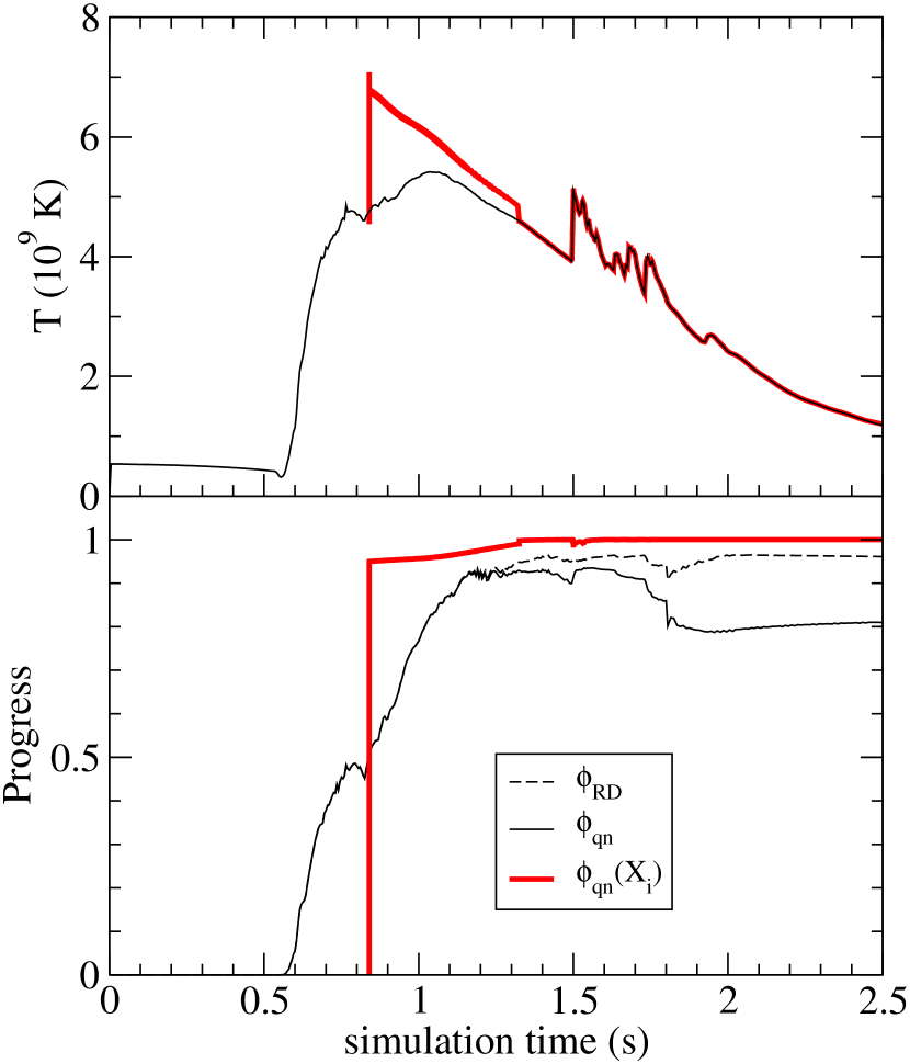
Figure 4.— Thermal and burning progress histories for fluid burned by a deflagration front. Shown is the temperature (upper panel thin solid), reaction-diffusion front progress variable ($\phi_{\rm RD}$, lower panel dashed) and QSE to NSE progress variable ($\phi_{qn}$, lower panel thin solid) recorded at the position of the Lagrangian tracer particle embedded in material ejected at approximately 5 000 km s^-1. $\phi_{\rm RD}$ and $\phi_{qn}$ are identical up to about 1.2 s, at which time the fluid element reaches low enough temperature and density that the separation between burning stages begins to become spatially resolvable. Also shown (thick red solid lines) are the reconstructed temperature history used in the post-processing calculation of nucleosynthetic yields and an analog of $\phi_{\rm qn}$ constructed from the detailed abundances, $X_{i}$, computed during post processing (see Equation 38).

The black line in the upper panel of Figure 4 shows a typical temperature history for a tracer particle embedded in material ejected in a DDT SNIa at approximately $5\,000$ km s^-1. The bottom panel shows the evolution of the progress variable representing relaxation toward Fe-group, $\phi_{\rm qn}$ (solid black line). As can be seen, the transition from unburned to nearly fully burned covers times from about 0.6 s to 1.2 s, and the slow rise in temperature seen in the upper panel covers a similar time range. During this interval, the density and temperature are not representative of a physical burning process, but are instead the average of the burned and unburned states based on the fraction of the cell burned as indicated by the artificially thickened reaction front (see Figure 2). This makes calculation of, for example, the electron-capture history of this fluid element based on a direct post-processing of the $\rho(t)$, $T(t)$ history inappropriate.

We attempt to reconstruct a reasonable approximation to the temperature-density history that a fluid element would have undergone passing through a flame of realistic thickness. The reconstruction of the portion of the fluid history that elapses while the particle is within the artificially broad reaction region is obtained by assuming that the pressure jump across the flame is small, $\lesssim 1\%$ (Vladimirova et al., 2006; Calder et al., 2007). This will be true as long as the Mach number of the flame propagation is low, as is the case for our simulations. Under this assumption, although the local density and temperature are not representative of the actual values, the local pressure should be similar to that near the actual thin flame front to within approximately the Mach number. In order to use this feature, we perform self-heating calculations with a pressure history specified from the fluid histories extracted from the hydrodynamic simulation. This novel mode of specified-pressure-history self-heating was added to the TORCH nuclear reaction network (Timmes, 1999). The set of 225 nuclides used includes all those indicated in the discussion of weak reactions in Calder et al. (2007), which includes an extension to neutron-rich nuclides near the Fe group compared to the standard 200 nuclide set used in TORCH. Weak cross sections were taken from Fuller et al. (1985), Oda et al. (1994), and Langanke & Martínez-Pinedo (2001), with newer rates superseding earlier ones.

Assuming that the fluid element actually crosses the flame front when the progress variable passes through $\phi_{RD}=0.5$, the reconstructed temperature history is shown by the red curve in the upper panel of Figure 4. It is notable that the temperature peak is much higher and occurs about 0.2 seconds sooner. The initial condition for the trajectory is found by performing a short computation at constant pressure that was raised high enough for the ¹²C to begin burning ($2\times 10^{9}$ K), continuing until the ¹²C abundance is 0.1. The specified-pressure self-heating follows this. Once the fluid element exits the artificial reaction front, post-processing can proceed from there using the recorded temperature-density history. We take this point to be when $\phi_{RD}>0.95$ in the recorded history, or when $P<10^{22}$ erg cm^-3, whichever comes first. This $P$ corresponds roughly to when burning of heavier elements will cease, when $\rho\lesssim 10^{6}$ g cm^-3 and $T\lesssim 2\times 10^{9}$, and it is more convenient to impose the condition in $P$ than in $\rho$ or $T$ directly. In Figure 4, this transition occurs just after $t=1.3$ s.

The red line in the bottom panel of Figure 4 shows a progress variable constructed from the full set of species treated in the post-processing,

$$\phi_{qn}(X_{i})\equiv\frac{X_{\text{IGE+LE}}}{X_{\text{IME}}+X_{\text{IGE+LE}}}$$ (38)

where

$$X_{\text{IME}} = \sum_{2<Z_{i}\leq 22}X_{i}\ ,$$ (39)

$$X_{\text{IGE+LE}} = \sum_{Z_{i}\leq 2,~{}Z_{i}>22}X_{i}\ .$$ (40)

This effective progress variable measures the process that $\phi_{qn}$ is intended to track, the conversion of Si-group, or generally intermediate mass elements (IME) to IGE. In NSE, there can also be a significant fraction of light elements (LE, protons, neutrons, $\alpha$’s) that will be present throughout the transition, but will eventually be captured to form more IGE as the temperature falls. Here the completeness of processing from IME to IGE is comparable between the parameterized burning performed in the hydrodynamic simulation and the post-processed values, with the post-processing giving complete conversion to IGE and $\phi_{qn}$ indicating more than 95% converted to IGE. The reduction in $\phi_{qn}$ at late times, starting at approximately 1.8 s, is due to mixing with surrounding zones in the hydrodynamic simulation as the grid is coarsened from 4 to 16 or 32 km cells in order to accommodate the expanding ejecta.

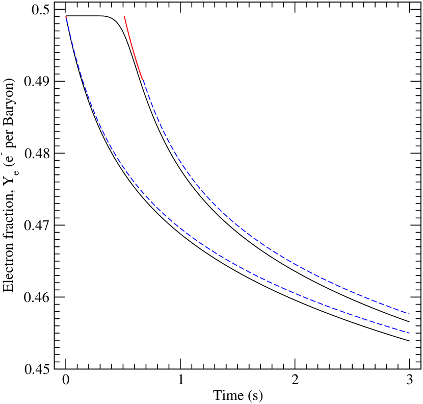
Figure 5.— The time history of $Y_{e}$ for two fluid elements burned by the artificial flame starting at a density of $10^{9}$ g cm^-3. The time history on the grid computed from the simplified burning model is shown in black, whereas the history computed in post processing is shown in red (reconstructed portion) and blue (direct post-processed portion). Two fluid elements are treated, one that begins the simulation in the burned state (lower black), and one that the flame passes through after 0.5 s (upper black).

In order to verify that the neutronization is captured well by this method, we turn to 1D simulations in a spatially uniform density medium. For a low Mach number flame in these conditions, a constant-pressure self-heating calculation is a good approximation to the correct fluid history (Vladimirova et al., 2006; Calder et al., 2007; Chamulak et al., 2007). A comparison of the $Y_{e}$ history obtained from the hydrodynamics and the fluid element history post-processed as described above is shown in Figure 5. The histories of two fluid elements are taken from a simulation in which an artificial flame is propagated from a hard wall into 50:50 CO fuel at a uniform density of $10^{9}$ g cm^-3 with a flame speed of $5\times 10^{6}$ cm s^-1. The first fluid element begins in the burned region. Its initial state is determined by the Rankine-Hugoniot jump conditions satisfied across the flame front as used to set the initial condition of the simulation. The second fluid element is taken from a position that the flame passes at about 0.5 s. The reconstructed portion of the post-processing is shown in Figure 5 by the solid red portion of the curves and the direct density-temperature history post-processed portion is shown by the blue dashed lines. The black curves show the $Y_{e}$ according to the burning model, Equation (20), at the fluid element position in the hydrodynamic simulation. The agreement is fairly good, with the change in $Y_{e}$ from 0.5 matching within a few percent for both the initially burned case and the case passing through the reconstructed portion at 3 s, a few times longer than expected exposure in an explosion simulation. This provides confirmation that scaling $\dot{Y}_{e}$ with $\phi_{qn}$ in the burning model provides a reasonable behavior even with a thickened reaction front. The difference between the $Y_{e}$ time history given by the simulation and the post-processing appears consistent with the use of a larger nuclide set to compute the neutronization rate tables used in the burning model (Seitenzahl et al., 2009b). Using a larger nuclear network for post-processing would improve this difference at some cost to efficiency.

Ideally the $Y_{e}$ histories of the two fluid elements would just be shifted by a time delay based on when their burning began. However, the flame propagation in physical space is slowing somewhat due to the loss of pressure due to neutronization of the earlier burned material. This causes the later burned fluid element to be at a slightly higher density at a given time interval after burning began. The first several tenths of a second of evolution match well in both cases, demonstrating that the post-flame state is consistent with the Rankine-Hugoniot calculation as expected.

4. Detonation Hydrodynamics

In this section we demonstrate the detonation structure we wish to reproduce and we test the burning model in hydrodynamic simulations in comparison to this benchmark. Although it was developed initially for deflagrations in carbon-oxygen mixtures, the reaction structure of detonations is similar enough (Khokhlov, 1983, 1989) that the 3-stage model can also be applied to them. In the simplest form, this just involves identifying the first stage, ¹²C consumption, with the rate of the actual ${}^{12}{\rm C}+^{12}{\rm C}$ reaction, and then following the later burning stages. This was done, for example, in Meakin et al. (2009), and we will do something similar here, with some adjustments for improved accuracy.

As can be inferred from the length scales shown in Figure 1, the actual burning structure is not resolved in full-star simulations. Therefore, somewhat like in the case of the deflagration, the dynamics which lead to the reaction front propagation are not the same in the simulation as in reality. The physics is similar; the energy release determines the strength, and therefore speed, of the detonation shock. However, the acoustic structure in the simulation is not the same as the physical detonation structure. Reactions must be suppressed in the numerically unresolved shock in order to prevent numerical diffusion from dominating the propagation of the reaction front (Fryxell et al., 1989). This creates an artificial separation of a few zones between the shock and the reaction zone. In addition, the reactions may run to near completion within the single zone in which reactions are re-enabled downstream of the shock. We show in Appendix A that the widely-used technique of disabling reactions in the zones adjacent to the shock reproduces the steady state detonation speed and the resolved portions of the reaction structure.

Here we present the error-controlled calculation of the 1D structure of planar detonations that we will use as our benchmark for both the burning model in hydrodynamics and the Lagrangian post-processing. After introducing this benchmark, the remainder of this section will focus on how, in comparison, the burning model acts in hydrodynamic simulations. Post-processing will be discussed in section 5. As already mentioned in the presentation of the burning model in section 2, simply treating $\phi_{fa}$ according to the C reaction rate and then proceeding as discussed in Townsley et al. (2007) turned out in testing to not reproduce partially-resolved detonation temperature and abundance structures at intermediate densities, $10^{6}$-$10^{7}$ g cm^-3. The successful comparison to benchmarks shown in this section is the result of making the required adjustments to the burning model timescales discussed in section 4.2.

4.1. Verification Benchmark: The ZND structure

In order to evaluate the realism of our simplified model of burning, it is necessary to define an authoritative reference with which it will be compared. Since, as one might expect, no direct experimental validation of nuclear detonations in stellar matter are available, we instead turn to a hierarchical approach to validation (Calder et al., 2002). Following this practice, our interest is in verifying that burning characteristics of our models are similar enough to those computed with methods in which we have more confidence. A typical benchmark in a hierarchical verification like this would be a direct numerical simulation (DNS) of similar phenomenon with more detailed, and typically separately verified, treatments of physical processes. Another source of benchmarks is particular configurations or steady states that can be computed more easily, for example in lower dimension, or in more detail and with better numerical error control.

As one of the two combustion modes in SN Ia explosions, the predicted outcome of C-O detonations have been discussed in some detail previously in the astrophysical literature. Khokhlov (1989) presented an overview of the microscopic structure of steady-state planar C-O and He detonations at a variety of densities. Further work by Sharpe (1999) extended calculations of the structure of the planar steady-state structure and products beyond the sonic point in the detonation wave, allowing the completion of burning to be computed at a wider range of densities. Sharpe (2001) followed this up with computations of detonation speeds and structure for non-planar, i.e. curved, detonation fronts in steady state, still in one dimension. Gamezo et al. (1999) and Timmes et al. (2000) investigated the multi-D structure of C-fueled detonations with high resolution reactive hydrodynamics for cases important for SNe Ia. Recently, Domínguez & Khokhlov (2011) performed a high-resolution investigation into the stability of C-fueled detonations in 1 spatial dimension at low densities, $\lesssim 10^{6}$ g cm^-3.

We are interested here in an inherently transient phenomena as the detonation traverses different densities within the star. As a result, the ideal benchmark is simulations of the reactive Euler equations which include all relevant nuclides (and therefore all relevant reactions) and in which all important length scales are resolved. The component models of such a DNS have been separately validated in many contexts, and their limitations are fairly well understood. Unfortunately, a DNS is challenging for the nuclear processes under consideration here. In order to fully capture the reaction kinetics, it is necessary to include hundreds of species. The more severe limitation, however, as demonstrated in Figure 1, is the large separation of time and length scales between the final reaction stages – those which process Si-group to Fe-group elements or perform electron captures – and the reactions which drive the burning front forward, fusion of carbon. At the densities of most interest, where the nucleosynthetic processing to Fe-group is incomplete due to the finite size of the star, a few $\times 10^{6}$ g cm^-3, these length scales are $10^{9}$ cm and $0.1$ cm respectively.

In this work, we will compare our results with those obtained from the well-known Zel’dovich, von Neumann and During (ZND) model of detonations (Zel’dovich, 1940; von Neumann, 1942, 1963; Döring, 1943; Fickett & Davis, 1979). This model predicts both the detonation velocities and final products as well as the detailed 1D thermal and compositional structure in space for steady state denotations. It can also be computed with error-controlled methods with a large reaction network including all relevant reactions. Matching these detailed structures during burning is crucial for our application. The ${}^{56}{\rm Ni}$ yield of the supernova will be determined by the burning processes that lead to these structures. Therefore, if our burning model, including particle post processing steps, can accurately reproduce the abundance profiles predicted by the ZND model, it increases our confidence in the yields that it predicts in more general cases.

The ZND equations describe the detonation structure between the detonation shock front and the sonic point. Beyond the sonic point, where the following flow is moving away from the detonation front at the local sound speed, disturbances cannot move upstream to change the detonation flow. The portion of a propagating steady-state detonation between the shock and the sonic point is a static (i.e. time invariant) structure which propagates in space at the detonation speed. The flow beyond the sonic point is typically not static, and its form depends on the boundary condition of the following flow. Sharpe (1999) computes the flow beyond the sonic point for asymptotically free propagation, but we do not undertake that here.

Before moving further in the discussion, it is useful to state the ZND equations in the form in which we will use them, for plane-parallel, steady-state detonations (Fickett & Davis, 1979; Khokhlov, 1989). In the frame of the detonation front,

$$v = \frac{\rho_{0}D}{\rho}\ ,$$ (41)

$$\dot{\rho} = \frac{\Sigma}{v^{2}-c_{s}^{2}}\ ,$$ (42)

$$\dot{T} = \left(\frac{\partial T}{\partial P}\right)_{\rho,Y_{i}}\Bigg{\{}\left[v^{2}-\left(\frac{\partial P}{\partial\rho}\right)_{T,Y_{i}}\right]\dot{\rho}$$ (43)

$$\quad\quad\quad\quad\quad\quad\quad\mbox{}-\sum_{j}\left(\frac{\partial P}{\partial Y_{j}}\right)_{\rho,T,Y_{i\neq j}}\dot{Y}_{j}\Bigg{\}}\ .$$

Here dot indicates an ordinary time derivative, $d/dt$, $v$ is the flow velocity (with respect to the detonation front), $\rho_{0}$ is the unburned density, $D$ is the detonation speed, $c_{s}$ is the frozen (evaluated with constant $Y_{i}$) adiabatic sound speed, $P(\rho,T,Y_{i})$ is the pressure. To be consistent with the above conventions, $Y_{i}$ is the number of nuclei of nuclide $i$ per fluid baryon. Thus $Y_{i}=X_{i}/A_{i}$, where $A_{i}$ is the mass number of nuclide $i$. The $\dot{Y}_{i}$ are given by the nuclear reactions. The energy release function, in the absence of weak interactions, is

$$\Sigma=\left(\frac{\partial P}{\partial\mathcal{E}}\right)_{\rho,Y_{i}}\left[\sum_{i}B_{i}\dot{Y}_{i}-\sum_{j}\left(\frac{\partial\mathcal{E}}{\partial Y_{j}}\right)_{P,\rho,Y_{i\neq j}}\dot{Y}_{j}\right]\ ,$$ (44)

where $\mathcal{E}$ is the internal energy. The integration of these equations is begun just behind the leading shock, whose properties are related to those of the fresh fuel by the detonation speed $D$ and the usual shock conservation equations.

A diagram of the form of typical solutions are shown in Figure 6. Equation (42) is singular at the sonic point, where $v=c_{s}$, unless $\Sigma$ is also zero there. There is a large class of solutions for which $D$ is high enough that the entire following flow is subsonic. That is, $\Sigma$, and therefore $\dot{\rho}$, changes sign from negative to positive before $v$ increases to $c_{s}$, thus avoiding an encounter with this singularity. This type of solution has a higher pressure in the final state than in the reaction zone, and is called ”overdriven” or ”supported” since it is effectively being pushed from behind by an overpressure. In this case the full flow, including $D$ itself, has an inherent dependence on this boundary condition. As the pressure in the final state, or at the ”piston” following the detonation, is decreased, $D$ also drops, and eventually a sonic point will appear. For detonations with lower pressures in the following flow, the steady portion of the detonation flow then becomes an eigenvalue problem such that $\Sigma=0$ at the sonic point.

In simplified reaction systems, $\Sigma=0$ at the sonic point because that is the point at which fuel consumption completes. This is called a Chapman-Jouget detonation (Fickett & Davis, 1979), and its speed can be computed from just the energy release and the EOS, without a need for the full ZND equations (Khokhlov, 1989; Gamezo et al., 1999). For reaction systems with complex or reversible reactions or changes in mean molecular weight, the heat release function $\Sigma$ may not reach or cross zero at a unique level of progress toward the fully burned state. That is, $\Sigma=0$ may be attained before burning is ”complete” and a static final state reached. In this case, the sonic point, and thus the end of the static portion of the detonation profile, also occurs before a stable final state is reached. Such a detonation is termed ”pathological” or ”eigenvalue” and the sonic point, where the singularity appears in the ZND equations, and where, therefore $\Sigma=0$, is called the pathological point. This is, in fact, the more common case, and eigenvalue detonation structures in this case represented a major advancement manifest by the ZND model (Fickett & Davis, 1979).

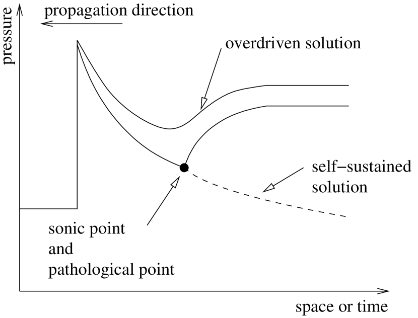
Figure 6.— Detonation pressure structure in space and time for a steady-state detonation in 1 dimension. The lower solid and dashed lines that pass through the pathological point represent possible solutions for the cases in which the sonic point is reached before completion of burning. These detonations are termed ”pathological” or ”eigenvalue” detonations.

The ZND integration can be continued after passing through the pathological point, but there is more than one way to exit this point (Sharpe, 1999). Figure 6 shows a diagrammatic representation of the relation of the pressure profile in overdriven and self-sustained, or unsupported, detonation. The lowest overdriven detonation which can be fully integrated using just the ZND equations without traversing a singularity is that which passes just above the pathological point. While it is possible with special methods to traverse the pathological point and obtain the self-sustained solution (Sharpe, 1999; Moore et al., 2013), we do not undertake this here due to our large set of species and complex reactions. This seems prudent because even some of the profiles obtained by Sharpe (1999) using this method show clear indications of having further zero-crossings of $\Sigma$ beyond the pathological point. How these would manifest in the detonation structure is unclear from this level of analysis.

It is now possible to choose a well-defined verification benchmark problem whose solution can be calculated with both the ZND model with a fairly complete reaction set and a 1D hydrodynamic simulation with our simplified burning model. We choose our benchmark to be the slightly-overdriven state found by tuning $D$ to be a small amount above the eigenvalue that leads to the pathological point. This configuration can be replicated in a 1D hydrodynamic calculation by manipulation of the boundary conditions in the following flow to have the appropriate pressure in the fully burned state. The static portion of the benchmark structure, between the shock and the sonic point, can be also used as a reference solution for self-sustained detonations once they reach steady-state.

4.2. Calibration of Timescale for Si Consumption

In order to make use of the simplified dynamics for the transition from the QSE to the NSE state, given by Equation (27), we must calibrate the timescale $\tau_{\rm NSE}$. In Calder et al. (2007), $\tau_{\rm NSE}$ was calibrated by computing the consumption timescale in isochoric self-heating as a function of temperature and then using a fit to that timescale for $\tau_{\rm NSE}$. Here we will compare the time evolution of Si group element abundances for our benchmark detonation, computed using the ZND equations, directly to the behavior posited in our burning model by Equation (27).

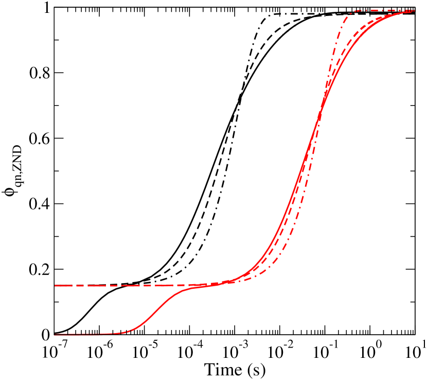
Figure 7.— Effective progress variable for the conversion of Si- to Fe-group material, or relaxation toward full NSE (see text for definition). Driven detonations computed by a ZND integration are shown at two pre-shock densities of $10^{7}$ g cm^-3 (black, shorter timescale), and $0.5\times 10^{7}$ g cm^-3 (red, longer timescale). Also shown are fits to the dynamics in the current burning model (dashed lines) and exponential relaxation (dot-dashed lines).

In order to make comparisons we use $\phi_{qn,\rm ZND}\equiv\phi_{qn}(X_{i})$ based on Equation (38), where the $X_{i}$ are the abundances from the ZND calculation computed with a large network for a driven solution. In Figure 7, $\phi_{qn,\rm ZND}$ is shown for two densities spanning the range of interest, 0.5 and $1\times 10^{7}$ g cm^-3. From Figure 1 we see that at these densities the synthesis of IGE from IME will occur as a partially or mostly resolved process on the grid during the explosion of the star, and will largely determine the IGE yield of the explosion. Expansion times for the star are in the range of a few tenths of a second and the hydrodynamic timestep is around $10^{-4}$ s for typical simulation resolutions of a few km.

As will be shown in section 4.3, the early rise to $\phi_{qn,\rm ZND}\approx 0.15$ in both curves is due to IGE+LE produced during the oxygen consumption stage. Therefore we will proceed by fitting the latter part of the curve only to get a better characterization of the transition timescale. If necessary, the inclusion of some IGE in the intermediate state, $\xi_{q,i}$ in Figure 3, could be introduced in converting the progress variables to abundances. However since we use post-processed yields for our final abundances this is not necessary.

In the C-O burning process, the stages are well enough separated in time that oxygen consumption, which is complete about the same time the Si abundance peaks, completes before the transition from Si- to Fe-group proceeds very far. This can be seen clearly in Figure 1 as the 5 orders of magnitude separating the time of maximum Si abundance (dashed red line) and the completion of burning (solid red line). We therefore assume $\phi_{aq}=1$ and for a characteristic value of $\tau_{\rm NSE}$ we may analytically integrate Equation (27) to obtain

$$\phi_{qn}(t)=\phi_{qn,\rm final}-\frac{1}{1/(\phi_{qn,\rm final}-\phi_{qn,0})+t/\tau_{\rm NSE}}\ .$$ (45)

Here $\phi_{qn,0}$ and $\phi_{qn,\rm final}$ are taken from $\phi_{qn,\rm ZND}$ at the end of oxygen consumption and in the final state respectively. In this case they are about 0.15 and 0.99. $\phi_{qn,0}$ might be different if we performed this calibration with different initial abundances. This form can now be fit to the curves shown in Figure 7 using a non-linear least squares fit. We use a fitting region $0.15\leq\phi_{qn}\leq 0.85$, to capture the major portion of the evolution. The resulting fits are shown by the dashed lines. The fit timescale is not sensitive to choice of $\phi_{qn,0}$; a 5% variation in $\phi_{qn,0}$ only changes the fit $\tau_{\rm NSE}$ by 1%. The maximum error in the fits occurs when $\phi_{qn}\approx 0.4$, and is about 0.06 and 0.03 for the higher and lower density shown in Figure 7 respectively. We will discuss below in section 4.3 how well the resulting burning model performance in hydrodynamics compares to the detonation benchmark, and extend this comparison to abundances in post-processing, compared to those in the benchmark, in section 5.

This fitting procedure has been repeated at several densities, between 0.3 and 10 $\times 10^{7}$ g cm^-3. At each of these densities the conversion of Si- to Fe-group takes place at a declining temperature. The decline during this burning stage is, however, much less than the variation from one density to another. By evaluating the temperature when the relaxation is approximately half complete, we can construct and fit a relation between $\tau_{\rm NSE}$ and $T$. We obtain

$$\tau_{\rm NSE}(T)=\exp(201.0/T_{9}-46.77)\ .$$ (46)

The $\tau_{\rm NSE}$ timescale found here is not directly comparable to previous work because we have used different burning dynamics. However, a similar fit can be performed with the exponential decay form that results from the simpler dynamics previously posited, $D\phi_{qn}/Dt=(\phi_{aq}-\phi_{qn})/\tau_{\rm NSE}$ (Townsley et al., 2007). This is shown by the dot-dashed lines in Figure 7 when fit to the same region indicated above. This form does not appear to provide a good reproduction of the late-time behavior of $\phi_{qn}$. Also the timescales obtained for the exponential fit are approximately a factor of 10 to 20 shorter than those given for $\tau_{\rm NSE}$ in Calder et al. (2007). This is understandable because the definition used in that work measured a timescale to reach a fairly complete burning stage, whereas we have fit an exponential form directly.

4.3. Comparison of parameterized burning hydrodynamics against 200-nuclide ZND Structure

The verification that we are attempting to perform involves demonstrating that the abundance structure produced by post-processing particle tracks from the hydrodynamics which utilizes the parameterized burning matches the ZND structure for a steady state detonation. That comparison will be done in section 5, but first it is useful to compare the intermediate result obtained from the parameterized burning model in the hydrodynamics simulation alone. This will provide a check on the realism of spatial thermodynamic structure without the added complication of the integration of the Lagrangian tracks, and also give some diagnostics concerning whether the parameters within the burning model are behaving as expected.

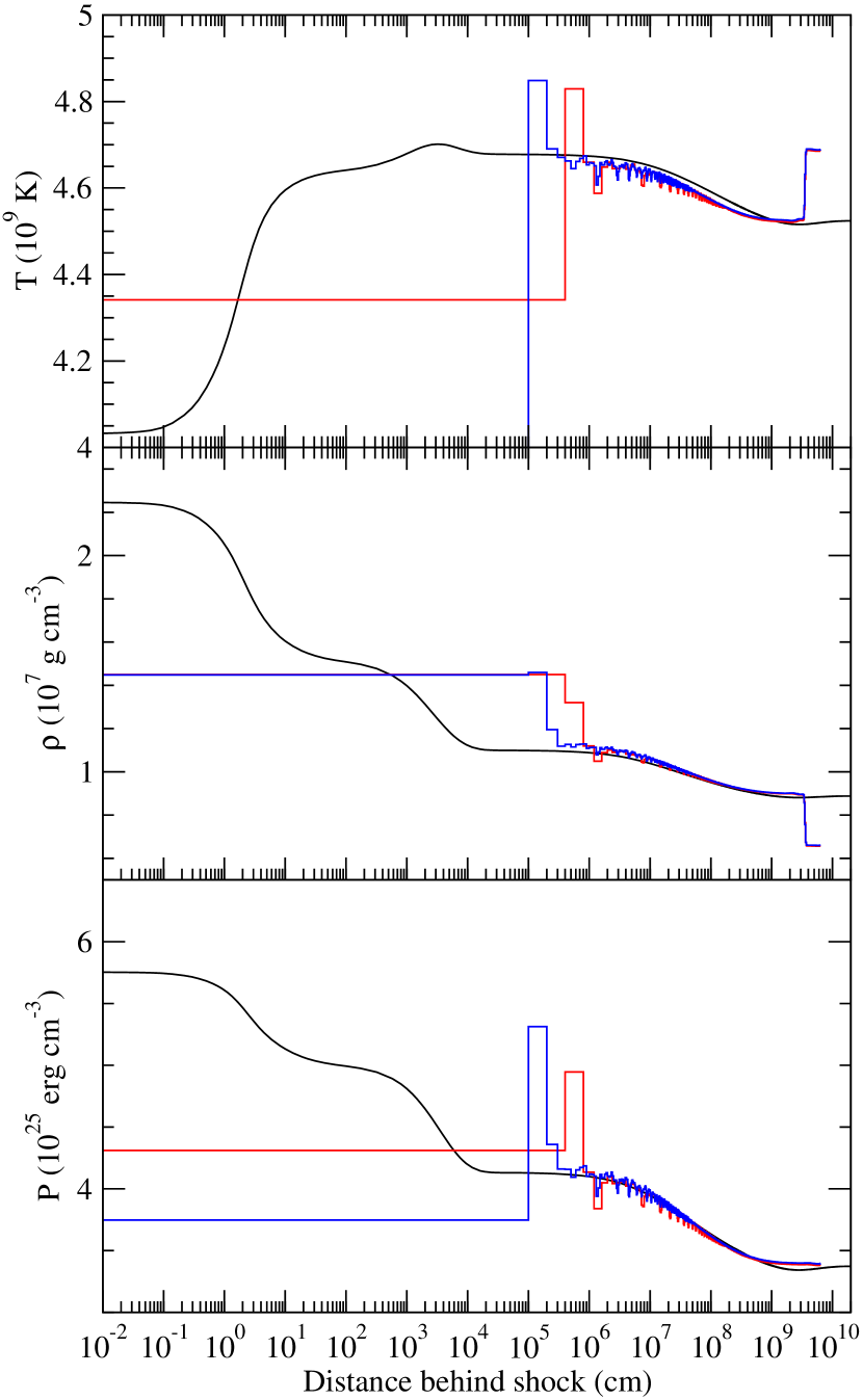
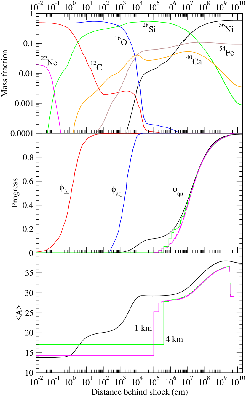
Figure 8.— Detonation thermal and composition structure displayed by our parameterized model for C-O burning in 1D hydrodynamic simulations compared to our detonation benchmark of the steady-state ZND solution of the equivalent detonation. This case is at a density of $\rho=5\times 10^{6}$ g cm^-3 and an initial composition of 50% ¹²C, 48% ¹⁶O and 2% ²²Ne. Left: Thermal structure of simulations at spatial resolutions of 4 km (red) and 1 km (blue) compared to the benchmark steady-state ZND solution (black). Right: Top: The composition structure of the benchmark ZND calculation computed with a 200-nuclide network. Middle: Effective progress variables derived from the abundances in the benchmark (red, Equation (47); blue, Equation (48); black, Equation (38)), compared to the $\phi_{qn}$ progress variable obtained in the hydrodynamic simulations at 4 km (green) and 1 km (magenta) resolution. Bottom: Average number of nucleons per nucleus, $\bar{A}=1/Y_{\rm ion}$, derived from the full abundances in the benchmark (black) and obtained from the progress variables, Equation (21), in 1D hydrodynamic simulations at 4 km (green) and 1 km (magenta).

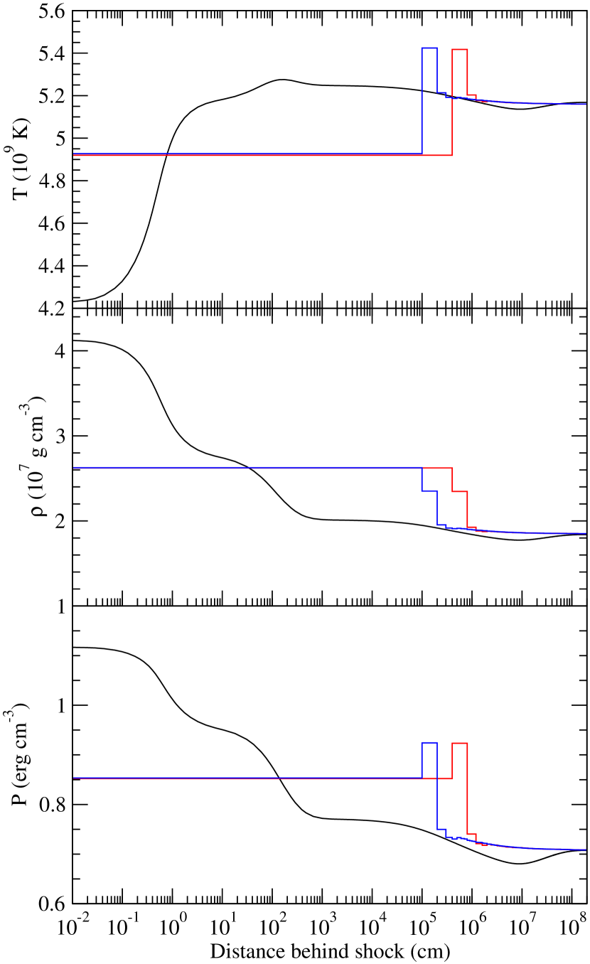
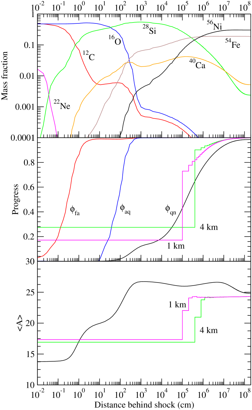
Figure 9.— Similar to Figure 8 but for $\rho=10^{7}$ g cm^-3.

Our benchmark is, as described in section 4.1, the ZND solution for a steady-state, planar, slightly overdriven detonation in 1 dimension. This solution is shown as the reference curves in Figures 8 and 9, with thermodynamic quantities, $T$, $\rho$, $P$, in the left panel (black), and abundances in the top right panel. The initial condition for the 1D hydrodynamic simulations is material at spatially constant density and temperature away from the ignition point. We consider cases here with this background temperature set to $4\times 10^{8}$ K. The domain extends from $x=0$ to $65,536$ km in order to allow the detonation to approach steady state. Two resolutions, 4 km and 1 km, similar to the resolution of production supernova simulations (Townsley et al., 2009), are used to confirm insensitivity to resolution. We will refrain from using the term convergence here, reserving it for circumstances in which gradients are resolved. The boundary condition on the opposite end of the domain from the ignition is reflecting, but has no impact on the simulation due to the supersonic nature of the detonation and since the simulation is stopped before the front reaches it. The left boundary, at $x=0$, is a zero-gradient boundary. The initial perturbation is made in both temperature and velocity. Along with inflow from the zero-gradient boundary, the latter will serve to support the detonation from behind. Both temperature and velocity are placed as linear gradients decreasing from a maximum at $x=0$ to the background values of $T=4\times 10^{8}$ K and velocity of zero over a size we will call the size of the ignition region. The velocity is tuned by hand until the pressure far behind the detonation front and near the $x=0$ boundary matches the late-time pressure found for the slightly overdriven ZND solution. Ignition region sizes were 1024 km and 128 km for $10^{7}$ and $5\times 10^{6}$ g cm^-3 respectively.

As above, we will focus on densities at which the transition from Si-group burning products to Fe-group burning products is fully or partially resolved on the spatial grid. At a density of $5\times 10^{6}$ g cm^-3, as indicated by Figure 1, nearly the entire Si- to Fe-group transition is resolved at 4 km resolution for the steady state detonation. The spatial structure obtained from the ZND calculation and the hydrodynamics, which uses the parameterized burning, is shown in Figure 8. The thermodynamic quantities, $T$, $\rho$, and $P$, are shown in the left panel. The hydrodynamic result is at an evolution time of 5.45 seconds, when nearly the entire domain has been consumed. The zero point for the distance behind the shock in the hydrodynamic simulations is taken as the last zone in which the shock detection considers the cell inside a shock, thereby suppressing the reactions in that zone. See Appendix A for more on this suppression. In steady state, the shock region in which the reactions are suppressed is a well-localized region of approximately 4-5 zones. As a result of this, the first point from the hydrodynamic simulations, indicated with stair-stepped lines, is at 4 km and 1 km for simulations of those respective resolutions. The top right panel shows the spatial abundance structure of a selection of nuclides for the steady-state detonation from the 200-nuclide ZND calculation. From the ZND abundance and thermal structures shown in Figure 8 we see that both the ¹²C and ¹⁶O consumption stages are entirely unresolved because they take place on length scales of approximately 1 cm and several $\times 10^{3}$ cm respectively. In the span of less than a single zone, the burning reaches the Si-rich QSE.

The values of $P$, $T$, and $\rho$ at the point chosen as zero distance behind the shock in the simulation are not quite the same as the post-shock values expected based on the detonation speed. This is presumably the result of numerical mixing in the vicinity of the under-resolved shock and burning front. The post-shock density is about 35% lower than the peak value predicted by the ZND calculation and the pressure, rather than peaking at the shock, peaks in the first zone in which burning is allowed at a value about 10% lower than expected. The $T$ peak, which also occurs in the first zone in which reactions are allowed, is about 3% higher than the peak in the benchmark. This transient is also larger in time and space than the true burning structure due to the resolution, but the thermal state appears to relax back toward a good approximation of the QSE state very quickly, within 2 zones. After this and a small undershoot, the hydrodynamic solution is a very good match, with 3% in $P$ and $\rho$, and within about 1% in $T$, all the way out to the pathological point. There is noise on a similar level, but more so in $P$ and $T$ than $\rho$. An artifact of the initial ignition is evident at the end of the hydrodynamic curves for $T$ and $\rho$. We also find very good consistency between resolutions after the first few zones behind the shock, matching within a percent, with noise in each case slightly larger than that. The hydrodynamic result is probably not completely relaxed to the steady-state overdriven solution, since there is no pressure minimum. However, the pathological point occurs quite close to the end of the domain even for this large domain and the pressure minimum is expected to be fairly shallow.

A comparison of some of the parameters in the burning model are shown in the lower right two panels in Figure 8. In order to make a comparison of the progress variables we have defined some effective progress variables for the 200-nuclide set. In addition to Equation (38) above, we define

$$\phi_{fa}(X_{i}) = 1-\frac{X_{{}^{12}\rm C}}{X_{{}^{12}\rm C,0}}\ ,$$ (47)

$$\phi_{aq}(X_{i}) = 1-\frac{X_{{}^{18}\rm O}}{X_{{}^{18}\rm O,0}}\ .$$ (48)

The spatial structure of both $\phi_{fa}$ and $\phi_{aq}$ are unresolved at this density and these resolutions. Thus they are both 1 in the first zone behind the shock-detection suppression of burning because our data dumps always follow a reaction sub-step in our operator split time evolution. For this reason the $\phi_{fa}$ and $\phi_{aq}$ from the hydrodynamic simulations are not shown.

We find a good match between the evolution of $\phi_{qn}$ and the effective equivalent defined for the 200-nuclide set. The largest discrepancy is due to the production of some Fe-group material with Si-group in the benchmark. After $\phi_{qn}\gtrsim 0.3$ the discrepancy is less than $0.05$, and after $\phi_{qn}\gtrsim 0.5$ it is less than $0.02$. This indicates that our temperature-dependent fits of the timescales for this evolution, described in section 4.2, are acting satisfactorily. The bottom right panel of Figure 8 shows how the mean ion molecular weight $\bar{A}$ compares to the equivalent quantity from the parameterized burning $1/Y_{\rm ion}$. This quantity is systematically about 4% low, probably due to our choice of $\tilde{Y}_{\rm ion,QSE}=1/28$ as an estimate of the $Y_{\rm ion}$ of the QSE state. The QSE state is not pure ²⁸Si, and therefore this estimate is slightly off and creates a systematic offset in the consecutive evolution toward $Y_{\rm ion,nse}$. The difference observed in the test may also be magnified by the hydrodynamic simulation having not quite reached the steady overdriven state. In either case the discrepancy in $\bar{A}$ only leads to less than 1% discrepancy in $T$, as found above, so this level of agreement appears sufficient for producing accurate thermodynamic histories for particle post-processing.

As a second case, shown in Figure 9, we perform a similar calculation at an ambient density of $10^{7}$ g cm^-3. At this density, more than half of the transition from the Si-group dominated QSE to the Fe-group dominated NSE is unresolved on a 4 km grid. This is according to the profile of $\phi_{qn}$ predicted by the 200-nuclide ZND calculation, shown in the middle right panel of Figure 9. We see a region, similar to that in the first case, of about 2 zones in which $T$ is about 3% higher than the expected peak and $P$ and $\rho$ are intermediate between the expected post-shock values and the QSE values, after which all of these relax to within 3% of the benchmark values. The largest source of discrepancy is due to the lack of the expected minimum near the pathological point at a distance of $10^{7}$ cm behind the shock. Instead, the hydrodynamic solution monotonically relaxes to the state given by the boundary condition pressure. However, even with this discrepancy the maximum difference between the benchmark and hydrodynamic result is about 5% in $P$ and $\rho$ and less than 2% in $T$. As before the two resolutions match very well, within 0.5%.

In terms of progress variables, during the partially-resolved transition from Si- to Fe-group, the progress variable for this process, $\phi_{qn}$, is about 0.1 higher than the benchmark predicts at a given distance behind the shock. This seems like a reasonable indication of the uncertainty of the progress variable’s reproduction of the real process for partially-resolved cases like this one. The $\bar{A}$ determined in the final state by the burning model in the hydrodynamics is only about 2% lower than the benchmark. However, as for the thermal profiles, the non-monotonic behavior near the pathological point is not captured.

The main difference from the benchmark in this case is due to the lack of a clear pathological point in the hydrodynamic result. It is unclear if this is due to the limited resolution, a deficiency in the burning model, or insufficient time to relax to the steady state. In any case, the discrepancy in the thermal quantities used for post processing is, at maximum, a fairly modest 5% in $\rho$ and 2% in $T$. We will accept this as the approximate uncertainty in the thermal histories produced by the burning model, and proceed to investigate the abundances produced in post-processing directly below. At higher densities than about $10^{7}$ g cm^-3, as can be seen from the length scale for completion of Si- to Fe-group conversion, the conversion will be nearly complete on scales smaller than the resolution. The burning model shows good reproduction of the final state, within a few percent, so that denser cases should also have similar good accuracy.

5. Verification of Lagrangian particle nucleosynthesis against ZND solution

While it is important that the progress variables provide a good reproduction of the detonation structure, in the end the yields will be computed by post-processing Lagrangian tracer particle histories. In this section we compare computed Lagrangian track yields to the steady-state ZND solutions that we are using as a benchmark. Detonation yields are computed by a direct integration of the $\rho(t)$, $T(t)$ history recorded by the Lagrangian tracer particle from the hydrodynamic simulation, using them to set the reaction rates in the nuclear reaction network.

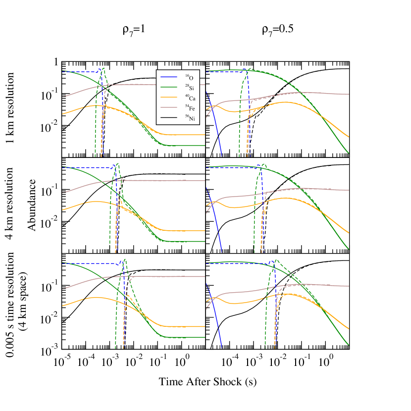
Figure 10.— Abundance histories computed from post-processed Lagrangian histories from hydrodynamic simulations (dashed lines) compared to benchmark steady-state detonation structures computed from the ZND equations (solid lines). Shown as mass fractions are the major abundances after C consumption, ¹⁶O (blue), ²⁸Si (green), and ⁵⁶Ni (black), as well as ⁴⁰Ca (orange) and ⁵⁴Fe (brown). Two densities are shown, $10^{7}$ g cm ^-3 (left column) and $5\times 10^{6}$ g cm^-3 (right column). Each of these is shown from a simulation with 1 km (top row) and 4 km (middle row) spatial resolutions with histories recorded at full time resolution, and at 4 km spatial resolution with history recorded at a reduced time resolution of $0.005$ s (bottom row).

The results of the integration of the reactions over the Lagrangian history are compared with benchmark calculations in Figure 10 for the same two densities, $10^{7}$ and $5\times 10^{6}$ g cm^-3 (left and right columns), and two spatial resolutions, 1 km and 4 km (top and middle row), as used in Section 4.3. We also consider a case with a reduced time resolution for the recording of the Lagrangian history (bottom row). Comparison can now be made directly with actual abundances. We show the major abundances for stages beginning at oxygen consumption, ¹⁶O, ²⁸Si, and ⁵⁶Ni, as well as the major neutron-rich nuclide produced before other Fe-group material, ⁵⁴Fe (Bravo et al., 2010), and the spectroscopically important ⁴⁰Ca. Each plot shows two curves for each nuclide: the benchmark solution (solid lines) computed using the ZND equations and the post-processing of the $\rho(t)$, $T(t)$ history (dashed lines).

In order to compare structures we must choose a zero time during the Lagrangian history. Zero time for the benchmark ZND integration corresponds to the downstream side of the shock. We have chosen the zero time for the Lagrangian history to be at the first timestep that reaches 1% above the ambient temperature. This makes the entire reaction region visible on these plots because the C and O consumption timescales in the benchmark are shorter than the timestep in all cases. The abundances in the first part of the reaction region are unrealistic, as expected. Notably at $\rho_{7}=1$ the ²⁸Si abundance during the first few steps overshoots what should be present. However, the abundances appear to recover quickly to fairly accurate values within 0.01 s in all cases with full time resolution in the history. For the coarsened time resolution history shown in the bottom row, the recovery toward the correct solution is slower, taking until nearly 0.1 s at $\rho_{7}=0.5$. This is comparable to the expansion timescale of this material during the supernova and indicates that a time history at the same time resolution as the hydrodynamics is required at this density.

In comparison to the benchmark solution we find excellent agreement after 0.01 s. The worst case is ²⁸Si at $\rho_{7}=1$, 4 km resolution, off by less than 0.005, about 20% of the abundance at that time. More typical discrepancies are those near where ⁵⁶Ni and ²⁸Si are similar abundance for $\rho_{7}=0.5$, which are between 5 and 10%. This comparison verifies directly, for the first time in the computation of thermonuclear supernovae, that a hydrodynamic calculation with post processing correctly reproduces detonation yields computed with an error-controlled integration of the ZND model. Thus the dynamics in our parameterized burning model is able to give sufficiently accurate thermodynamic structures for post-processing abundance calculations accurate to between 5 and 10% for steady-state planar detonations down to $\rho_{7}=0.5$. This includes densities at which the detonation structure is partially resolved. The driving region extends to near the plateau of the ⁵⁶Ni abundance, as can be inferred from the location of the density and temperature minima near the pathological point in the ZND integrations shown in Figures 8 and 9.

6. Computation of Complete Nucleosynthesis

The previous sections have outlined methods for treating fluid elements within the star processed by either the detonation or deflagration modes of burning. In order to obtain yields for an actual computation of a DDT SNIa, it is necessary to perform both of these methods on the fluid element histories of a single simulation. This involves sorting and classifying histories to be treated with the two different methods and treating cases that may overlap. Also some aspects of the implementation of energy release in the hydrodynamics must be modified to allow both types of reactions. Here we discuss these and other details of the unified post-processing.

6.1. Track Classification

We begin by discussing how a Lagrangian history recorded from the hydrodynamics, hereafter called a “track” is classified as being processed either in a deflagration or detonation. This determines how the first portion of the post-processing is performed, which may involve reconstruction and replacement of an unresolved portion of the time history.

The recorded values of $\phi_{\rm RD}(t)$ and $\phi_{\rm fa}(t)$ for a track are scanned starting from the beginning of the time history. In searching for a detonation, the first few points are ignored after which we search for a sudden increase in $\phi_{\rm fa}$ to near unity. This indicates a detonation. The actual parameters used are for $\phi_{\rm fa}>0.9$ and $\phi_{\rm fa}$ having increased by more than 0.2 since the 4th previously recorded $\phi_{\rm fa}$. If the track is determined to be a detonation, it is subject to a direct post-processing of its $\rho(t)$, $T(t)$ history.

During the search for a possible detonation feature, if $\phi_{\rm RD}$ exceeds 0.5 before a detonation is detected, the track is classified as a deflagration. For a deflagration, the post-processing begins from the point in the time history at which $\phi_{\rm RD}=0.5$ and proceeds initially with a reconstruction as discussed in section 3. This calculation is changed to a direct post-processing at the time any of 3 conditions are met: $\phi_{\rm fa}>0.95$, $P<10^{22}$ erg cm^-3, or $\phi_{\rm fa}-\phi_{\rm RD}>0.1$. The latter condition is in addition to those mentioned in section 3, and most likely indicates that a fluid element passing through the artificially thickened flame front has been struck by a detonation shock. These borderline cases are some of the most challenging for for obtaining accurate yields. Several such examples are discussed along with others in Appendix B.

A track which does not meet either of the above criteria for detonation or deflagration will be assumed to have not been processed by either the deflagration and detonation and will be post-processed directly based on the $T$, $\rho$ history recorded.

6.2. Mixed Burning Modes in Hydrodynamics

As implied above, a fluid element with $\phi_{\rm RD}<0.5$ will not be considered to have been burned by the deflagration for the purposes of post-processing. This also has implications for the hydrodynamic implementation of the energy release: a detonation must be able to propagate into regions where $0<\phi_{\rm RD}<0.5$, i.e. regions that have been partially burned by the RD front that is propagating the deflagration. This presents a challenge because the temperatures in these regions are not physical and therefore can’t be used directly to compute a reaction rate like the $\dot{\phi}_{\rm CC}$ appearing in Equation (25). In order to allow detonations to propagate fully into the artificially broad deflagration reaction front, this issue is treated directly in energy release in the hydrodynamics rather than in post-processing.

Typically $\dot{\phi}_{\rm CC}$ is suppressed when $\phi_{RD}$ is larger than some small threshold. In order to allow thermal burning in these regions without it getting out of control, two measures are taken. First, $\dot{\phi}_{\rm CC}$ is only re-enabled in the proximity of non-flame-related burning. Carbon reaction unrelated to the deflagration is taken to be present if $\phi_{\rm fa}-\phi_{\rm RD}>\delta_{b}$, where $\delta_{b}$ is a threshold calibrated based on trials. $\delta_{b}=0.1$ has been found to be suitable in 2D and $\delta_{b}=0.3$ in 3D. For a given cell in the Eulerian hydrodynamics, proximity of thermally activated burning is established if this condition is satisfied in neighboring cells within one width of the RD front away, typically 4 cells. This allows $\dot{\phi}_{\rm CC}$ to activate when a detonation arrives at the RD front.

The second control measure attempts to estimate the temperature of the fuel in the absence of the deflagration rather than use the local $T$ directly in the computation of $\dot{\phi}_{\rm CC}$. Recall that the zones in which $0<\phi_{\rm RD}<1$ should be thought of as being regions of mixed burned and unburned material separated by a thin surface which is the propagating physical flame, each in approximate pressure equilibrium with the other. We would like to estimate the temperature of the unburned material. This is done by removing the energy which corresponds to the current amount of material burned and then computing the $T$ that corresponds to the energy leftover at the local $\rho$. This is a very rough calculation, but is only meant to be an estimate. The resulting temperature is then used to calculation $\dot{\phi}_{\rm CC}$.

6.3. Initial Abundances

In order to perform post-processing with a large network, it is necessary to specify a full set of initial abundances. These initial abundances must reflect the previous processing of the material in the star by earlier phases of evolution including the burning phases of the progenitor star and the core convection that precedes the ignition of the deflagration. Our initial abundances are parameterized by three parameters: the ¹²C abundance at ignition, the metallicity of the progenitor, and the $Y_{e}$ of the material, parameterized in the hydrodynamics by the mass fraction of ²²Ne in the fuel. The value of each of these for a given track is determined based on location of the tracer particle within the progenitor WD at the beginning of the simulation. Note that $Y_{e}$ is not the same parameter as metallicity due to the additional electron captures that occur during the pre-explosion core convection phase.

Given these parameters, the initial abundances are constructed from 4 components: (1) ¹²C of the specified mass fraction. (2) Metallicity given by scaled solar abundances of all elements heavier than ⁴He (Anders & Grevesse, 1989) except with the abundances of C, N, and O added together to give the abundance of ²²Ne used for the initial abundances (Timmes et al., 2003). (3) Ashes from the convective phase made up of equal parts ²⁰Ne, ¹⁶O, ¹³C, and ²³Ne (Piro & Bildsten, 2008; Chamulak et al., 2008). (4) The remainder is taken to be ¹⁶O. The contribution associated with the metallicity is assumed to be uniform throughout the star and any additional depletion of $Y_{e}$ in the interior convection zone is matched with the necessary amount of simmering ashes.

7. Results: 2D DDT Yields

Our model of SNe Ia using 2D simulations with a DDT is intended to reproduce the large-scale abundance distribution observed in the ejecta of normal SNe Ia. The most accessible observational characterizations are the abundance tomography studies (Stehle et al., 2005; Mazzali et al., 2008), though these do require some information about the ejecta as input, and therefore are not free of assumptions. Reproduction of abundance structure inferred from spectra is one of the metrics by with the original W7 model (Nomoto et al., 1984) and the 1D DDT models (Höflich et al., 1995) are found to succeed. Here we will compare our yields to these tomographic reconstructions and the essential aspects of successful theoretical models.

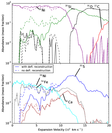
Figure 11.— Abundance profile of ejecta in velocity for 2D DDT simulation. Upper and lower panels show different species from the same simulations. Yields are averaged in spherical shell bins in velocity. Cases are shown in which the unresolved portion of the deflagration is explicitly reconstructed (solid lines) and in which the temperature-density histories are directly processed without reconstruction (dashed lines). The main impact of reconstruction is in capturing the peak temperature of the deflagration front, giving more complete burning of Si- to Fe-group in the interior.

Figure 11 shows the nucleosynthetic yields for major species from our 2D DDT simulation with ignition distribution realization number 10 from Krueger et al. (2012) using the progenitor from that work with a central density of $2\times 10^{-9}$ g cm^-3. The state shown is 4 seconds after ignition when the ejecta reaches approximate free expansion. The Lagrangian tracer particles from the simulation are binned based on their asymptotic radial velocity into bins of 250 km s^-1 width. For each bin, 100 randomly selected particles are post-processed as described in previous sections. See Appendix C for a discussion of the uncertainty arising from this choice of sampling. For the purpose of comparison, we perform nucleosynthetic post-processing both with and without the reconstruction of the portion of deflagration histories within the artificially broadened reaction front, as discussed in Section 3. Without this reconstruction, particle tracks are simply processed using their $\rho(t)$, $T(t)$ history.

The abundance content of the ejecta from our 2D DDT simulations compare fairly well with the general features seen in observations and the W7 profile (Stehle et al., 2005; Mazzali et al., 2008). Si group material is fairly well-separated from the inner layers of Fe-group that is dominated by ⁵⁶Ni. Reconstruction of deflagration tracks leads to more complete conversion of IME to IGE in the 2 000-10 000 km s^-1 region due to the higher peak temperatures reached using reconstruction. A notable difference from W7 is the absence, in our model, of a contiguous region near the center that is depleted in ⁵⁶Ni. This loss of such a core of stable Fe-group material was seen also in our earlier work (Krueger et al., 2012), and has since also been seen in 3D simulations as well (Seitenzahl et al., 2013). It appears that without recourse to other mechanisms of neutron enrichment in the core, the deflagration ash distribution produced by multi-D DDT simulations does not in general produce an unmixed core of stable Fe-group.

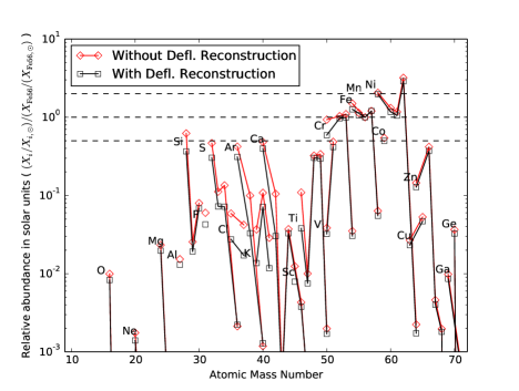
Figure 12.— Isotopic yields in units of solar abundances and scaled to the ⁵⁶Fe yield. Isotopes of a single element are connected by a line. Results of post processing particles with two methods are shown, in which the $rho$, $T$ history of the particle is used directly (without deflagration reconstruction, red diamonds), and one in which the portion of the history within the artificial reaction front is reconstructed (with deflagration reconstruction, black squares). Dashed boundary lines at 0.5 and 2 are also shown for reference. Differences in the Fe group are mild, but the relative yield of IME is lower.

The isotopic distribution in the overall yields after decay are shown in Figure 12, where integrated abundances are given in solar units scaled by the Fe abundance. The pattern observed is similar to that of W7-like delayed detonation models (Brachwitz et al., 2000). This simulation slightly underproduces the most neutron-rich isotope of several elements compared to solar abundances, as seen by Brachwitz et al. (2000) for a central density at ignition of $\rho_{\rm c,ign}=1.7\times 10^{9}$ g cm^-3 (their “C” cases). A slightly higher central density at ignition than that used for our progenitor, $\rho_{\rm c,ign}=2\times 10^{9}$ g cm^-3, will give isotopic yields more similar to solar as in the cases of Brachwitz et al. (2000) with $\rho_{\rm c,ign}=2.1\times 10^{9}$ g cm^-3 (their “W” cases). We show separately the yields obtained with and without reconstruction (black squares and red diamonds respectively) of the deflagration history. As is often found for delayed-detonation type models, there is an excess of ⁶²Ni. The main difference with reconstruction is, as seen above, the higher peak temperature obtained by using the reconstruction gives slightly more complete burning for some tracks, leading to a lower relative fraction of Si-group material in the case with reconstruction (black squares).

Yields of individual nuclides are tabulated in Appendix D. The total yield of ⁵⁶Ni is $0.69M_{\odot}$ without reconstruction and $0.79M_{\odot}$ with deflagration reconstruction. The total Fe-group yield, all elements with $Z>22$, is $0.89M_{\odot}$ without reconstruction and $1.0M_{\odot}$ with reconstruction. The ⁵⁶Ni mass inferred from the burning model scalars on the grid, as is done in Krueger et al. (2010) is 0.70$M_{\odot}$, and the total Fe-group mass inferred by integrating $\phi_{qn}\rho$ over the grid is $0.86M_{\odot}$. These values inferred from the progress variables are similar to those obtained without reconstruction. These differences reflect ambiguity introduced by material burned partially by the artificial deflagration front, but then not fully burned by the detonation in the hydrodynamics. Generally this material has $\phi_{\rm RD}>0.5$, and so is reconstructed in post-processing and ends up fully burned, but may remain incompletely burned in the burning model variables. The second example track discussed in appendix B is of this type. The discrepancy between the burning model and post-processing in final yields can be interpreted as an inconsistency of order 10% between the ejected ⁵⁶Ni mass and the ejection velocity. The sense is that the ejection velocities are slightly lower than they should be if the burning were fully consistent. This is the current level of uncertainty, and will vary somewhat for each simulation but can be estimated for a case by comparing these different yield estimates.

8. Conclusions

We have outlined methods for computing yields from multi-D simulations of thermonuclear supernovae and compared the accuracy of the results to benchmarks giving steady-state reaction front structures. The model of burning presented here has been used in recent work on various aspects of SN Ia systematic variation and physical assumptions (Jackson et al., 2010; Krueger et al., 2010, 2012; Jackson et al., 2014; Willcox et al., 2016). The full post-processing method is used by Miles et al. (2015) to investigate possible spectral indicators of progenitor metallicity. This paper accompanies the public release of our implementation, which will be integrated into the public release of Flash.

Our method uses a 3-stage model for carbon-oxygen fusion in hydrodynamics and Lagrangian fluid element histories that are recorded during the simulation and post-processed with a 225 nuclide nuclear reaction network. Due to its necessarily limited spatial and time resolution compared to the reactions being modeled, reaction fronts are unresolved in the hydrodynamics. In this work, for the first time, we attempt to reconstruct the unresolved thermal structure of the reaction front in order to obtain higher accuracy yields. For verification, we compare the results of hydrodynamic simulations to benchmark calculations performed using error-controlled methods and 200 nuclide reaction network. These benchmarks give the reaction front structure in steady state for the detonation propagation mode. Reproduction of benchmark detonation structures required improvements to our previously used (Calder et al., 2007; Townsley et al., 2007, 2009) parameterized model for carbon-oxygen fusion in order to better characterize the conversion rate of Si- to Fe-group material. We find that use of reconstruction for deflagrations increases the Fe-group yield by about 10% over that inferred from the burning model alone due to improvement in representing the temperature peak in the deflagration front. This implies a similar level of modest inconsistency between the ⁵⁶Ni yield and the kinetic energy in our ejecta profiles as a current uncertainty in our simulation results.

The main remaining source of inconsistency arises for fluid elements which are processed by both the deflagration and detonation fronts in the simulation. This leads to material that burns less completely in the hydrodynamic simulation than in post-processing when reconstruction is performed. Future work may be able to improve the interaction between the detonation front and the thickened model flame front in order to improve this consistency. We postpone a more thorough investigation until after we address unresolved structure in the detonation.

As an example, we computed yields for a 2D simulation of the deflagration-detonation transition scenario for a thermonuclear supernova. The resulting yields compare well to both previously successful 1D delayed-detonation models of SNe Ia, and the layered abundance structure inferred from observations of normal SNe Ia. One significant difference, however, is that the interior of the ejecta lacks a well-defined central region that is depleted of Ni⁵⁶ via electron captures. This is because the material that undergoes strong electron capture during the deflagration phase is mixed outward by buoyancy, and therefore is spread out and diluted by surrounding material. This is consistent with current simulations of the multi-D DDT model (Krueger et al., 2012; Seitenzahl et al., 2011, 2013).

Appendix A Propagation of spatially unresolved detonations with PPM

As shown by the scales in Figure 1 and the benchmark reaction structure in Figures 8 and 9, our supernova simulations are performed on spatial grids which are very coarse compared to the length scales involved in burning and with hydrodynamic time steps many orders of magnitude larger than the timescales of many of the principal energy-releasing reactions. Since the simplified burning kinetics includes the fastest burning step, carbon fusion, this remains true in the simplified model as in the actual physics. This brings to light a verification problem: is our numerical treatment sufficient to accurately capture salient features of the detonation and its products? Here we will perform a verification that spatially unresolved hydrodynamic calculations give the same structure as that computed using the well-established ZND solution with explicit error control and the same reaction network (aprox13).

Of course an unresolved calculation cannot accurately reproduce all aspects of the detonation dynamics, but it may still be useful in some ways. As an example, in their study of the critical gradient necessary for detonation ignition, Seitenzahl et al. (2009a) found that it was necessary to spatially resolve the carbon burning length scale in order to obtain fully converged results for the critical gradient. However, they did find that unresolved calculations were reasonably accurate, within an order of magnitude, compared to the several orders of magnitude over which the size scale setting the critical gradient varies across the densities and compositions of interest. Thus the unresolved calculations, though having known deficiencies, were sufficiently accurate for the particular purpose.

In the present work we will be concerned with the steady-state detonation structure. The focus will therefore be on comparison with a reference solution calculated from the ZND equations rather than on comparison with a converged/resolved solution. Notably, although Seitenzahl et al. (2009a) found “successful” self-propagating detonations, they did not confirm that the ZND structure was achieved. It seems prudent to perform this verification before proceeding further in our evaluation of our burning model.

We would like to demonstrate, as was done in Gamezo et al. (1999) for a different hydrodynamics method than that in Flash, that when a portion of the detonation structure is spatially unresolved on the grid, the thermal and compositional structure of the resolved structures still match the ZND solution. Fryxell et al. (1989) showed that Eulerian PPM with reactions disabled within shocks produces the correct detonation speeds and post-detonation state for a single step reaction. Additionally, using an alpha-chain network to study the initial stages of a detonation in carbon at $\rho=10^{9}$ g cm^-3, Fryxell et al. (1989) also saw good agreement among resolutions at which the carbon reaction is resolved and those at which it spatially is unresolved. This indicates that the resolved stages did not appear sensitive to lack of spatial resolution of the fastest stages. Here, instead of comparing to a higher resolution, we will extend verification to a comparison with the steady state reaction front structure computed using the ZND equations.

Although the hydrodynamics method used in Flash is also Eulerian PPM, it differs from the method used by Fryxell et al. (1989) in the way the hydrodynamics and reactions are coupled. Thus we cannot depend upon the tests performed by Fryxell et al. (1989) as a verification of the method in Flash. The method described in Fryxell et al. (1989) uses the same timestep for both hydrodynamics and nuclear reactions, limiting the changes in any given species during one timestep to 5-10%. In contrast, for the provided nuclear reaction networks, Flash uses a per-zone integration of the reaction kinetics which is operator split from the hydrodynamics (Fryxell et al., 2000). This sub-hydro-step integration is performed with a Bader-Deuflhard stiff ODE solver with an error-controlled adaptive timestep (Timmes, 1999; Press et al., 1992). For the aprox13 network, during this integration of the reaction kinetics, the temperature and density are taken to be constant at the values given by the previous hydrodynamic time step. Thus while the variation of species abundance with time is always well-resolved, due to being subject to error control, the spatial abundance and thermodynamic structure as well as the time-history of the thermodynamics is often severely under-resolved.

Flash does include the capability to limit the hydrodynamic timestep based on energy release with a similar constraint on the change in species used by Fryxell et al. (1989). However, this leads to a timestep so small (nanoseconds) that it makes even 1D calculations intractable. Therefore we choose to keep the hydrodynamic timestep at that given by the standard CFL limit. For our typical 4 km resolution, this is about $10^{-4}$ s.

Finally, in order to execute our verification test, we must choose a regime of parameter space in which to perform our comparison. That is, we must choose a fuel density and resolution for the hydrodynamic simulation. Given our application, we are lead to the natural choice of a density at which the transition of abundances from Si-group to Fe-group is resolved on the 4 km resolution grid that we typically use in SN Ia calculations. This is also the critical process which will determine the amount of ⁵⁶Ni produced in the explosion. Material that does not flash to NSE on short (unresolved) time scales will have this burning stage quench as the star expands, freezing in the final abundance structure. A density of $10^{7}$ g cm^-3 makes about half of this burning stage resolved in a 4 km grid, as seen in Figures 1 and 9.

The initial condition for the hydrodynamic simulation has a constant density ($\rho=10^{7}$ g cm^-3) mixture of 50/50 ¹²C and ¹⁶O at a temperature of $4\times 10^{8}$ K away from the ignition point. The simulation is performed on a domain with a reflecting left boundary condition at $x=0$. The right boundary condition is unimportant because the detonation wave travels supersonically and the initial condition in the bulk material is in equilibrium; a reflecting condition is used. The detonation is ignited by placing a linear temperature gradient which peaks at $1.8\times 10^{9}$ K at $x=0$ and decreases to the background temperature at $x=128$ km. This configuration is only a very minor modification, for the ignition point, of the “Cellular” Simulation setup included with the public Flash distribution. The standard adaptive refinement routines and setting were used, which refine on pressure, density, and abundances of ²⁸Si and ¹²C. Figure 13 compares the ZND structure calculated with aprox13 (dashed lines) and the steady-state to which the detonation asymptotes in the hydrodynamic simulation (solid lines).

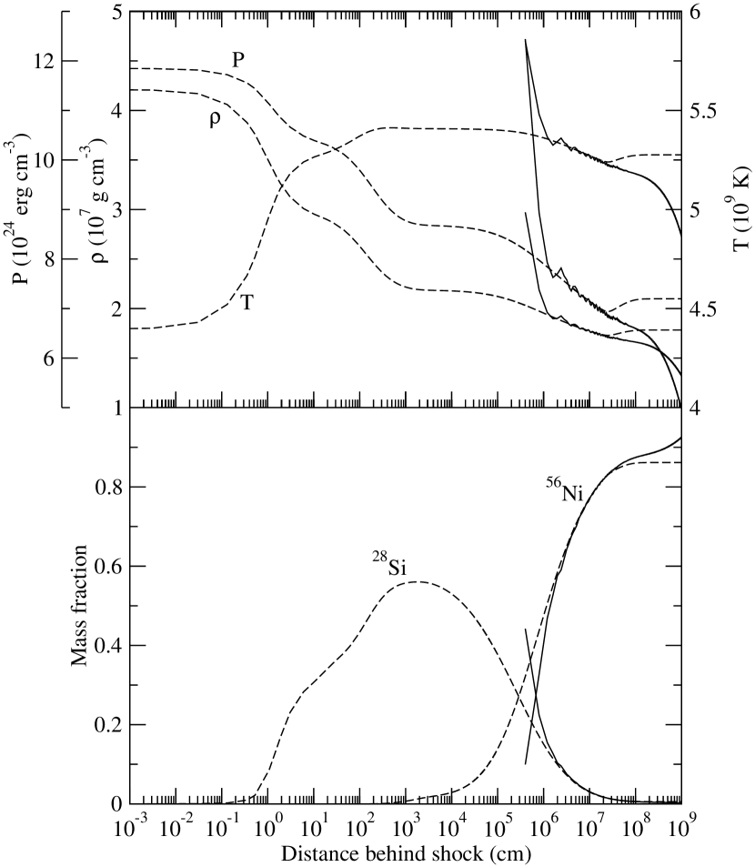
Figure 13.— Comparison of detonation structure at $10^{7}$ g cm^-3 calculated with the ZND formalism (dashed) and simulated with the reactive hydrodynamics methods implemented in Flash (solid) in one dimension. Both methods use the aprox13 enhanced alpha-chain nuclear network.

A fairly large domain was necessary in order for the detonation to come fully into steady state. From Figure 1 the width to completion of burning is nearly $10^{9}$ cm. The domain used was $6.5\times 10^{9}$ cm, with a resolution of $4\times 10^{5}$ cm, and the simulation was run for 5.4 seconds, by which time the detonation nearly consumes the entire domain. The distance behind the shock in the hydrodynamic calculation is computed by taking the distance from the first zone in which reactions are allowed by the shock detection.

We find excellent agreement between the ZND solution and the result of the hydrodynamic simulation despite the entire C and O burning stages being unresolved. After a slight overshoot in all $P$, $\rho$, and $T$ just behind the shock front, the ZND solution is matched within better than 1% out to the pathological point. The hydrodynamic solution then extends smoothly to lower pressures as expected for the unsupported solution. Note that this solution, as expected for an $\alpha$-chain network like aprox13, is somewhat hotter than the more realistic detonation structure given by a larger reaction set discussed in Section 4.3.

Appendix B Example Recorded and Reconstructed Lagrangian Histories

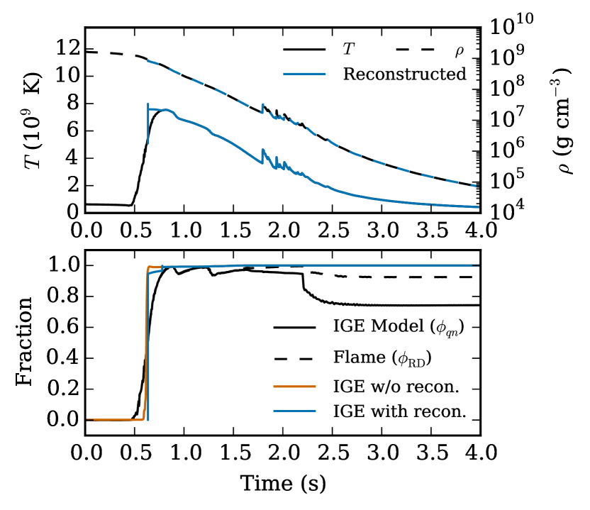
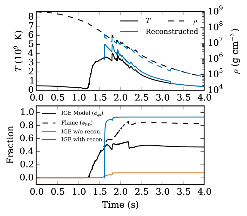
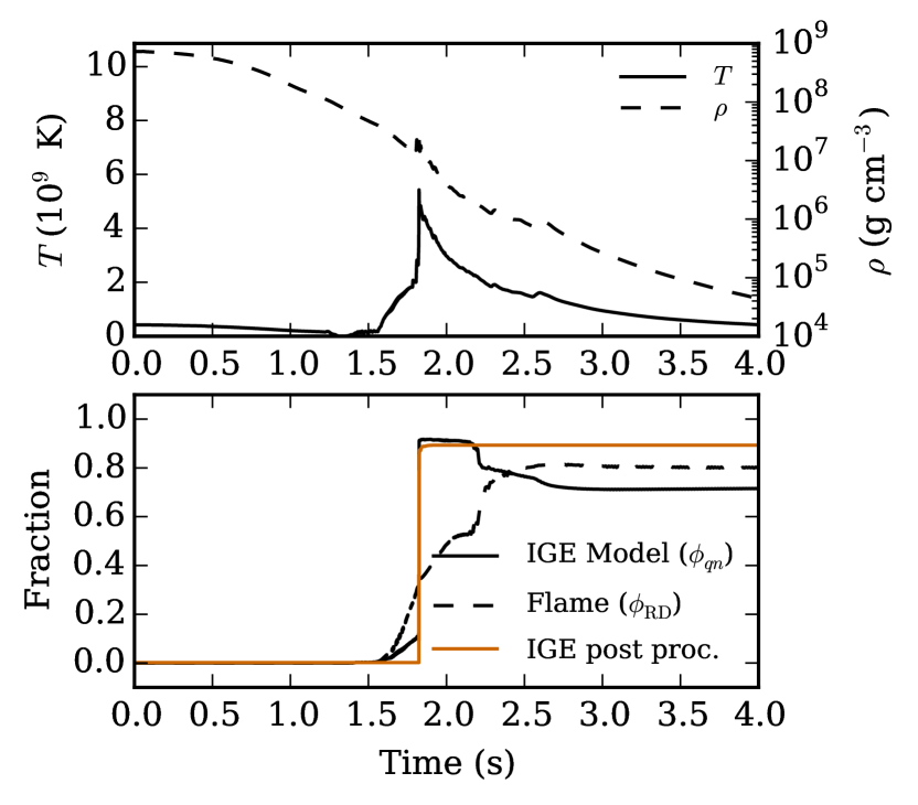
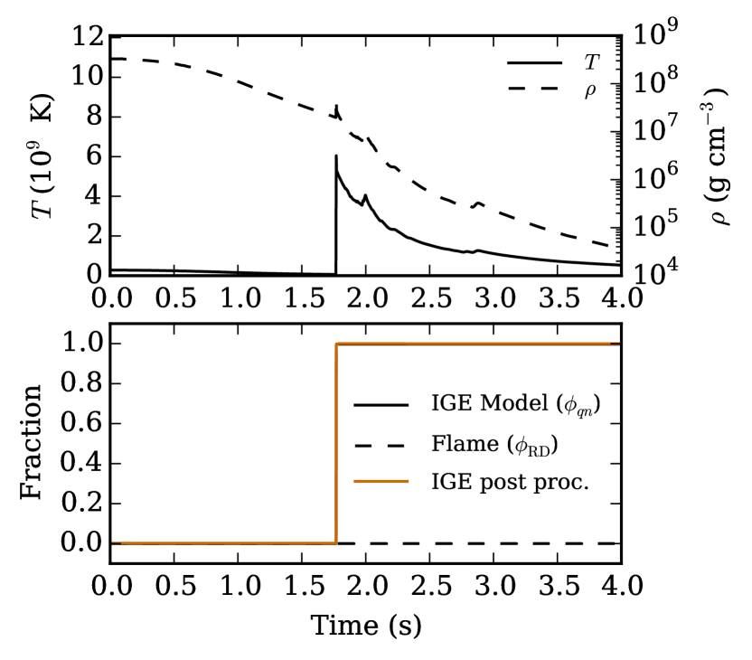
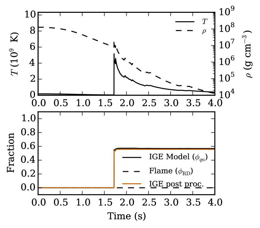
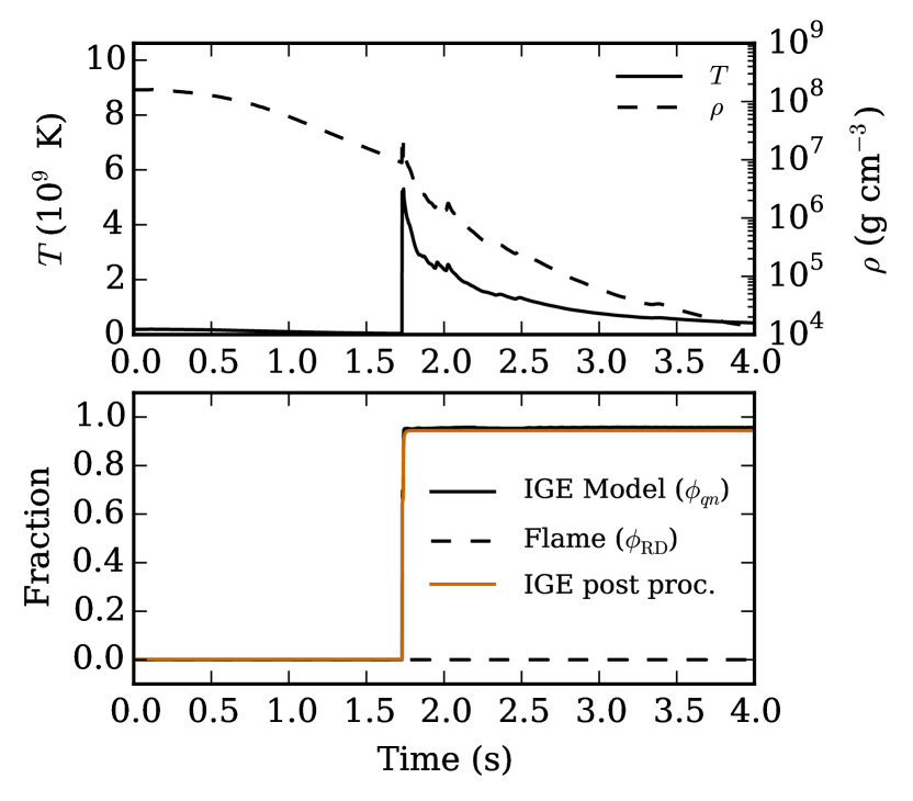
Figure 14.— Example particle histories of various types, see text for individual descriptions. The top panel of each pair shows the temperature (solid, left scale) and density (dashed, right scale) recorded from the simulation (black) and, for deflagration tracks, the reconstructed history (blue). The bottom panel of each pair shows the fraction of IGE, recorded from the burning model in hydrodynamics ($\phi_{qn}$, black) and determined in post-processing with (blue) and without (red) reconstruction reconstruction. Reconstruction is only performed for deflagration tracks. Also shown is the progress variable for the artificial flame, $\phi_{\rm RD}$ (dashed).

In this appendix we present a range of example particle histories from the simulation and the reconstruction obtained from the methods described in the main text. The distribution of tracks among the two burning modes, deflagration and detonation, varies with position in the ejecta, with inner layers having a large deflagration component and outer layers being mostly dominated by detonation products. Histories, both recorded and reconstructed, of $\rho$ and $T$ as well as IGE fraction, which is represented by $\phi_{qn}$ in the burning model and Equation (38) for the post-processed abundances, and $\phi_{\rm RD}$ are shown in Figure 14. These provide examples of the several broad classes of tracks produced by the simulation that we will now describe.

The top left panel in Figure 14 shows a typical time history for a fluid element burned by a deflagration front. The slow, several tenths of a second, rise to peak temperature is replaced in reconstruction by a quick rise followed by a steady decline as the density falls off. The arrival of the detonation shock can be seen at around 1.8 s, and is relatively weak because this location is within the burned material so that the arriving shock is not an active detonation. Some mixing artifacts, show by separation between the IGE fraction for the model and $\phi_{\rm RD}$, are apparent upon arrival of the detonation shock, and can be larger in other cases. This is likely due to the proximity of slightly less burned material and may also indicate a mild mismatch between the advection of the particles and the hydrodynamics when a shock is present. The grid in the simulation is forced to coarsen starting at 2.2 s, after burning has ceased. The numerical mixing associated with the merging of cells can cause either a decrease, as seen here, or an increase of the IGE fraction recorded from the simulation. The best time to compare the IGE fraction produced in post processing with that in the burning model is just before this coarsening. As expected, we find a good but not precise match for deflagration tracks, within 10% or so for this and other similar tracks, as the time the of deflagration is not precisely defined.

The top right panel in Figure 14 shows an example of cases that lead to the largest difference between the yields estimated from the hydrodynamic burning model variables and the post-processed yields. In this deflagration track, when $\phi_{\rm RD}$ passes through 0.5, the density and temperature are still high enough for fairly prompt full burning to Fe-group. This is evidenced both in the recorded $\phi_{qn}$ being similar to $\phi_{\rm RD}$ and the reconstructed post-processing giving an IGE fraction that increases promptly to close to unity. However, as can be seen by the subsequent evolution of the recorded history, $\phi_{qn}$ in the hydrodynamics does not continue to track $\phi_{\rm RD}$. As a result, the hydrodynamic progress variable does not reach near unity as the fluid element passes the rest of the way through the RD front, so that the processing of Si- to Fe-group is more complete in the post-processing. This is a result of the artificially thick and subsonic reaction front, creating an ambiguity in when the burning commences for this fluid element. The fluid state can change (expand) significantly while a particle is passing through the artificial reaction front. Note that when the detonation-produced shock arrives at about 1.8 seconds, it is too weak to cause much further progress in the production of IGE. In some related cases, the shock is strong enough to further produce IGE.

A converse case in which the detonation arrives earlier in the process of artificially thick deflagration can be seen in the middle left panel in Figure 14. Here a particle that has been partially burned by the flame is burned by the detonation. Since the detonation front arrives just before $\phi_{\rm RD}=0.5$, the track is treated as a detonation with its $\rho$, $T$ history directly post-processed, and its IGE yield close to but not quite unity. In this case the deflagration was taking place at low enough density that IGE production was reduced ($\phi_{qn}<\phi_{\rm RD}$), but the detonation created more complete burning. The IGE abundance in the model and post-processing are fairly consistent just before the grid is coarsened at 2.2 seconds.

The right middle panel in Figure 14 shows an example of a fairly clean detonation at higher density ($>10^{7}$ g cm^-3). At pre-detonation densities above $10^{7}$ g cm^-3 burning proceeds fully to IGE in both the burning model and post-processing. A large fraction of the IGE material is produced in this manner.

At lower densities, the burning in the detonation is less complete. The material ejected at higher velocities above about 10 000 km s^-1 is almost all burned in the detonation mode to varying degrees of completeness, with the transition from complete to incomplete near a pre-detonation density of $10^{7}$ g cm^-3. While some of differences are attributable to density, even cases at very similar densities, like the two bottom panels in Figure 14, can lead to different IGE yields depending on the local strength of the detonation. The weaker detonation shown in the left panel may be more curved (Dunkley et al., 2013; Moore et al., 2013) or less fully developed (Townsley et al., 2012). Even for the stronger case, the Si burning is incomplete, giving an IGE fraction just short of unity. Typically in these cases the post processing is quite consistent, within 5% or so, of the IGE yield from the burning model.

Appendix C Sampling Uncertainty

Computation of nucleosynthetic yields by post-processing of Lagrangian histories introduces uncertainty due to the finite sampling of the overall hydrodynamic solution. It is useful to consider this uncertainty separately from the uncertainty due to the finite resolution of the hydrodynamic solution and any uncertainties introduced by assumptions in the models for burning processes discussed in the main body of the paper. Our Lagrangian histories are placed in the hydrodynamic computation by initial position randomly and evenly distributed in mass. This makes the weighting for computation of yields straightforward. As discussed in section 7, we additionally randomly sub-select up to 100 history tracks for each 250 km s^-1 bin in ejection velocity from those available in that bin from the 100,000 tracks included in the hydrodynamic computation.

To estimate the uncertainty due to the finite sampling represented by these discrete tracks, we have computed the standard deviation of the mean for all abundances in each ejection velocity bin. The resulting uncertainty in the major abundances for each velocity bin is shown in Figure 15, intended to be compared directly with the yield profiles shown in Figure 11. The major abundances have uncertainties small enough for the comparisons made in this manuscript, in which we are focusing on the major Fe-group and Si-group yields. For velocity bins between 1,000 and 18,000 km s ^-1, 100 tracks are processed, while for other velocity bins 100 are not available from the 100,000 included in the hydrodynamic computation. The number of available tracks falls to about 40 by 20,000 km s^-1.

If smaller sampling uncertainty is desirable in work using the methods described here, the number of tracks used or the choice of the initial position distribution and weighting of the sampling can be modified to give more samples in a particular portion of the ejecta (e.g. Seitenzahl et al., 2010). As long as the 100 samples in each bin used here is sufficient to accurately characterize the variance of the underlying distribution, the standard deviation of the mean should go as $\propto N^{-1/2}$, where $N$ is the number of tracks. For non-uniform mass sampling, the simple standard deviation of the mean can no longer be used, but it is straightforward to develop a similar measure of uncertainty by estimating the variance of the distribution of yields using appropriate weighting of the samples.

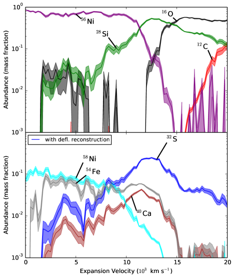
Figure 15.— Profile computed using reconstruction of deflagration histories with colored bands indicating uncertainty due to finite sampling by Lagrangian histories. Uncertainty is taken as the standard deviation of the mean of the abundance over the histories contributing to each velocity bin.

The yield uncertainties can also be propagated in the usual way to the computation of the total yields of all species when the sums over the mass in each ejection velocity bin are performed. The resulting uncertainties are shown in Figure 16 as a fraction of each yield. Most of the uncertainties are in the 2 to 8 percent range, which is comparable to or slightly better than our estimated uncertainty found by comparison to steady-state detonation solutions in section 5. The most neutron-rich isotopes have higher uncertainties because they are produced in a relatively small amount of material, however even a 30% uncertainty is modest in a comparison like that shown in Figure 12, which spans 4 orders of magnitude in abundance. If higher accuracy is desirable for these isotopes in a particular study, more tracks can be included from the regions producing them.

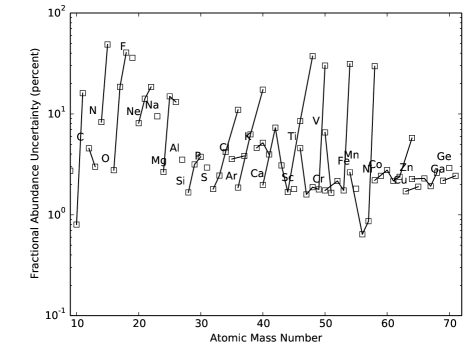
Figure 16.— Uncertainty in total decayed yields due to finite sampling of Lagrangian histories.

Appendix D Tabulated Yields

Table E lists the mass yields of all nuclides with a mass of $10^{-9}M_{\odot}$ or more for our 2D DDT simulation. Masses are listed at two times. Masses in the first column are 4 s after the beginning of the simulation, and those in the second column are after all short-lived radionuclides, defined as those not present in solar abundances, have decayed. At each of these times we show the yields obtained without any reconstruction of the thermal history and with reconstruction of the thermal history near deflagration fronts as described in section 3. The total Fe-group yield, all elements with $Z>22$, is $0.89M_{\odot}$ without reconstruction and $1.0M_{\odot}$ with deflagration reconstruction.

Appendix E Implementation of the burning model

Here we mention several details about the implementation of the burning model outlined in Section 2. By defining the burning model principally by dynamical equations, Equations (25), (26), (27), (31), (34), and (2.2), we intend a clear separation between the physical and numerical aspects of the construction of the model. These dynamical equations are summarized in Table 2, where the operator splitting, discussed below, is also indicated.

First we will address how the various dynamical variables are stored and treated by the hydrodynamical evolution. The fundamental thermodynamic and hydrodynamic variables are the density field, $\rho(\vec{x},t)$, and the mass-specific energy, $\mathcal{E}(\vec{x},t)$. As given in Equation (2), this density is more clearly considered the local baryon density in a particular choice of units. Additional variables, used to describe the two initial abundance fields, $X_{{}^{12}\rm C,i}(\vec{x},t)$ and $X_{{}^{22}\rm Ne,i}(\vec{x},t)$, are stored but are not subject to any source terms. This $X_{{}^{22}\rm Ne,i}$ is used to represent the entire effective neutron excess in the WD material, regardless of the actual nuclides that contribute to this neutron excess. The additional burning state variables include the progress variables, $\phi_{\rm fa}$, $\phi_{\rm qn}$, $\phi_{\rm aq}$, the reaction-diffusion variable $\phi_{\rm RD}$, and the burning state variables $\delta\bar{q}_{\rm qn}$, $\delta Y_{\rm ion,qn}$ and $Y_{e}$. Care was taken in section 2 that all of these burning variables are linear combinations of abundances, and therefore in the absence of source terms evolve hydrodynamically as mass scalars.

Notably $Y_{e}$ is not stored as a partial like $\delta\bar{q}_{qn}$ or $\delta Y_{\rm ion,qn}$. From Equations (20-22), we see that we basically have a choice for each of $Y_{e}$, $Y_{\rm ion}$, and $\bar{q}$ whether to store the partial ”$\delta$” value or the full value. Either can be obtained from the other using the progress variables and initial abundances. In numerical tests we found that storing $\delta Y_{e}$ and constructing $Y_{e}$ when needed proved to not be well-behaved when solving the hydrodynamic step. We believe that this is related to the strong dependence of the pressure on $Y_{e}$ in the highly degenerate material in the interior of the WD. This problem appears to have been wholly ameliorated by using $Y_{e}$ as the advected mass scalar, deriving $\delta Y_{e}$ in order to compute the time evolution given by the source term, and then recomputing $Y_{e}$.

An important feature of our implementation of reactive hydrodynamics is the splitting of the time evolution operator. As described above in Appendix A, our reactive hydrodynamics code, Flash, is operator split between hydrodynamics and energetic source terms. We will also further split our source terms to enable a high-efficiency sub-step integration. In Appendix A the coupled reactions are integrated with a stiff ODE solver that integrates through a hydrodynamical timestep by assuming a constant $T$. For our parameterized model of burning, we will assume that the following quantities are constant during a hydrodynamic step: $\langle\sigma v\rangle_{\rm C+C}$, $\tau_{\rm NSQE}$, $\tau_{\rm NSE}$, $\bar{q}_{\rm NSE}$, $Y_{\rm ion,NSE}$ and $\dot{Y}_{e,\rm NSE}$. These are determined as described in Section 2.2 depending on the proximity to the artificial flame.

Even with these values all assumed to be constant, the burning model is still fairly tightly coupled. In order to separate this coupling, as justified below, we will additionally operator split the burning source terms as shown in Tables 2 and 3. The evolution represented by the Hydro column is computed first, followed by the other columns in Table 2 and then the other columns in Table 3. The final results of each stage is used to compute the evolution of the next. The important aspect of this splitting is that each of the resulting source terms can be analytically integrated through the hydrodynamic timestep, $\Delta t_{\rm H}$. As an example, the C-React operator update is performed as

$$\phi_{\rm fa,C+}=1-\frac{(1-\phi_{\rm fa,C-})}{[1+r_{\rm CC}\,\Delta t(1-\phi_{\rm fa,C-})]}\ ,$$ (E1)

where $\phi_{\rm fa,C-}$ is the value of $\phi_{\rm fa}$ before the C-React operator,and $r_{\rm CC}=\rho X_{{}^{12}\rm C,f}N_{\rm A}\langle\sigma v\rangle_{\rm C+C}$. The other terms besides the flame are all exponential relaxation and can therefore also be analytically integrated. The evolution of $\phi_{\rm RD}$ itself is not directly dependent on the other burning variables.

This operator splitting is effective due to the separation of timescales within the burning model. Generally $\tau_{\rm CC}\ll\tau_{\rm NSQE}\ll\tau_{\rm NSE}$, where each $\tau$ represents an approximate timescale for C+C fusion, oxygen consumption / QSE adjustment, and completion of Si burning. Thus for a given time scale or time step, $\Delta t$, generally only one variable is dynamically active and the others are either nearly frozen out or tracking the dominant variable’s behavior.

Table 1Ejecta yields in $M_{\odot}$

	at 4 seconds		decayed			at 4 seconds		decayed
Nuclide	w/o recon.	defl. recon.	w/o recon.	defl. recon.	Nuclide	w/o recon.	defl. recon.	w/o recon.	defl. recon.
4He	$8.8\times 10^{-3}$	$9.0\times 10^{-3}$	$8.8\times 10^{-3}$	$9.0\times 10^{-3}$	39K	$7.7\times 10^{-5}$	$3.3\times 10^{-5}$	$7.7\times 10^{-5}$	$3.3\times 10^{-5}$
12C	$1.4\times 10^{-3}$	$1.5\times 10^{-3}$	$1.4\times 10^{-3}$	$1.5\times 10^{-3}$	40K	$2.9\times 10^{-8}$	$2.2\times 10^{-8}$	$2.9\times 10^{-8}$	$2.2\times 10^{-8}$
14N	$2.0\times 10^{-9}$	$1.9\times 10^{-9}$	$3.0\times 10^{-9}$	$2.8\times 10^{-9}$	41K	$1.2\times 10^{-8}$	$1.8\times 10^{-8}$	$4.5\times 10^{-6}$	$2.1\times 10^{-6}$
16O	$5.7\times 10^{-2}$	$5.5\times 10^{-2}$	$5.7\times 10^{-2}$	$5.5\times 10^{-2}$	42K	$1.2\times 10^{-8}$	$1.5\times 10^{-8}$
19O	$6.5\times 10^{-9}$				40Ca	$1.7\times 10^{-2}$	$1.6\times 10^{-2}$	$1.7\times 10^{-2}$	$1.6\times 10^{-2}$
19F			$6.8\times 10^{-9}$		41Ca	$4.5\times 10^{-6}$	$2.1\times 10^{-6}$
20Ne	$1.7\times 10^{-3}$	$1.6\times 10^{-3}$	$1.7\times 10^{-3}$	$1.6\times 10^{-3}$	42Ca	$2.6\times 10^{-5}$	$8.7\times 10^{-6}$	$2.6\times 10^{-5}$	$8.8\times 10^{-6}$
21Ne	$1.8\times 10^{-7}$	$2.0\times 10^{-7}$	$1.8\times 10^{-7}$	$2.0\times 10^{-7}$	43Ca	$5.3\times 10^{-8}$	$3.2\times 10^{-8}$	$2.5\times 10^{-7}$	$2.3\times 10^{-7}$
22Ne	$4.5\times 10^{-6}$	$4.5\times 10^{-6}$	$4.5\times 10^{-6}$	$4.5\times 10^{-6}$	44Ca	$5.9\times 10^{-8}$	$4.7\times 10^{-8}$	$3.1\times 10^{-5}$	$3.2\times 10^{-5}$
23Ne	$8.7\times 10^{-9}$	$8.7\times 10^{-9}$			45Ca	$5.2\times 10^{-9}$	$4.7\times 10^{-9}$
22Na	$9.7\times 10^{-9}$	$9.5\times 10^{-9}$			46Ca	$7.2\times 10^{-9}$	$7.3\times 10^{-9}$	$7.2\times 10^{-9}$	$7.3\times 10^{-9}$
23Na	$1.2\times 10^{-5}$	$1.3\times 10^{-5}$	$1.3\times 10^{-5}$	$1.4\times 10^{-5}$	47Ca	$9.2\times 10^{-9}$	$1.3\times 10^{-8}$
24Na	$1.1\times 10^{-7}$	$1.1\times 10^{-7}$			48Ca	$2.4\times 10^{-9}$	$4.4\times 10^{-9}$	$2.4\times 10^{-9}$	$4.4\times 10^{-9}$
23Mg	$1.3\times 10^{-6}$	$1.3\times 10^{-6}$			42Sc	$1.9\times 10^{-8}$	$1.9\times 10^{-8}$
24Mg	$7.2\times 10^{-3}$	$7.0\times 10^{-3}$	$7.2\times 10^{-3}$	$7.0\times 10^{-3}$	43Sc	$2.0\times 10^{-7}$	$2.0\times 10^{-7}$
25Mg	$1.8\times 10^{-5}$	$2.0\times 10^{-5}$	$1.8\times 10^{-5}$	$2.0\times 10^{-5}$	44Sc	$7.5\times 10^{-9}$	$4.5\times 10^{-9}$
26Mg	$3.4\times 10^{-5}$	$3.8\times 10^{-5}$	$3.8\times 10^{-5}$	$4.1\times 10^{-5}$	45Sc	$5.7\times 10^{-8}$	$3.9\times 10^{-8}$	$2.9\times 10^{-7}$	$2.1\times 10^{-7}$
27Mg	$2.8\times 10^{-8}$	$2.9\times 10^{-8}$			46Sc	$6.0\times 10^{-9}$	$4.3\times 10^{-9}$
26Al	$3.5\times 10^{-6}$	$3.2\times 10^{-6}$			47Sc	$8.4\times 10^{-9}$	$8.5\times 10^{-9}$
27Al	$5.3\times 10^{-4}$	$5.2\times 10^{-4}$	$5.4\times 10^{-4}$	$5.2\times 10^{-4}$	48Sc	$6.7\times 10^{-9}$	$6.9\times 10^{-9}$
28Al	$1.3\times 10^{-7}$	$1.4\times 10^{-7}$			49Sc	$2.4\times 10^{-9}$	$2.2\times 10^{-9}$
27Si	$6.5\times 10^{-7}$	$6.7\times 10^{-7}$			44Ti	$3.1\times 10^{-5}$	$3.2\times 10^{-5}$
28Si	$2.4\times 10^{-1}$	$1.6\times 10^{-1}$	$2.4\times 10^{-1}$	$1.6\times 10^{-1}$	45Ti	$2.3\times 10^{-7}$	$1.7\times 10^{-7}$
29Si	$5.3\times 10^{-4}$	$4.5\times 10^{-4}$	$5.3\times 10^{-4}$	$4.5\times 10^{-4}$	46Ti	$1.5\times 10^{-5}$	$5.8\times 10^{-6}$	$1.5\times 10^{-5}$	$5.9\times 10^{-6}$
30Si	$1.1\times 10^{-3}$	$1.1\times 10^{-3}$	$1.1\times 10^{-3}$	$1.1\times 10^{-3}$	47Ti	$3.3\times 10^{-7}$	$1.8\times 10^{-7}$	$1.3\times 10^{-6}$	$1.1\times 10^{-6}$
31Si	$2.6\times 10^{-7}$	$2.6\times 10^{-7}$			48Ti	$3.7\times 10^{-7}$	$3.3\times 10^{-7}$	$4.2\times 10^{-4}$	$4.5\times 10^{-4}$
32Si	$1.7\times 10^{-8}$	$1.7\times 10^{-8}$			49Ti	$2.3\times 10^{-8}$	$1.9\times 10^{-8}$	$3.3\times 10^{-5}$	$3.3\times 10^{-5}$
30P	$4.3\times 10^{-6}$	$3.7\times 10^{-6}$			50Ti	$2.0\times 10^{-7}$	$1.9\times 10^{-7}$	$2.0\times 10^{-7}$	$1.9\times 10^{-7}$
31P	$2.9\times 10^{-4}$	$2.4\times 10^{-4}$	$2.9\times 10^{-4}$	$2.4\times 10^{-4}$	51Ti	$2.7\times 10^{-9}$	$3.1\times 10^{-9}$
32P	$2.1\times 10^{-7}$	$2.1\times 10^{-7}$			52Ti	$2.9\times 10^{-9}$	$3.5\times 10^{-9}$
33P	$1.7\times 10^{-7}$	$2.0\times 10^{-7}$			46V	$9.0\times 10^{-8}$	$9.1\times 10^{-8}$
34P	$1.4\times 10^{-9}$	$1.4\times 10^{-9}$			47V	$9.0\times 10^{-7}$	$8.8\times 10^{-7}$
31S	$4.9\times 10^{-7}$	$4.6\times 10^{-7}$			48V	$8.7\times 10^{-8}$	$5.7\times 10^{-8}$
32S	$1.1\times 10^{-1}$	$8.3\times 10^{-2}$	$1.1\times 10^{-1}$	$8.3\times 10^{-2}$	49V	$2.8\times 10^{-7}$	$2.1\times 10^{-7}$
33S	$2.2\times 10^{-4}$	$1.6\times 10^{-4}$	$2.2\times 10^{-4}$	$1.6\times 10^{-4}$	50V	$2.1\times 10^{-8}$	$2.1\times 10^{-8}$	$2.1\times 10^{-8}$	$2.1\times 10^{-8}$
34S	$1.5\times 10^{-3}$	$9.3\times 10^{-4}$	$1.5\times 10^{-3}$	$9.3\times 10^{-4}$	51V	$5.7\times 10^{-7}$	$5.7\times 10^{-7}$	$1.1\times 10^{-4}$	$1.1\times 10^{-4}$
35S	$1.0\times 10^{-7}$	$9.1\times 10^{-8}$			52V	$4.9\times 10^{-9}$	$4.0\times 10^{-9}$
36S	$1.2\times 10^{-7}$	$1.4\times 10^{-7}$	$1.2\times 10^{-7}$	$1.4\times 10^{-7}$	53V	$2.3\times 10^{-9}$	$1.7\times 10^{-9}$
34Cl	$1.1\times 10^{-7}$	$9.5\times 10^{-8}$			48Cr	$4.2\times 10^{-4}$	$4.5\times 10^{-4}$
35Cl	$8.9\times 10^{-5}$	$4.8\times 10^{-5}$	$8.9\times 10^{-5}$	$4.8\times 10^{-5}$	49Cr	$3.3\times 10^{-5}$	$3.3\times 10^{-5}$
36Cl	$2.9\times 10^{-7}$	$2.7\times 10^{-7}$			50Cr	$4.2\times 10^{-4}$	$3.0\times 10^{-4}$	$4.2\times 10^{-4}$	$3.0\times 10^{-4}$
37Cl	$4.1\times 10^{-7}$	$4.3\times 10^{-7}$	$2.2\times 10^{-5}$	$1.0\times 10^{-5}$	51Cr	$4.5\times 10^{-6}$	$2.5\times 10^{-6}$
38Cl	$1.1\times 10^{-8}$	$1.3\times 10^{-8}$			52Cr	$4.8\times 10^{-4}$	$4.5\times 10^{-4}$	$9.2\times 10^{-3}$	$9.9\times 10^{-3}$
36Ar	$2.0\times 10^{-2}$	$1.7\times 10^{-2}$	$2.0\times 10^{-2}$	$1.7\times 10^{-2}$	53Cr	$4.1\times 10^{-6}$	$4.1\times 10^{-6}$	$1.1\times 10^{-3}$	$1.2\times 10^{-3}$
37Ar	$2.1\times 10^{-5}$	$9.7\times 10^{-6}$			54Cr	$9.2\times 10^{-6}$	$9.1\times 10^{-6}$	$9.2\times 10^{-6}$	$9.1\times 10^{-6}$
38Ar	$9.2\times 10^{-4}$	$3.5\times 10^{-4}$	$9.2\times 10^{-4}$	$3.5\times 10^{-4}$	55Cr	$1.1\times 10^{-8}$	$1.1\times 10^{-8}$
39Ar	$1.9\times 10^{-8}$	$2.0\times 10^{-8}$			56Cr	$2.8\times 10^{-8}$	$3.2\times 10^{-8}$
40Ar	$1.9\times 10^{-8}$	$2.3\times 10^{-8}$	$1.9\times 10^{-8}$	$2.3\times 10^{-8}$	57Cr	$1.3\times 10^{-9}$	$1.4\times 10^{-9}$
41Ar	$6.0\times 10^{-9}$	$8.8\times 10^{-9}$			58Cr	$3.8\times 10^{-9}$	$5.3\times 10^{-9}$
38K	$3.1\times 10^{-7}$	$3.1\times 10^{-7}$			51Mn	$1.0\times 10^{-4}$	$1.1\times 10^{-4}$

Table 1 (cont.)Ejecta yields in $M_{\odot}$ continued

Table 2Division of time evolution into operators

	Hydro	Flame	C-React${}^{\tablenotemark{b}}$	O-consumption${}^{\tablenotemark{b}}$
$\displaystyle\frac{\partial\phi_{\rm RD}}{\partial t}=$	${}-\vec{v}\cdot\nabla\phi_{\rm RD}$	${}+\dot{\phi}_{\rm RD}$${}^{\tablenotemark{a}}$
$\displaystyle\frac{\partial\phi_{fa}}{\partial t}=$	${}-\vec{v}\cdot\nabla\phi_{fa}$	${}+\max\left[0,\dot{\phi}_{\rm RD}\right]$	${}+\rho X_{{}^{12}{\rm C,f}}(1-\phi_{\rm fa})^{2}N_{A}\langle\sigma v\rangle/12$
$\displaystyle\frac{\partial\phi_{\rm aq}}{\partial t}=$	${}-\vec{v}\cdot\nabla\phi_{\rm aq}$			${}+(\phi_{\rm fa}-\phi_{\rm aq})/\tau_{\rm NSQE}$

Table 3Division of time evolution into operators continued

	Hydro	Si-burning${}^{\tablenotemark{b}}$	Energy and Neutronization
$\displaystyle\frac{\partial\phi_{\rm qn}}{\partial t}=$	${}-\vec{v}\cdot\nabla\phi_{\rm qn}$	${}+(\phi_{\rm aq}-\phi_{\rm qn})^{2}/\tau_{\rm NSE}$
$\displaystyle\frac{\partial(\delta Y_{e,n})}{\partial t}=$	${}-\vec{v}\cdot\nabla(\delta Y_{e,n})$	${}+\left[(\phi_{\rm aq}-\phi_{\rm qn})^{2}/\tau_{\rm NSE}\right]Y_{e,0}$	${}+\phi_{\rm qn}\dot{Y}_{e,\rm NSE}$
$\displaystyle\frac{\partial(\delta\bar{q}_{qn})}{\partial t}=$	${}-\vec{v}\cdot\nabla(\delta\bar{q}_{qn})$	${}+\left[(\phi_{\rm aq}-\phi_{\rm qn})^{2}/\tau_{\rm NSE}\right]\bar{q}_{\rm QSE0}$	${}+\left[(\phi_{\rm aq}-\phi_{\rm qn})\bar{q}_{\rm QSE0}+\phi_{\rm qn}\bar{q}_{\rm NSE}-\delta\bar{q}_{qn}\right]/\tau_{\rm NSQE}$ ${}^{\tablenotemark{b}}$
$\displaystyle\frac{\partial(\delta Y_{\rm ion,qn})}{\partial t}=$	${}-\vec{v}\cdot\nabla(\delta Y_{\rm ion,qn})$	${}+\left[(\phi_{\rm aq}-\phi_{\rm qn})^{2}/\tau_{\rm NSE}\right]Y_{\rm ion,QSE0}$	${}+\left[(\phi_{\rm aq}-\phi_{\rm qn})Y_{\rm ion,QSE0}+\phi_{\rm qn}Y_{\rm ion,NSE}-\delta Y_{\rm ion,qn}\right]/\tau_{\rm NSQE}$ ${}^{\tablenotemark{b}}$

References

- Anders & Grevesse (1989) Anders, E., & Grevesse, N. 1989, Geochim. Cosmochim. Acta, 53, 197
- Bloom et al. (2012) Bloom, J. S., Kasen, D., Shen, K. J., et al. 2012, ApJ, 744, L17
- Brachwitz et al. (2000) Brachwitz, F., Dean, D. J., Hix, W. R., et al. 2000, ApJ, 536, 934
- Bravo et al. (2010) Bravo, E., Domínguez, I., Badenes, C., Piersanti, L., & Straniero, O. 2010, ApJ, 711, L66
- Calder et al. (2013) Calder, A. C., Krueger, B. K., Jackson, A. P., & Townsley, D. M. 2013, Frontiers of Physics, 8, 168
- Calder et al. (2002) Calder, A. C., Fryxell, B., Plewa, T., et al. 2002, ApJS, 143, 201
- Calder et al. (2007) Calder, A. C., Townsley, D. M., Seitenzahl, I. R., et al. 2007, ApJ, 656, 313
- Chamulak et al. (2007) Chamulak, D. A., Brown, E. F., & Timmes, F. X. 2007, ApJ, 655, L93
- Chamulak et al. (2008) Chamulak, D. A., Brown, E. F., Timmes, F. X., & Dupczak, K. 2008, ApJ, 677, 160
- Chomiuk et al. (2012) Chomiuk, L., Soderberg, A. M., Moe, M., et al. 2012, ApJ, 750, 164
- Ciaraldi-Schoolmann et al. (2013) Ciaraldi-Schoolmann, F., Seitenzahl, I. R., & Röpke, F. K. 2013, A&A, 559, A117
- Conley et al. (2011) Conley, A., Guy, J., Sullivan, M., et al. 2011, ApJS, 192, 1
- Domínguez & Khokhlov (2011) Domínguez, I., & Khokhlov, A. 2011, ApJ, 730, 87
- Döring (1943) Döring, W. 1943, AnP, 435, 421
- Dubey et al. (2012) Dubey, A., Daley, C., ZuHone, J., et al. 2012, ApJS, 201, 27
- Dubey et al. (2009) Dubey, A., Reid, L. B., Weide, K., et al. 2009, ArXiv e-prints, arXiv:0903.4875
- Dunkley et al. (2013) Dunkley, S. D., Sharpe, G. J., & Falle, S. A. E. G. 2013, MNRAS, 431, 3429
- Fickett & Davis (1979) Fickett, W., & Davis, W. C. 1979, Detonation (Berkeley: University of California Press)
- Filippenko (1997) Filippenko, A. V. 1997, ARA&A, 35, 309
- Fink et al. (2010) Fink, M., Röpke, F. K., Hillebrandt, W., et al. 2010, A&A, 514, A53
- Fink et al. (2014) Fink, M., Kromer, M., Seitenzahl, I. R., et al. 2014, MNRAS, 438, 1762
- Fryxell et al. (2000) Fryxell, B., Olson, K., Ricker, P., et al. 2000, ApJS, 131, 273
- Fryxell et al. (1989) Fryxell, B. A., Müller, E., & Arnett, D. 1989, MPIA Technical Report
- Fuller et al. (1985) Fuller, G. M., Fowler, W. A., & Newman, M. J. 1985, ApJ, 293, 1
- Gamezo et al. (1999) Gamezo, V. N., Wheeler, J. C., Khokhlov, A. M., & Oran, E. S. 1999, ApJ, 512, 827
- Hillebrandt & Niemeyer (2000) Hillebrandt, W., & Niemeyer, J. C. 2000, ARA&A, 38, 191
- Höflich et al. (1995) Höflich, P., Khokhlov, A. M., & Wheeler, J. C. 1995, ApJ, 444, 831
- Jackson et al. (2010) Jackson, A. P., Calder, A. C., Townsley, D. M., et al. 2010, ApJ, 720, 99
- Jackson et al. (2014) Jackson, A. P., Townsley, D. M., & Calder, A. C. 2014, ApJ, 784, 174
- Jordan et al. (2008) Jordan, IV, G. C., Fisher, R. T., Townsley, D. M., et al. 2008, ApJ, 681, 1448
- Jordan et al. (2012a) Jordan, IV, G. C., Perets, H. B., Fisher, R. T., & van Rossum, D. R. 2012a, ApJ, 761, L23
- Jordan et al. (2012b) Jordan, IV, G. C., Graziani, C., Fisher, R. T., et al. 2012b, ApJ, 759, 53
- Khokhlov (1983) Khokhlov, A. M. 1983, Soviet Astronomy Letters, 9, 160
- Khokhlov (1989) —. 1989, MNRAS, 239, 785
- Khokhlov (1991) —. 1991, A&A, 245, 114
- Khokhlov (2000) —. 2000, ApJ, submitted, astro-ph/0008463
- Kim et al. (2013) Kim, Y., Jordan, IV, G. C., Graziani, C., et al. 2013, ApJ, 771, 55
- Krueger et al. (2012) Krueger, B. K., Jackson, A. P., Calder, A. C., et al. 2012, ApJ, 757, 175
- Krueger et al. (2010) Krueger, B. K., Jackson, A. P., Townsley, D. M., et al. 2010, ApJ, 719, L5
- Langanke & Martínez-Pinedo (2001) Langanke, K., & Martínez-Pinedo, G. 2001, At. Data Nucl. Data Tables, 79, 1
- Li et al. (2011) Li, W., Bloom, J. S., Podsiadlowski, P., et al. 2011, Nature, 480, 348
- Livne & Arnett (1995) Livne, E., & Arnett, D. 1995, ApJ, 452, 62
- Long et al. (2014) Long, M., Jordan, IV, G. C., van Rossum, D. R., et al. 2014, ApJ, 789, 103
- Maeda et al. (2010) Maeda, K., Röpke, F. K., Fink, M., et al. 2010, ApJ, 712, 624
- Mazzali et al. (2008) Mazzali, P. A., Sauer, D. N., Pastorello, A., Benetti, S., & Hillebrandt, W. 2008, MNRAS, 386, 1897
- Meakin et al. (2009) Meakin, C. A., Seitenzahl, I., Townsley, D., et al. 2009, ApJ, 693, 1188
- Miles et al. (2015) Miles, B. J., van Rossum, D. R., Townsley, D. M., et al. 2015, ApJ submitted, (arXiv:1508.05961)
- Moore et al. (2013) Moore, K., Townsley, D. M., & Bildsten, L. 2013, ApJ, 776, 97
- Nomoto et al. (1984) Nomoto, K., Thielemann, F.-K., & Yokoi, K. 1984, ApJ, 286, 644
- Nugent et al. (2011) Nugent, P. E., Sullivan, M., Cenko, S. B., et al. 2011, Nature, 480, 344
- Oda et al. (1994) Oda, T., Hino, M., Muto, K., Takahara, M., & Sato, K. 1994, A. Data Nucl. Data Tables, 56, 231
- Phillips (1993) Phillips, M. M. 1993, ApJ, 413, L105
- Piro & Bildsten (2008) Piro, A. L., & Bildsten, L. 2008, ApJ, 673, 1009
- Press et al. (1992) Press, W. H., Teukolsky, S. A., Vetterling, W. T., & Flannery, B. P. 1992, Numerical Recipes in FORTRAN (Cambridge: Cambridge Univerisity Press)
- Röpke (2006) Röpke, F. K. 2006, in Reviews in Modern Astronomy, Vol. 19, Reviews in Modern Astronomy, ed. S. Roeser, 127
- Scalzo et al. (2014) Scalzo, R., Aldering, G., Antilogus, P., et al. 2014, MNRAS, 440, 1498
- Seitenzahl et al. (2011) Seitenzahl, I. R., Ciaraldi-Schoolmann, F., & Röpke, F. K. 2011, MNRAS, 414, 2709
- Seitenzahl et al. (2009a) Seitenzahl, I. R., Meakin, C. A., Townsley, D. M., Lamb, D. Q., & Truran, J. W. 2009a, ApJ, 696, 515
- Seitenzahl et al. (2010) Seitenzahl, I. R., Röpke, F. K., Fink, M., & Pakmor, R. 2010, MNRAS, 407, 2297
- Seitenzahl et al. (2009b) Seitenzahl, I. R., Townsley, D. M., Peng, F., & Truran, J. W. 2009b, Atomic Data and Nuclear Data Tables, 95, 96
- Seitenzahl et al. (2013) Seitenzahl, I. R., Ciaraldi-Schoolmann, F., Röpke, F. K., et al. 2013, MNRAS, 429, 1156
- Sharpe (1999) Sharpe, G. J. 1999, MNRAS, 310, 1039
- Sharpe (2001) —. 2001, MNRAS, 322, 614
- Stehle et al. (2005) Stehle, M., Mazzali, P. A., Benetti, S., & Hillebrandt, W. 2005, MNRAS, 360, 1231
- Timmes (1999) Timmes, F. X. 1999, ApJS, 124, 241
- Timmes & Arnett (1999) Timmes, F. X., & Arnett, D. 1999, ApJS, 125, 277
- Timmes et al. (2003) Timmes, F. X., Brown, E. F., & Truran, J. W. 2003, ApJ, 590, L83
- Timmes & Woosley (1992) Timmes, F. X., & Woosley, S. E. 1992, ApJ, 396, 649
- Timmes et al. (2000) Timmes, F. X., Zingale, M., Olson, K., et al. 2000, ApJ, 543, 938
- Townsley et al. (2007) Townsley, D. M., Calder, A. C., Asida, S. M., et al. 2007, ApJ, 668, 1118
- Townsley et al. (2009) Townsley, D. M., Jackson, A. P., Calder, A. C., et al. 2009, ApJ, 701, 1582
- Townsley et al. (2012) Townsley, D. M., Moore, K., & Bildsten, L. 2012, ApJ, 755, 4
- Travaglio et al. (2004) Travaglio, C., Hillebrandt, W., Reinecke, M., & Thielemann, F.-K. 2004, A&A, 425, 1029
- Vladimirova et al. (2006) Vladimirova, N., Weirs, G., & Ryzhik, L. 2006, Combust. Theory Modelling, 10, 727
- von Neumann (1942) von Neumann, J. 1942, Tech. Rep. OSRD-549, National Defense Research Committee
- von Neumann (1963) —. 1963, in John von Neumann: Collected Works, 1903–1957, Vol. 6 (Oxford: Pergamon), 178
- Willcox et al. (2016) Willcox, D. E., Townsley, D. M., Calder, A. C., Denissenkov, P. A., & Herwig, F. 2016, ApJ submitted, (arXiv:1602.06356)
- Zel’dovich (1940) Zel’dovich, Y. 1940, ZhETF, 10, 542