On thermodynamic inconsistencies in several photosynthetic and solar cell models and how to fix them

Abstract

We analyze standard theoretical models of solar energy conversion developed to study solar cells and photosynthetic systems. We show that the assumption that the energy transfer to the reaction center/electric circuit is through a decay rate or “sink”, is in contradiction with the second law of thermodynamics. We put forward a thermodynamically consistent alternative by explicitly considering parts of the reaction center/electric circuit and by employing a Hamiltonian transfer. The predicted energy transfer by the new scheme differs from the one found using a decay rate, casting doubts on the validity of the conclusions obtained by models which include the latter.

Light-harvesting organism and solar cells convert thermal photons from the sun, into useful energy such as ATP or electric power Blankenship (2013); Nelson (2003); Würfel and Würfel (2009). Understanding and improving these processes may led to more efficient ways to produce clean energy (see Blankenship et al. (2011) and references within). These systems are effectively heat engines Alicki et al. (2016); Einax and Nitzan (2014); Kondepudi and Prigogine (2014); Gelbwaser-Klimovsky et al. (2015) because they transform a heat flow into power (useful energy). Therefore, they are constrained by the laws of thermodynamics Shockley and Queisser (1961); Blankenship et al. (2011); Landsberg and Tonge (1980); Knox and Parson (2007); Knox (1969); Parson (1978); Ross and Calvin (1967); Alicki and Gelbwaser-Klimovsky (2015) which set a fundamental efficiency bound based on the distinction between the two forms of energy exchange: heat flow and power. These two are not interchangeable: in a cyclic process, power may be totally converted into heat flow, but the opposite is forbidden by the second law of thermodynamics Kondepudi and Prigogine (2014); Gelbwaser-Klimovsky et al. (2013); Gelbwaser-Klimovsky and Kurizki (2014).

A key for understanding the efficiency and the power produced by solar cells and plants, is the development of microscopical models of the energy absorption, transmission and storage. Previous works have proposed that effects such environment assisted quantum transport Mohseni et al. (2008); Rebentrost et al. (2009); Plenio and Huelga (2008), coherent nuclear motion Novoderezhkin et al. (2004); Killoran et al. (2014), as well as quantum coherences Dorfman et al. (2013); Scully et al. (2011); Creatore et al. (2013); Fassioli et al. (2010), play an important role in the enhancement of the energy conversion.

For practical computational and theoretical reasons, models have been restricted to the study of specific subsystems. It is customary to study photosynthetic complexes coupled to "traps" or "sinks" that represent the reaction center where exciton dissociation occurs Mohseni et al. (2008); Plenio and Huelga (2008); Rebentrost et al. (2009). Similar models have been employed for the study of exciton absorption and transport in, e.g., organic solar cells Alharbi and Kais (2015); Cao and Silbey (2009); Creatore et al. (2013); Dorfman et al. (2013); Killoran et al. (2014); Scully et al. (2011).

Here we show that if not careful, the introduction of sinks and traps leads to violations of the second law of thermodynamics. These violations are a reason of concern for the validity of the models that have been employed to date. To shed light on the issue and to provide a simple to understand situation, we introduce a toy model to study this approximation and put forward a thermodynamically consistent version of it. This model could be used as the basis for more elaborate solar cell and plant microscopic models. Finally, we show that the output power of the thermodynamically-consistent version of the model can differ substantially to the simple trap or sink models.

Second law of thermodynamics

The standard thermodynamic models for solar energy conversion are comprised by a system, S, that interacts with different thermal baths and transforms the solar energy into chemical energy or electric current. Here we analyze two types of models: donor-acceptor models, where S is composed of four to five levels. These models have been applied for studying solar cells Creatore et al. (2013); Scully et al. (2011) as well as photosynthetic systems Dorfman et al. (2013) (see Figure 1a); or models of the celebrated Fenna-Matthews-Olson (FMO) complex models, where S includes seven bacteriochlorophyll, each of them described by a single energy state Alharbi and Kais (2015); Cao and Silbey (2009); Killoran et al. (2014); Mohseni et al. (2008); Plenio and Huelga (2008); Rebentrost et al. (2009) (see Figure 1b). In both cases, the energy conversion process is composed of the following explicit or implicit steps: i) Light absorption. The system, S, absorbs hot photons coming from the sun. The temperature of the photon is $T_{abs}$ and $J_{abs}$ is the heat flow between the hot photons and S; ii) Energy transfer. The absorbed energy is transmitted between different states of the S. The number of states and allowed transitions varies from case to case. During this stage some energy is lost through a heat current, $J_{loss}$, to a vibrational bath at room temperature $T_{loss}$ (material photons for solar cells Würfel and Würfel (2009); Nelson (2003) or protein modes for photosynthetic systems Blankenship (2013)); iii) Power extraction. A decay rate that represents an irreversible energy flow to an external system, work reservoir. The latter is generally not explicitly considered. For photosynthetic models this last stage, involves the decay to a sink or trap, together with an energy transfer to the RC and its subsequent transformation into chemical energy. In the case of solar cells, the energy flow is the electric power that runs through the circuit.

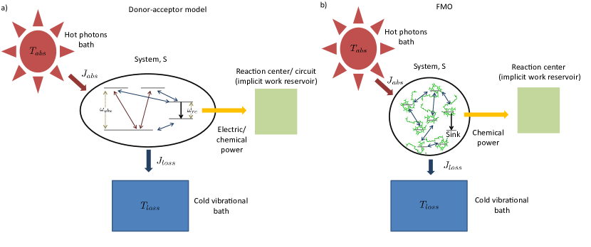
Figure 1: (Color online) Solar energy conversion models: a) donor-acceptor model; b) FMO model. In both cases the allowed transitions are shown only for illustration purposes and may vary between different models.

The dynamics of these systems is constrained by the second law of thermodynamics, through the entropy production inequality Spohn (1978); Gelbwaser-Klimovsky et al. (2015),

$$\sigma=\dot{S}(\rho_{s})-\frac{J_{abs}}{T_{abs}}-\frac{J_{loss}}{T_{loss}}\geq 0,$$ (1)

where $\sigma$ is the entropy production, $\rho_{s}$ is S density matrix and $\dot{S}$ is the derivative over time of the Von-Neumann entropy Breuer and Petruccione (2002). For the heat currents, as wells as for the power, we use the sign convention that energy flowing to and from S is positive and negative respectively. Models with artificial sinks could be envisioned as systems that transfer energy to a zero-temperature bath. This will justified the addition of an extra term on the r.h.s of Eq. (1). In such circumstances the efficiency of the system, in principle can be up to 100%. Nevertheless, solar cells and plants must obey the same thermodynamic bound as a heat engine operating between thermal baths at the temperatures of the sun and the vibrational bath, which are 6000k and 300k respectively and therefore bounded to $95\%$. This is a maximum absolute bound based solely on the temperatures. In more elaborate models, the bound is even lower Shockley and Queisser (1961); Blankenship et al. (2011); Landsberg and Tonge (1980); Knox and Parson (2007); Knox (1969); Parson (1978); Ross and Calvin (1967); Alicki and Gelbwaser-Klimovsky (2015).

In the case of a steady state flux of solar energy into S, the state of S on average does not change, and the second law, Eq. 1, simplifies to

$$\frac{-J_{loss}}{J_{abs}}\geq\frac{T_{loss}}{T_{abs}},\quad J_{abs}>0,$$

$$\frac{-J_{loss}}{J_{abs}}\leq\frac{T_{loss}}{T_{abs}},\quad J_{abs}<0.$$ (2)

The donor/acceptor models studied in Dorfman et al. (2013); Scully et al. (2011); Creatore et al. (2013); Fassioli et al. (2010), analyze the solar energy conversion at steady state, and their heat currents ratio has the form (see SI):

$$\frac{-J_{loss}}{J_{abs}}=1-\frac{\omega_{rc}}{\omega_{abs}},$$ (3)

where $\omega_{abs}$ is the energy of the absorbed photons and $\omega_{rc}$ is the energy of the excitation transferred to the RC/circuit (work reservoir) (see Figure 1a). In all these models, the signs of the currents are independent of the parameters, $J_{loss}<0$ and $J_{abs}>0$ (see SI).

As shown in Figure 2a, for $1-\frac{T_{loss}}{T_{abs}}\leq\frac{\omega_{rc}}{\omega_{abs}},$ these models violate the second law of thermodynamics. Realistic model parameters may well fall outside of this range. This does not exclude the fact that the model is both inconsistent and potentially leading to artificial results. As we show below, the power predicted by a thermodynamically consistent model differs from the simple sink or trap models.

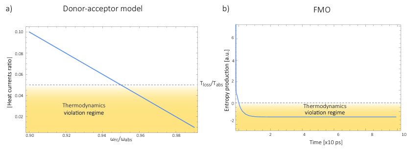
Figure 2: (Color online) Violation of thermodynamics by models of solar energy conversion. a) Absolute value of the heat currents ratio as function of frequency ratio for the steady state models on references Dorfman et al. (2013); Scully et al. (2011); Creatore et al. (2013); Fassioli et al. (2010). For large $\omega_{rc}$, see Eqs. (2) and (3), these models break the second law of thermodynamics; b) Entropy production as a function of time for FMO models Alharbi and Kais (2015); Cao and Silbey (2009); Killoran et al. (2014); Mohseni et al. (2008); Plenio and Huelga (2008); Rebentrost et al. (2009); Caruso et al. (2009). In both graphs the shaded area represents a regime forbidden by thermodynamics.

Figure 2b shows the entropy production (Eq.1) as function of time for standard sink or trap models of the FMO complex Alharbi and Kais (2015); Cao and Silbey (2009); Killoran et al. (2014); Mohseni et al. (2008); Plenio and Huelga (2008); Rebentrost et al. (2009); Caruso et al. (2009). A simplified model is used for the antenna (a two level system), which is coupled to the FMO. The energy is transferred to the RC (work reservoir) through a decay term (see Figure 1b and SI). In this scenario the dynamics outside the steady state is considered. For these models, there is not a simple analytical expression such as Eq. 3, therefore we use a standard numeric simulation based on a Lindblad equation Davies (1974); Gorini et al. (1976); Lindblad (1976). As seen in Figure 2b, these models also violate the second law of thermodynamics. Details of our model can be found in the SI.

Thermodynamically-consistent model

The assumption in the trap or sink models that the energy transfer to the RC/circuit is based solely on a relaxation process, introduces an inconsistency with thermodynamics. Even though physically this energy flow is power, a decay rate effectively represents a heat flow to a thermal bath. This is the root of the inconsistency. Here we use a toy model to clarify this point and put forward an alternative that could serve as basis to correctly model these systems. We compare between two possible energy transfers schemes to the RC/circuit: i) standard decay; ii) Hamiltonian transfer.

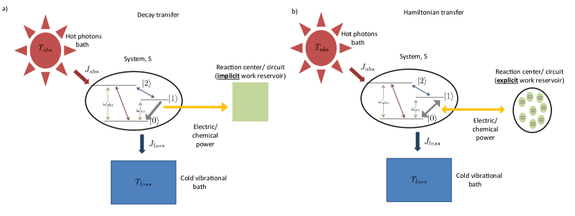
Figure 3: (Color online) A toy model used to study different energy transfer schemes: decay rate (left); Hamiltonian transfer (right).

As S, we consider a three level system as shown in Figure 3. The absorption of a photon causes an excitation transfer between $|0\rangle$ and $|2\rangle$, whereas phonons are emitted by transitions from $|2\rangle$ to $|1\rangle$. Finally, the cycle is closed by a transition between $|1\rangle$ and $|0\rangle$, and the energy difference is transferred to the RC/circuit.

For both schemes the S-bath Hamiltonian is

$$H_{s}+H_{B}+H_{SB}.$$ (4)

The S Hamiltonian, in natural units ($\hbar=1$ and $k_{B}=1$) is

$$H_{S} = \omega_{abs}|2\rangle\langle 2|+\frac{\omega_{rc}}{2}\left(|1\rangle\langle 1|-|0\rangle\langle 0|\right)$$ (5)

and $H_{B}=H_{Photons}+H_{Phonons}$ are the photon and phonon bath free Hamiltonian. Both baths are in thermal equilibrium at temperatures $T_{abs}$ and $T_{loss},$ respectively. The S-bath interaction is governed by

$$H_{SB}=\sum_{\lambda}g_{h,\lambda}\left(|2\rangle\langle 0|a_{\lambda}+|0\rangle\langle 2|a_{\lambda}^{\dagger}\right)$$

$$+\sum_{\lambda}g_{c,\lambda}\left(|2\rangle\langle 1|b_{\lambda}+|1\rangle\langle 2|b_{\lambda}^{\dagger}\right),$$ (6)

where $a_{\lambda},$$a_{\lambda}^{\dagger}$ ($b_{\lambda},$$b_{\lambda}^{\dagger}$) are the annihilation and creation operator of photons (phonons) modes. We assume that the baths are Markovian and are weakly coupled to S Breuer and Petruccione (2002). For the sake of simplicity, we assume that the zero temperature decay rates Gordon et al. (2009) of both baths are the same as the transfer rate to the RC/circuit, $\Gamma_{h}=\Gamma_{c}=\Gamma$ (see SI).

i) Decay transfer

The standard relaxation scheme is a decay rate between $|1\rangle$ and $|0\rangle$,

$$H_{trans}^{Dec}=\sqrt{\Gamma}|0\rangle\langle 1|,$$ (7)

where the RC/circuit is not explicitly included;

ii) Hamiltonian transfer

An alternative to the model above is to explicitly include at least part of the RC/circuit, which plays the role of the work reservoir. In photosynthetic systems, the last stage on the reaction center is the transfer of electrons to the $Q_{B}$ quinone, that once is full, migrates to further proceed with the ATP production Jones (2009). This quinone is replaced by an empty one from a quinone pool. Inspired by this process, we construct a toy model of the work reservoir that could be a guideline for more complicated photosynthetic or solar cells models. It consists of a collection of independent and identical two level systems (TLS). Each of them represents a quinone in a photosynthetic system or an electrode site in a solar cell. The ground state corresponds to an empty quinone/site, and the excited state to a “full” quinone/site. Furthermore, we assume that there are always empty quinones/sites available to accept an electron. Thus, the number of quinones/sites, $j,$ is always much larger than the number of electrons $c^{\dagger}c$, $j\gg c^{\dagger}c$. This assumption is equivalent to the thermodynamic limit taken in the Holstein-Primakoff procedure Holstein and Primakoff (1940); Emary and Brandes (2004), which allows to describe the collection of quinones/sites as a single harmonic oscillator (HO). Therefore, we can write the work reservoir and transfer Hamiltonian as (see SI)

$$H_{trans}^{Ham}=\sqrt{\Gamma}\left(c|1\rangle\langle 0|+c^{\dagger}|0\rangle\langle 1|\right)+\omega_{rc}(c^{\dagger}c-j),$$ (8)

where $c$, $c^{\dagger}$ are the annihilation and creation operator of the HO. Furthermore, for the sake of simplicity we assume that the HO is resonant with the $|1\rangle\leftrightarrow|0\rangle$ transition and that is weakly coupled to S, $\omega_{rc}\gg\Gamma$.

In order to find the energy that is being transferred, in both schemes we first solve the dynamic equations. For this we use the standard Born-Markov approximation Breuer and Petruccione (2002) and write the Lindblad equations for (see SI): i) the three level system in the case of the decay rate scheme; ii) the three level system and the HO for the Hamiltonian transfer scheme, which are at product state due to the weak coupling between them. For both schemes, we analyze the energy transfer at the three level system steady state.

i) For the decay transfer the excitations rate to the RC/circuit is $\Gamma\rho^{ss}_{11},$ and the power is (see SI)

$$P^{Dec}=-\omega_{rc}\Gamma\rho_{11}^{ss},$$

$$\rho_{11}^{ss}=\frac{1}{1+2e^{\left(\omega_{abs}+\frac{\omega_{rc}}{2}\right)/T_{abs}}},$$ (9)

where $\rho_{11}^{ss}$ is the steady state population of level $|1\rangle$. Power is always extracted ($P^{Dec}<0)$, even if the temperatures are the same, $T_{abs}=T_{loss}$. This is in contradiction with thermodynamics, which forbids cyclic power extraction in the presence of a single temperature. A further evidence of the violation of thermodynamics is the combination between the temperature independence of the heat currents ratio and the positivity of $J_{abs}^{Dec}$ (Eqs. (2) and (3)),

$$\frac{-J_{loss}^{Dec}}{J_{abs}^{Dec}}=\frac{2\omega_{abs}-\omega_{rc}}{2\omega_{abs}+\omega_{rc}},$$

$$J_{abs}^{Dec}=\left(\omega_{abs}+\frac{\omega_{rc}}{2}\right)\Gamma\rho_{11}^{ss}>0.$$ (10)

For $\frac{2\omega_{abs}-\omega_{rc}}{2\omega_{abs}+\omega_{rc}}<\frac{T_{loss}}{T_{abs}}$ the model breaks the second law of thermodynamics, Eq. (2).

ii) The power extraction for the Hamiltonian transfer differs from $P^{Dec}$ (see SI),

$$P^{Ham}=-\omega_{rc}\langle\dot{n}\rangle=-\omega_{rc}(s-r),$$ (11)

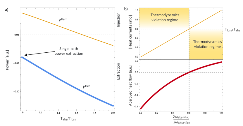
Figure 4: (Color online) a) Predicted power extraction for the decay ($P^{Dec}$, thick blue line) and the Hamiltonian ($P^{Ham},$ thin yellow line) transfer schemes. The former predicts power extraction, $P^{Dec}<0$, from a single bath ($\frac{T_{loss}}{T_{abs}}=1$), while the latter does not ($P^{Ham}>0$). b) Absolute value of the heat currents ratio (yellow thin line) for the Hamiltonian transfer scheme (top). The sign change of $J_{abs}^{Ham},$ (bottom, thick red line) splits the regions forbidden by thermodynamics (shaded areas), preventing its violation. In contrast, for the decay transfer scheme, $J_{abs}^{Dec}$ is always positive, preventing the thermodynamically forbidden region splitting and placing the heat currents ratio in a thermodynamically forbidden region (see Figure 2a).

$\langle\dot{n}\rangle$ is the HO population change. We have assumed an ideal case, where all the energy flow to the HO is considered as power, which just represents a maximum bound Gelbwaser-Klimovsky et al. (2013); Gelbwaser-Klimovsky and Kurizki (2014). The heat currents are (see SI)

$$J_{abs}^{Ham}=\left(\omega_{abs}+\frac{\omega_{rc}}{2}\right)(s-r),$$

$$J_{loss}^{Ham}=-\left(\omega_{abs}-\frac{\omega_{rc}}{2}\right)(s-r)$$ (12)

and

$$s-r=$$

$$K_{1}\left(e^{-\left(\omega_{abs}+\frac{\omega_{rc}}{2}\right)/T_{abs}}-e^{-\left(\omega_{abs}-\frac{\omega_{rc}}{2}\right)/T_{loss}}\right),$$ (13)

where $K_{1}$ is always positive and depends on the couplings to baths (see SI). In contrast to the decay transfer scheme, in this case power is extracted, $P^{Ham}<0$, only for certain combination of parameters,

$$\frac{T_{loss}}{T_{abs}}<\frac{2\omega_{abs}-\omega_{rc}}{2\omega_{abs}+\omega_{rc}}$$ (14)

and power can not be extracted if both temperatures are the same. Further divergences between $P^{Dec}$ and $P^{Ham}$ can be seen in Figure 4a.

Figure 4b shows that the heat currents ratio of the Hamiltonian transfer scheme complies with the second law of thermodynamics (see Eq 2). The thermodynamic violation regime splits due to $J_{abs}^{Ham}$ sign change. Although for positive $J_{abs}^{Ham}$, the absolute value of the heat currents ratio should be larger than the temperatures ratio, for negative $J_{abs}^{Ham}$, it should be smaller. The lack of sign change for $J_{abs}^{Dec}$, prevents the splitting of the thermodynamic violation regime, placing the heat currents ratio in a thermodynamically forbidden region (see Figure 2a).

Conclusions

We have analyzed several models used for describing energy absorption and transmission both in solar cells and in photosynthetic systems such as the FMO complex. We have shown that the use of sinks, traps or any artificial relaxation process in order to describe the energy transfer to a further stage (the reaction center in photosynthetic systems or the electric circuit in a solar cell) introduces a contradiction with the second law of thermodynamics. This invalidates several models currently used to study solar energy conversion, casting doubts regarding their conclusions. These includes the role of coherences, environment assisted quantum transport, coherent nuclear motion and the presence of quantum effects in photosynthesis, among others. We do not argue against the existence of those effects in the conversion of solar energy. But they should be verified using thermodynamically consistent models.

We have further proposed how to correctly analyze these systems. We show this in a thermodynamically consistent toy model that explicitly describes parts of the RC/circuit and uses a Hamiltonian term to describe the energy transfer instead of a decay rate. The predicted transmitted energy greatly differs between these two alternatives (see Figure 4a), highlighting the need to review the conclusions derived by thermodynamically inconsistent models.

Supplementary information

I Energy conversion models

We derive the evolution equations for some examples of two types of energy conversion models. The results of this section are used to generate Figure 2 in the main text, as well as Eq. 3. Unless otherwise stated, we assume $\hbar=k_{b}=1$.

I.1 Donor-acceptor models

As examples of these models, we analyze below two particular donor-acceptor models that use a decay transfer scheme. This kind of analysis may be expanded to models that include coherent vibronic evolution such as the proposed on Killoran et al. (2014).

1) We consider the biological quantum heat engine model proposed on Dorfman et al. (2013) (see in particular Eqs. S34-S37 on Dorfman et al. (2013)) . It consists of a four level system coupled to a hot bath, a cold bath, and to the reaction center/circuit (also termed “the load”). $T_{h(c)}$ is the hot (cold) bath temperature. The different decay rates are shown in Figure S1. The equations of motion are

$$\dot{\rho}_{aa}=-\gamma_{c}\left[\left(1+\bar{n}_{c}\right)\rho_{aa}-\bar{n}_{c}\rho_{\alpha\alpha}\right]-\gamma_{h}\left[\left(1+\bar{n}_{h}\right)\rho_{aa}-\bar{n}_{h}\rho_{bb}\right],$$

$$\dot{\rho}_{\alpha\alpha}=\gamma_{c}\left[\left(1+\bar{n}_{c}\right)\rho_{aa}-\bar{n}_{c}\rho_{\alpha\alpha}\right]-\Gamma\rho_{\alpha\alpha},$$

$$\dot{\rho}_{bb}=\gamma_{h}\left[\left(1+\bar{n}_{h}\right)\rho_{aa}-\bar{n}_{h}\rho_{bb}\right]+\Gamma_{c}\left[\left(1+\bar{N}_{c}\right)\rho_{\beta\beta}-\bar{N}_{c}\rho_{bb}\right],$$

$$\rho_{aa}+\rho_{bb}+\rho_{\alpha\alpha}+\rho_{\beta\beta}=1,$$ (S1)

where we have kept the original paper notation. $\rho_{ii}$ is the level population of state $i$ and $\bar{n}_{i}$ or $\bar{N}_{i}$ are the relevant i- bath mode population. For details on Eq. S1 derivation, we refer the reader to the original paper. The steady state populations are

$$\frac{\rho_{aa}^{ss}}{\rho_{\alpha\alpha}^{ss}}=\frac{\gamma_{c}\bar{n}_{c}+\Gamma}{\gamma_{c}(\bar{n}_{c}+1)},$$ (S2)

$$\frac{\rho_{bb}^{ss}}{\rho_{\alpha\alpha}^{ss}}=\frac{\Gamma\left[\gamma_{c}\left(\bar{n}_{c}+1\right)+\gamma_{h}\left(\bar{n}_{h}+1\right)\right]+\gamma_{h}\gamma_{c}\bar{n}_{c}\left(1+\bar{n}_{h}\right)}{\gamma_{h}\bar{n}_{h}\gamma_{c}\left(\bar{n}_{c}+1\right)},$$ (S3)

$$\frac{\rho_{aa}^{ss}}{\rho_{bb}^{ss}}=\frac{\left(\gamma_{c}\bar{n}_{c}+\Gamma\right)\gamma_{h}\bar{n}_{h}}{\Gamma\left\{\gamma_{c}\left(\bar{n}_{c}+1\right)+\gamma_{h}\left(\bar{n}_{h}+1\right)\right\}+\gamma_{h}\gamma_{c}\bar{n}_{c}\left(1+\bar{n}_{h}\right)},$$ (S4)

$$\frac{\rho_{\beta\beta}^{ss}}{\rho_{bb}^{ss}}=e^{-(\omega_{\beta}-\omega_{b})/T_{c}}+\frac{\gamma_{h}\bar{n}_{h}\Gamma\gamma_{c}\left(\bar{n}_{c}+1\right)}{\left(1+\bar{N}_{c}\right)\Gamma_{c}\left[\Gamma\left\{\gamma_{c}\left(\bar{n}_{c}+1\right)+\gamma_{h}\left(\bar{n}_{h}+1\right)\right\}+\gamma_{h}\gamma_{c}\bar{n}_{c}\left(1+\bar{n}_{h}\right)\right]}.$$ (S5)

The heat currents are defined as the energy flow between the four level system and the i-bath,

$$J_{i}=Tr[\mathcal{L}_{i}\left(\rho\right)H_{S}],$$ (S6)

where $\mathcal{L}_{i}\left(\rho\right)$ is the reduced evolution induced only by the i-bath and $H_{S}$ is the four level Hamiltonian. The heat currents at steady state are

$$J_{h}=(\omega_{a}-\omega_{b})\left(1+\bar{n}_{h}\right)\gamma_{h}\rho_{bb}^{ss}\left(e^{-(\omega_{a}-\omega_{b})/T_{h}}-\frac{\rho_{aa}^{ss}}{\rho_{bb}^{ss}}\right)=$$

$$\frac{\left(\omega_{a}-\omega_{b}\right)\left(1+\bar{n}_{h}\right)\gamma_{h}\rho_{bb}^{ss}}{\Gamma\left[\gamma_{c}\left(\bar{n}_{c}+1\right)+\gamma_{h}\left(\bar{n}_{h}+1\right)\right]+\gamma_{h}\gamma_{c}\bar{n}_{c}\left(1+\bar{n}_{h}\right)}\left(e^{-(\omega_{a}-\omega_{b})/T_{h}}\Gamma\gamma_{c}(\bar{n}_{c}+1)\right),$$ (S7)

$$J_{c}=\left(\omega_{a}-\omega_{\alpha}\right)\left(1+\bar{n}_{c}\right)\gamma_{c}\rho_{\alpha\alpha}^{ss}\left(e^{-(\omega_{a}-\omega_{\alpha})/T_{c}}-\frac{\rho_{aa}^{ss}}{\rho_{\alpha\alpha}^{ss}}\right)+\left(\omega_{\beta}-\omega_{b}\right)\left(1+\bar{N}_{c}\right)\Gamma_{c}\rho_{bb}^{ss}\left(e^{-(\omega_{\beta}-\omega_{b})/T_{c}}-\frac{\rho_{\beta\beta}^{ss}}{\rho_{bb}^{ss}}\right)=$$

$$-\left(\omega_{a}-\omega_{\alpha}\right)\rho_{\alpha\alpha}^{ss}\Gamma-\left(\omega_{\beta}-\omega_{b}\right)\Gamma_{c}\left(1+\bar{N}_{c}\right)\rho_{bb}^{ss}\left(\frac{\gamma_{h}\bar{n}_{h}\Gamma\gamma_{c}\left(\bar{n}_{c}+1\right)}{\left(1+\bar{N}_{c}\right)\Gamma_{c}\left[\Gamma\left\{\gamma_{c}\left(\bar{n}_{c}+1\right)+\gamma_{h}\left(\bar{n}_{h}+1\right)\right\}+\gamma_{h}\gamma_{c}\bar{n}_{c}\left(1+\bar{n}_{h}\right)\right]}\right)=$$

$$-\frac{\rho_{bb}^{ss}\gamma_{h}\bar{n}_{h}\gamma_{c}\left(\bar{n}_{c}+1\right)\Gamma}{\Gamma\left[\gamma_{c}\left(\bar{n}_{c}+1\right)+\gamma_{h}\left(\bar{n}_{h}+1\right)\right]+\gamma_{h}\gamma_{c}\bar{n}_{c}\left(1+\bar{n}_{h}\right)}\left[\omega_{a}-\omega_{\alpha}+\omega_{\beta}-\omega_{b}\right],$$ (S8)

$$-\frac{J_{c}}{J_{h}}=\frac{\omega_{a}-\omega_{\alpha}+\omega_{\beta}-\omega_{b}}{\omega_{a}-\omega_{b}}=1+\frac{\omega_{\beta}-\omega_{\alpha}}{\omega_{a}-\omega_{b}},$$ (S9)

where $\omega_{a}-\omega_{b}$ $\left(\omega_{\alpha}-\omega_{\beta}\right)$ is the energy of the absorbed (emitted) quanta from the hot bath (to the RC/circuit). Therefore they are equivalent to $\omega_{abs}(\omega_{rc})$. Using this paper notation,

$$J_{h}\rightarrow J_{abs},$$

$$J_{c}\rightarrow J_{loss},$$

$$\omega_{\beta}-\omega_{\alpha}\rightarrow-\omega_{rc},$$

$$\omega_{a}-\omega_{b}\rightarrow\omega_{abs},$$

$$T_{h}\rightarrow T_{abs},$$

$$T_{c}\rightarrow T_{loss},$$

we obtain Eq. 3 in the main text. A similar analysis can be done for the coherence-assisted biological quantum heat engine model proposed also in the same paper and to the model proposed on Scully et al. (2011).

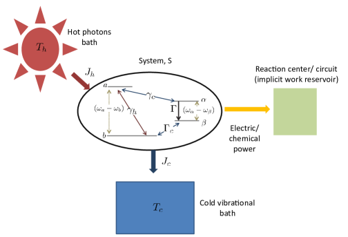
Figure S1: Biological quantum heat engine model from Dorfman et al. (2013).

2) We consider the photocell model proposed in Creatore et al. (2013). It consists of a five level system coupled to a hot bath, a cold bath and to the reaction center/circuit (also termed “the load”). $T_{h(c)}$ is the hot (cold) bath temperature. The decay rates are shown in Figure S2. For the sake of simplicity we assume there is no acceptor-to-donor recombination ($\chi=0$, in the original paper notation). The equations of motion are

$$\dot{\rho}_{\alpha\alpha}=\gamma_{c}\left[\left(1+n_{2c}\right)\rho_{x2x2}-n_{2c}\rho_{\alpha\alpha}\right]-\Gamma\rho_{\alpha\alpha},$$

$$\dot{\rho}_{x2x2}=\gamma_{x}\left[(1+n_{x})\rho_{x1x1}-n_{x}\rho_{x2x2}\right]-\gamma_{c}\left[(1+n_{2c})\rho_{x2x2}-n_{2c}\rho_{\alpha\alpha}\right],$$

$$\dot{\rho}_{bb}=-\left[\gamma_{h}n_{h}+\Gamma_{c}N_{c}\right]\rho_{bb}+\gamma_{h}\left(n_{h}+1\right)\rho_{x1x1}+\Gamma_{c}(N_{c}+1)\rho_{\beta\beta},$$

$$\dot{\rho}_{x1x1}=-\gamma_{x}\left[(1+n_{x})\rho_{x1x1}-n_{x}\rho_{x2x2}\right]-\gamma_{h}\left[(1+n_{h})\rho_{x1x1}-n_{h}\rho_{bb}\right],$$

$$\rho_{x1x1}+\rho_{x2x2}+\rho_{bb}+\rho_{\alpha\alpha}+\rho_{\beta\beta}=1.$$ (S10)

where we have kept the original paper notation. $\rho_{ii}$ is the level population of state $i$ and $n_{i}$ or $N_{i}$ are the relevant i- bath mode population. For details on Eq. S10 derivation, we refer the reader to the original paper. The steady state populations are

$$\frac{\rho_{x2x2}^{ss}}{\rho_{\alpha\alpha}^{ss}}=\frac{\Gamma+\gamma_{c}n_{2c}}{\gamma_{c}\left(1+n_{2c}\right)},$$ (S11)

$$\frac{\rho_{x1x1}^{ss}}{\rho_{x2x2}^{ss}}=\frac{\gamma_{x}n_{x}+\gamma c\left(1+n_{2c}\right)-\gamma_{c}n_{2c}\frac{\gamma_{c}\left(1+n_{2c}\right)}{\Gamma+\gamma_{c}n_{2c}}}{\gamma_{x}\left(1+n_{x}\right)}=\frac{\gamma_{x}n_{x}\left(\Gamma+\gamma_{c}n_{2c}\right)+\gamma c\left(1+n_{2c}\right)\Gamma}{\gamma_{x}\left(1+n_{x}\right)\left(\Gamma+\gamma_{c}n_{2c}\right)},$$ (S12)

$$\frac{\rho_{x1x1}^{ss}}{\rho_{bb}^{ss}}=\frac{\gamma_{h}n_{h}\left[\gamma_{x}n_{x}\left(\Gamma+\gamma_{c}n_{2c}\right)+\gamma_{c}(1+n_{2c})\Gamma\right]}{\gamma_{x}\gamma_{c}\Gamma\left(1+n_{x}\right)\left(1+n_{2c}\right)+\gamma_{h}\left(1+n_{h}\right)\left[\gamma_{x}n_{x}\left(\Gamma+\gamma_{c}n_{2c}\right)+\gamma_{c}(1+n_{2c})\Gamma\right]},$$ (S13)

$$\frac{\rho_{\beta\beta}^{ss}}{\rho_{bb}^{ss}}=e^{-(\omega_{\beta}-\omega_{b})/T_{c}}+\frac{\gamma_{h}n_{h}\gamma_{x}\gamma_{c}\Gamma\left(1+n_{x}\right)\left(1+n_{2c}\right)}{\Gamma_{c}\left(1+N_{c}\right)\left\{\gamma_{x}\gamma_{c}\Gamma\left(1+n_{x}\right)\left(1+n_{2c}\right)+\gamma_{h}\left(1+n_{h}\right)\left[\gamma_{x}n_{x}\left(\Gamma+\gamma_{c}n_{2c}\right)+\gamma_{c}\left(1+n_{2c}\right)\Gamma\right]\right\}}.$$ (S14)

Using Eq. S6 the steady state heat currents are obtained,

$$J_{h}=\left(\omega_{x1}-\omega_{b}\right)\left(1+\bar{n}_{h}\right)\gamma_{h}\rho_{bb}^{ss}\left(e^{-(\omega_{x1}-\omega_{b})/T_{h}}-\frac{\rho_{x1x1}^{ss}}{\rho_{bb}^{ss}}\right)=$$

$$\left(\omega_{x1}-\omega_{b}\right)\frac{\rho_{bb}^{ss}\gamma_{h}n_{h}\gamma_{x}\gamma_{c}\Gamma\left(1+n_{x}\right)\left(1+n_{2c}\right)}{\gamma_{x}\gamma_{c}\Gamma\left(1+n_{x}\right)\left(1+n_{2c}\right)+\gamma_{h}\left(1+n_{h}\right)\left[\gamma_{x}n_{x}\left(\Gamma+\gamma_{c}n_{2c}\right)+\gamma_{c}\left(1+n_{2c}\right)\Gamma\right]},$$ (S15)

$$J_{c}=\left(\omega_{x1}-\omega_{x2}\right)\left(1+\bar{n}_{x}\right)\gamma_{x}\rho_{x2x2}^{ss}\left(e^{-(\omega_{x1}-\omega_{x2})/T_{c}}-\frac{\rho_{x1x1}^{ss}}{\rho_{x2x2}^{ss}}\right)+$$

$$\left(\omega_{x2}-\omega_{\alpha}\right)\left(1+\bar{n}_{2c}\right)\gamma_{c}\rho_{\alpha\alpha}^{ss}\left(e^{-(\omega_{x2}-\omega_{\alpha})/T_{c}}-\frac{\rho_{x2x2}^{ss}}{\rho_{\alpha\alpha}^{ss}}\right)+\left(\omega_{\beta}-\omega_{b}\right)\left(1+\bar{N}_{c}\right)\Gamma_{c}\rho_{bb}^{ss}\left(e^{-(\omega_{\beta}-\omega_{b})/T_{c}}-\frac{\rho_{\beta\beta}^{ss}}{\rho_{bb}^{ss}}\right)=$$

$$-\frac{\rho_{bb}^{ss}\gamma_{h}n_{h}\gamma_{x}\gamma_{c}\Gamma\left(1+n_{x}\right)\left(1+n_{2c}\right)}{\gamma_{x}\gamma_{c}\Gamma\left(1+n_{x}\right)\left(1+n_{2c}\right)+\gamma_{h}\left(1+n_{h}\right)\left[\gamma_{x}n_{x}\left(\Gamma+\gamma_{c}n_{2c}\right)+\gamma_{c}\left(1+n_{2c}\right)\Gamma\right]}\left(\omega_{x1}+\omega_{\beta}-\omega_{\alpha}-\omega_{b}\right),$$ (S16)

$$\frac{-J_{c}}{J_{h}}=\frac{\omega_{x1}+\omega_{\beta}-\omega_{\alpha}-\omega_{b}}{\omega_{x1}-\omega_{b}}=1+\frac{\omega_{\beta}-\omega_{\alpha}}{\omega_{x1}-\omega_{b}},$$ (S17)

where $\omega_{x1}-\omega_{b}$ ($\omega_{\alpha}-\omega_{\beta}$) is the energy of the absorbed (emitted) quanta from the hot bath (to the RC/circuit), therefore equivalent to $\omega_{abs}(\omega_{rc})$. Using this paper notation,

$$J_{h}\rightarrow J_{abs},$$

$$J_{c}\rightarrow J_{loss},$$

$$\omega_{\beta}-\omega_{\alpha}\rightarrow-\omega_{rc},$$

$$\omega_{x1}-\omega_{b}\rightarrow\omega_{abs},$$

$$T_{h}\rightarrow T_{abs},$$

$$T_{c}\rightarrow T_{loss},$$

we obtain Eq. 3 in the main text.

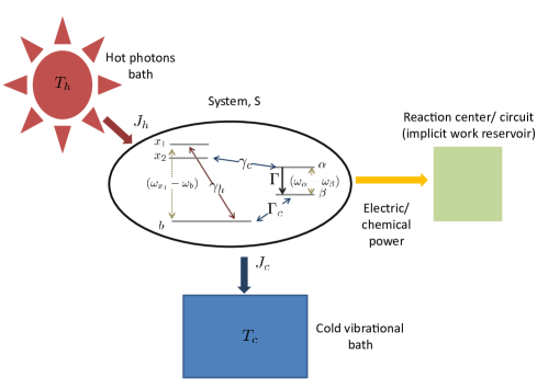
Figure S2: Photocell model proposed in Creatore et al. (2013).

I.2 FMO models

We start by considering the model proposed on Adolphs and Renger (2006) for the Fenna-Mathews-Olson complex of a Prosthecochloris aestuarii. Its dynamics is governed by the following Hamiltonian,

$$H_{FMO}+H_{FMO-vib}+H_{vib},$$ (S18)

where $H_{vib}$ is the free Hamiltonian for the vibrational degrees of freedom of the pigments and proteins, which we assume to be at equilibrium at a temperature $T_{loss}=300K.$ $H_{FMO}$ is the exciton Hamiltonian,

$$H_{FMO}=\sum_{m\in FMO}E_{m}|m\rangle\langle m|+\sum_{m\neq n\in FMO}V_{mn}|m\rangle\langle n|,$$ (S19)

where $|m\rangle$ is the excited state of the $m$ site, and the sum is over all the FMO sites. $H_{FMO-vib}$ represents the interaction between the excitons and the vibrations,

$$H_{FMO-vib}=\sum_{m\in FMO,\xi}k_{\xi}^{m}|m\rangle\langle m|\otimes Q_{\xi},$$ (S20)

where $Q_{\xi}$ operates on the vibration degrees of freedom. All the parameters for this Hamiltonian can be found on Adolphs and Renger (2006).

In order to thermodynamically analyze the FMO we complement the above model with the following elements:

1) Energy transmission to the reaction center;

2) Absorption of thermal radiation by the antenna and its transmission to the reaction center (RC), as well as the possibility for the FMO sites to interact with the thermal radiation.

I.2.1 Transmission of energy to the reaction center

The transmission of energy to the reaction center is typically modeled Mohseni et al. (2008); Rebentrost et al. (2009); Plenio and Huelga (2008); Killoran et al. (2014); Alharbi and Kais (2015); Cao and Silbey (2009); Caruso et al. (2009) as an irreversible decay term from the FMO site 3 to 8,

$$H_{Dec}=\sqrt{\Gamma_{3,8}}|8\rangle\langle 3|.$$ (S21)

We use a typical value for this rate, $\Gamma_{3,8}=62.8/1.88\,cm^{-1}$Mohseni et al. (2008); Rebentrost et al. (2009); Plenio and Huelga (2008); Caruso et al. (2009).

I.2.2 Antenna and thermal radiation

The antenna is composed of around 10,000 absorbing pigments Valleau et al. (2014). As a simple model we consider the collective effect of these pigments as an effective monochromatic antenna of frequency $\omega_{ant}=13333cm^{-1}$, with an effective molecular transition dipole moment $\mu_{ant}=\sqrt{N}\mu_{ant,ind},$ where $N$ is the number of absorbing pigments and $\mu_{ant,ind}\sim 5$ Debye, a typical value for a molecular transition dipole moment.

Light absorption is governed by the antenna-radiation coupling Hamiltonian,

$$H_{ant-rad}=\mu_{ant}|ant\rangle\langle 0|\otimes B_{abs}+h.c.,$$ (S22)

where $B_{abs}$ is an operator on the thermal radiation bath, $|ant\rangle$ is the antenna excited state and $|0\rangle$ is the ground state. The FMO sites may also interact with the thermal radiation through the Hamiltonian,

$$H_{FMO-rad}=\sum_{m}\mu_{FMO}|m\rangle\langle 0|\otimes B_{abs}+h.c.,$$ (S23)

where $\mu_{FMO}=5.44$ Debye Adolphs and Renger (2006).

The transmission of the excitation from the antenna to the FMO is assisted by the vibration degrees of freedom described by the Hamiltonian,

$$H_{ant-FMO}=\sum_{\xi,m\in FMO}\sqrt{\Gamma_{ant-FMO}}|m\rangle\langle ant|\otimes Q_{\xi}+h.c$$ (S24)

and we assume that $\Gamma_{ant-FMO}=\Gamma_{3,8}/10$.

Even though at the sun surface the thermal radiation emitted by the sun is at equilibrium at the sun temperature, due to geometric considerations, only a small fraction of those photons reaches the Earth. This is quantified by a geometric factor $\lambda=2*10^{-5}$ equal to the angle subtended by the Sun seen from the Earth. If $n_{T_{S}}\left[\omega\right]=(e^{\omega/T_{S}}-1)^{-1}$ photons of frequency $\omega,$ are emitted from the sun at temperature $T_{s}$, only $\lambda n_{T_{s}}$ reach the Earth. This radiation is no longer a thermal bath at the sun temperature, but rather is a non-equilibrium bath at an effective temperature Alicki and Gelbwaser-Klimovsky (2015); Landsberg and Tonge (1980),

$$e^{-\omega_{ant}/T_{abs}}=\frac{\lambda n_{T}\left[\omega_{ant}\right]}{\lambda n_{T}\left[\omega_{ant}\right]+1}\rightarrow T_{abs}\sim 1356K.$$ (S25)

The dilution of the photon numbers turns the effective temperature, $T_{abs}$, frequency dependent. Nevertheless, the frequency variation between the antenna and the FMO site is small, therefore we assume the same $T_{abs}$ for the antenna and the FMO sites.

Dynamic equations

Collecting everything together, we can write the total Hamiltonian,

$$H_{Tot}=H_{FMO}+H_{FMO-vib}+H_{vib}+H_{ant}+H_{ant-FMO}+H_{ant-rad}+H_{FMO-rad}+H_{rad}+H_{Dec},$$ (S26)

where $H_{ant(rad)}$ is the antenna (radiation) free Hamiltonian.

Using the standard Born-Markov approximation, the Lindblad equation Lindblad (1976) for the FMO is numerically found, enabling the calculation of the heat currents defined by Eq. S6. $J_{abs}$ ($J_{loss}$) corresponds to the heat current between the radiation (vibration) bath and the FMO.

II Simple models for the RC/circuit

We consider a three level system (3LS), S, coupled to the reaction center (RC) or electric circuit. The later is a reservoir of independent quinones/sites, each of them represented by a single two level system (TLS). Its ground state represents an empty quinone/site and the excited state corresponds to a full quinone/site. Besides, the 3LS is coupled to a photon (hot) bath and a vibrational (cold) bath (see Figure 3 in the main text). The total Hamiltonian is

$$H_{S}+H_{B}+H_{SB},$$ (S27)

where $H_{B}=H_{photons}+H_{phonons}$ is the baths free Hamiltonian. The S-baths coupling Hamiltonian is given by

$$H_{SB}=S\otimes\left(B_{h}+B_{c}\right)=\sum_{\lambda}g_{h,\lambda}\left(|2\rangle\langle 0|a_{\lambda}+|0\rangle\langle 2|a_{\lambda}^{\dagger}\right)+\sum_{\lambda}g_{c,\lambda}\left(|2\rangle\langle 1|b_{\lambda}+|1\rangle\langle 2|b_{\lambda}^{\dagger}\right),$$ (S28)

where $a_{\lambda},$$a_{\lambda}^{\dagger}$ ($b_{\lambda},$ $b{}_{\lambda}^{\dagger}$) are the annihilation and creation operator of photons (phonons) modes. The S + RC/circuit Hamiltonian is

$$H_{S}=H_{0}+H_{trans},$$ (S29)

$$H_{0}=\omega_{abs}|2\rangle\langle 2|+\frac{\omega_{rc}}{2}\left(|1\rangle\langle 1|-|0\rangle\langle 0|\right),$$ (S30)

where $H_{0}$ is the 3LS free Hamiltonian and $H_{trans}$ describes the energy transfer to the RC/circuit. We compare between two possible schemes: i) A decay transfer described by a non-hermitian $H_{trans}$; ii) a Hamiltonian transfer, represented by a hermitic $H_{trans}$.

II.1 Decay transfer

The decay transfer is described by the following non-hermitian term,

$$H_{tranf}^{Dec}=\sqrt{\Gamma}|0\rangle\langle 1|.$$ (S31)

As a first step we transform the S-bath interaction and the transfer Hamiltonian to the interaction picture

$$H_{SB}\rightarrow e^{iH_{0}t}H_{SB}e^{-iH_{0}t},\quad H_{tranf}^{Dec}\rightarrow e^{iH_{0}t}H_{tranf}^{Dec}e^{-iH_{0}t}.$$ (S32)

$H_{tranf}^{Dec}$ is a fictitious Hamiltonian due to its lack of hermiticity, therefore can not form part of the rotation, $e^{iH_{0}t}$ , which has to be unitary. Besides, we derive the reduced dynamics only for S. The operators in the interaction picture are:

$$|2\rangle\langle 0|\left[t\right]=e^{it\left(\omega_{abs}+\frac{\omega_{rc}}{2}\right)}|2\rangle\langle 0|,$$ (S33)

$$|2\rangle\langle 1|\left[t\right]=e^{it\left(\omega_{abs}-\frac{\omega_{rc}}{2}\right)}|2\rangle\langle 1|,$$ (S34)

$$|0\rangle\langle 1|\left[t\right]=e^{-it\omega_{rec}}|0\rangle\langle 1|.$$ (S35)

Using the standard Born-Markov approximation, the Lindblad equation Lindblad (1976) for S is obtained

$$\dot{\rho}_{22}=$$

$$-\left\{\Gamma_{h}\left(1+n_{h}\left[\omega_{abs}+\frac{\omega_{rc}}{2}\right]\right)+\Gamma_{c}\left(1+n_{c}\left[\omega_{abs}-\frac{\omega_{rc}}{2}\right]\right)\right\}\rho_{22}+\Gamma_{h}n_{h}\left[\omega_{abs}+\frac{\omega_{rc}}{2}\right]\rho_{00}+\Gamma_{c}n_{c}\left[\omega_{abs}-\frac{\omega_{rc}}{2}\right]\rho_{11},$$ (S36)

$$\dot{\rho}_{11}=-\left\{\Gamma+\Gamma_{c}n_{c}\left[\omega_{abs}-\frac{\omega_{rc}}{2}\right]\right\}\rho_{11}+\Gamma_{c}\left(1+n_{c}\left[\omega_{abs}-\frac{\omega_{rc}}{2}\right]\right)\rho_{22},$$ (S37)

$$\dot{\rho}_{00}=-\Gamma_{h}n_{h}\left[\omega_{abs}+\frac{\omega_{rc}}{2}\right]\rho_{00}+\Gamma_{h}\left(1+n_{h}\left[\omega_{abs}+\frac{\omega_{rc}}{2}\right]\right)\rho_{22}+\Gamma\rho_{11},$$ (S38)

where $\Gamma_{i}$ and $n_{i}\left[\omega\right]$ are the decay rate and $\omega$-mode population of the i-bath. The steady state is

$$\frac{\rho_{22}^{ss}}{\rho_{11}^{ss}}=\frac{\Gamma+\Gamma_{c}n_{c}\left[\omega_{abs}-\frac{\omega_{rc}}{2}\right]}{\Gamma_{c}\left(1+n_{c}\left[\omega_{abs}-\frac{\omega_{rc}}{2}\right]\right)},$$ (S39)

$$\frac{\rho_{22}^{ss}}{\rho_{00}^{ss}}=e^{-\left(\omega_{abs}+\frac{\omega_{rc}}{2}\right)/T_{abs}}-\frac{\Gamma\rho_{11}^{ss}}{\Gamma_{h}\left(1+n_{h}\left[\omega_{abs}+\frac{\omega_{rc}}{2}\right]\right)\rho_{00}^{ss}},$$ (S40)

$$\frac{\rho_{11}^{ss}}{\rho_{00}^{ss}}=\frac{\Gamma_{h}n_{h}\left[\omega_{abs}+\frac{\omega_{rc}}{2}\right]\Gamma_{c}\left(1+n_{c}\left[\omega_{abs}-\frac{\omega_{rc}}{2}\right]\right)}{\Gamma_{c}n_{c}\left[\omega_{abs}-\frac{\omega_{rc}}{2}\right]\Gamma_{h}\left(1+n_{h}\left[\omega_{abs}+\frac{\omega_{rc}}{2}\right]\right)+\Gamma\left\{\Gamma_{h}\left(1+n_{h}\left[\omega_{abs}+\frac{\omega_{rc}}{2}\right]\right)+\Gamma_{c}\left(1+n_{c}\left[\omega_{abs}-\frac{\omega_{rc}}{2}\right]\right)\right\}},$$ (S41)

$$\rho_{11}^{ss}=\frac{1}{1+\frac{\rho_{00}^{ss}}{\rho_{11}^{ss}}+\frac{\rho_{22}^{ss}}{\rho_{11}^{ss}}}=\frac{1}{1+2e^{\left(\omega_{abs}+\frac{\omega_{rc}}{2}\right)/T_{abs}}}.$$ (S42)

In the last equality, we assume for simplicity that all the zero temperature decay rates are equal to the RC decay rate, $\Gamma_{c}=\Gamma_{h}=\Gamma$. Using Eq. S6 the heat currents at steady state are obtained,

$$J_{abs}^{Dec}\equiv J_{h}^{Dec}=\left(\omega_{abs}+\frac{\omega_{rc}}{2}\right)\rho_{00}^{ss}\Gamma_{h}\left(1+n_{h}\left[\omega_{abs}+\frac{\omega_{rc}}{2}\right]\right)\left[e^{-\left(\omega_{abs}+\frac{\omega_{rc}}{2}\right)/T_{abs}}-\frac{\rho_{22}^{ss}}{\rho_{00}^{ss}}\right]=\left(\omega_{abs}+\frac{\omega_{rc}}{2}\right)\Gamma\rho_{11}^{ss},$$ (S43)

$$J_{loss}^{Dec}\equiv J_{c}^{Dec}=\left(\omega_{abs}-\frac{\omega_{rc}}{2}\right)\rho_{11}^{ss}\Gamma_{c}\left(1+n_{c}\left[\omega_{abs}-\frac{\omega_{rc}}{2}\right]\right)\left[e^{-\left(\omega_{abs}-\frac{\omega_{rc}}{2}\right)/T_{loss}}-\frac{\rho_{22}^{ss}}{\rho_{11}^{ss}}\right]=-\left(\omega_{abs}-\frac{\omega_{rc}}{2}\right)\Gamma\rho_{11}^{ss}$$ (S44)

and by energy conservation the power is

$$P^{Dec}=-J_{abs}^{Dec}-J_{loss}^{Dec}=-\omega_{rc}\Gamma\rho_{11}^{ss}<0.$$ (S45)

This model predicts that power is extracted independently of the baths temperatures, in contradiction with the second law of thermodynamics which forbids power extraction in the case of a single temperature, $T_{loss}=T_{abs}$. As shown in Figure 4 of the main text, also for $T_{loss}\neq T_{abs}$, $P^{Dec}$ diverges from the extracted power predicted by a thermodynamically consistent model.

II.2 Hamiltonian transfer

Here we explicitly consider the RC/circuit and its coupling to S, by considering $H_{trans}$ as an hermitic Hamiltonian. The RC/circuit is composed of identical and independent two level systems (TLS). The S + RC/circuit Hamiltonian is:

$$H_{S}=\omega_{abs}|2\rangle\langle 2|+\frac{\omega_{rc}}{2}\left(|1\rangle\langle 1|-|0\rangle\langle 0|\right)+\sum_{k}^{j}\sqrt{\frac{\Gamma}{2j}}\left(\sigma_{-}^{k}|1\rangle\langle 0|+\sigma_{+}^{k}|0\rangle\langle 1|\right)+\omega_{rc}\sum_{k}\sigma_{z}^{k},$$ (S46)

where $j$ is the number of TLSs.

In order to find the energy that is being transferred to the RC/circuit, we start by diagonalizing the S + RC circuit. This is achieved by first applying the Holstein-Primakoff transformation Holstein and Primakoff (1940), that consist on the introduction of the following collective operators:

$$\sum_{k}\sigma_{-}^{k}=\left(\sqrt{2j-c^{\dagger}c}\right)c,$$ (S47)

$$\sum_{k}\sigma_{+}^{k}=c^{\dagger}\left(\sqrt{2j-c^{\dagger}c}\right),$$ (S48)

$$\sum_{k}\sigma_{z}^{k}=c^{\dagger}c-j.$$ (S49)

The new Hamiltonian is

$$H_{S}=\omega_{abs}|2\rangle\langle 2|+\frac{\omega_{rc}}{2}\left(|1\rangle\langle 1|-|0\rangle\langle 0|\right)+\sqrt{\frac{\Gamma}{2j}}\left[\left(\sqrt{2j-c^{\dagger}c}\right)c|1\rangle\langle 0|+c^{\dagger}\left(\sqrt{2j-c^{\dagger}c}\right)|0\rangle\langle 1|\right]+\omega_{rc}\left(c^{\dagger}c-j\right).$$ (S50)

At this point, the modes are displaced, $c\rightarrow c-\sqrt{\epsilon}$,

$$H_{S}=\omega_{abs}|2\rangle\langle 2|+\frac{\omega_{rc}}{2}\left(|1\rangle\langle 1|-|0\rangle\langle 0|\right)+\sqrt{\frac{\Gamma k\eta}{2j}}\left(c|1\rangle\langle 0|+c^{\dagger}|0\rangle\langle 1|\right)-\sqrt{\frac{\Gamma k\eta\epsilon}{2j}}\left(|1\rangle\langle 0|+|0\rangle\langle 1|\right)+$$

$$\omega_{rc}\left(c^{\dagger}c-\sqrt{\epsilon}(c+c^{\dagger})+\epsilon-j\right),$$ (S51)

where $k=2j-\epsilon$ and $\eta=1-\frac{c^{\dagger}c-\sqrt{\epsilon}(c^{\dagger}+c)}{k}$. We assume that the number of TLSs is large, $\frac{c^{\dagger}c-\sqrt{\epsilon}(c^{\dagger}+c)}{k}\ll 1$. The physical interpretation of this approximation is clarified below. Under this assumptions, we expand $\sqrt{\eta}\approx 1-\frac{c^{\dagger}c-\sqrt{\epsilon}(c^{\dagger}+c)}{2k}-\frac{\epsilon(c^{\dagger}+c)^{2}}{8k^{2}}$ and keep terms up to order $\frac{1}{\sqrt{j}},$

$$H_{S}=\omega_{abs}|2\rangle\langle 2|+\frac{\omega_{rc}}{2}\left(|1\rangle\langle 1|-|0\rangle\langle 0|\right)-\sqrt{\frac{\Gamma k\epsilon}{2j}}\left(|1\rangle\langle 0|+|0\rangle\langle 1|\right)+\sqrt{\frac{\Gamma k}{2j}}\left(c|1\rangle\langle 0|+c^{\dagger}|0\rangle\langle 1|\right)-$$

$$\frac{\epsilon}{2}\sqrt{\frac{\Gamma}{2jk}}\left(c^{\dagger}+c\right)\left(|1\rangle\langle 0|+|0\rangle\langle 1|\right)+\omega_{rc}\left(c^{\dagger}c-\sqrt{\epsilon}\left(c+c^{\dagger}\right)+\epsilon-j\right).$$ (S52)

Setting $\epsilon=0$, the Hamiltonian is simplified to

$$H_{S}=\omega_{abs}|2\rangle\langle 2|+\frac{\omega_{rc}}{2}\left(|1\rangle\langle 1|-|0\rangle\langle 0|\right)+\sqrt{\Gamma}\left(c|1\rangle\langle 0|+c^{\dagger}|0\rangle\langle 1|\right)+\omega_{rc}\left(c^{\dagger}c-j\right)$$ (S53)

and the approximation to $\frac{c^{\dagger}c}{2j}\ll 1$. Therefore, we are just assuming that the total number of excitations in the RC/circuit is very small compared to the number of quinones/sites, so energy may always be transferred to the RC/circuit. From Eq. S53, we derive Eq. 9 in the main text,

$$H_{trasns}^{emi}=\sqrt{\Gamma}\left(c|1\rangle\langle 0|+c^{\dagger}|0\rangle\langle 1|\right)+\omega_{rc}\left(c^{\dagger}c-j\right).$$ (S54)

Next we diagonalize Eq. S53. The Hamiltonian eigenvectors are

$$|+,n\rangle=\frac{1}{\sqrt{2}}\left(|1,n\rangle+|0,n+1\rangle\right),$$ (S55)

$$|-,n\rangle=\frac{1}{\sqrt{2}}\left(|0,n+1\rangle-|1,n\rangle\right),$$ (S56)

$$E_{\pm}=\omega_{rc}\left(n+\frac{1}{2}\right)\pm\frac{\Omega_{n}}{2}-j\omega_{rc},$$ (S57)

$$H_{S}=\omega_{abs}|2\rangle\langle 2|+\omega_{rc}\left(\tilde{c}^{\dagger}\tilde{c}+\frac{1}{2}\sum_{n}\left(\left|+,n\right\rangle\langle+,n|+|-,n\rangle\langle-,n|\right)-j\right)+\frac{\Omega_{n}}{2}\tilde{\sigma}_{z},$$ (S58)

where $\tilde{c}^{\dagger}(\tilde{c})$ is the creation (annihilation) operator in the new basis and $\Omega_{n}=2\sqrt{\Gamma(n+1)}$. The inverse transformations are

$$|1,n\rangle=\frac{1}{\sqrt{2}}\left(|+,n\rangle-|-,n\rangle\right),$$ (S59)

$$|0,n+1\rangle=\frac{1}{\sqrt{2}}\left(|+,n\rangle+|-,n\rangle\right).$$ (S60)

Rewriting the S-bath Hamiltonian, Eq. S28 , in the new basis,

$$|2\rangle\langle 0|=\sum_{n}\frac{1}{\sqrt{2}}\left(|2,n+1\rangle\langle+,n|+|2,n+1\rangle\langle-,n|\right),$$ (S61)

$$|2\rangle\langle 1|=\sum_{n}\frac{1}{\sqrt{2}}\left(|2,n\rangle\langle+,n|-|2,n\rangle\langle-,n|\right),$$ (S62)

and transforming to the interaction picture,

$$H_{SB}\rightarrow e^{iH_{S}t}H_{SB}e^{-iH_{S}t},$$ (S63)

$$|2\rangle\langle 0|\left[t\right]=\sum_{n}\frac{1}{\sqrt{2}}\left(e^{it\left(\omega_{abs}+\frac{\omega_{rc}}{2}-\frac{\Omega_{n}}{2}\right)}|2,n+1\rangle\langle+,n|+e^{it\left(\omega_{abs}+\frac{\omega_{rc}}{2}+\frac{\Omega_{n}}{2}\right)}|2,n+1\rangle\langle-,n|\right),$$ (S64)

$$|2\rangle\langle 1|\left[t\right]=\sum_{n}\frac{1}{\sqrt{2}}\left(e^{it\left(\omega_{abs}-\frac{\omega_{rc}}{2}-\frac{\Omega_{n}}{2}\right)}|2,n\rangle\langle+,n|-e^{it\left(\omega_{abs}-\frac{\omega_{rc}}{2}+\frac{\Omega_{n}}{2}\right)}|2,n\rangle\langle-,n|\right).$$ (S65)

In contrast to the decay transfer scheme (Eq. S32), here $H_{trans}^{Ham}$ is hermitian and we derive the reduced dynamics for the S + RC/circuit. Therefore $H_{trans}^{Ham}$ is included in the rotation, $e^{iH_{S}t}$.

Using the standard Born-Markov approximation, the Lindblad equation Lindblad (1976) for S + RC/circuit is obtained, and from it the evolution equations are derived,

$$\dot{\rho}_{+,n}=\frac{1}{2}\left\{-\Gamma_{h}n_{h}\left[\omega_{abs}+\frac{\omega_{rc}-\Omega_{n}}{2}\right]\rho_{+,n}+\Gamma_{h}\left(1+n_{h}\left[\omega_{abs}+\frac{\omega_{rc}-\Omega_{n}}{2}\right]\right)\rho_{2,n+1}\right\}+$$

$$\frac{1}{2}\left\{-\Gamma_{c}n_{c}\left[\omega_{abs}-\frac{\omega_{rc}+\Omega_{n}}{2}\right]\rho_{+,n}+\Gamma_{c}\left(1+n_{c}\left[\omega_{abs}-\frac{\omega_{rc}+\Omega_{n}}{2}\right]\right)\rho_{2,n}\right\},$$

$$\dot{\rho}_{-,n}=\frac{1}{2}\left\{-\Gamma_{h}n_{h}\left[\omega_{abs}+\frac{\omega_{rc}+\Omega_{n}}{2}\right]\rho_{-,n}+\Gamma_{h}\left(1+n_{h}\left[\omega_{abs}+\frac{\omega_{rc}+\Omega_{n}}{2}\right]\right)\rho_{2,n+1}\right\}+$$

$$\frac{1}{2}\left\{-\Gamma_{c}n_{c}\left[\omega_{abs}-\frac{\omega_{rc}-\Omega_{n}}{2}\right]\rho_{-,n}+\Gamma_{c}\left(1+n_{c}\left[\omega_{abs}-\frac{\omega_{rc}-\Omega_{n}}{2}\right]\right)\rho_{2,n}\right\},$$

$$\dot{\rho}_{2,n}=\frac{1}{2}\left\{\Gamma_{h}n_{h}\left[\omega_{abs}+\frac{\omega_{rc}-\Omega_{n-1}}{2}\right]\rho_{+,n-1}-\Gamma_{h}\left(1+n_{h}\left[\omega_{abs}+\frac{\omega_{rc}-\Omega_{n-1}}{2}\right]\right)\rho_{2,n}\right\}+$$

$$\frac{1}{2}\left\{\Gamma_{h}n_{h}\left[\omega_{abs}+\frac{\omega_{rc}+\Omega_{n-1}}{2}\right]\rho_{-,n-1}-\Gamma_{h}\left(1+n_{h}\left[\omega_{abs}+\frac{\omega_{rc}+\Omega_{n-1}}{2}\right]\right)\rho_{2,n}\right\}+$$

$$\frac{1}{2}\left\{\Gamma_{c}n_{c}\left[\omega_{abs}-\frac{\omega_{rc}+\Omega_{n}}{2}\right]\rho_{+,n}-\Gamma_{c}\left(1+n_{c}\left[\omega_{abs}-\frac{\omega_{rc}+\Omega_{n}}{2}\right]\right)\rho_{2,n}\right\}+$$ (S66)

$$\frac{1}{2}\left\{\Gamma_{c}n_{c}\left[\omega_{abs}-\frac{\omega_{rc}-\Omega_{n}}{2}\right]\rho_{-,n}-\Gamma_{c}\left(1+n_{c}\left[\omega_{abs}-\frac{\omega_{rc}-\Omega_{n}}{2}\right]\right)\rho_{2,n}\right\},$$

where $\rho_{i}$ is the population of the combined state $i$ (S + RC/circuit), $\Gamma_{i}$ and $n_{i}\left[\omega\right]$ are the decay rate and $\omega$-mode population of the i-bath. The equations for the off-diagonal terms are decoupled from the populations and we assume them to be zero. If the coupling between the 3LS and the RC/circuit is weak, $\omega_{rc}\gg\Omega_{n}$, it can be assumed that they are in a product state. Moreover, if the coupling spectrum is approximately flat in frequency windows of size $\Omega_{n}-\Omega_{n-1}$, the 3LS steady state is

$$\frac{\rho_{2}^{ss}}{\rho_{+}^{ss}}=\frac{\rho_{2}^{ss}}{\rho_{-}^{ss}}=\frac{\Gamma_{h}n_{h}\left[\omega_{abs}+\frac{\omega_{rc}}{2}\right]+\Gamma_{c}n_{c}\left[\omega_{abs}-\frac{\omega_{rc}}{2}\right]}{\Gamma_{h}\left(1+n_{h}\left[\omega_{abs}+\frac{\omega_{rc}}{2}\right]\right)+\Gamma_{c}\left(1+n_{c}\left[\omega_{abs}-\frac{\omega_{rc}}{2}\right]\right)}=\frac{n_{h}\left[\omega_{abs}+\frac{\omega_{rc}}{2}\right]+n_{c}\left[\omega_{abs}-\frac{\omega_{rc}}{2}\right]}{2+n_{h}\left[\omega_{abs}+\frac{\omega_{rc}}{2}\right]+n_{c}\left[\omega_{abs}-\frac{\omega_{rc}}{2}\right]},$$ (S67)

$$\rho_{+}^{ss}=\frac{2+n_{h}\left[\omega_{abs}+\frac{\omega_{rc}}{2}\right]+n_{c}\left[\omega_{abs}-\frac{\omega_{rc}}{2}\right]}{4+3n_{h}\left[\omega_{abs}+\frac{\omega_{rc}}{2}\right]+3n_{c}\left[\omega_{abs}-\frac{\omega_{rc}}{2}\right]}.$$ (S68)

For the sake of simplicity we have assumed in the last equality that the zero temperature decay rates of both baths are the same as the RC/circuit coupling strength, $\Gamma_{h}=\Gamma_{c}=\Gamma$. From Eqs. S66 an evolution equation for the RC/circuit can be written,

$$\dot{\rho}_{n}=\dot{\rho}_{+,n}+\dot{\rho}_{-,n}+\dot{\rho}_{2,n}=r\rho_{n+1}+s\rho_{n-1}-(r+s)\rho_{n},$$ (S69)

which is a “birth-death process” Van Kampen (1992), where $s(r)$ is the birth (death) rate,

$$s=\frac{1}{2}\Gamma_{h}n_{h}\left[\omega_{abs}+\frac{\omega_{rc}}{2}\right]\left(\rho_{+}+\rho_{-}\right),\quad r=\Gamma_{h}\left(1+n_{h}\left[\omega_{abs}+\frac{\omega_{rc}}{2}\right]\right)\rho_{2}.$$ (S70)

The energy change of the RC/circuit evolves as

$$\omega_{rc}\langle\dot{n}\rangle=\left(s-r\right)\omega_{rc},$$ (S71)

which is equal to $-P^{Ham}$ (the used sign convention can be found below Eq. 1 in the main text).

Thus, $s>r$ is required in order to increase the RC/circuit energy. At the 3LS steady state, this implies,

$$s-r=\frac{\Gamma\left(1+n_{c}\left[\omega_{abs}-\frac{\omega_{rc}}{2}\right]\right)\left(1+n_{h}\left[\omega_{abs}+\frac{\omega_{rc}}{2}\right]\right)}{4+3n_{h}\left[\omega_{abs}+\frac{\omega_{rc}}{2}\right]+3n_{c}\left[\omega_{abs}-\frac{\omega_{rc}}{2}\right]}\left(e^{-\left(\omega_{abs}+\frac{\omega_{rc}}{2}\right)/T_{abs}}-e^{-\left(\omega_{abs}-\frac{\omega_{rc}}{2}\right)/T_{loss}}\right)=$$

$$K_{1}\left(e^{-\left(\omega_{abs}+\frac{\omega_{rc}}{2}\right)/T_{abs}}-e^{\left(\omega_{abs}-\frac{\omega_{rc}}{2}\right)/T_{loss}}\right)>0,$$ (S72)

where $K_{1}=\frac{\Gamma\left(1+n_{c}\left[\omega_{abs}-\frac{\omega_{rc}}{2}\right]\right)\left(1+n_{h}\left[\omega_{abs}+\frac{\omega_{rc}}{2}\right]\right)}{4+3n_{h}\left[\omega_{abs}+\frac{\omega_{rc}}{2}\right]+3n_{c}\left[\omega_{abs}-\frac{\omega_{rc}}{2}\right]}>0$ and the energy gain condition is

$$\frac{T_{loss}}{T_{abs}}<\frac{\omega_{abs}-\frac{\omega_{rc}}{2}}{\omega_{abs}+\frac{\omega_{rc}}{2}}=\frac{2\omega_{abs}-\omega_{rc}}{2\omega_{abs}+\omega_{rc}}.$$ (S73)

Using Eq. S6 the heat currents at steady state are obtained,

$$J_{abs}^{Ham}\equiv J_{h}^{Ham}=\left(\omega_{abs}+\frac{\omega_{rc}}{2}\right)(s-r),$$ (S74)

$$J_{loss}^{Ham}\equiv J_{c}^{Ham}=-\left(\omega_{abs}-\frac{\omega_{rc}}{2}\right)(s-r).$$ (S75)

References

• Blankenship (2013) R. E. Blankenship, Molecular mechanisms of photosynthesis (John Wiley & Sons, 2013).
• Nelson (2003) J. Nelson, The physics of solar cells, vol. 1 (World Scientific, 2003).
• Würfel and Würfel (2009) P. Würfel and U. Würfel, Physics of solar cells: from basic principles to advanced concepts (John Wiley & Sons, 2009).
• Blankenship et al. (2011) R. E. Blankenship, D. M. Tiede, J. Barber, G. W. Brudvig, G. Fleming, M. Ghirardi, M. Gunner, W. Junge, D. M. Kramer, A. Melis, et al., science 332, 805 (2011).
• Alicki et al. (2016) R. Alicki, D. Gelbwaser-Klimovsky, and K. Szczygielski, Journal of Physics A: Mathematical and Theoretical 49, 015002 (2016), URL http://stacks.iop.org/1751-8121/49/i=1/a=015002.
• Einax and Nitzan (2014) M. Einax and A. Nitzan, The Journal of Physical Chemistry C 118, 27226 (2014).
• Kondepudi and Prigogine (2014) D. Kondepudi and I. Prigogine, Modern thermodynamics: from heat engines to dissipative structures (John Wiley & Sons, 2014).
• Gelbwaser-Klimovsky et al. (2015) D. Gelbwaser-Klimovsky, W. Niedenzu, and G. Kurizki, Advances In Atomic, Molecular, and Optical Physics 64, 329 (2015).
• Shockley and Queisser (1961) W. Shockley and H. J. Queisser, Journal of applied physics 32, 510 (1961).
• Landsberg and Tonge (1980) P. Landsberg and G. Tonge, Journal of Applied Physics 51, R1 (1980).
• Knox and Parson (2007) R. S. Knox and W. W. Parson, Biochimica et Biophysica Acta (BBA)-Bioenergetics 1767, 1189 (2007).
• Knox (1969) R. S. Knox, Biophysical journal 9, 1351 (1969).
• Parson (1978) W. W. Parson, Photochemistry and photobiology 28, 389 (1978).
• Ross and Calvin (1967) R. T. Ross and M. Calvin, Biophysical journal 7, 595 (1967).
• Alicki and Gelbwaser-Klimovsky (2015) R. Alicki and D. Gelbwaser-Klimovsky, New Journal of Physics 17, 115012 (2015).
• Gelbwaser-Klimovsky et al. (2013) D. Gelbwaser-Klimovsky, R. Alicki, and G. Kurizki, EPL 103, 60005 (2013).
• Gelbwaser-Klimovsky and Kurizki (2014) D. Gelbwaser-Klimovsky and G. Kurizki, Physical Review E 90, 022102 (2014).
• Mohseni et al. (2008) M. Mohseni, P. Rebentrost, S. Lloyd, and A. Aspuru-Guzik, The Journal of chemical physics 129, 174106 (2008).
• Rebentrost et al. (2009) P. Rebentrost, M. Mohseni, I. Kassal, S. Lloyd, and A. Aspuru-Guzik, New Journal of Physics 11, 033003 (2009).
• Plenio and Huelga (2008) M. B. Plenio and S. F. Huelga, New Journal of Physics 10, 113019 (2008).
• Novoderezhkin et al. (2004) V. I. Novoderezhkin, A. G. Yakovlev, R. Van Grondelle, and V. A. Shuvalov, The Journal of Physical Chemistry B 108, 7445 (2004).
• Killoran et al. (2014) N. Killoran, S. F. Huelga, and M. B. Plenio, arXiv preprint arXiv:1412.4136 (2014).
• Dorfman et al. (2013) K. E. Dorfman, D. V. Voronine, S. Mukamel, and M. O. Scully, Proceedings of the National Academy of Sciences 110, 2746 (2013).
• Scully et al. (2011) M. O. Scully, K. R. Chapin, K. E. Dorfman, M. B. Kim, and A. Svidzinsky, Proceedings of the National Academy of Sciences 108, 15097 (2011).
• Creatore et al. (2013) C. Creatore, M. Parker, S. Emmott, and A. Chin, Physical review letters 111, 253601 (2013).
• Fassioli et al. (2010) F. Fassioli, A. Nazir, and A. Olaya-Castro, The Journal of Physical Chemistry Letters 1, 2139 (2010).
• Alharbi and Kais (2015) F. H. Alharbi and S. Kais, Renewable and Sustainable Energy Reviews 43, 1073 (2015).
• Cao and Silbey (2009) J. Cao and R. J. Silbey, J. Phys. Chem. A 113, 13825 (2009).
• Spohn (1978) H. Spohn, Journal of Mathematical Physics 19, 1227 (1978).
• Breuer and Petruccione (2002) H.-P. Breuer and F. Petruccione, The theory of open quantum systems (Oxford university press, 2002).
• Caruso et al. (2009) F. Caruso, A. W. Chin, A. Datta, S. F. Huelga, and M. B. Plenio, The Journal of Chemical Physics 131, 105106 (2009).
• Davies (1974) E. B. Davies, Communications in mathematical Physics 39, 91 (1974).
• Gorini et al. (1976) V. Gorini, A. Kossakowski, and E. C. G. Sudarshan, Journal of Mathematical Physics 17, 821 (1976).
• Lindblad (1976) G. Lindblad, Communications in Mathematical Physics 48, 119 (1976).
• Gordon et al. (2009) G. Gordon, G. Bensky, D. Gelbwaser-Klimovsky, D. B. Rao, N. Erez, and G. Kurizki, New Journal of Physics 11, 123025 (2009).
• Jones (2009) M. Jones, Biochemical Society Transactions 37, 400 (2009).
• Holstein and Primakoff (1940) T. Holstein and H. Primakoff, Physical Review 58, 1098 (1940).
• Emary and Brandes (2004) C. Emary and T. Brandes, Physical Review A 69, 053804 (2004).
• Adolphs and Renger (2006) J. Adolphs and T. Renger, Biophysical journal 91, 2778 (2006).
• Valleau et al. (2014) S. Valleau, S. K. Saikin, D. Ansari-Oghol-Beig, M. Rostami, H. Mossallaei, and A. Aspuru-Guzik, ACS nano 8, 3884 (2014).
• Van Kampen (1992) N. G. Van Kampen, Stochastic processes in physics and chemistry, vol. 1 (Elsevier, 1992).