The near-to-mid infrared spectrum of quasars

Abstract

We analyse a sample of 85 luminous ($\log$($\nu L_{\nu}$(3µm)/erg s^-1)$>$45.5) quasars with restframe $\sim$2–11 µm spectroscopy from AKARI and Spitzer. Their high luminosity allows a direct determination of the near-infrared quasar spectrum free from host galaxy emission. A semi-empirical model consisting of a single template for the accretion disk and two blackbodies for the dust emission successfully reproduces the 0.1–10 µm spectral energy distributions (SEDs). Excess emission at 1–2 µm over the best-fitting model suggests that hotter dust is necessary in addition to the $\sim$1200 K blackbody and the disk to reproduce the entire near-infrared spectrum. Variation in the extinction affecting the disk and in the relative strength of the disk and dust components accounts for the diversity of individual SEDs. Quasars with higher dust-to-disk luminosity ratios show slightly redder infrared continua and less prominent silicate emission. We find no luminosity dependence in the shape of the average infrared quasar spectrum. We generate a new quasar template that covers the restframe range 0.1–11 µm, and separate templates for the disk and dust components. Comparison with other infrared quasar composites suggests that previous ones are less reliable in the 2–4 µm range. Our template is the first one to provide a detailed view of the infrared emission on both sides of the 4 µm bump.

1 Introduction

The current paradigm of an optically thick accretion disk around a super-massive black hole, described for the first time in Shakura & Sunyaev (1973), predicts the characteristic blue continuum of quasar spectra to extend all the way to the near-infrared (NIR). A large fraction of this emission is thought to be absorbed and then re-radiated in the NIR and mid-infrared (MIR) by dust surrounding the nucleus (e.g. Rees et al. 1969; Neugebauer et al. 1979; Barvainis 1987) that masks the underlying continuum and makes thus a direct identification of the exact shape of the intrinsic NIR continuum nearly impossible. However, both theoretical considerations (e.g. Hubeny et al. 2001) and measurements of polarised light (Kishimoto et al. 2008) favour a power-law extension of the optical spectrum to the NIR, though the actual spectral shape remains unclear. At the same time, and while the geometry and composition of the dust surrounding the nucleus are still a matter of debate (e.g. Antonucci 1993; Netzer 2015), several properties of the innermost regions of active galactic nuclei (AGN) can be constrained by NIR observations, such as the size of the region where the dust is confined (Suganuma et al. 2006), the dust covering factor (Mor et al. 2009; Mateos et al. 2016), and its temperature (Glikman et al. 2006; Kim et al. 2015).

An extra complication in defining the shape of the NIR emission of AGN comes from the contamination by stellar emission in the host galaxy. The stellar emission peaks at $\sim$1.6 µm while the AGN output reaches a minimum at $\sim$1 µm. This implies that even if the AGN dominates over the host galaxy in bolometric luminosity, stellar emission may dominate in the NIR (see Merloni 2015 and references therein). Removing contamination from the host requires either resolving the emission on sub-kpc scales (challenging even for low redshift galaxies) or performing some kind of spectral decomposition, the outcome of which depends on assumptions about the shape of the spectrum of both the host galaxy and the AGN (Hernán-Caballero et al. 2015). Spectral indices such as the equivalent width of the 2.3 µm CO absorption band can constraint the luminosity of the stellar component (Burtscher et al. 2015), but the observations required are currently viable only for local AGN.

The contrast between AGN and their host galaxies increases with AGN luminosity. In a sample of hard X-ray selected AGN with restframe 2–10 keV intrinsic luminosities between 10⁴² and 10⁴⁶ erg s^-1 Mateos et al. (2015) found that the median contribution from the host galaxy to the observed 3.4 µm flux in type 1 AGN is $\sim$40% at 10⁴³ erg s^-1 but only $\sim$10% at 10⁴⁵ erg s^-1. Therefore luminous quasars are the ideal targets to study the NIR emission of the AGN clean of contamination from the host galaxy.

Broadband observations with the InfraRed Array Camera (IRAC) onboard Spitzer revealed the prevalence in quasar spectral energy distributions (SEDs) of a broad bump centered at $\sim$3–4 µm (Hatziminaoglou et al. 2005; Richards et al. 2006). This bump is also evident in the Spitzer Infrared Spectrograph (IRS) spectra of high redshift quasars (e.g. Hernán-Caballero et al. 2009; Mor et al. 2009; Deo et al. 2011; Hernán-Caballero & Hatziminaoglou 2011) as well as the AKARI 2.5–5 µm spectra of some low redshift ones (Kim et al. 2015).

The first composite NIR (0.58–3.5 µm) quasar spectrum was obtained from the individual spectra of 27 low-redshift quasars observed with the NASA Infrared Telescope Facility (Glikman et al. 2006). In this work, the authors showed the curvature in the composite spectrum to be well reproduced by the combination of a single power-law that dominates the optical emission, and a hot ($\sim$1250 K) black body component, that accounts for the 3 µm bump. On the other hand, Kim et al. (2015) found that two blackbodies at $\sim$1100 K and 220 K are sufficient to reproduce the IR SEDs and AKARI 2.5–5 µm spectra of 83 nearby quasars and type 1 Seyferts after subtraction of the disk emission, with no need for a hotter dust component. Such reported differences may be in part caused by variations in the spectral coverage and/or luminosity of the samples. Gallagher et al. (2007) found an increase in the 1.8–8 µm slope with luminosity in a sample of radio-quiet SDSS quasars, but in a sample of 180 SDSS quasars with Spitzer/IRS spectroscopy Hill et al. (2014) concluded that the intrinsic MIR quasar continuum is luminosity-independent, and that differences in the observed spectrum are consistent with higher contamination from the host galaxy at low luminosities.

In this work we overcome the main drawbacks of previous studies of the NIR emission of quasars by using a large sample of luminous quasars with spectroscopic observations in the restframe NIR and MIR ranges as well as uniform broadband photometry covering from the UV to the MIR. The high luminosity of the sample ensures negligible contamination from the host galaxy, while a careful subtraction of the accretion disk emission allows for a detailed analysis of the dust contribution. In §2 we describe the sample selection, followed by details on the stitching of the AKARI and IRS spectra (§3) and the compilation of the broadband photometry (§4). §5 discusses the relation between the optical and NIR spectral indices and the NIR to optical luminosity ratio. §6 describes the fitting of the observed SEDs with a disk+dust model of the quasar emission. In §7 we present the composite NIR to MIR spectrum of the whole sample and discuss trends with the quasar luminosity and NIR-to-optical luminosity ratio, while in §8 we analyse the strength of the NIR hydrogen recombination lines and PAH features. §9 presents our new quasar template as well as templates for the disk and dust components. Finally, §10 summarises our main results.

2 Sample selection

Our parent sample is the list of extragalactic sources with Spitzer/IRS spectra in the version 7 of the Cornell Atlas of Spitzer/IRS Sources (CASSIS; Lebouteiller et al. 2011, 2015). A careful identification of the optical counterpart was performed as part of the preparation work for the Infrared Database of Extragalactic Observables with Spitzer (IDEOS; Spoon et al. in prep.). Redshifts were compiled from the NASA Extragalactic Database (NED), and validated with the Spitzer/IRS spectrum using cross-correlation with templates (see Hernán-Caballero 2012; Hernán-Caballero et al. 2016 for details).

We select from CASSIS all the sources meeting the following criteria: i) optical spectroscopic redshift; ii) classified as quasar or Seyfert 1 in NED and/or the SDSS Data Release 12 (DR12); iii) NIR luminosity $\log$ $\nu$L_ν(3µm)/erg s^-1 $>$ 45.5; iv) the Spitzer/IRS observations cover at least the restframe 2.5–5 µm range. Condition iv) is met by sources with observations at least for the SL2 (5.15–7.5 µm) and SL1 (7.5–14 µm) modules of IRS for $z$$>$1, as well as those with SL1 and LL2 (14-21 µm) observations for $z$$>$2.

There are 76 CASSIS sources meeting all four criteria. In addition, there are nine low redshift quasars meeting all but iv) which also were observed in the 2.5–5 µm range with AKARI (Kim et al. 2015). Since their combined AKARI+IRS spectra cover the entire 2.5–5 µm range in the restframe, we also include these nine sources in the sample.

The final sample containing 85 sources at 0.17$<$$z$$<$6.42 (average $z$: 1.66) is listed in Table 1. Figure 1 shows the redshift and near-IR luminosity distributions of the sample.

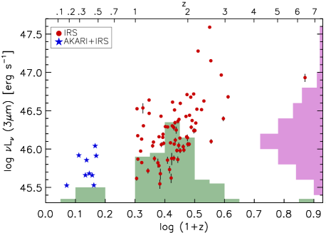
Figure 1: Distribution in the restframe 3 µm luminosity vs redshift plane for the sources in our sample. The solid histograms represent the number counts in same-sized bins of $\log$(1+$z$) and $\log$ $\nu L_{\nu}$(3µm).

3 Stitching

We stitch the different orders in the Spitzer/IRS spectra following the procedure described in Hernán-Caballero et al. (2016). Very briefly, we take the LL2 spectrum as reference and scale the three SL modules to match the SL1 and LL2 spectra in the overlap region. Further adjustments are made to the scaling factors of SL3 and SL2, if needed. Because the IR emission from the galaxy is outshone by the AGN, which is unresolved in Spitzer observations, differences in aperture size between the SL and LL modules are unimportant and the scaling factors applied are usually close to unity. However, inaccurate slit placement for one of the modules may cause a significant loss in flux, which would translate into a large scaling factor. We find no such cases in our sample.

We also stitch together the AKARI and Spitzer spectra for the 9 low redshift quasars. The AKARI spectra were obtained using a squared slit 1’ wide and extracted in a 1’ $\times$ 7.5” aperture, which includes most of the extended emission from the host galaxy (see Kim et al. 2015 for details). However, the 3.3 µm PAH feature is undetected in the 9 sources, indicating that the AGN overwhelms the emission from the host. A gap of $\sim$0.2 µm between the long wavelength end of the AKARI spectrum and the start of the Spitzer spectrum complicates the stitching. We overcome this by fitting with a straight line the 5.15–7 µm range of the Spitzer spectrum and stitching the AKARI spectrum to its extrapolation at 4.9 µm. The mean (median) value of the scaling factors for the AKARI spectra is 0.997 (1.000), which suggests that the contamination from the host galaxy is negligible. The standard deviation is 0.135, fully consistent with uncertainties of $\sim$10% in the absolute flux calibration of both Spitzer and AKARI spectra.

4 Broadband photometry

In addition to the Spitzer and AKARI spectra, we compiled optical and NIR broadband photometry for the sources in the sample.

We retrieved PSF photometry in the $u$, $g$, $r$, $i$, and $z$ bands from the SDSS DR12 SkyServer. We found matches for 71 of our sources using a 6” search radius. For the remaining 14 sources outside of the sky area covered by SDSS we searched for any available optical photometry in NED. We found measurements at least in the $R$ or $V$ bands for all but two sources. We corrected for Galactic extinction following Schlegel et al. (1998). The median extinction corrections for the $u$, $g$, $r$, $i$, and $z$ bands are 0.051, 0.038, 0.027, 0.020, and 0.015 magnitudes, respectively.

We queried the NASA/IPAC Infrared Science Archive (IRSA) for $JHK$ photometry from the Two Micron All Sky Survey (2MASS; Skrutskie et al. 2006) Point Source Catalog (PSC). Using a search radius of 6” we obtained results for 47 sources (all of them within 2” of the Spitzer/IRS position). We took $JHK$ photometry for 15 additional sources within the SDSS area from the SDSS Data Release 7 (DR7) quasar catalogue (Schneider et al. 2010) and the SDSS Data Release 9 (DR9) quasar catalogue (Pâris et al. 2012). These catalogues contain forced aperture photometry on the 2MASS images at the SDSS coordinates, and include all $>$2$\sigma$ detections (compared to $>$5$\sigma$ for the 2MASS PSC). For 14 sources in the Southern hemisphere we retrieved deeper $JHKs$ photometry from the VISTA Hemisphere Survey (VHS; McMahon et al. 2013) Data Release 3. In addition, we obtained $YJHK$ photometry for 24 sources in the areas covered by the UKIRT Infrared Deep Sky Survey (UKIDSS; Lawrence et al. 2007). Since the VHS and UKIDSS data are deeper than 2MASS, we use them in the cases where both are available. There are 9 sources with no NIR photometry from either VHS, UKIDSS or 2MASS. We searched NED for any NIR measurements from pointed observations and found results for three of them (including one K-band upper limit).

In summary, we obtained measurements in five optical bands for $\sim$85% of the sample, and in 3 to 4 NIR bands for $\sim$90% of the sources. This ensures a robust estimate of the luminosity and optical spectral index of the accretion disk component. For the three sources with only one or two data points in the restframe optical range, we obtain a rough estimate of the disk luminosity by fixing the spectral index (see §6.1).

In addition to optical and NIR fluxes, we retrieved from IRSA photometry in the 3.4, 4.6, 12, and 22 µm bands of the Wide-field Infrared Survey Explorer (WISE; Wright et al. 2010). We obtained measurements for all but one sources. While the longer wavelength WISE data points overlap with the IRS spectra, the 3.4 and 4.6 µm bands are useful to constrain the shape of the restframe 1–2.5 µm SED in the 76 IRS-only $z$$>$1 sources. AKARI and WISE calibrations are tied to Spitzer by having absolute calibrators in common (Cutri et al. 2012). However, the WISE 3.4 µm fluxes are known to be systematically lower by 10 per cent compared to AKARI fluxes (Kim et al. 2015), though the reasons are not well understood. SEDs for all the sources in the sample, including the broadband photometry and the (AKARI+)IRS spectra are shown in Figure 2 and Appendix A.

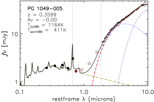
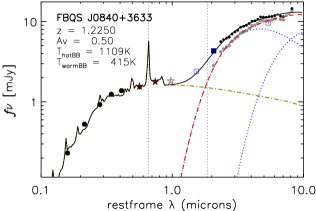
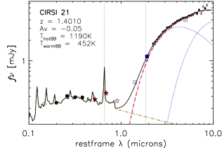
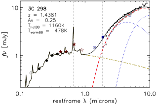
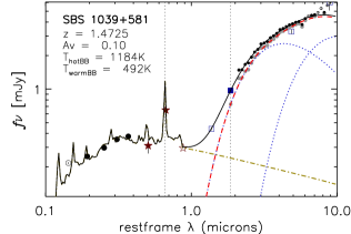
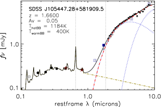
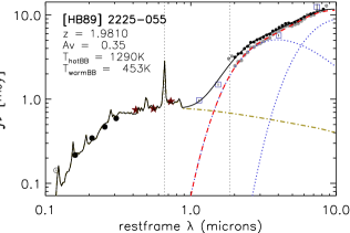
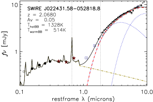
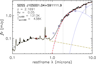
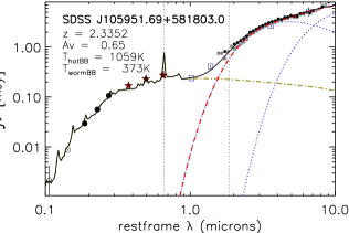
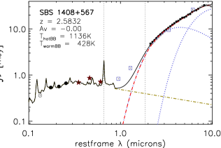
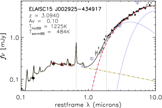
Figure 2: Examples of SEDs and their best fitting disk+dust model for sources in the sample. Circles, stars, and squares represent broadband photometry in the observed-frame optical (from SDSS), NIR (2MASS/UKIDSS/VHS), and MIR (WISE), respectively. Filled symbols indicate bands used to fit the disk component (yellow dot-dashed line). The (AKARI+)IRS spectra resampled at $\lambda$/$\Delta\lambda$ = 20 are shown with small black dots. Grey dots below the (AKARI+)IRS spectra represent the dust spectrum obtained after subtraction of the disk component. The model for the dust spectrum (red dashed line) is the linear combination of two black-bodies at adjustable temperatures (blue dotted lines). The combined disk+dust model is represented by the black solid line. The vertical dotted lines mark the restframe wavelength of the H$\alpha$ and Pa$\alpha$ recombination lines. The entire sample is shown in Appendix A.

5 Optical and NIR spectral indices

We first characterise the optical and NIR segments of the quasar spectra by measuring spectral indices. We define the optical spectral index as:

$$\alpha_{opt}=\frac{\log(f_{0.3}/f_{1})}{\log(1\mu m/0.3\mu m)}$$ (1)

where $f_{0.3}$ and $f_{1}$ are the flux densities at the restframe wavelengths 0.3 and 1 µm. Similarly, we define the NIR spectral index as:

$$\alpha_{NIR}=\frac{\log(f_{1}/f_{3})}{\log(3\mu m/1\mu m)}$$ (2)

with $f_{3}$ being the flux density at restframe 3 µm.

These indices correspond to the exponent $\alpha$ of a power-law of the form: $f_{\nu}$ $\propto$ $\nu^{\alpha}$. Since the observed bands sample different restframe wavelengths depending on the redshift of the source, we use power-law interpolation to obtain $f_{0.3}$ and $f_{1}$ from the broadband photometry. Because the actual SEDs of the quasars are more complex than a simple power-law, we discard interpolations from sparsely sampled SEDs and only consider $f_{0.3}$ and $f_{1}$ measurements in sources with at least one photometric point within the restframe 0.2–0.4 µm and 0.75–1.25 µm ranges, respectively. On the other hand, $f_{3}$ is measured directly on the AKARI or IRS spectrum.

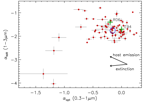
Figure 3: Restframe NIR (1–3 µm) versus optical (0.3–1 µm) spectral indices for the individual sources with valid $f_{0.3}$ and $f_{1}$ measurements. The large open circle marks the median value for the sample, while the large plus signs indicate the values corresponding to the mean quasars SEDs from Richards et al. (2006) and Elvis et al. (1994).

Figure 3 compares $\alpha_{opt}$ and $\alpha_{NIR}$ for the 68 sources with valid measurements. We exclude [HB89] 1700+518, which has an extremely low $\alpha_{opt}$=-3 based on just two photometric measurements in the $V$ and $J$ bands. For the remaining sources, the values of $\alpha_{opt}$ concentrate around the median values $\tilde{\alpha}_{opt}$ = -0.16 and $\tilde{\alpha}_{NIR}$ = -1.76, with standard deviations of 0.25 and 0.36, respectively. This is roughly consistent with the mean SED of 259 SDSS quasars with Spitzer/IRAC detections from Richards et al. (2006) ($\alpha_{opt}$=-0.2, $\alpha_{NIR}$=-1.4) and the radio-quiet AGN template from Elvis et al. (1994) ($\alpha_{opt}$=0.0, $\alpha_{NIR}$=-1.7).

The dispersion in $\alpha_{opt}$ values, $\sigma$($\alpha_{opt}$) = 0.25, is consistent with that found by Richards et al. (2001) in a much larger sample of SDSS quasars. Several factors may contribute to this dispersion: variations in the intrinsic spectral index of the disk emission, extinction by material in the nuclear region, in the host galaxy, or in other galaxies along the line of sight, and contamination by emission from the host galaxy. Studies using samples of less luminous quasars have found significantly higher dispersion (e.g. Hao et al. 2010; Bongiorno et al. 2012), that is interpreted as caused by a combination of extinction and contamination by stellar emission in the host galaxy. However, the latter is unlikely to contribute significantly in our sample: assuming that the host galaxy has a typical stellar mass of 10¹¹ M_⊙ and a Salpeter (1955) Initial Mass Function, its restframe 3 µm luminosity is $\sim$10^43.5 erg s^-1, or 1% of our luminosity threshold. Even at 1 µm, where the fractional contribution from the host should be highest, the contamination from stellar emission would be only $\lesssim$10% of the observed flux for the less luminous quasar of the sample. Furthermore, while extinction increases both $\alpha_{opt}$ and $\alpha_{NIR}$ (the latter by a much smaller amount), stellar emission modifies them by quantities that are comparable in magnitude but opposite in direction (see arrows in Figure 3). As a consequence, an anticorrelation between both indices is observed in samples with significant levels of contamination by stellar emission (Hao et al. 2010; Bongiorno et al. 2012). The lack of correlation in our sample confirms our expectation that there is no significant contamination from the host galaxy at these AGN luminosities. Therefore, the dispersion in $\alpha_{opt}$ in our sample must arise from differences in the intrinsic slope and/or the extinction level affecting the quasar continuum. However, it is difficult to tell them apart, because both of them modify optical spectra in similar ways. Recently, Krawczyk et al. (2015) used a bayesian marginalisation method to break the degeneracy and estimated the intrinsic dispersion in the optical spectral index of SDSS quasars at $\sim$0.2, suggesting that this would be the dominant factor.

Since the impact of extinction is much lower at NIR wavelengths and we rule out a significant contamination by the host galaxy, the dispersion in $\alpha_{NIR}$ must be caused by either differences in the SED of the dust emission or differences in the relative luminosity of the disk and dust components. The former would be caused by variation in the distribution of temperatures of the hot dust grains at small radii, while the later depends mostly on the geometrical covering factor and the viewing angle. To quantify the source-to-source variation in the SED of the dust, we need to remove first the contribution from the disk at NIR wavelengths. This is the subject of the next section.

We define the NIR-to-optical luminosity ratio as $r_{NO}$ = $\nu L_{\nu}$(3µm)/$\nu L_{\nu}$(0.5 µm), which can be considered as a proxy for the dust to disk luminosity ratio, a measure of the ‘apparent’ covering factor of the dust (Mor et al. 2009; Alonso-Herrero et al. 2011; Stalevski et al. 2016). Because $\lambda$ = 0.5 µm and $\lambda$ = 3 µm are both safely distant from the $\sim$1.6 µm peak of the stellar emission, this ratio is insensitive to a small contamination from the host galaxy.

Figure 4 shows a loose but strongly significant ($>$3$\sigma)$ anti-correlation between $\alpha_{opt}$ and $r_{NO}$. There are two factors that likely contribute to redder $\alpha_{opt}$ in sources with higher $r_{NO}$. The first one is increased contribution from the dust to the 1 µm emission due to higher relative luminosity of the dust component (see Figure 5). The second is increased reddening of the disk component due to higher dust column density in the line of sight towards the disk. The latter is supported by a clear correlation between the MIR-to-UV flux ratio and the slope of the UV spectrum (Ma & Wang 2013), and the increase in the average geometrical covering factor along the sequence of Seyfert types 1, 1.8–1.9, and 2 (Mateos et al. 2016).

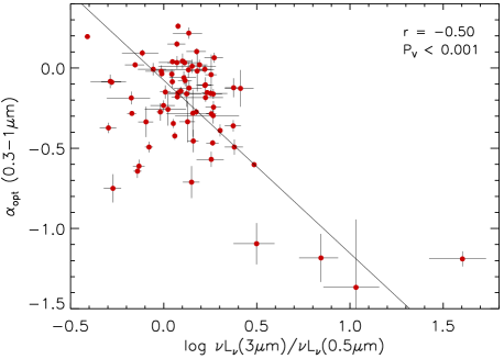
Figure 4: Restframe optical (0.3–1 µm) spectral index versus NIR-to-optical luminosity ratio ($r_{NO}$). The solid line marks the bisector of the X vs Y and Y vs X fits. $r$ and $P_{v}$ represent, respectively, the weighted correlation coefficient and the probability of finding such a high (absolute) value of $r$ if the two variables are uncorrelated.

6 Modelling of the continuum emission

The temperature of silicate and graphite grains, believed to be the main ingredients of dust around AGN, is limited by sublimation to $\lesssim$1500 K. Therefore, the restframe UV and optical emission of the dust is negligible, and nearly all the continuum emission at $\lambda$$<$0.85 µm arises in the accretion disk. The relative contribution of the disk to the total emission is expected to decline quickly at $\lambda$$>$1 µm due to steeply rising emission from the dust. However, emission from the accretion disk could still be significant at 2–3 µm.

The shape of the NIR SED of the disk is uncertain due to the difficulty in disentangling the emission from the dust, but both theoretical considerations (e.g. Hubeny et al. 2001) and polarized light observations (Kishimoto et al. 2008), favour power-law SEDs with $\alpha$$\sim$1/3 at NIR wavelengths. A power-law extension of the rest-frame optical disk emission into the NIR is a common assumption for the primary source that is used as input for radiative transfer codes that model the torus emission (e.g. Granato & Danese 1994; Nenkova et al. 2002; Fritz et al. 2006; Stalevski et al. 2012), but it is not universal. In particular, some torus models assume a steep fall of the disk spectrum longwards of 1 µm (e.g. Hönig et al. 2006; Nenkova et al. 2008; Siebenmorgen et al. 2015) which makes its NIR emission negligible compared to that of the torus even for face-on views. Since the NIR range contributes a small fraction of the bolometric emission from the primary source, its impact on the spectrum of the dust-reprocessed radiation must be small. However, the NIR SED of the total AGN emission (disk+dust) depends substantially on the spectral shape assumed for the NIR spectrum of the disk (Feltre et al. 2012). In particular, modelling with steeply falling disk emission at $\lambda$$>$1 µm could contribute to the NIR excess observed in type 1 AGN relative to the best-fitting disk+torus model (e.g. Mor et al. 2009; Alonso-Herrero et al. 2011). In a sample of 26 Palomar-Green quasars, Mor et al. (2009) found that their Spitzer/IRS spectra cannot be reproduced with a combination of the clumpy torus models from Nenkova et al. (2008) and emission from the narrow line region, and a third component of very hot dust ($T$$\sim$1400 K) is required. In the analysis of the Spitzer/IRS spectra of 25 $z$$\sim$2 quasars, Deo et al. (2011) concluded that the additional hot dust component is required for fitting simultaneously the NIR SED and the $\sim$10 µm silicate feature with clumpy torus models. However, Mateos et al. (2015) were able to fit the nuclear SEDs of X-ray selected quasars using a non-truncated disk and the torus models from Nenkova et al. (2008), with no NIR excesses.

6.1 Emission from the accretion disk

Previous studies modelled the optical emission of the disk with a single power-law with the form $f_{\nu}\propto\nu^{\alpha}$ of adjustable (e.g.: Kim et al. 2015) or fixed (e.g.: Mateos et al. 2015) spectral index $\alpha$. While this usually provides acceptable fits in the restframe optical range (0.3–0.85 µm), its extrapolation into the restframe UV cannot reproduce the usually much redder observed SED (this change in slope originates the so-called big blue bump at $\sim$0.3 µm), and a double power-law is often preferred. Another difficulty in the case of broadband photometry is introduced by the contamination from strong emission lines like H_α. Since the number of photometric data points at restframe UV to optical wavelengths in our sources is between 2 and 7, a model with two power-laws plus emission lines would have too many free parameters. Accordingly, we choose to use instead a single empirical quasar template. To reproduce the variety of optical spectral indices in our sample, we allow for varying amount of extinction to affect the template. Therefore our model has only two free parameters: the normalisation of the template and $A_{V}$.

We use the extinction law of the Small Magellanic Cloud Bar (Gordon et al. 2003), which is often preferred for quasars because it lacks the 2175Å absorption feature. We choose the composite quasar spectrum from Shen (2016) as our universal UV+optical quasar template. Unlike previous quasar composites (e.g. Vanden Berk et al. 2001), the Shen composite is derived from observed-frame NIR spectroscopy of luminous ($L_{\rm{bol}}$ = 10^46.2-48.2 erg s^-1) high redshift (1.5$<z<$3.5) quasars. This composite is significantly bluer in the optical range compared to that from Vanden Berk. Its slope at $\lambda$$>$0.3 µm is close to $\alpha$=1/3, and therefore its extension into the NIR with the same slope is consistent with theoretical expectations. Redwards of the H_α line the composite spectrum is somewhat redder than $\alpha$=1/3. Because this could indicate some residual contamination from the host or the onset of the dust emission, we extrapolate the template into the NIR range by scaling an $\alpha$=1/3 power-law to fit the 0.3–0.6 µm range.

We obtain reddened versions of the quasar template by applying different levels of extinction, from A_V = -0.4 to A_V = 1.0 in steps of 0.05. Negative values of A_V are needed to obtain good fits for some of the quasars with bluer continua, since the template is the average of many quasar spectra affected by different levels of extinction. In this respect, the A_V values should be considered as relative to that of the average template.

We find the best fitting template for the disk of each quasar by least-squares fitting the photometric points corresponding to bands with effective wavelengths between 0.15 and 0.85 µm in the restframe. This means that we use up to 7 bands from SDSS and 2MASS/UKIDSS/VHS to fit a model that effectively has only two free parameters (A_V and the normalisation constant for the template). For the three sources with only one or two data points in the fitting range we force A_V=0. We also force A_V=0 for five additional sources with three or four data points but all of them at $\lambda_{rest}<$4000Å. The values of the ‘relative’ extinction obtained (considering only the 77 sources with free A_V) range from A_V = -0.1 to 0.9 mag (median value: 0.05), but 90% of them are within the [-0.1,0.4] interval. Given the simplicity of the model, the quality of the fits is remarkable (see Figure 2), with residuals apparently dominated by the varying strengths of the broad emission lines.

The extension into the restframe NIR of the disk model allows to estimate the contribution from the accretion disk to the observed restframe NIR emission, $r_{disk}(\lambda)$ = $f_{\nu,disk}(\lambda)$/$f_{\nu,total}(\lambda)$. Values vary widely from source to source due to differences in the relative luminosity of the disk and dust components, but they show a consistent and rapid decline in the relative contribution of the disk to the total emission with increasing wavelength (Figure 5). The median values of $r_{disk}(\lambda)$ at the restframe wavelengths 1, 2, and 3 µm are 63%, 17%, and 8%, respectively.

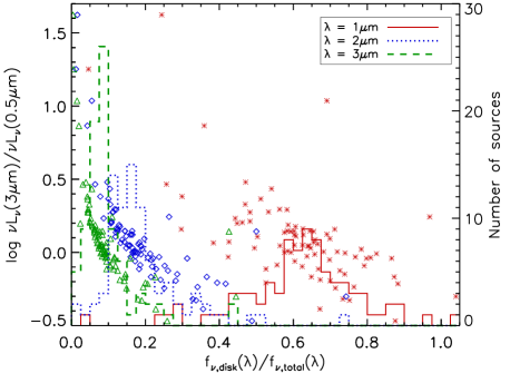
Figure 5: Relation between the NIR-to-optical luminosity ratio, $r_{NO}$ = $\nu L_{\nu}$(3µm)/$\nu L_{\nu}$(0.5µm), and the estimated contribution from the disk to the total emission, $r_{disk}(\lambda)$, at restframe 1µm (red stars), 2 µm (blue diamonds), and 3µm (green triangles). The histograms show the distributions of $r_{disk}(\lambda)$ for each of the three restframe NIR wavelengths.

6.2 Emission from the dust

Assuming that the NIR and MIR emission from the host galaxy is negligible, all the flux remaining after subtraction of the disk component corresponds to reprocessed radiation from dust heated by the AGN. This dust may be located in a toroidal structure that surrounds the central engine (the so-called dusty torus) or in the narrow-line region, or both. Since our aim is not to test physical models of the AGN dust emission, but to characterise the observed NIR spectrum in a geometry-agnostic way, we resort to fitting a simple analytical function defined as the sum of two blackbody profiles:

$$f_{\nu}(\lambda)=aB_{\nu}(\lambda,T_{hot})+bB_{\nu}(\lambda,T_{warm})$$ (3)

where the temperatures $T_{hot}$ and $T_{warm}$ are free to vary within the intervals 850–2000 K and 150–900 K, respectively, and the normalisation factors $a$ and $b$ must be non-negative.

In the fit, we use photometric and spectroscopic data points within the 1.7–8.4 µm range in the restframe. This is to avoid complications due to possible residual contamination from the host galaxy or the disk and the onset of the 10 µm silicate feature at shorter and longer wavelengths, respectively. We also remove from the fit data points in the 6.10–6.45 µm and 7.3–8.1 µm intervals to prevent any contamination from the PAH features. Prior to the fit, we remove the disk component derived in the previous section and resample the (AKARI+)IRS spectrum with a uniform resolution $R$ = $\lambda$ /$\Delta\lambda$ = 20 (a factor 2–4 lower than the original data) in order to improve the signal to noise ratio (SNR).

The best fitting values of the four free parameters ($a$, $b$, $T_{hot}$, $T_{warm}$) are calculated using the IDL routine MPFIT (Markwardt 2009). We repeat the fit 100 times for each source with different initial values for $T_{hot}$ and $T_{warm}$ to ensure that the fit converges to a global minimum. We obtain remarkably good fits for all sources, with reduced $\chi^{2}$ values around unity.

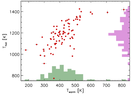
Figure 6: Relation between the temperatures for the hot and warm dust components in individual sources. Error bars indicate the nominal 1-$\sigma$ uncertainties derived by MPFIT. The solid histograms represent the distribution of $T_{hot}$ and $T_{warm}$ in the sample.

Figure 6 shows the temperatures of the hot and warm dust components of the best fitting model for each individual source. Values of $T_{hot}$ range between 900 and 1425 K (mean: 1188 K, median: 1190 K). The only outlier is SDSS J100552.63+493447.9 at $T_{hot}$ = 773 K, which has extremely red optical and NIR spectra. The distribution for $T_{warm}$ ranges from 180 to 815 K (mean: 424 K, median: 415 K), but only 5 sources are outside the 250–550 range.

The ratio between the bolometric luminosity of the hot and warm components ($r_{HW}$) ranges from 0.3 to 4.4 (mean: 1.66, median: 1.54). There is a correlation between the temperatures of the hot and warm dust components, which is probably a consequence of modelling a continuous distribution of temperatures with only two discrete values. However, neither $T_{hot}$ or $T_{warm}$ correlate with $r_{HW}$, $\alpha_{NIR}$, $r_{NO}$ or $A_{V}$.

The best fitting two-blackbody model for the disk-subtracted continuum and the combined disk+dust models are shown in Figure 2. The disk+dust model reproduces correctly the optical SED and the IR spectrum within the restframe 1.7–8.4 µm interval used to adjust the parameters of the blackbody components. However, the measurements within the $\sim$0.9–1.7 µm range (which were excluded from both the disk and dust modelling) are systematically underestimated by the disk+dust model.

To understand why the broadband restframe NIR photometry departs from our otherwise succesful model, we compute the relative excess at 1.2 µm as: $e_{NIR}$ = ($f_{obs}$ - $f_{model}$)/$f_{model}$, where $f_{obs}$ is the flux density at restframe 1.2 µm interpolated in the observed SED and $f_{model}$ is the prediction from the best-fitting disk+dust model. Because the wavelength coverage in the restframe 1.0–1.5 µm range is sparse in many sources, we avoid biasing our analysis by considering only sources with at least one photometric point in the 1.1–1.3 µm interval or, alternatively, one in each of the intervals 1.0–1.2 and 1.2–1.4 µm. There are 46 such sources in the sample. Their relative excesses range between 3% and 198% (median: 36%).

We consider three possible scenarios for the origin of this excess: i) contamination by stellar emission in the host galaxy, ii) underestimation of the NIR emission of the accretion disk, iii) underestimation of the NIR emission of the dust. To identify the more likely one, we look for correlations with the 3 µm luminosity and the NIR-to-optical luminosity ratio (Figure 7). If the host galaxy were responsible for the excess we should find an anti-correlation between $e_{NIR}$ and $\nu L_{\nu}$(3µm), but we find none. The correlation between $e_{NIR}$ and $r_{NO}$ should be negative (anti-correlation) if the excess originated in the disk, and positive if it belonged to the dust. We find a clear positive correlation (Figure 7, center panel), and therefore scenario iii) is preferred.

Since the emission at $\lambda$$>$1.7 µm is well reproduced by the model, the excess at shorter wavelengths must originate in very hot dust at or near the sublimation temperature. The fitting procedure is largely blind to such dust because data points at longer wavelengths dominate the fit. This arguably favours lower values for $T_{hot}$ than would be obtained using the full NIR SED. Such interpretation is backed by the loose but strongly significant anti-correlation between $e_{NIR}$ and $T_{hot}$ (Figure 7, right panel), which shows that strong NIR excesses are more likely in sources with colder $T_{hot}$ values.

To check whether a two blackbody model can also reproduce the $\lambda$$<$1.7 µm spectrum of the dust, we repeat the fits including also data points in the restframe 1.2–1.7 µm range. We find that the resulting higher $T_{hot}$ values decrease the 1.2 µm excess by $\sim$50% on average, but only at the expense of significantly worse fits at longer wavelengths. In some cases $T_{hot}$ gets extreme high values up to 1750 K. This, together with the large dispersion of the excesses for any given value of $T_{hot}$ shown in Figure 7 suggest that a single temperature hot blackbody component cannot reproduce accurately the entire NIR spectrum of the dust.

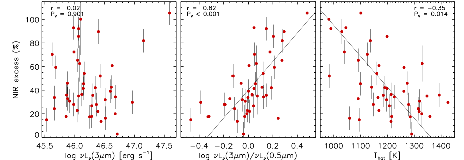
Figure 7: Correlations (or lack thereof) of the relative excess at 1.2 µm after subtraction of the best-fitting disk+dust model with the restframe 3 µm monochromatic luminosity (left), the NIR-to-optical luminosity ratio (centre), and the temperature of the hot blackbody component (right). The error-weighted Pearson correlation coefficient and p-value (probability of obtaining a value of $r$ greater than observed if the null hypothesis -no correlation- is true) are given in the top left corner of each panel. The plots exclude the outlier [HB89] 1700+518.

We note that while the optical, NIR, and MIR data were obtained at different epochs, sometimes several years apart, our results are probably not affected by variability in the quasar emission. It is well established that the amplitude of the optical variability is strongly anti-correlated to the quasar luminosity (e.g.: Hook et al. 1994; Meusinger & Weiss 2013; Kozłowski 2016) and for the luminosity of our sample the amplitude is expected to be only $\sim$0.1 mag on timescales of years, comparable to the photometric uncertainty of our data. In addition, the component sampled by the MIR data (black body) is energetically decoupled from the disk component in our fitting method (i.e. there is no energy balance, since this is not a physical model). We have evaluated the impact of optical variability in the reddening determination by increasing/decreasing the SDSS fluxes by 10% and repeating the fits with the disk model. All the sources obtain their new best fit with the same A_V as before or $\pm$0.05 magnitudes, indicating that the change in A_V is smaller than our discretization step.

7 Composite spectra

Further insight into the origin of variation in the NIR spectrum of quasars can be gained from the comparison of the composite spectra of adequately selected subsamples. As composite spectra are model independent, this is a complementary approach to the model-fitting in the previous section.

We obtain the composite (AKARI+)IRS spectrum of the whole sample with the following procedure:

First, the spectra are shifted to the rest-frame and resampled to a common grid of wavelengths. Each point in the resampled grid represents an equal-sized interval in log($\lambda$). We normalise the spectra at a given restframe wavelength. For every wavelength in the grid, we obtain the flux of the composite spectrum as the weighted average of the fluxes of the individual sources, excluding the sources with no data at that wavelength. The shape of this preliminary composite spectrum depends on the normalisation wavelength, since a normalisation at short wavelengths increases the relative contribution of the redder spectra at long wavelengths, and therefore overestimates the slope of the continuum. Conversely, normalisation at long wavelengths favours the bluer ones and leads to underestimation of the continuum slope. To compensate for this, we use the composite spectrum as a template to re-normalise the individual spectra by fitting with a least squares procedure the entire spectral range covered by each of them. We combine the re-normalised spectra using the same weighted average procedure to obtain a new composite spectrum, and iterate. We find that changes in the composite spectrum are negligible after the second or third iterations, and the wavelength chosen for the initial normalisation has a negligible impact on the final result (see Figure 8).

The uncertainties in the composite spectrum are computed with a bootstrap resampling: we obtain composite spectra for 100 random samples extracted with replacement from the whole sample, each containing 85 sources. Then the 1-$\sigma$ confidence interval for the composite spectrum at each wavelength is given by the 16^th and 84^th percentiles of the distribution for the 100 bootstrap iterations.

The composite spectrum shows that the 3–7 µm SED is well reproduced by a power-law with $\alpha$ = -1. This is in agreement with previous estimates of the MIR spectral index of high redshift quasars (e.g. Lutz et al. 2008; Hernán-Caballero et al. 2009) as well as low redshift ones (e.g. Netzer et al. 2007). However, at shorter wavelengths the continuum slope is increasingly steep and interrupted only by a prominent Paschen $\alpha$ line. Other hydrogen recombination lines as well as PAH features can also be identified in the spectrum (see §8 for a discussion).

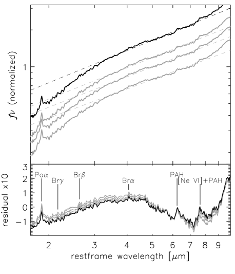
Figure 8: Top panel: final composite spectra after several iterations of the normalisation procedure for initial normalisation at 3 µm (black solid line), or 4, 5, and 7 µm (grey solid lines). The dashed lines represent the best-fitting power-law for each composite in the the 3–7 µm spectral range. Bottom: residuals obtained by subtracting from the composite spectra a power-law with $\alpha$ = -1. Labels mark some significant spectral features.

7.1 Dependence with AGN luminosity

We obtain composite spectra for the subsamples with lower ($\nu L_{\nu}$(3µm) $=$ 10^45.5-46.15 erg s^-1) and higher ($\nu L_{\nu}$(3µm) $>$ 10^46.15 erg s^-1) NIR luminosity, that contain the same number of sources. If the (AKARI+)IRS spectra were contaminated by stellar emission in the host galaxies of the quasars, the impact should be higher in the lower luminosity composite, that would appear bluer at short wavelengths compared to the higher luminosity one. However, we find no significant differences between the two composites (Figure 9). The lack of divergence at short wavelengths reinforces our previous claim that the stellar emission is negligible for the sources in the sample.

At longer wavelengths we find that the divergence is marginally significant around the $\sim$7.7 µm PAH complex. The residual suggests a weaker contribution from star formation to the spectra of more luminous quasars, in agreement with previous results (e.g. Haas et al. 2003; Maiolino et al. 2007; Hernán-Caballero et al. 2009; Barger et al. 2015). If this small divergence is attributed to star formation in the host galaxy, then the entire 2–10 µm spectrum of the quasar itself is independent on the NIR luminosity, at least within the luminosity range of our sample. This is contrary to previous results based on broadband photometry that suggested a luminosity dependence in the NIR-to-MIR quasar SED, and in particular a more prominent 4 µm bump and bluer MIR continuum for the more luminous quasars (Richards et al. 2006; Gallagher et al. 2007).

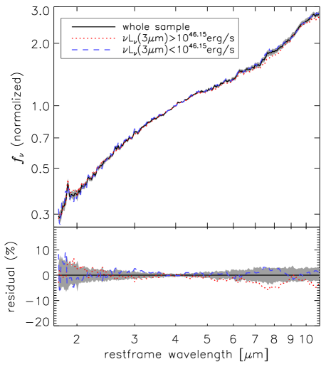
Figure 9: Comparison between the composite spectra for the low and high luminosity subsamples. The shaded area represents the 1-$\sigma$ uncertainty for the composite template of the whole sample. The bottom panel shows the residuals of subtracting the whole sample composite from the high and low luminosity composites, normalised by the flux of the whole sample composite.

7.2 Dependence with the NIR-to-optical luminosity ratio

The uncertain contribution from the accretion disk to the NIR and MIR emission should manifest itself as differences in the composite spectrum between the high $r_{NO}$ and low $r_{NO}$ subsamples, because the contribution from the disk should be higher in the latter. We split the sample into two same-sized subsamples with $r_{NO}$$<$1.3 and $r_{NO}$$>$1.3. We compare their composites in Figure 10. The $r_{NO}$$>$1.3 composite is significantly redder at short wavelengths, consistent with a smaller contribution from the accretion disk to the NIR emission. We also note the lack of a clear Pa$\alpha$ emission line in this composite, which is also expected for a high dust-to-disk luminosity ratio if the luminosity of the hydrogen recombination lines correlates with that of the disk continuum (see §8). If the relative luminosities of the accretion disk and dust were the only factor affecting $r_{NO}$, the two composites should converge to the same spectrum at MIR wavelengths, where the disk contribution is expected to be negligible. However, we find highly significant divergence also at $>$5 µm. The high $r_{NO}$ composite is flatter (more power-law like) and redder than the low $r_{NO}$ one, which presents a blue 5–8 µm continuum and a stronger silicate emission feature. This suggests that the spectrum of the dust component is slightly different in high $r_{NO}$ and low $r_{NO}$ quasars, with a bluer continuum and a more pronounced 4 µm bump in the latter. This is in good qualitative agreement with the results by Mateos et al. (2016) in a large X-ray selected AGN sample, who found redder MIR SEDs for the tori in type 1 AGN with higher geometrical covering factors.

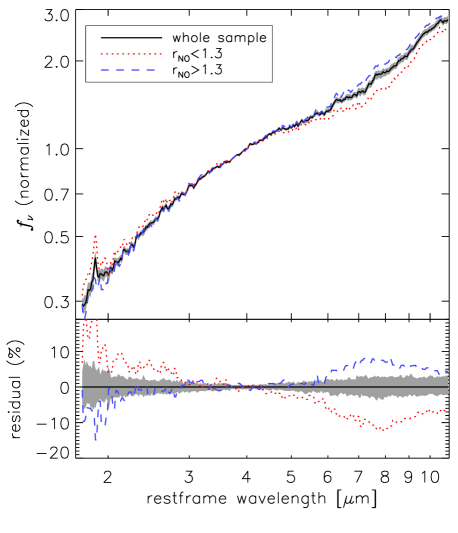
Figure 10: Comparison between the composite spectra for the subsamples with high and low values of the restframe 3 µm to 0.5 µm luminosity ratio, $r_{NO}$. Symbols as in Figure 9.

7.3 Dependence with the optical spectral index

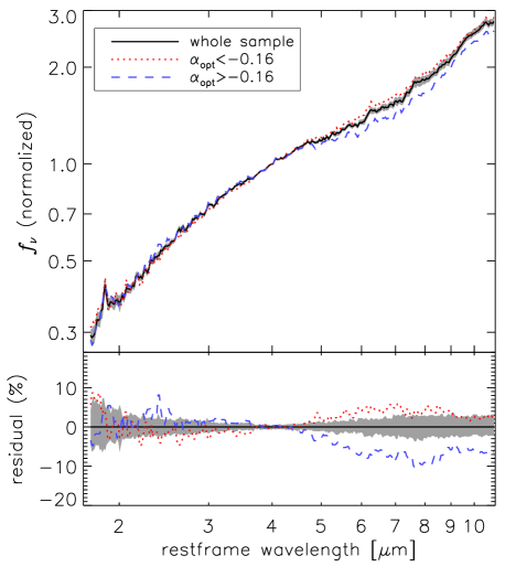
Figure 11: Comparison between the composite spectra for the subsamples with high and low values of the optical spectral index, $\alpha_{opt}$. Symbols as in Figure 9.

Finally, we checked for a dependence of the composite spectrum with $\alpha_{opt}$, that relates on both the intrinsic slope and the extinction affecting the disk component. The composite spectra for $\alpha_{opt}>$-0.16 and $\alpha_{opt}<$-0.16 (Figure 11) are not significantly different at NIR wavelengths. However, there is a clear divergence at $\lambda>$4 µm, with the composite for the blue optical AGN having a more pronounced 4 µm bump and a bluer MIR spectrum. The shape of the residuals resemble that of the high and low $r_{NO}$ composites (except for the collapse in the divergence at $\lambda$$\lesssim$2.5 µm), but the departure from the full sample composite is less pronounced. This suggests that the variation with $\alpha_{opt}$ is mostly an indirect consequence of the variation with $r_{NO}$ enabled by the (weak) correlation between $r_{NO}$ and $\alpha_{opt}$.

7.4 Comparison with other IR composites

We now compare our IR quasar composite spectrum with other composites from the literature with spectral coverage in the $\sim$2–4 µm range (Figure 12).

The composite from Glikman et al. (2006) shows a prominent Paschen $\alpha$ line that is comparable in strength to that in our template, but the continuum longwards of the line is flat (in $\nu f_{\nu}$) while our template shows a prominent 3µm bump. The discrepancy is most likely due to the fact that the $\lambda$$>$2 µm part of their composite is obtained from the noisy L-band spectra of a few sources (between 4 and 15 depending on wavelength). On the other hand, at $\lambda$$\lesssim$2µm the Glikman composite is in good agreement with our composite broadband SED (see §9).

The composite from Hill et al. (2014) was obtained from the Spitzer/IRS spectra of 61 SDSS quasars with 5.6 µm luminosities between 10^44.8 and 10^46.1 erg s^-1. We have normalised their composite to match ours at 5.6 µm, where their coverage is highest. The two spectra have similar shapes in the 4–11 µm range. The main difference is the larger EW of the 6.2 µm and 7.7 µm PAH features in their composite, probably caused by a lower by $\sim$0.5 dex median luminosity compared to our sample ($\sim$10^45.5 erg s^-1 vs 10^46.15 erg s^-1). Their $\lambda$$<$4 µm spectrum shows a substantially more pronounced bump compared to ours. The differences may be due to the low number of objects contributing to this part of their composite. That might also be the cause of the spikes at $\sim$2.5 and $\sim$3.1 µm, which do not match any known emission feature.

The composite AKARI spectrum of 48 PG QSOs from Kim et al. (2015) shows a better match to the 2–4 µm range of our composite, with departures only at the extremes of the range. Our IR composite is therefore consistent with the others in the ranges where they are the more robust. This highlights the homogeneity of optically selected quasar samples and suggests that previous discrepancies in the average quasar spectrum were mostly due to observational limitations.

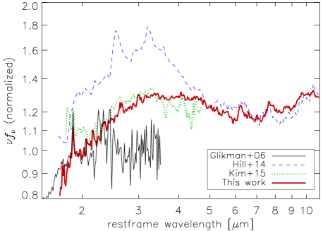
Figure 12: Comparison of composite infrared spectra of quasars. The thin black line is the composite NIR spectrum of 27 low redshift ($z$$<$0.42) bright (K_s$<$14.5) SDSS quasars from Glikman et al. (2006). The blue dashed line is the composite Spitzer/IRS spectrum of luminous ($\log$(L_5.6μm/erg s^-1) = 44.8–46.1) SDSS quasars from Hill et al. (2014). The green dotted line is the composite AKARI spectrum of 48 PG QSOs from Kim et al. (2015). The thick red line is our own composite quasar spectrum.

8 Emission lines

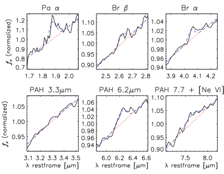
Figure 13: Emission lines and PAH features observed in the composite quasar spectrum for the full sample. The continuum (dotted line) and feature (dashed line) are modelled with a straight line and a Gaussian profile, respectively.

At the spectral resolution of the Spitzer/IRS low resolution modules (R$\sim$60–120) and AKARI (R$\sim$60) the emission lines of quasars are usually washed out by the strong continuum emission in individual spectra. Even the broader PAH features are undetected in most quasars because they contribute a tiny fraction of the flux density per resolution element, and therefore get masked by photometric noise. However, by averaging many spectra, we obtain a very high SNR in the composite, which allows to detect several emission lines and PAH bands.

We measure the strength of the emission lines and PAH features in the composite spectrum by fitting simultaneously a Gaussian profile and a linear local continuum. We set free the height and width of the Gaussian but fix the central wavelength at the theoretical value. The width of the fitting interval (between 0.4 and 1.2 µm) is enough for a good determination of the continuum and not as large as to make curvature effects important. Figure 13 shows the best fits for the hydrogen recombination lines Paschen $\alpha$, Bracket $\alpha$, and Bracket $\beta$, as well as the PAH features at 3.3, 6.2 and 7.7 µm.

We estimate uncertainties for the line strengths using the distribution of the measured values in 100 random composite spectra obtained through bootstrap resampling of the full sample. The median values and 1-$\sigma$ confidence intervals (percentiles 16^th and 84^th) for the equivalent width and the FWHM are given in Table 2. All the features except the 3.3 µm PAH are detected at the $>$3$\sigma$ level. The strongest detections correspond to the 7.7 µm PAH complex ($\sim$4.7$\sigma$) that includes the [Ne vi] 7.642 µm line, and Paschen $\alpha$, that is detected at the $\sim$4.5$\sigma$ level in spite of having only 25 sources (5 at $z$$<$1 and 20 at $z$$>$1) with enough spectral coverage to observe it.

The three hydrogen lines have comparable values for the FWHM ($\sim$0.065-0.075 µm). They correspond to velocity dispersions between 10000 km/s for Paschen $\alpha$ and 5000 km/s for Bracket $\alpha$. These values are not corrected for the instrumental broadening, which in the case of IRS spectra is $\sim$4000 km/s for Paschen $\alpha$ and $\sim$2000 km/s for Bracket $\alpha$. Also, the uncertainty in the wavelength calibration and the redshifts of the individual sources contributing to the composites may produce some additional broadening. Therefore we consider these values to be fairly consistent with expectations for the composite spectra of luminous QSOs.

Since the EW is insensitive to the normalisation, the EW of features in the composite spectrum represent the average EW in the individual spectra. We obtain an EW of 124$\pm$30 Å and 17$\pm$4 Å for the Paschen $\alpha$ and Bracket $\alpha$ lines, respectively. The Paschen $\alpha$ EW is consistent with a mean value of 104$\pm$43 Å found by Landt et al. (2008) for a sample of 23 well known type 1 AGN at $z$$<$0.4 with NIR spectra from the NASA Infrared Telescope Facility. It is also in good agreement with the EW = 120 Å found by Soifer et al. (2004) for the Paschen $\alpha$ line in the Spitzer/IRS spectrum of the strongly lensed $z$=3.92 quasar APM 08279+5255, that was not included in our sample. In contrast, Glikman et al. (2006) give a Paschen $\alpha$ EW of just 12.7 Å for the composite spectrum of 27 bright ($K_{s}$$<$14.5) SDSS quasars at $z$$<$0.42. However, we have re-measured the EW of several lines on their composite spectrum and found that the values listed in their Table 6 are systematically underestimated by a factor 3-4. Our estimate of the Paschen $\alpha$ EW on their template is 55 Å. This is still a factor $\sim$2 lower than the value found in our composite, which is striking. Significant contamination from the stellar emission of the host galaxy is ruled out by Glikman et al. (2006), who estimate a contribution from the host galaxy of just $\sim$6% at 1 µm. Higher average extinction in the BLR for the Glikman et al. (2006) sample is also unlikely because their quasars were selected to be blue and with little to no extinction, and the amount of extinction required to halve the Paschen $\alpha$ flux would cause a factor $\sim$40 decrease in H$\alpha$. We can also rule out a reduction in the Paschen $\alpha$ EW due to stronger dust emission relative to the disk in their sample, since the NIR-to-optical ratio (as measured by $r_{NO}$) is in fact slightly higher in our sample. Therefore, the difference in EW suggests that the Paschen $\alpha$ line in our sample is a factor $\sim$2 more luminous relative to both the disk and the dust continuum emissions.

The composite broadband SED (connected dots in Figure 14) also shows tentative evidence for strong Paschen $\beta$ 1.282 µm and/or Paschen $\gamma$ 1.094 µm in the form of a small peak at $\sim$1.2 µm (see §9). Futher observations in the restframe NIR with the NIRSpec and MIRI instruments onboard JWST will be essential to confirm and understand these results.

9 Quasar template

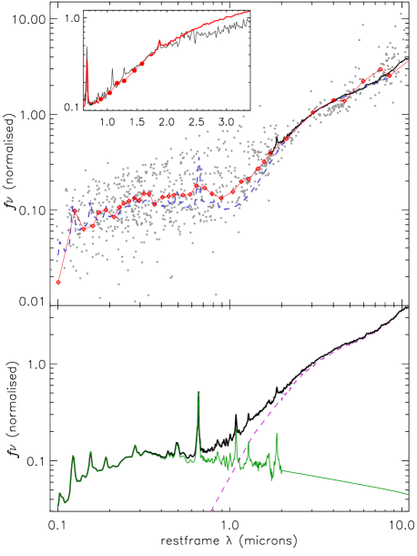
Figure 14: Generation of a quasar template from our sample. Top panel: the (AKARI+)IRS composite spectrum (solid black line) is extended to shorter wavelengths using the 0.85–1.7 µm range of the broadband SED composite (red connected dots), and the $<$0.85 µm range of the model composite (blue dashed line). The small grey dots represent the broadband photometry of individual sources normalised at restframe 3 µm. Inset plot: comparison of our template (red thick line and connected dots) with the quasar composite from Glikman et al. (2006) (black thin line). Bottom panel: The thick black line is the final quasar template after replacing the 0.85–1.7µm range from our broadband SED with the Glikman composite. We also obtain templates for the dust emission (pink dashed line) and the disk emission (including emission lines; green thin line). See text for details.

In this section we present a new template for the 0.1–11µm spectrum of quasars based on our sample. Since the composite (AKARI+)IRS spectrum constructed in §7 is defined only at $\lambda$$>$1.7 µm, we also build composites from the broadband SEDs and the best-fitting disk+dust models of the individual sources. The broadband SED composite is obtained by normalising the individual SEDs at restframe 3.0 µm and obtaining median fluxes in bins containing 20 data points each. The model composite is the median of the individual best-fitting models, after normalisation at 3.0 µm.

The top panel in Figure 14 shows the three composites. There is a good correspondence between the (AKARI+)IRS (black solid line) and the broadband (connected dots) composites, in spite of the poor sampling of the broadband SED at $\lambda$$>$2 µm. The broadband SED also reproduces accurately the composite model in the optical and UV ranges (which is ultimately derived from the empirical quasar template from Shen (2016), as described in §6.1), in spite of the large dispersion among individual sources that is a consequence of their varying NIR-to-optical luminosity ratios. The main discrepancy is at $\sim$1.2 µm, where the model underpredicts the flux in the broadband SED (see §6.2 for a discussion).

We generate a quasar template by stitching together the $\lambda$=1.7–11 µm composite (AKARI+)IRS spectrum, the 0.85–1.7 µm interval of the composite broadband SED, and the 0.10–0.85 µm section of the composite model. We compare the 0.6–3.4µm range of this template with the composite spectrum from Glikman et al. (2006) in the inset in Figure 14. While the Glikman composite diverges from ours at $\lambda$$>$2 µm, probably because it relies on noisy L-band spectra of a few sources (see §7.4), the two templates are in good agreement for $\lambda$$\lesssim$2µm in spite of the poor sampling of our broadband SED. This confirms the robustness of our broadband NIR data and suggests that both samples have equally low contamination by the host galaxy emission. We capitalise on this good agreement by replacing the 0.85–1.7µm section of our template with the Glikman composite, which includes several interesting emission lines in this range. Therefore our final 0.1–11µm template is derived entirely from spectroscopic observations.

We also obtain separate templates for the dust and the disk (plus emission lines) as follows: We subtract from the full template the composite model spectrum of the disk component in the individual sources. This provides a first approximation to the spectrum of the dust, which is however contaminated by the NIR emission lines since they were not included in our power-law extrapolation of the Shen template. We remove the emission lines from this preliminary dust template by fitting a broken power-law in the $\lambda$$<$2µm range, excluding the intervals affected by the main emission lines: He ii 1.083 µm + Pa$\gamma$ 1.094 µm, Pa$\beta$ 1.282 µm, and Pa$\alpha$ 1.876 µm. The best fit is obtained for a spectral index $\alpha$ = -2.3 between 1.35 and 2.0 µm and a steeper $\alpha$=-3.2 for $\lambda$$<$1.35µm. Finally we subtract this line-free dust template from the full template to obtain a template for the disk emission that now includes the NIR emission lines. The final disk, dust, and full (disk+dust) templates are shown in the bottom panel of Figure 14 and in Table 3.

10 Summary and conclusions

We present the analysis of a sample of 85 luminous ($\log$($\nu L_{\nu}$(3µm)/erg s^-1) = 45.5–47.5) quasars with available restframe NIR and MIR spectroscopy from AKARI and Spitzer/IRS. We complement the spectroscopic data with broadband photometry from SDSS, 2MASS, UKIDSS, and WISE.

The optical and NIR spectral indices of individual sources concentrate at $\alpha_{opt}$=-0.2 and $\alpha_{NIR}$=-1.75, consistent with the quasar templates from Elvis et al. (1994) and Richards et al. (2006). The small dispersion and lack of correlation between the two indices indicate little to no contamination from the stellar population in the host galaxy. We find the restframe UV and optical broadband SEDs of individual sources to be well reproduced by a single quasar template affected by varying levels of extinction. The analytical extrapolation of this template into the NIR as a power-law with $\alpha$=1/3, together with a simple model for the dust emission consisting on the superposition of two blackbodies, provides good fits for the restframe 1.7–8.4 µm spectrum in all sources, with temperatures for the hot blackbody component ranging between 950 and 1450 K. However, the extrapolation at shorter wavelengths of the best fitting model systematically underpredicts the observed flux near the 1 µm minimum of the quasar SED. We find a correlation between the relative strength of this NIR excess and the NIR to optical luminosity ratio ($r_{NO}$), which indicates that the excess is not related to the disk or host galaxy emissions but originates in dust near the sublimation radius. We combine the (AKARI+)IRS spectra of the individual sources to obtain composite spectra with very high SNR. The signal is high enough to detect several NIR hydrogen recombination lines and PAH features, in spite of their extremely low EW. Contrary to previous results, we find no luminosity dependence in the NIR and MIR shape of the quasar spectrum within the range of our sample. We find a small but highly significant dependence with $r_{NO}$, which suggests that quasars with higher apparent covering factors have a redder NIR-to-MIR SED and a less prominent silicate emission feature. We generate a new spectroscopic quasar template from our sample that covers the restframe range 0.1–11 µm. We also produce templates for the disk and dust components. Comparison of our template with other spectroscopic quasar composites shows that previous composites are less reliable in the 2–4 µm range, probably due to the low number of sources with sufficient spectral coverage and/or noisy data in this range. Our template is the first one that provides a detailed and consistent view of the IR emission on either sides of the 4 µm bump.

Appendix A SEDs and model fits for individual sources

Table 1: Sources included in the quasar sample.

AOR ID	Source name	RA(J2000.0)	Dec(J2000.0)	$z$	$\nu L_{\nu}$(3µm)		opt. phot.	NIR phot.	spec. class	spec. ref.
4734464_0	PG 1116+215	169.78622	21.32168	0.1765	3.35$\pm$	0.026	SDSS	2MASS	QSO	SDSS DR12
4675840_0	[HB89] 1700+518	255.35359	51.82235	0.2920	8.29$\pm$	0.032	NED	2MASS	BAL QSO	Schmidt & Hines (1999)
14192640_0	PG 1049-005	162.96443	-0.85495	0.3599	4.57$\pm$	0.043	SDSS	UKIDSS	QSO	SDSS DR12
22199552_0	SBS 1704+608	256.17242	60.74185	0.3719	7.17$\pm$	0.052	SDSS	2MASS	QSO	SDSS DR12
14200576_0	[HB89] 1543+489	236.37604	48.76920	0.4014	4.80$\pm$	0.044	SDSS	2MASS	QSO	SDSS DR12
14203136_0	[HB89] 2308+098	347.82401	10.13773	0.4333	4.56$\pm$	0.058	SDSS	UKIDSS	QSO	Veron & Veron (2006)
14188288_0	PG 0003+158	1.49663	16.16352	0.4509	3.37$\pm$	0.044	SDSS	UKIDSS	QSO	Veron & Veron (2006)
10949376_0	[HB89] 2112+059	318.71909	6.12855	0.4660	11.0$\pm$	0.095	SDSS	2MASS	QSO	Veron & Veron (2006)
14195456_0	SBS 1259+593	195.30411	59.03509	0.4778	8.18$\pm$	0.054	SDSS	2MASS	QSO	SDSS DR12
10494720_0	2MASS J17075650+5630136	256.98541	56.50387	1.0190	4.13$\pm$	0.25	-	2MASS	QSO	Veron & Veron (2006)
4732160_0	PG 1254+047	194.24974	4.45948	1.0256	33.6$\pm$	1.5	SDSS	UKIDSS	QSO	SDSS DR12
18983168_0	[HB89] 2230+114	338.15161	11.73081	1.0370	14.9$\pm$	0.25	SDSS	2MASS	HP QSO	Veron & Veron (2006)
16347392_0	SDSS J143132.13+341417.3	217.88399	34.23819	1.0396	7.39$\pm$	0.37	SDSS	2MASS	QSO	SDSS DR12
10493696_0	2MASS J14265292+3323231	216.72050	33.38977	1.0831	9.41$\pm$	0.35	SDSS	2MASS	QSO	SDSS DR12
11345664_0	2MASSi J1640100+410522	250.04230	41.08961	1.0990	13.5$\pm$	0.35	SDSS	2MASS	QSO	Veron & Veron (2006)
24194560_2	SDSS J105404.10+574019.7	163.51711	57.67220	1.1009	6.66$\pm$	0.29	SDSS	UKIDSS	QSO	SDSS DR12
4738560_0	SDSS J100552.63+493447.9	151.46931	49.58018	1.1200	34.4$\pm$	5.2	SDSS	NED	Sy 1	Rowan-Robinson (2000)
21649408_0	SDSS J172704.67+593736.6	261.76947	59.62681	1.1284	20.1$\pm$	0.41	SDSS	2MASS	QSO	SDSS DR12
21655552_0	SDSS J143220.15+331512.2	218.08406	33.25351	1.2043	5.20$\pm$	0.39	SDSS	2MASS	QSO	SDSS DR12
4671488_0	PG 0946+301	147.42142	29.92204	1.2234	43.6$\pm$	1.7	SDSS	2MASS	QSO	SDSS DR12
10950400_0	FBQS J0840+3633	130.18513	36.55790	1.2250	29.2$\pm$	0.38	SDSS	2MASS	BAL QSO	Trump et al. (2006)
24169984_0	SDSS J103803.35+572701.6	159.51402	57.45052	1.2855	11.0$\pm$	0.66	SDSS	2MASS	QSO	SDSS DR12
24190464_3	SDSS J160835.64+542329.3	242.14841	54.39159	1.3000	12.3$\pm$	0.43	SDSS	UKIDSS	QSO	SDSS DR12
11341056_0	SDSS J164018.34+405813.0	250.07646	40.97036	1.3177	7.52$\pm$	0.60	SDSS	2MASS	QSO	SDSS DR12
11355392_0	APMUKS(BJ) B003833.18-442	10.23160	-44.21375	1.3800	6.62$\pm$	0.87	NED	VHS	QSO	Veron & Veron (2006)
11354880_0	ESIS J003814.10-433314.9	9.55853	-43.55415	1.4000	6.08$\pm$	0.36	NED	VHS	QSO	Veron & Veron (2006)
24194304_2	CIRSI 21	34.62738	-4.93969	1.4010	14.5$\pm$	0.61	SDSS	VHS	QSO	SDSS DR12
11344640_0	SDSS J163739.43+414347.9	249.41437	41.73003	1.4168	3.52$\pm$	0.48	SDSS	-	QSO	SDSS DR12
11344384_0	SDSS J163739.29+405643.6	249.41373	40.94553	1.4260	4.77$\pm$	0.77	SDSS	-	QSO	Veron & Veron (2006)
10828032_0	3C 298	214.78418	6.47638	1.4381	26.8$\pm$	1.1	SDSS	UKIDSS	QSO	SDSS DR12
10495488_0	2MASS J20145083-2710429	303.71185	-27.17859	1.4440	11.4$\pm$	0.84	-	2MASS	QSO	Veron & Veron (2006)
24160256_1	SBS 1039+581	160.73190	57.93058	1.4725	14.2$\pm$	0.65	SDSS	UKIDSS	QSO	SDSS DR12
11351040_0	SDSS J160418.97+541524.3	241.07915	54.25678	1.4770	15.6$\pm$	0.91	SDSS	UKIDSS	QSO	SDSS DR12
24192768_0	SDSS J171124.22+593121.4	257.85095	59.52258	1.4893	11.9$\pm$	0.72	SDSS	2MASS	BAL QSO	Trump et al. (2006)
24173312_0	SBS 1034+583	159.35327	58.08696	1.5225	19.6$\pm$	0.73	SDSS	2MASS	QSO	SDSS DR12
11353088_0	ELAISC15 J003014-430332	7.56249	-43.05930	1.5640	7.18$\pm$	0.75	NED	VHS	QSO	Veron & Veron (2006)
11355136_0	ESIS J003829.91-434454.3	9.62455	-43.74841	1.5670	19.4$\pm$	0.71	NED	VHS	QSO	Veron & Veron (2006)
11345408_0	SDSS J163952.84+410344.8	249.97020	41.06256	1.6046	5.41$\pm$	0.58	SDSS	-	QSO	SDSS DR12
24163072_0	SDSS J172238.73+585107.0	260.66147	58.85196	1.6237	12.0$\pm$	0.44	SDSS	2MASS	QSO	SDSS DR12
11353856_0	IRAC 251351	8.14316	-43.32727	1.6370	4.19$\pm$	0.58	NED	VHS	QSO	Veron & Veron (2006)
25390336_0	SDSS J143102.94+323927.8	217.76225	32.65788	1.6474	7.54$\pm$	1.4	SDSS	2MASS	QSO	SDSS DR12
25387264_0	SDSS J105447.28+581909.5	163.69690	58.31935	1.6600	20.1$\pm$	1.0	SDSS	UKIDSS	QSO	SDSS DR12
25976832_0	SDSS J100401.27+423123.0	151.00519	42.52314	1.6657	41.0$\pm$	1.5	SDSS	2MASS	QSO	SDSS DR12
25977856_0	SDSS J105951.05+090905.7	164.96277	9.15153	1.6897	19.2$\pm$	1.5	SDSS	UKIDSS	QSO	SDSS DR12
11347200_0	SDSS J161543.52+544828.7	243.93134	54.80809	1.6920	7.60$\pm$	0.61	SDSS	UKIDSS	QSO	Veron & Veron (2006)
11343104_0	SDSS J163425.11+404152.4	248.60474	40.69806	1.7005	11.6$\pm$	0.61	SDSS	2MASS	QSO	SDSS DR12
11353600_0	GALEX 2533910445613399575	8.05468	-43.76488	1.7070	32.4$\pm$	0.73	NED	VHS	QSO	Veron & Veron (2006)
25390848_0	SDSS J160950.71+532909.5	242.46120	53.48606	1.7165	22.1$\pm$	1.3	SDSS	UKIDSS	BAL QSO	Trump et al. (2006)
25388800_0	SDSS J104155.15+571603.2	160.47987	57.26747	1.7235	13.1$\pm$	0.92	SDSS	UKIDSS	QSO	SDSS DR12
25977600_0	[HB89] 0947+482	147.69807	48.01322	1.7420	17.7$\pm$	1.8	SDSS	2MASS	QSO	SDSS DR12
11345920_0	SDSS J164016.08+412101.2	250.06699	41.35041	1.7564	9.58$\pm$	0.59	SDSS	2MASS	QSO	SDSS DR12
11344896_0	SDSS J163847.42+421141.6	249.69757	42.19501	1.7760	7.30$\pm$	0.69	SDSS	-	QSO	SDSS DR12
25977344_0	SDSS J132120.48+574259.4	200.33549	57.71642	1.7789	23.1$\pm$	1.5	SDSS	2MASS	QSO	SDSS DR12
25389824_0	SDSS J142730.19+324106.4	216.87598	32.68522	1.7951	11.2$\pm$	0.99	SDSS	2MASS	QSO	SDSS DR12
14847744_0	2MASSi J0812004+402815	123.00184	40.47057	1.8017	24.4$\pm$	0.29	SDSS	2MASS	QSO	SDSS DR12
24143104_4	SDSS J105158.52+590652.0	162.99397	59.11444	1.8218	13.9$\pm$	0.69	SDSS	UKIDSS	BAL QSO	Trump et al. (2006)
25388544_0	SDSS J103931.14+581709.4	159.87962	58.28600	1.8276	9.54$\pm$	0.69	SDSS	UKIDSS	QSO	SDSS DR12
25977088_0	SDSS J151307.74+605956.9	228.28229	60.99923	1.8306	39.5$\pm$	1.9	SDSS	2MASS	QSO	SDSS DR12
25391104_0	SDSS J172522.05+595250.9	261.34195	59.88067	1.8955	10.7$\pm$	0.78	SDSS	-	QSO	SDSS DR12
25389056_0	SDSS J104114.48+575023.9	160.31013	57.84004	1.9100	9.71$\pm$	0.65	SDSS	UKIDSS	QSO	SDSS DR12
25389312_0	SBS 1040+567	160.98119	56.46585	1.9569	26.7$\pm$	1.2	SDSS	2MASS	QSO	SDSS DR12
25388032_0	SDSS J105153.76+565005.6	162.97382	56.83500	1.9712	14.4$\pm$	0.75	SDSS	UKIDSS	QSO	SDSS DR12
4671232_0	[HB89] 2225-055	337.12653	-5.31518	1.9810	51.4$\pm$	0.93	SDSS	VHS	QSO	Veron & Veron (2006)
25390592_0	SDSS J143605.07+334242.6	219.02115	33.71188	1.9917	14.1$\pm$	1.4	SDSS	2MASS	QSO	SDSS DR12
25388288_0	SDSS J160004.32+550429.8	240.01790	55.07499	1.9987	11.6$\pm$	0.83	SDSS	UKIDSS	QSO	SDSS DR12
11346688_0	SDSS J161007.11+535814.0	242.52946	53.97067	2.0321	11.6$\pm$	0.68	SDSS	UKIDSS	QSO	SDSS DR12
11352832_0	SWIRE4 J002959.22-434835.	7.49671	-43.80980	2.0390	27.6$\pm$	0.90	NED	VHS	QSO	Veron & Veron (2006)
24152064_1	SWIRE J022431.58-052818.8	36.13160	-5.47192	2.0680	47.5$\pm$	1.1	SDSS	VHS	QSO	SDSS DR12
25390080_0	SDSS J142954.70+330134.7	217.47786	33.02631	2.0794	19.3$\pm$	1.2	SDSS	2MASS	QSO	SDSS DR12
11353344_0	ELAISC15 J003059-442133	7.74852	-44.35920	2.1010	23.6$\pm$	0.91	NED	VHS	QSO	Veron & Veron (2006)
4733184_0	2MASSi J0845387+342043	131.41103	34.34542	2.1378	52.3$\pm$	1.9	SDSS	2MASS	BAL QSO	Trump et al. (2006)
25387776_0	SDSS J161238.26+532255.0	243.15956	53.38190	2.1404	17.4$\pm$	1.4	SDSS	UKIDSS	QSO	SDSS DR12
25389568_0	SDSS J105001.04+591111.9	162.50430	59.18669	2.1691	17.4$\pm$	1.1	SDSS	UKIDSS	BAL QSO	Trump et al. (2006)
11354624_0	ELAISC15 J003715-423515	9.31502	-42.58731	2.1900	21.9$\pm$	0.90	NED	VHS	QSO	Veron & Veron (2006)
10950656_0	LBQS 2212-1759	333.88184	-17.73546	2.2170	33.1$\pm$	0.78	NED	2MASS	BAL QSO	Clavel et al. (2006)
4733440_0	[HB89] 1246-057	192.30774	-5.98869	2.2470	190.$\pm$	2.2	SDSS	VHS	QSO	Veron & Veron (2006)
24192000_0	SDSS J105951.69+581803.0	164.96539	58.30089	2.3352	32.7$\pm$	0.70	SDSS	-	QSO	SDSS DR12
14847232_0	2MASSi J1612399+471157	243.16621	47.19920	2.3961	42.3$\pm$	0.54	SDSS	2MASS	QSO	Veron & Veron (2006)
3732992_0	[HB89] 1413+117	213.94263	11.49558	2.5511	389.$\pm$	6.4	SDSS	UKIDSS	QSO	SDSS DR12
14847488_0	SBS 1408+567	212.48164	56.47412	2.5832	142.$\pm$	1.1	SDSS	2MASS	QSO	SDSS DR12
11343872_0	SDSS J163655.77+405910.0	249.23256	40.98629	2.5918	12.6$\pm$	0.86	SDSS	NED	red QSO	Willott et al. (2003)
4732416_0	SBS 1524+517	231.47449	51.61357	2.8841	92.4$\pm$	3.0	SDSS	2MASS	BAL QSO	Trump et al. (2006)
11346432_0	SDSS J160637.87+535008.4	241.65781	53.83570	2.9476	25.0$\pm$	1.8	SDSS	UKIDSS	BAL QSO	Trump et al. (2006)
11352576_0	ELAISC15 J002925-434917	7.35764	-43.82210	3.0940	48.0$\pm$	2.6	NED	VHS	QSO	Veron & Veron (2006)
6310400_0	SDSS J1148+5251	177.06952	52.86394	6.4189	85.5$\pm$	10.	SDSS	NED	QSO	SDSS DR12

Table 2: Emission lines in composite spectrum

line	$\lambda_{rest}$	EW [µm]			FWHM [µm]
	[µm]	median	p16	p84	median	p16	p84
Pa $\alpha$	1.876	0.0124	0.0101	0.0168	0.063	0.052	0.077
Br $\beta$	2.626	0.0023	0.0016	0.0030	0.076	0.060	0.090
Br $\alpha$	4.052	0.0017	0.0013	0.0022	0.067	0.057	0.086
PAH 3.3	3.300	0.0025	0.0014	0.0040	0.146	0.081	0.225
PAH 6.2	6.230	0.0037	0.0029	0.0046	0.147	0.132	0.161
PAH 7.7+[Ne vi]	7.642	0.0138	0.0117	0.0175	0.267	0.222	0.315

Table 3: Composite quasar spectrum

$\lambda_{rest}$ [µm]	$L_{\nu}$(total)/$L_{3\mu m}$	$L_{\nu}$(disk)/$L_{3\mu m}$	$L_{\nu}$(dust)/$L_{3\mu m}$
0.1000	0.03356	0.03352	0.00004
0.1011	0.03746	0.03742	0.00004
0.1023	0.04670	0.04665	0.00005
0.1034	0.04504	0.04499	0.00005
0.1046	0.04264	0.04259	0.00005
0.1058	0.04214	0.04209	0.00005
0.1070	0.04185	0.04180	0.00005
0.1082	0.03957	0.03951	0.00006
0.1094	0.03701	0.03695	0.00006
0.1107	0.03719	0.03713	0.00006
0.1119	0.03819	0.03813	0.00006

Note. — This is a sample of the full table which is available in the online version of the article.

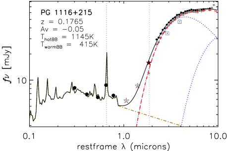
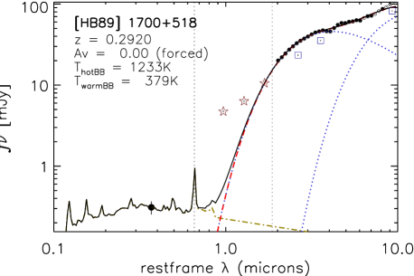
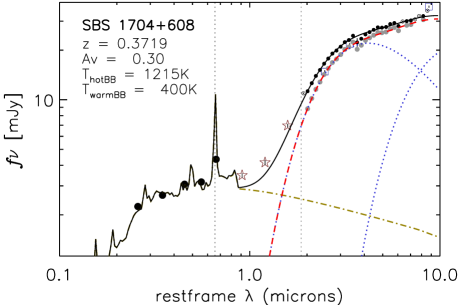
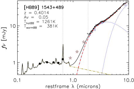
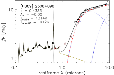
Figure 15: Spectral energy distributions of the sources in the sample. Circles, stars, and squares represent broadband photometry in the observed-frame optical (from SDSS), NIR (2MASS/UKIDSS/VHS), and MIR (WISE), respectively. Filled symbols indicate bands used to fit the disk component (yellow dot-dashed line). The (AKARI+)IRS spectra resampled at $\lambda$/$\Delta\lambda$ = 20 are shown with small black dots. Grey dots below the (AKARI+)IRS spectra represent the dust spectrum obtained after subtraction of the disk component. The model for the dust spectrum (red dashed line) is the linear combination of two black-bodies at adjustable temperatures (blue dotted lines). The combined disk+dust model is represented by the black solid line. The vertical dotted lines mark the restframe wavelength of the H$\alpha$ and Pa$\alpha$ recombination lines.

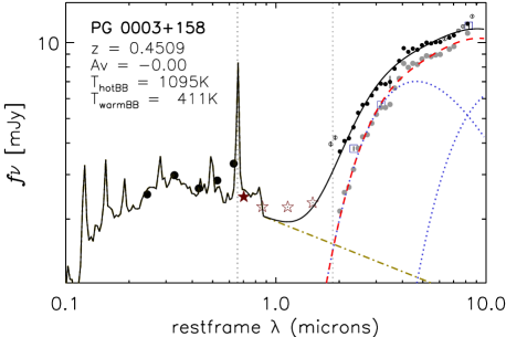
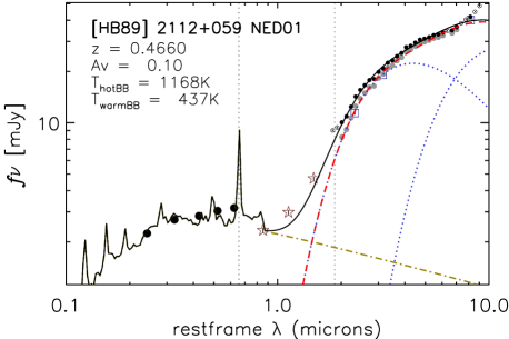
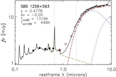
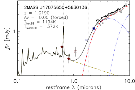
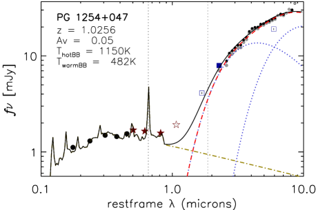
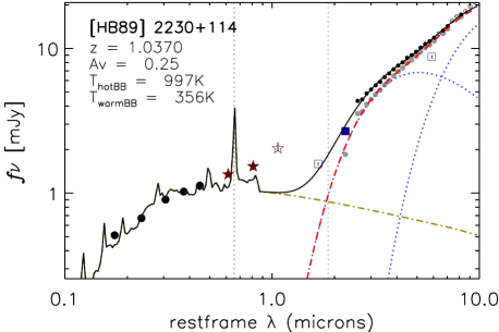
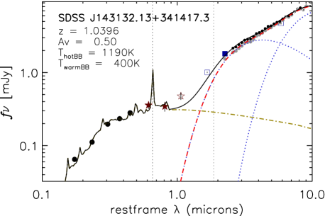
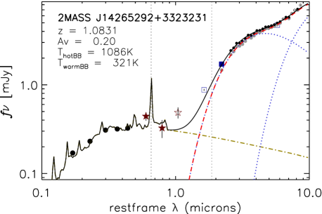
Figure 15: continued

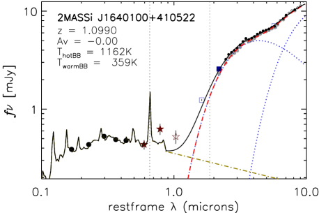
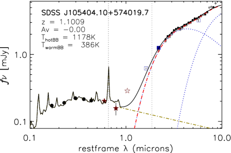
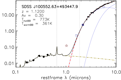
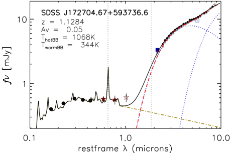
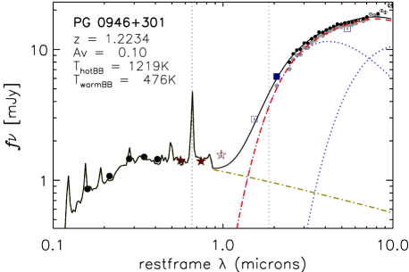
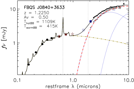
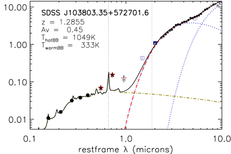
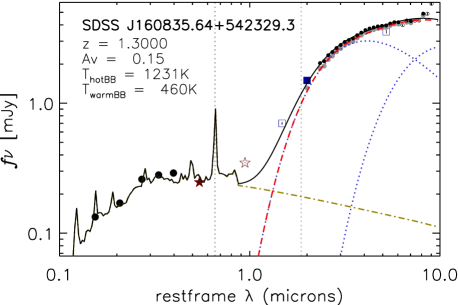
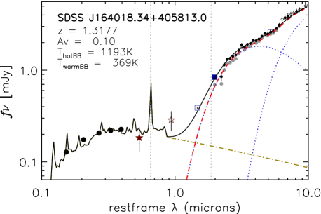
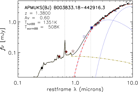
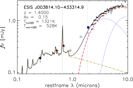
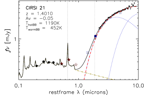
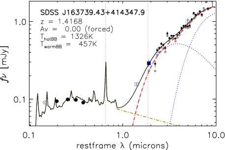
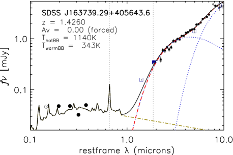
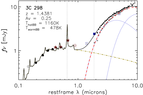
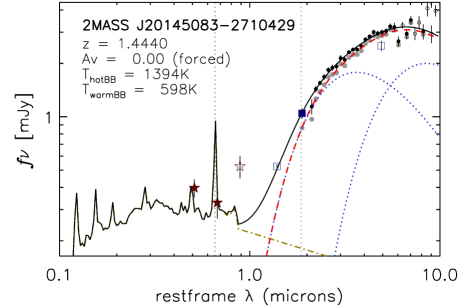
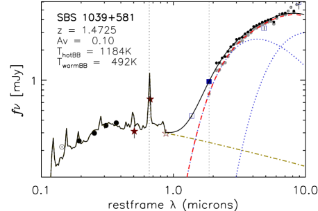
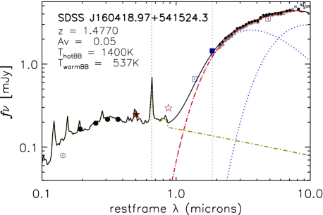
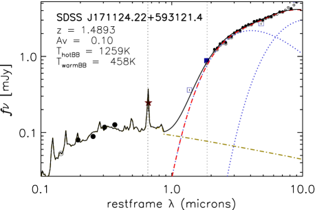
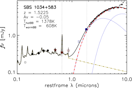
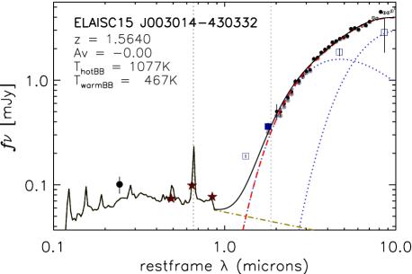
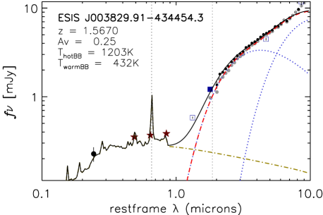
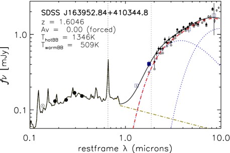
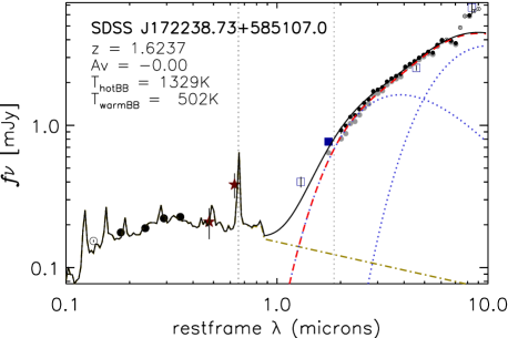
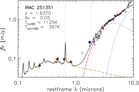
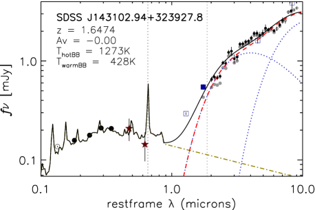
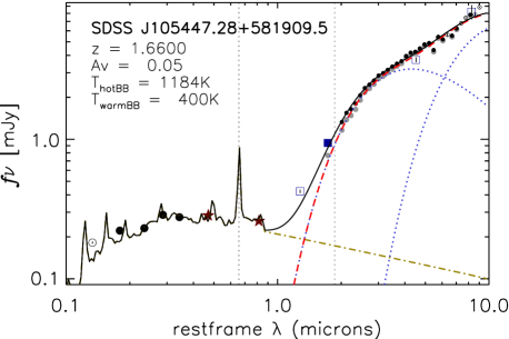
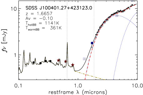
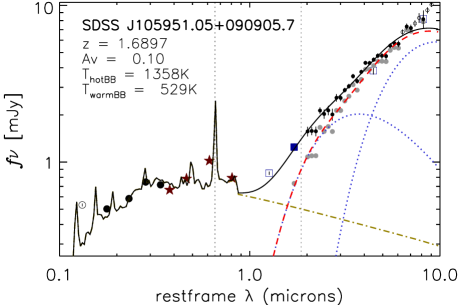
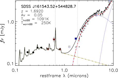
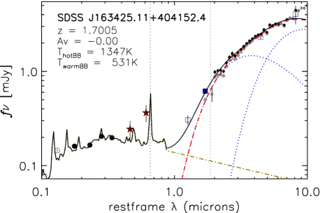
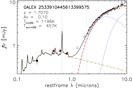
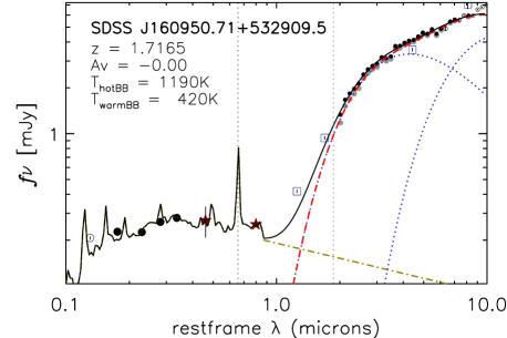
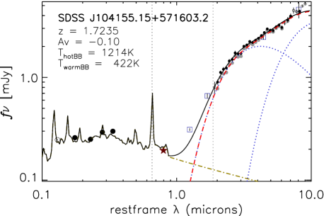
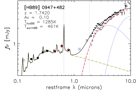
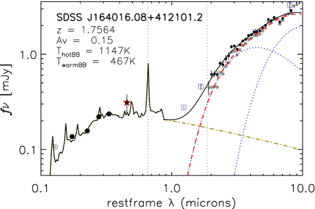
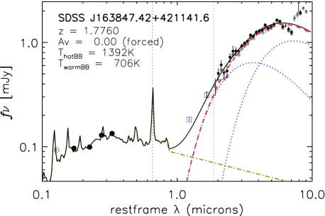
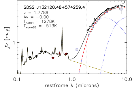
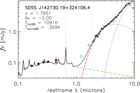
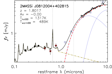
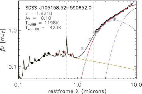
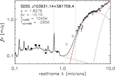
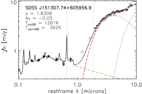
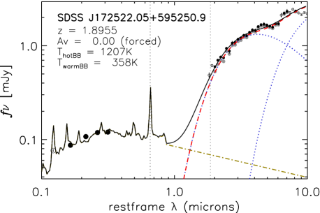
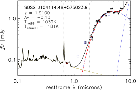
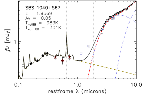
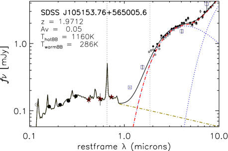
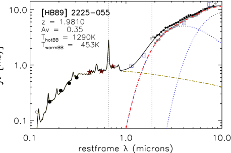
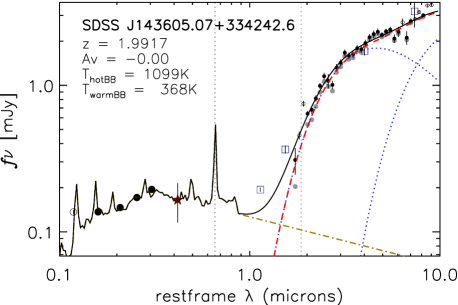
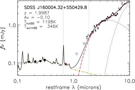
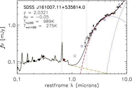
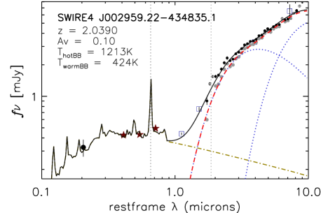
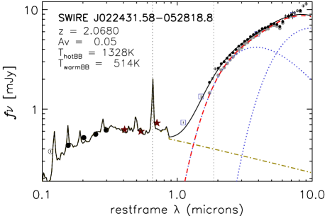
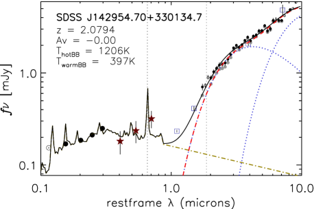
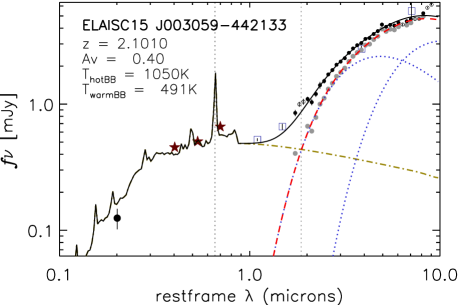
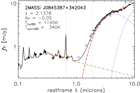
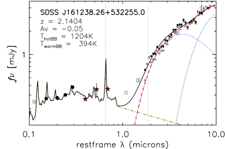
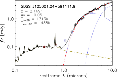
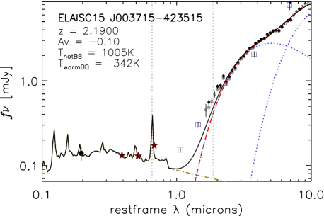
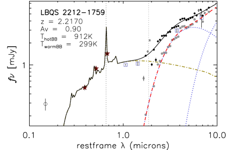
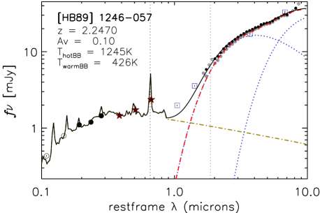
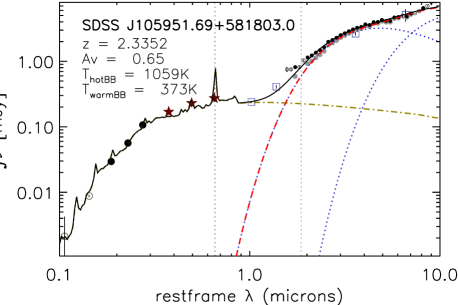
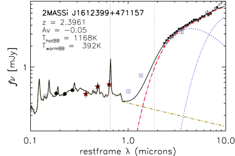
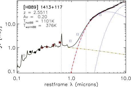
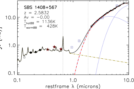
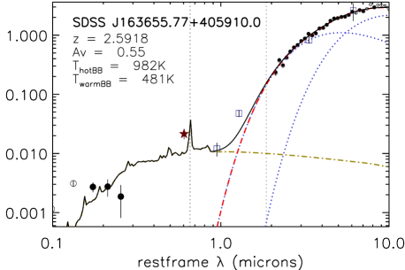
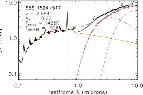
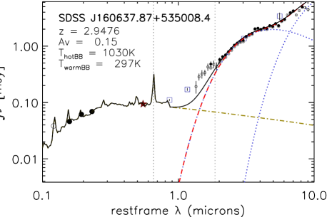
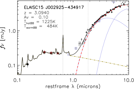
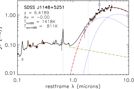
Figure 15: continued

Figure 15: continued

Figure 15: continued

Figure 15: continued

Figure 15: continued

Figure 15: continued

Figure 15: continued

Figure 15: continued

Figure 15: continued

References

- Alonso-Herrero et al. (2011) Alonso-Herrero A., et al., 2011, ApJ, 736, 82
- Antonucci (1993) Antonucci, R. 1993, ARA&A, 31, 473
- Barger et al. (2015) Barger A. J., Cowie L. L., Owen, F. N., Chen C.-C., Hasinger G., Hsu L.-Y., Li, Y., 2015, ApJ, 801, 87
- Barvainis (1987) Barvainis, R. 1987, ApJ 320, 537
- Bongiorno et al. (2012) Bongiorno, A., et al., 2012, MNRAS, 427, 3103
- Burtscher et al. (2015) Burtscher L., et al. 2015, A&A, 578, 47
- Clavel et al. (2006) Clavel J., Schartel N., Tomas L., 2006, A&A, 446, 439
- Cutri et al. (2012) Cutri R. M., et al. 2012, Explanatory Supplement to the WISE All-sky Data Release Products, http://adsabs.harvard.edu/abs/2012wise.rept….1C
- Deo et al. (2011) Deo, R. P., Richards, G. T., Nikutta, R., Elitzur, M., Gallagher, S. C., Ivezić, Z, Hines, D., 2011, ApJ, 729, 108
- Elvis et al. (1994) Elvis, M., Wilkes, B. J., McDowell, J. C. et al. 1994, ApJS, 95, 1
- Feltre et al. (2012) Feltre, A., Hatziminaoglou, E., Fritz, J., Franceschini, A. 2012, MNRAS, 426, 120
- Fritz et al. (2006) Fritz J., Franceschini A., Hatziminaoglou E. 2006, MNRAS, 366, 767
- Gallagher et al. (2007) Gallagher S. C., Richards G. T., Lacy M., Hines D. C., Elitzur, M., Storrie-Lombardi, L. J., 2007, ApJ, 661, 30
- Glikman et al. (2006) Glikman E., Helfand D. J., White R. L., 2006, ApJ, 640, 579
- Gordon et al. (2003) Gordon K. D., Clayton G. C., Misselt K. A., Landolt A. U. Wolff M. J., 2003, ApJ, 594, 279
- Granato & Danese (1994) Granato, G. L. and Danese, L., 1994, MNRAS, 268, 235
- Haas et al. (2003) Haas, M., Klaas, U., Müller, S. A. H., Bertoldi, F., Camenzind, M., et al. 2003, A&A, 402, 87
- Hao et al. (2010) Hao, H., et al., 2010, ApJL, 724, L59
- Hatziminaoglou et al. (2005) Hatziminaoglou, E., Pérez-Fournon, I., Polletta, M., Afonso-Luis, A., Hernán-Caballero, A., Montenegro-Montes, F. M. et al. 2005, AJ, 129, 1198
- Hernán-Caballero & Hatziminaoglou (2011) Hernán-Caballero A. & Hatziminaoglou E., 2011, MNRAS, 414, 500
- Hernán-Caballero et al. (2009) Hernán-Caballero A. et al., 2009, MNRAS, 395, 1695
- Hernán-Caballero et al. (2015) Hernán-Caballero A. et al., 2015, ApJ, 803, 109
- Hernán-Caballero et al. (2016) Hernán-Caballero, A., Spoon, H. W. W., Lebouteiller, V., Barry D. J., 2016, MNRAS, 455, 1796
- Hernán-Caballero (2012) Hernán-Caballero, A., 2012, MNRAS, 427, 816
- Hill et al. (2014) Hill, A. R., Gallagher, S. C., Deo, R. P., Peeters, E., Richards, G. T., 2014, MNRAS, 438, 2317
- Hönig et al. (2006) Hönig S. F., Beckert T., Ohnaka K., Weigelt G., 2006, A&A, 452, 459
- Hook et al. (1994) Hook I. M., McMahon R. G., Boyle B. J., Irwin M. J., 1994, MNRAS, 268, 305
- Hubeny et al. (2001) Hubeny I., Blaes O., Krolik J. H., Agol E., 2001, ApJ, 559, 680
- Kim et al. (2015) Kim, D., et al., 2015, ApJSS, 216, 17
- Kishimoto et al. (2008) Kishimoto, M., Antonucci, R., Blaes, O., et al. 2008, Nature, 454, 492
- Kozłowski (2016) Kozłowski S., 2016, ApJ in press (astro-ph/1604.05858)
- Krawczyk et al. (2015) Krawczyk, C. M., Richards, G. T., Gallagher, S. C., Leighly, K. M., Hewett, P. C., Ross, N. P., Hall, P. B., 2015, AJ, 149, 203
- Landt et al. (2008) Landt H., Padovani P., Giommi P., Perri M., Cheung C. C., 2008, ApJ, 676, 87
- Lawrence et al. (2007) Lawrence, A., Warren, S. J., Almaini, O. et al. 2007, MNRAS, 379, 15599
- Lebouteiller et al. (2011) Lebouteiller V., Barry D.J., Spoon H.W.W., Bernard-Salas J., Sloan G.C., Houck J.R., & Weedman D., 2011, ApJS, 196, 8
- Lebouteiller et al. (2015) Lebouteiller V., Barry, D. J., Goes, C., Sloan G. C., Spoon, H. W. W., Weedman, D. W., Bernard-Salas, J., Houck, J. R., 2015, ApJSS, 218, 21
- Lutz et al. (2008) Lutz D. et al., 2008, ApJ, 684, 853L
- Ma & Wang (2013) Ma X.-C., Wang T.-G., 2013, MNRAS, 430, 3445
- Maiolino et al. (2007) Maiolino R., Shemmer O., Imanishi M., Netzer H., Oliva E., Lutz D., Sturm E., 2007, A&A, 468, 979
- Markwardt (2009) Markwardt, C. B. 2009, Astronomical Data Analysis Software and Systems XVIII, 411, 251
- Mateos et al. (2015) Mateos, S. et al., 2015, MNRAS, 449, 1422
- Mateos et al. (2016) Mateos, S. et al., 2016, ApJ, 819, 166
- McMahon et al. (2013) McMahon R. G., Banerji M., Gonzalez E., Kopsov S. E., Béjar V. J., Lodieu N., Rebolo R., the VHS collaboration 2013, The Messenger, 154, 35
- Merloni (2015) Merloni A., 2015, in Haardt F., ed., Astrophysical Black Holes. Springer, International Publishing AG, Cham. preprint (arXiv:1505.04940)
- Meusinger & Weiss (2013) Meusinger H., Weiss V., 2013, A&A, 560, 140
- Mor et al. (2009) Mor R., Netzer H., Elitzur M., 2009, ApJ, 705, 298
- Nenkova et al. (2002) Nenkova M., Ivezic Z., Elitzur M., 2002, ApJ, 570, 9
- Nenkova et al. (2008) Nenkova M., Sirocky M.M., Ivezic Z., Elitzur M., 208, ApJ, 685, 147
- Netzer et al. (2007) Netzer H. et al., 2007, ApJ, 666, 806
- Netzer (2015) Netzer H., 2015, ARA&A, 53, 365
- Neugebauer et al. (1979) Neugebauer G. et al., 1979, ApJ, 230, 79
- Pâris et al. (2012) Pâris I. et al., 2012, A&A, 548, 66
- Rees et al. (1969) Rees M. J. et al., 1969, Nature, 223, 788
- Richards et al. (2001) Richards G. T. et al., 2001, AJ, 121, 2308
- Richards et al. (2006) Richards, G. T., et al., 2006, ApJS, 166, 470
- Rowan-Robinson (2000) Rowan-Robinson M., 2000, MNRAS, 316, 885
- Salpeter (1955) Salpeter E. E., 1955, ApJ, 121, 161
- Schlegel et al. (1998) Schlegel, D. J., Finkbeiner, D. P., and Davis, M. 1998, ApJ, 500, 525
- Schmidt & Hines (1999) Schmidt G. D., Hines D. C., 1999, ApJ, 512, 125
- Schneider et al. (2010) Schneider D. P., et al., 2010, AJ, 139, 2360
- Shakura & Sunyaev (1973) Shakura N. I., Sunyaev R. A., 1973, A&A, 24, 337
- Shen (2016) Shen Y., 2016, ApJ, 817, 55
- Siebenmorgen et al. (2015) Siebenmorgen R., Heymann F., Efstathiou A., 2015, A&A, 583, 120
- Skrutskie et al. (2006) Skrutskie, M. F., Cutri, R. M., Stiening, R. et al. 2006, AJ, 131, 1163
- Soifer et al. (2004) Soifer B. T. et al., 2004, ApJSS, 154, 151
- Stalevski et al. (2012) Stalevski M., Fritz J., Baes M., Nakos T., Popović L. C., 2012, MNRAS, 420, 2756
- Stalevski et al. (2016) Stalevski M., Ricci C., Ueda Y., Lira P., Fritz J., Baes M., 2016, MNRAS in press (astro-ph/1602.06954)
- Suganuma et al. (2006) Suganuma M., et al., 2006, ApJ, 639, 46
- Trump et al. (2006) Trump J. R. et al., 2006, ApJSS, 165, 1
- Vanden Berk et al. (2001) Vanden Berk, D. E., et al. 2001, AJ, 122, 549
- Veron & Veron (2006) Véron-Cetty M.P., Véron P., 2006, A&A, 455, 773
- Willott et al. (2003) Willott C. J., et al. 2003, MNRAS, 339, 397
- Wright et al. (2010) Wright E. L., et al., 2010, AJ, 140, 1868