h KA-TP-15-2016
Gauge-independent Renormalization of the
2-Higgs-Doublet Model

Abstract

The 2-Higgs-Doublet Model (2HDM) belongs to the simplest extensions of the Standard Model (SM) Higgs sector that are in accordance with theoretical and experimental constraints. In order to be able to properly investigate the experimental Higgs data and, in the long term to distinguish between possible models beyond the SM, precise predictions for the Higgs boson observables have to be made available on the theory side. This requires the inclusion of the higher order corrections. In this work, we investigate in detail the renormalization of the 2HDM, a pre-requisite for the computation of higher order corrections. We pay particular attention to the renormalization of the mixing angles $\alpha$ and $\beta$, which diagonalize the Higgs mass matrices and which enter all Higgs observables. The implications of various renormalization schemes in next-to-leading order corrections to the sample processes $H^{\pm}\to W^{\pm}h/H$ and $H\to ZZ$ are investigated. Based on our findings, we will present a renormalization scheme that is at the same time process independent, gauge independent and numerically stable.

1 Introduction

The discovery of a new scalar particle by the LHC experiments ATLAS [1] and CMS [2] in 2012 and its subsequent confirmation as being the Higgs boson [3, 4, 5, 6] marked a milestone for particle physics. At the same time, it triggered a change of paradigm. The Higgs particle, which formerly was the object of experimental searches, has itself become a tool in the search for New Physics (NP). Although the Standard Model (SM) of particle physics has been tested in previous and present experiments at the highest accuracy, there remain many open questions that cannot be answered within this model. The SM is therefore regarded as the low-energy description of some more fundamental theory that becomes effective at higher energy scales. A plethora of NP models have been discussed, among them e.g. supersymmetry (SUSY) as one of the most popular and most intensely studied Beyond the SM (BSM) extensions. Supersymmetry requires the introduction of at least two complex Higgs doublets. The Higgs sector of the Minimal Supersymmetric extension of the SM (MSSM) [7, 8, 9, 10] is a special case of the 2-Higgs-Doublet Model (2HDM) [7, 11, 12] type II. While the parameters of the SUSY Higgs potential are restricted due to SUSY relations, general 2HDMs allow for much more freedom in the choice of the parameters. They are therefore an ideal framework to study the implications of an extended Higgs sector for Higgs phenomenology at the LHC. This is reflected in the experimental analyses that interpret the results in various benchmark models, among them the 2HDM. The precise investigation of the Higgs sector aims at getting insights into the nature of electroweak symmetry breaking (EWSB) and at clarifying the question whether it is based on weakly or strongly interacting dynamics. Deviations in the properties of the discovered SM-like Higgs boson are hints towards NP. In particular, the higher precision in the Higgs couplings measurements at the LHC run 2 and in the high-luminosity option allows to search indirectly for BSM effects. This becomes increasingly important in view of the null results of direct searches for NP so far. The precise measurements on the experimental side, however, call for precise predictions of parameters and observables from theory. Accurate theory predictions are indispensable not only for the proper interpretation of the experimental data, but also for the correct determination of the parameter space that is still allowed in the various models, and, finally, for the distinction between different BSM extensions.

With this paper we contribute to the effort of providing precise predictions for parameters and observables relevant for the phenomenology at the LHC and future $e^{+}e^{-}$ colliders. We investigate higher order corrections in the framework of the 2HDM. While 2HDMs are interesting because they contain the MSSM Higgs sector as a special case, they also belong to the simplest SM extensions respecting basic experimental and theoretical constraints that are testable at the LHC. After EWSB they feature five physical Higgs bosons, two neutral CP-even, one neutral CP-odd and two charged Higgs bosons. They represent an ideal benchmark framework to investigate the various possible NP effects to be expected at the LHC in multi-Higgs boson sectors. Finally, specific 2HDM versions also allow for a Dark Matter (DM) candidate [15, 16, 17, 18, 19, 20, 21]. In the past, numerous papers have provided higher order corrections to the 2HDM parameters, production cross sections and decay widths. Several papers have dealt with the renormalization of the 2HDM (see e.g. [22, 23, 24]). In particular, the renormalization of the mixing angles $\alpha$ and $\beta$ is of interest. While $\alpha$ is introduced to diagonalize the mass matrix of the neutral CP-even Higgs sector, the angle $\beta$ appears in the diagonalization of the CP-odd and the charged Higgs sector, respectively. These angles define the Higgs couplings to the SM particles and thus enter all Higgs observables like e.g. production cross sections and decay widths. For the MSSM it was stated in [25] that a renormalization scheme for the only mixing angle taken as an independent parameter from the scalar sector, $\beta$, cannot be simultaneously gauge independent, process independent and numerically stable. In the 2HDM also $\alpha$ needs to be renormalized, which has important consequences for the choice of the renormalization scheme. If the tadpoles are treated in the usual way, which we call the standard approach (cf. 3.1.1), a process-independent definition of the angular counterterms is prone to lead to gauge-dependent amplitudes and consequently to gauge-dependent physical observables. This is the case e.g. in the scheme presented in [23]. There are essentially two possibilities to circumvent the emergence of this gauge dependence. Either one gives up the requirement of process independence and fixes $\alpha$ and $\beta$ in terms of a physical observable or one changes the treatment of the tadpoles. As we will see, this will decouple the issue of gauge dependence from the definition of $\delta\alpha$ and $\delta\beta$ and allow for process- and gauge-independent angular counterterms leading to manifestly gauge-independent amplitudes.

In this paper we study in detail the renormalization of the 2HDM Higgs sector with the main focus on the investigation of the gauge dependence of the renormalization of the mixings angles $\alpha$ and $\beta$. We propose several schemes and compare them both to the ones in the literature and amongst each other. In sample decay processes we investigate the numerical differences and in particular the numerical stability of the various renormalization prescriptions. Our results presented here will serve as basis for the further computation of the one-loop electroweak corrections to all 2HDM Higgs boson decays.

The organization of the paper is as follows. In sec. 2 we introduce the model and set up our notation. The following sec. 3 is devoted to the detailed presentation and discussion of the various renormalization prescriptions that will be applied. Section 4 deals with the computation of the electroweak (EW) one-loop corrections to various decay processes and the discussion of the gauge dependence of the angular counterterms. In sec. 5 we present our numerical results. We finish with the conclusions in sec. 6. The paper is accompanied by an extensive Appendix to serve as starting point for further investigations of the 2HDM renormalization.

2 Description of the Model

We work in the framework of a general 2HDM with a global discrete $\mathbb{Z}_{2}$ symmetry that is softly broken. The kinetic term of the two $SU(2)$ Higgs doublets $\Phi_{1}$ and $\Phi_{2}$ is given by

$${\cal L}_{\text{kin}}=\sum_{i=1}^{2}(D_{\mu}\Phi_{i})^{\dagger}(D^{\mu}\Phi_{i})$$ (2.1)

in terms of the covariant derivative

$$D_{\mu}=\partial_{\mu}+\frac{i}{2}g\sum_{a=1}^{3}\tau^{a}W_{\mu}^{a}+\frac{i}{2}g^{\prime}B_{\mu}\;,$$ (2.2)

where $\tau^{a}$ denote the Pauli matrices, $W_{\mu}^{a}$ and $B_{\mu}$ the $SU(2)_{L}$ and $U(1)_{Y}$ gauge bosons, respectively, and $g$ and $g^{\prime}$ the corresponding gauge couplings. The scalar potential that can be built from the two $SU(2)$ Higgs doublets can be written as

$$V = m_{11}^{2}|\Phi_{1}|^{2}+m_{22}^{2}|\Phi_{2}|^{2}-m_{12}^{2}(\Phi_{1}^{\dagger}\Phi_{2}+h.c.)+\frac{\lambda_{1}}{2}(\Phi_{1}^{\dagger}\Phi_{1})^{2}+\frac{\lambda_{2}}{2}(\Phi_{2}^{\dagger}\Phi_{2})^{2}$$ (2.3)

$$+\lambda_{3}(\Phi_{1}^{\dagger}\Phi_{1})(\Phi_{2}^{\dagger}\Phi_{2})+\lambda_{4}(\Phi_{1}^{\dagger}\Phi_{2})(\Phi_{2}^{\dagger}\Phi_{1})+\frac{\lambda_{5}}{2}[(\Phi_{1}^{\dagger}\Phi_{2})^{2}+h.c.]\;.$$

The discrete $\mathbb{Z}_{2}$ symmetry ($\Phi_{1}\to-\Phi_{1},\Phi_{2}\to\Phi_{2}$) ensures the absence of tree-level Flavour Changing Neutral Currents. Assuming CP conservation, the 2HDM potential depends on eight real parameters, three mass parameters, $m_{11}$, $m_{22}$ and $m_{12}$, and five coupling parameters $\lambda_{1}$-$\lambda_{5}$. Through the term proportional to $m_{12}^{2}$ the discrete $\mathbb{Z}_{2}$ symmetry is softly broken. After EWSB the neutral components of the Higgs doublets develop vacuum expectation values (VEVs), which are real in the CP-conserving case. Expanding about the VEVs $v_{1}$ and $v_{2}$ and expressing each doublet $\Phi_{i}$ $(i=1,2)$ in terms of the charged complex field $\phi_{i}^{+}$ and the real neutral CP-even and CP-odd fields $\rho_{i}$ and $\eta_{i}$, respectively,

$$\Phi_{1}=\left(\begin{array}[]{c}\phi_{1}^{+}\\ \frac{\rho_{1}+i\eta_{1}+v_{1}}{\sqrt{2}}\end{array}\right)\qquad\mbox{and}\qquad\Phi_{2}=\left(\begin{array}[]{c}\phi_{2}^{+}\\ \frac{\rho_{2}+i\eta_{2}+v_{2}}{\sqrt{2}}\end{array}\right)\;,$$ (2.8)

leads to the mass matrices, which are obtained from the terms bilinear in the Higgs fields in the potential. Due to charge and CP conservation they decompose into $2\times 2$ matrices ${\cal M}_{S}$, ${\cal M}_{P}$ and ${\cal M}_{C}$ for the neutral CP-even, neutral CP-odd and charged Higgs sector. They are diagonalized by the following orthogonal transformations

$$\left(\begin{array}[]{c}\rho_{1}\\ \rho_{2}\end{array}\right) = R(\alpha)\left(\begin{array}[]{c}H\\ h\end{array}\right)\;,$$ (2.13)

$$\left(\begin{array}[]{c}\eta_{1}\\ \eta_{2}\end{array}\right) = R(\beta)\left(\begin{array}[]{c}G^{0}\\ A\end{array}\right)\;,$$ (2.18)

$$\left(\begin{array}[]{c}\phi_{1}^{\pm}\\ \phi^{\pm}_{2}\end{array}\right) = R(\beta)\left(\begin{array}[]{c}G^{\pm}\\ H^{\pm}\end{array}\right)\;,$$ (2.23)

leading to the physical Higgs states, a neutral light CP-even, $h$, a neutral heavy CP-even, $H$, a neutral CP-odd, $A$, and two charged Higgs bosons, $H^{\pm}$. The massless pseudo-Nambu-Goldstone bosons $G^{\pm}$ and $G^{0}$ are absorbed by the longitudinal components of the massive gauge bosons, the charged $W^{\pm}$ and the $Z$ boson, respectively. The rotation matrices in terms of the mixing angles $\vartheta=\alpha$ and $\beta$, respectively, read

$$R(\vartheta)=\left(\begin{array}[]{cc}\cos\vartheta&-\sin\vartheta\\ \sin\vartheta&\cos\vartheta\end{array}\right)\;.$$ (2.26)

The mixing angle $\beta$ is related to the two VEVs as

$$\tan\beta=\frac{v_{2}}{v_{1}}\;,$$ (2.27)

with $v_{1}^{2}+v_{2}^{2}=v^{2}\approx(246\mbox{ GeV})^{2}$, while the mixing angle $\alpha$ is expressed through

$$\tan 2\alpha=\frac{2({\cal M}_{S})_{12}}{({\cal M}_{S})_{11}-({\cal M}_{S})_{22}}\;,$$ (2.28)

where $({\cal M}_{S})_{ij}$ ($i,j=1,2$) denote the matrix elements of the neutral CP-even scalar mass matrix ${\cal M}_{S}$. With

$$M^{2}\equiv\frac{m_{12}^{2}}{s_{\beta}c_{\beta}}$$ (2.29)

we have [23]

$$\tan 2\alpha=\frac{s_{2\beta}(M^{2}-\lambda_{345}v^{2})}{c_{\beta}^{2}(M^{2}-\lambda_{1}v^{2})-s_{\beta}^{2}(M^{2}-\lambda_{2}v^{2})}\;,$$ (2.30)

where we have introduced the abbreviation

$$\lambda_{345}\equiv\lambda_{3}+\lambda_{4}+\lambda_{5}$$ (2.31)

and used short-hand notation $s_{x}\equiv\sin x$ etc.

The minimization conditions of the Higgs potential require the terms linear in the Higgs fields to vanish in the vacuum, i.e.

$$\left\langle\frac{\partial V}{\partial\Phi_{1}}\right\rangle=\left\langle\frac{\partial V}{\partial\Phi_{2}}\right\rangle=0\;,$$ (2.32)

where the brackets denote the vacuum. The corresponding coefficients, the tadpole parameters $T_{1}$ and $T_{2}$, therefore have to be zero. The tadpole conditions at lowest order are given by

$$\left\langle\frac{\partial V}{\partial\Phi_{1}}\right\rangle \equiv \frac{T_{1}}{v_{1}}=m_{11}^{2}-m_{12}^{2}\frac{v_{2}}{v_{1}}+\frac{\lambda_{1}v_{1}^{2}}{2}+\frac{\lambda_{345}v_{2}^{2}}{2}$$ (2.33)

$$\left\langle\frac{\partial V}{\partial\Phi_{2}}\right\rangle \equiv \frac{T_{2}}{v_{2}}=m_{22}^{2}-m_{12}^{2}\frac{v_{1}}{v_{2}}+\frac{\lambda_{2}v_{2}^{2}}{2}+\frac{\lambda_{345}v_{1}^{2}}{2}\;.$$ (2.34)

There are various possibilities to choose the set of independent parameters that parametrizes the Higgs potential $V$. Thus, Eqs. (2.33) and (2.34) can be used to replace $m_{11}^{2}$ and $m_{22}^{2}$ by the tadpole parameters $T_{1}$ and $T_{2}$. The VEV $v$ can furthermore be expressed in terms of the physical gauge boson masses $M_{W}$ and $M_{Z}$ and the electric charge $e$. In the following, we will choose the set of independent parameters such that the parameters can be related to as many physical quantities as possible. Our set is given by the Higgs boson masses, the tadpole parameters, the two mixing angles, the soft breaking parameter, the massive gauge boson masses and the electric charge. Additionally, we will need the fermion masses $m_{f}$ for the Higgs decays into fermions which will be used for a process-dependent definition of the angular counterterms.

$$\mbox{\text@underline{Input parameters:}}\quad m_{h},\;m_{H},\;m_{A},\;m_{H^{\pm}},\;T_{1},\;T_{2},\;\alpha,\;\tan\beta,\;m_{12}^{2},\;M_{W}^{2},\;M_{Z}^{2},\;e,\;m_{f}\;.$$ (2.35)

3 Renormalization

In this section we will present the various renormalization schemes that we will apply in the renormalization of the 2HDM and that will be investigated with respect to their gauge parameter dependence and their numerical stability. We will use these schemes in sample processes given by the EW one-loop corrected decays of the charged Higgs boson into a $W^{\pm}$ and a CP-even Higgs boson, $H^{\pm}\to W^{\pm}h/H$, and of the heavy $H$ into a $Z$ boson pair, $H\to ZZ$. The computation of the EW one-loop corrections leads to ultraviolet (UV) divergences. In the charged Higgs decay we will furthermore encounter infrared (IR) divergences because of massless photons running in the loops. The UV divergences in the virtual corrections are canceled by the renormalization of the parameters involved in the EW corrections of the process, while the IR ones are subtracted by taking into account the real corrections. The renormalization of the above decay processes requires the renormalization of the electroweak sector and of the Higgs sector. We will also compute the EW one-loop corrections to the decays of $H$ and $A$ into $\tau$ leptons, $H/A\to\tau\tau$. These processes will be exploited for a process-dependent definition of the angular counterterms, which will be presented as a possible renormalization scheme among others. The corrections to the decays into $\tau$ leptons also require the renormalization of the fermion sector. Note, that the renormalization of the CKM matrix, which we will assume to be real, will not play a role in our renormalization procedure. We start by replacing the relevant parameters by the renormalized ones and their corresponding counterterms:

Gauge sector: The massive gauge boson masses and the electric charge are replaced by

$$M_{W}^{2} \to M_{W}^{2}+\delta M_{W}^{2}$$ (3.1)

$$M_{Z}^{2} \to M_{Z}^{2}+\delta M_{Z}^{2}$$ (3.2)

$$e \to (1+\delta Z_{e})\,e\;.$$ (3.3)

Equally, the VEV $v$, which will be expressed in terms of these parameters, is replaced by

$$v \to v+\delta v\;.$$ (3.4)

The gauge boson fields are renormalized by their field renormalization constants $\delta Z$,

$$W^{\pm} \to \left(1+\frac{1}{2}\delta Z_{WW}\right)W^{\pm}$$ (3.5)

$$\left(\begin{array}[]{c}Z\\ \gamma\end{array}\right) \to \left(\begin{array}[]{cc}1+\frac{1}{2}\delta Z_{ZZ}&\frac{1}{2}\delta Z_{Z\gamma}\\ \frac{1}{2}\delta Z_{\gamma Z}&1+\frac{1}{2}\delta Z_{\gamma\gamma}\end{array}\right)\left(\begin{array}[]{c}Z\\ \gamma\end{array}\right)\;.$$ (3.12)

Fermion sector: The counterterms to the fermion masses $m_{f}$ are defined through

$$m_{f}\to m_{f}+\delta m_{f}\;.$$ (3.13)

The bare left- and right-handed fermion fields

$$f_{L/R}\equiv P_{L/R}f\quad\;,\quad\mbox{ with }\quad P_{L/R}=(1\mp\gamma_{5})/2\;,$$ (3.14)

are replaced by their corresponding renormalized fields according to

$$f_{L/R}\to\left(1+\frac{1}{2}\delta Z^{L/R}_{f}\right)f_{L/R}\;.$$ (3.15)

Higgs sector: The renormalization is performed in the mass basis and the mass counterterms are defined through

$$m_{h}^{2} \to m_{h}^{2}+\delta m_{h}^{2}$$ (3.16)

$$m_{H}^{2} \to m_{H}^{2}+\delta m_{H}^{2}$$ (3.17)

$$m_{A}^{2} \to m_{A}^{2}+\delta m_{A}^{2}$$ (3.18)

$$m_{H^{\pm}}^{2} \to m_{H^{\pm}}^{2}+\delta m_{H^{\pm}}^{2}\;.$$ (3.19)

The fields are replaced by the renormalized ones and the field renormalization constants as

$$\left(\begin{array}[]{c}H\\ h\end{array}\right) \to \left(\begin{array}[]{cc}1+\frac{1}{2}\delta Z_{HH}&\frac{1}{2}\delta Z_{Hh}\\ \frac{1}{2}\delta Z_{hH}&1+\frac{1}{2}\delta Z_{hh}\end{array}\right)\left(\begin{array}[]{c}H\\ h\end{array}\right)$$ (3.26)

$$\left(\begin{array}[]{c}G^{0}\\ A\end{array}\right) \to \left(\begin{array}[]{cc}1+\frac{1}{2}\delta Z_{G^{0}G^{0}}&\frac{1}{2}\delta Z_{G^{0}A}\\ \frac{1}{2}\delta Z_{AG^{0}}&1+\frac{1}{2}\delta Z_{AA}\end{array}\right)\left(\begin{array}[]{c}G^{0}\\ A\end{array}\right)$$ (3.33)

$$\left(\begin{array}[]{c}G^{\pm}\\ H^{\pm}\end{array}\right) \to \left(\begin{array}[]{cc}1+\frac{1}{2}\delta Z_{G^{\pm}G^{\pm}}&\frac{1}{2}\delta Z_{G^{\pm}H^{\pm}}\\ \frac{1}{2}\delta Z_{H^{\pm}G^{\pm}}&1+\frac{1}{2}\delta Z_{H^{\pm}H^{\pm}}\end{array}\right)\left(\begin{array}[]{c}G^{\pm}\\ H^{\pm}\end{array}\right)$$ (3.40)

and the mixing angles by

$$\alpha \to \alpha+\delta\alpha$$ (3.41)

$$\beta \to \beta+\delta\beta\;.$$ (3.42)

While the tadpoles vanish at leading order, the terms linear in the Higgs fields get loop contributions at higher orders. Therefore, also the tadpole parameters $T_{1}$ and $T_{2}$ have to be renormalized in order to fulfill the tadpole conditions Eqs. (2.32). The tadpoles are hence replaced as

$$T_{1}\to T_{1}+\delta T_{1}\qquad\mbox{and}\qquad T_{2}\to T_{2}+\delta T_{2}\;.$$ (3.43)

3.1 Renormalization conditions

The finite parts of the counterterms are fixed by the renormalization conditions. Throughout we will fix the renormalization constants for the masses and fields through on-shell (OS) conditions. The renormalization schemes differ, however, in the treatment of the tadpoles and of the mixing angles. We will describe two different approaches for the treatment of the tadpoles. Both of them apply the same renormalization conditions for the tadpoles. They differ, however, in the way the minimum conditions are applied when the mass counterterms are generated. As a consequence, the tadpole counterterms can either explicitly show up in the mass counterterms or not. The latter case, that we will call ’alternative tadpole’ or in short ’tadpole’ scheme, has the virtue that the mass counterterms are manifestly gauge independent, while in the former one, named ’standard tadpole’ or simply ’standard’ scheme, this is not the case. The authors of Ref. [23] have combined the standard tadpole scheme with the definition of the counterterms through off-diagonal wave function renormalization constants. This ’KOSY’ scheme, denoted by the initials of the authors, leads to manifestly gauge-dependent decay amplitudes, as we will show. In the alternative tadpole scheme not only this problem does not occur, but in addition, the angular counterterms are explicitly gauge independent. If the angular counterterms are defined in a ’process-dependent’ scheme via a physical process, the decay amplitude is gauge independent irrespective of the treatment of the tadpoles. The only difference lies in the gauge independence of the angular counterterms in case the alternative tadpole scheme is adopted. In the following, the renormalization conditions of the various schemes will be introduced.

3.1.1 Standard Tadpole Scheme

We start by presenting the usual, i.e. ’standard’, approach in the renormalization of the 2HDM as also applied in [23, 24]. The gauge bosons are renormalized through OS conditions, which implies the following counterterms for the masses,

$$\delta M_{W}^{2}=\mbox{Re}\,\Sigma^{T}_{WW}(M_{W}^{2})\quad\mbox{and}\quad\delta M_{Z}^{2}=\mbox{Re}\,\Sigma^{T}_{ZZ}(M_{Z}^{2})\;,$$ (3.44)

where the superscript $T$ denotes the transverse part of the respective self-energy $\Sigma$. In order to guarantee the correct OS properties the wave function renormalization constants have to be introduced as

$$\delta Z_{WW} = -\mbox{Re}\left.\frac{\partial\Sigma^{T}_{WW}(p^{2})}{\partial p^{2}}\right|_{p^{2}=M_{W}^{2}}$$ (3.45)

$$\left(\begin{array}[]{cc}\delta Z_{ZZ}&\delta Z_{Z\gamma}\\ \delta Z_{\gamma Z}&\delta Z_{\gamma\gamma}\end{array}\right) = \left(\begin{array}[]{cc}-\mbox{Re}\left.\frac{\partial\Sigma^{T}_{ZZ}(p^{2})}{\partial p^{2}}\right|_{p^{2}=M_{Z}^{2}}&2\frac{\Sigma^{T}_{Z\gamma}(0)}{M_{Z}^{2}}\\ -2\mbox{Re}\frac{\Sigma^{T}_{Z\gamma}(M_{Z}^{2})}{M_{Z}^{2}}&-\left.\frac{\partial\Sigma^{T}_{\gamma\gamma}(p^{2})}{\partial p^{2}}\right|_{p^{2}=0}\end{array}\right)\;.$$ (3.50)

The electric charge is defined to be the full electron-positron photon coupling for OS external particles in the Thomson limit, implying that all corrections to this vertex vanish OS and for zero momentum transfer. The counterterm for the electric charge in terms of the transverse photon-photon and photon-$Z$ self-energies reads [26]

$$\delta Z_{e}^{\alpha(0)} = \frac{1}{2}\left.\frac{\partial\Sigma^{T}_{\gamma\gamma}(k^{2})}{\partial k^{2}}\right|_{k^{2}=0}+\frac{s_{W}}{c_{W}}\frac{\Sigma_{\gamma Z}^{T}(0)}{M_{Z}^{2}}\;,$$ (3.51)

where $s_{W}/c_{W}\equiv\sin\theta_{W}/\cos\theta_{W}$ and $\theta_{W}$ denotes the Weinberg angle. Note that the sign in the second term of Eq. (3.51) differs from the one in [26] due to our sign conventions in the covariant derivative of Eq. (2.2). In our computation, however, we will use the fine structure constant at the $Z$ boson mass $\alpha(M_{Z}^{2})$ as input, so that the results are independent of large logarithms due to light fermions $f\neq t$. The counterterm $\delta Z_{e}$ is therefore modified as [26]

$$\delta Z_{e}^{\alpha(M_{Z}^{2})} = \delta Z_{e}^{\alpha(0)}-\frac{1}{2}\Delta\alpha(M_{Z}^{2})$$ (3.52)

$$\Delta\alpha(M_{Z}^{2}) = \left.\frac{\partial\Sigma^{T}_{\gamma\gamma}(k^{2})}{\partial k^{2}}\right|_{k^{2}=0}-\frac{\Sigma^{T}_{\gamma\gamma}(M_{Z}^{2})}{M_{Z}^{2}}\;,$$ (3.53)

where the transverse part of the photon self-energy $\Sigma^{T}_{\gamma\gamma}$ in Eq. (3.53) includes only the light fermion contributions. For the computation of the EW one-loop corrected Higgs decay widths we also need to renormalize the coupling $g$, which can be related to $e$ and the gauge boson masses as

$$g = \frac{eM_{Z}}{\sqrt{M_{Z}^{2}-M_{W}^{2}}}\;,$$ (3.54)

so that its counterterm can be expressed in terms of the gauge boson mass counterterms through

$$\frac{\delta g}{g}=\delta Z_{e}-\frac{1}{2(1-M_{Z}^{2}/M_{W}^{2})}\left(\frac{\delta M_{W}^{2}}{M_{W}^{2}}-\frac{\delta M_{Z}^{2}}{M_{Z}^{2}}\right)\;.$$ (3.55)

Defining the following structure for the fermion self-energies

$$\Sigma_{f}(p^{2})=/{\!\!\!p}\Sigma^{L}_{f}(p^{2})P_{L}+/{\!\!\!p}\Sigma^{R}_{f}(p^{2})P_{R}+m_{f}\Sigma^{Ls}_{f}(p^{2})P_{L}+m_{f}\Sigma^{Rs}_{f}(p^{2})P_{R}$$ (3.56)

the fermion mass counterterms applying OS conditions are given by

$$\frac{\delta m_{f}}{m_{f}}=\frac{1}{2}\mbox{Re}\left[\Sigma^{L}_{f}(m_{f}^{2})+\Sigma^{R}_{f}(m_{f}^{2})+\Sigma^{Ls}_{f}(m_{f}^{2})+\Sigma^{Rs}_{f}(m_{f}^{2})\right]\;.$$ (3.57)

The fermion wave function renormalization constants are determined from

$$\delta Z^{L/R}_{f} = -\mbox{Re}\Sigma^{L/R}_{f}(m_{f}^{2})$$ (3.58)

$$-m_{f}^{2}\frac{\partial}{\partial p^{2}}\mbox{Re}\left.\left(\Sigma^{L/R}_{f}(p^{2})+\Sigma^{R/L}_{f}(p^{2})+\Sigma^{L/Rs}_{f}(p^{2})+\Sigma^{R/Ls}_{f}(p^{2})\right)\right|_{p^{2}=m_{f}^{2}}\,.$$

The OS conditions for the physical Higgs bosons yield the following Higgs mass counterterms

$$\delta m_{H}^{2} = \mbox{Re}[\Sigma_{HH}(m_{H}^{2})-\delta T_{HH}]\;,\qquad\delta m_{h}^{2}=\mbox{Re}[\Sigma_{hh}(m_{h}^{2})-\delta T_{hh}]\;,$$ (3.59)

$$\delta m_{A}^{2} = \mbox{Re}[\Sigma_{AA}(m_{A}^{2})-\delta T_{AA}]\;,\qquad\delta m_{H^{\pm}}^{2}=\mbox{Re}[\Sigma_{H^{\pm}H^{\pm}}(m_{H^{\pm}}^{2})-\delta T_{H^{\pm}H^{\pm}}]\;.$$ (3.60)

The appearance of the tadpole counterterms in Eqs. (3.59) and (3.60) can be understood by recalling that the parameters $m_{11}^{2}$ and $m_{22}^{2}$, which enter the mass matrices, can be replaced by the tadpole coefficients $T_{1}$ and $T_{2}$. Applying the shifts Eq. (3.43) and rotating into the mass eigenbasis yield the above conditions in the OS scheme. The relations between the tadpole counterterms in the mass basis and $\delta T_{1,2}$ are given by

$$\delta T_{HH} = \frac{\delta T_{1}}{v_{1}}\cos^{2}\vartheta+\frac{\delta T_{2}}{v_{2}}\sin^{2}\vartheta\;,$$ (3.61)

$$\delta T_{hh/AA/H^{\pm}H^{\pm}} = \frac{\delta T_{1}}{v_{1}}\sin^{2}\vartheta+\frac{\delta T_{2}}{v_{2}}\cos^{2}\vartheta\;,$$ (3.62)

$$\mbox{with }\vartheta = \left\{\begin{array}[]{cll}\alpha&\mbox{ for }&\delta T_{HH,hh}\\ \beta&\mbox{ for }&\delta T_{AA,H^{\pm}H^{\pm}}\end{array}\right.\;.$$ (3.65)

The tadpoles are renormalized such that the correct vacuum is reproduced at one-loop order, leading to the renormalization conditions

$$\delta T_{1}=T_{1}\qquad\mbox{and}\qquad\delta T_{2}=T_{2}\;.$$ (3.66)

The $T_{1,2}$ stand for the contributions coming from the corresponding genuine Higgs boson tadpole graphs in the gauge basis. For the wave function renormalization constants the OS renormalization implies the following conditions

$$\left(\begin{array}[]{cc}\delta Z_{HH}&\delta Z_{Hh}\\ \delta Z_{hH}&\delta Z_{hh}\end{array}\right) = \left(\begin{array}[]{cc}-\mbox{Re}\left.\frac{\partial\Sigma_{HH}(k^{2})}{\partial k^{2}}\right|_{k^{2}=m_{H}^{2}}&2\frac{\mbox{Re}\left[\Sigma_{Hh}(m_{h}^{2})-\delta T_{Hh}\right]}{m_{H}^{2}-m_{h}^{2}}\\[8.5359pt] -2\frac{\mbox{Re}\left[\Sigma_{Hh}(m_{H}^{2})-\delta T_{Hh}\right]}{m_{H}^{2}-m_{h}^{2}}&-\mbox{Re}\left.\frac{\partial\Sigma_{hh}(k^{2})}{\partial k^{2}}\right|_{k^{2}=m_{h}^{2}}\end{array}\right)$$ (3.71)

$$\left(\begin{array}[]{cc}\delta Z_{G^{0}G^{0}}&\delta Z_{G^{0}A}\\ \delta Z_{AG^{0}}&\delta Z_{AA}\end{array}\right) = \left(\begin{array}[]{cc}-\mbox{Re}\left.\frac{\partial\Sigma_{G^{0}G^{0}}(k^{2})}{\partial k^{2}}\right|_{k^{2}=0}&-2\frac{\mbox{Re}\left[\Sigma_{G^{0}A}(m_{A}^{2})-\delta T_{G^{0}A}\right]}{m_{A}^{2}}\\[8.5359pt] 2\frac{\mbox{Re}\left[\Sigma_{G^{0}A}(0)-\delta T_{G^{0}A}\right]}{m_{A}^{2}}&-\mbox{Re}\left.\frac{\partial\Sigma_{AA}(k^{2})}{\partial k^{2}}\right|_{k^{2}=m_{A}^{2}}\end{array}\right)$$ (3.76)

$$\left(\begin{array}[]{cc}\delta Z_{G^{\pm}G^{\pm}}&\delta Z_{G^{\pm}H^{\pm}}\\ \delta Z_{H^{\pm}G^{\pm}}&\delta Z_{H^{\pm}H^{\pm}}\end{array}\right) = \left(\begin{array}[]{cc}-\mbox{Re}\left.\frac{\partial\Sigma_{G^{\pm}G^{\pm}}(k^{2})}{\partial k^{2}}\right|_{k^{2}=0}&-2\frac{\mbox{Re}\left[\Sigma_{G^{\pm}H^{\pm}}(m_{H^{\pm}}^{2})-\delta T_{G^{\pm}H^{\pm}}\right]}{m_{H^{\pm}}^{2}}\\ 2\frac{\mbox{Re}\left[\Sigma_{G^{\pm}H^{\pm}}(0)-\delta T_{G^{\pm}H^{\pm}}\right]}{m_{H^{\pm}}^{2}}&-\mbox{Re}\left.\frac{\partial\Sigma_{H^{\pm}H^{\pm}}(k^{2})}{\partial k^{2}}\right|_{k^{2}=m_{H^{\pm}}^{2}}\end{array}\right)\;.$$ (3.81)

3.1.2 The KOSY Scheme

We now turn to the renormalization conditions for the mixing angles. The renormalization scheme chosen in [23], the ’KOSY’ scheme, uses the standard tadpole scheme. For the renormalization of the mixing angles it is based on the idea of making the counterterms $\delta\alpha$ and $\delta\beta$ appear in the inverse propagator matrix and hence in the wave function renormalization constants, in a way that is consistent with the internal relations of the 2HDM. This can be achieved by renormalizing in the mass basis $(f_{1},f_{2})^{T}$, but temporarily switching to the gauge basis $(\gamma_{1},\gamma_{2})^{T}$, and back again,

$$\left(\begin{array}[]{c}f_{1}\\ f_{2}\end{array}\right)=R(\vartheta)^{T}\left(\begin{array}[]{c}\gamma_{1}\\ \gamma_{2}\end{array}\right) \to R(\vartheta+\delta\vartheta)^{T}\sqrt{Z_{\gamma}}\left(\begin{array}[]{c}\gamma_{1}\\ \gamma_{2}\end{array}\right)$$ (3.88)

$$=\underbrace{R(\delta\vartheta)^{T}R(\vartheta)^{T}\sqrt{Z_{\gamma}}R(\vartheta)}_{\equiv\sqrt{Z_{f}}}R(\vartheta)^{T}\left(\begin{array}[]{c}\gamma_{1}\\ \gamma_{2}\end{array}\right)=\sqrt{Z_{f}}\left(\begin{array}[]{c}f_{1}\\ f_{2}\end{array}\right)\;.$$ (3.93)

The fields $f_{i}$ and $\gamma_{i}$ ($i=1,2$) and the mixing angle $\vartheta$ stand here for any of the field pairs in the mass and gauge basis, respectively, defined in Eqs. (2.13)-(2.23), together with their corresponding mixing angle, i.e. $(f_{i};\gamma_{i};\vartheta)=(H,h;\rho_{i};\alpha)$, $(G^{0},A;\eta_{i};\beta)$ and $(G^{\pm},H^{\pm};\phi^{\pm}_{i};\beta)$. With the field renormalization matrix $\sqrt{Z_{\gamma}}$ in the gauge basis being a real symmetric matrix the following parametrization of the field renormalization matrices in the mass basis can be chosen [23, 24]

$$\sqrt{Z_{f}} = R(\delta\vartheta)^{T}\left(\begin{array}[]{cc}1+\frac{1}{2}\delta Z_{f_{1}f_{1}}&\delta C_{f}\\ \delta C_{f}&1+\frac{1}{2}\delta Z_{f_{2}f_{2}}\end{array}\right)$$ (3.96)

$$= \left(\begin{array}[]{cc}1+\frac{1}{2}\delta Z_{f_{1}f_{1}}&\delta C_{f}+\delta\vartheta\\ \delta C_{f}-\delta\vartheta&1+\frac{1}{2}\delta Z_{f_{2}f_{2}}\end{array}\right)+{\cal O}(\delta^{2})\;.$$ (3.99)

The off-diagonal elements are identified with the off-diagonal wave function renormalization constants in the mass basis. For the CP-even scalar sector we obtain

$$\frac{1}{2}\delta Z_{Hh}^{\text{OS}} = \delta C_{h}+\delta\alpha$$ (3.100)

$$\frac{1}{2}\delta Z_{hH}^{\text{OS}} = \delta C_{h}-\delta\alpha$$ (3.101)

and hence

$$\delta\alpha = \frac{1}{4}(\delta Z_{Hh}^{\text{OS}}-\delta Z_{hH}^{\text{OS}})$$ (3.102)

$$\delta C_{h} = \frac{1}{4}(\delta Z_{Hh}^{\text{OS}}+\delta Z_{hH}^{\text{OS}})\;.$$ (3.103)

The superscript ’OS’ indicates the OS renormalization scheme for the wave function constants. The counterterm $\delta C_{h}$ will not be used again. While the mixing angle $\beta$ diagonalizes both the charged and the CP-odd mass matrices and we have altogether four off-diagonal wave function constants in the charged and CP-odd Higgs sector, Eq. (3.99) implies only three free parameters to be fixed, namely $\delta\beta$, $\delta C_{A}$ and $\delta C_{H^{\pm}}$. Consequently, one has to choose three out of four possible conditions and not all scalar fields can be OS at the same time. If we choose e.g. the OS renormalized $\delta Z_{G^{0}A}^{\text{OS}}$, $\delta Z_{G^{\pm}H^{\pm}}^{\text{OS}}$ and $\delta Z_{H^{\pm}G^{\pm}}^{\text{OS}}$ to fix the counterterms, we ensure $H^{\pm}$ to be OS. This scheme can hence be used in the process $H^{\pm}\to W^{\pm}h/H$, where we have an external charged Higgs boson. This yields the following possible first set of counterterms,

$$\delta\beta^{(1)} = \frac{1}{4}(\delta Z^{\text{OS}}_{G^{\pm}H^{\pm}}-\delta Z^{\text{OS}}_{H^{\pm}G^{\pm}})$$ (3.104)

$$\delta C_{H^{\pm}}^{(1)} = \frac{1}{4}(\delta Z^{\text{OS}}_{H^{\pm}G^{\pm}}+\delta Z^{\text{OS}}_{G^{\pm}H^{\pm}})$$ (3.105)

$$\delta C_{A}^{(1)} = \frac{1}{2}\delta Z^{\text{OS}}_{AG^{0}}+\delta\beta^{(1)}\;.$$ (3.106)

Choosing on the other hand the set $\delta Z_{G^{0}A}^{\text{OS}}$, $\delta Z_{AG^{0}}^{\text{OS}}$ and $\delta Z_{H^{\pm}G^{\pm}}^{\text{OS}}$ we get a second possible set

$$\delta\beta^{(2)} = \frac{1}{4}(\delta Z^{\text{OS}}_{G^{0}A}-\delta Z^{\text{OS}}_{AG^{0}})$$ (3.107)

$$\delta C_{H^{\pm}}^{(2)} = \frac{1}{2}\delta Z^{\text{OS}}_{H^{\pm}G^{\pm}}+\delta\beta^{(2)}$$ (3.108)

$$\delta C_{A}^{(2)} = \frac{1}{4}(\delta Z^{\text{OS}}_{AG^{0}}+\delta Z^{\text{OS}}_{G^{0}A})\;.$$ (3.109)

There are two more sets that can be chosen. However, we are not going to use them and hence they will not be repeated here. Replacing the OS conditions given in Eqs. (3.71), (3.76) and (3.81) in Eqs. (3.102), (3.104) and (3.107), respectively, yields the following counterterms for the mixing angles $\alpha$ and $\beta$

$$\delta\alpha = \frac{\mbox{Re}[\Sigma_{Hh}(m_{H}^{2})+\Sigma_{Hh}(m_{h}^{2})-2\delta T_{Hh}]}{2(m_{H}^{2}-m_{h}^{2})}$$ (3.110)

$$\delta\beta^{(1)} = -\frac{\mbox{Re}[\Sigma_{G^{\pm}H^{\pm}}(0)+\Sigma_{G^{\pm}H^{\pm}}(m_{H^{\pm}}^{2})-2\delta T_{G^{\pm}H^{\pm}}]}{2m_{H^{\pm}}^{2}}\qquad\mbox{or}$$ (3.111)

$$\delta\beta^{(2)} = -\frac{\mbox{Re}[\Sigma_{G^{0}A}(0)+\Sigma_{G^{0}A}(m_{A}^{2})-2\delta T_{G^{0}A}]}{2m_{A}^{2}}\;.$$ (3.112)

As already mentioned before and as we will demonstrate later in detail for the example of the charged Higgs boson decay, the application of this renormalization scheme not only makes a gauge-independent definition of the counterterms impossible, but more seriously, leads to unphysical gauge-dependent decay amplitudes. The computation of the loop-corrected amplitude in the general $R_{\xi}$ gauge shows that after including all counterterms but the ones for the angles, there remains a residual gauge dependence that is UV-divergent. The angular counterterms must therefore reveal exactly the same UV-divergent gauge dependence but with opposite sign. The counterterm $\delta\alpha$ is found to have exactly this UV-divergent $\xi$-dependent counterpart, needed to render the amplitude gauge independent. However, in addition, $\delta\alpha$ and $\delta\beta$ contain $\xi$-dependent finite terms, which reintroduce a gauge dependence into the amplitude. To get rid of these finite gauge-dependent terms in $\delta\beta$, the authors of Ref. [24] suggest to drop the assumption that $\sqrt{Z_{f}}$ is symmetric, thereby yielding additional renormalization conditions. These are then exploited to move the gauge dependence of $\delta\beta$ into $\delta C_{f}$. While this scheme would in principle allow to eliminate the gauge dependence of $\delta\beta$, it cannot be applied in processes that involve the renormalization of $\alpha$. The UV-divergent $\xi$-dependent counterterm $\delta\alpha$ is needed to cancel the UV-divergent $\xi$-dependent counterpart in the loop-corrected amplitude, that is encountered in the standard renormalization scheme. In practice, however, this procedure cannot be applied, as it lacks an unambiguous prescription on how to extract the truly gauge-independent parts from the loop-corrected amplitude and from the counterterms. The extraction of the gauge-independent part is not straightforward as the loop functions $A_{0}$ and $B_{0}$ [27, 28] which appear in the angular counterterms, can be rewritten in terms of higher $n$-point scalar integrals that contain the gauge parameter $\xi$ besides additional gauge-independent components.

3.1.3 Alternative Tadpole Scheme

We now present a renormalization scheme that fulfills the requirements for a possible gauge-independent definition of the angular counterterms. It relies on the application of the renormalization scheme worked out in Ref. [29]. In Appendix A we show in detail how this scheme works and in particular we present its extension from the SM case [29] to the 2HDM. The generic diagrams contributing to the self-energies defined in this ’alternative tadpole’ scheme, called $\Sigma^{\text{tad}}$ in the following, are shown in Fig. 1. Besides the generic one-particle irreducible (1PI) diagrams depicted by the first two topologies in Fig. 1, they also contain the tadpole diagrams connected to the self-energies through the CP-even Higgs bosons $h$ and $H$ that are represented by the third topology. The application of the tadpole scheme alters the structure of the mass counterterms and of the off-diagonal wave function renormalization constants such that now the loop-corrected amplitude including all counterterms but those for the angles does not encounter a UV-divergent $\xi$ dependence any more. Hence, also the angular counterterms can and even have to be defined in a gauge-independent way by applying appropriate renormalization conditions.

Figure 1: Generic diagrams contributing to the self-energy $\Sigma^{\text{tad}}$.

Besides the angular counterterms, also the mass counterterms, defined via OS conditions become gauge independent in the tadpole scheme. This has been shown for the electroweak sector in [30]. All counterterms of the electroweak sector have exactly the same structure as in the standard scheme, but the self-energies $\Sigma$ appearing in Eqs. (3.44)-(3.51) have to be replaced by the self-energies $\Sigma^{\text{tad}}$ containing the tadpole contributions. Note however, that there are no tadpole contributions for $\Sigma_{\gamma Z}^{T}$ so that

$$\Sigma_{\gamma Z}^{\text{tad},T}=\Sigma_{\gamma Z}^{T}\;.$$ (3.113)

Furthermore, due to the fact that the tadpoles are independent of the external momentum the derivatives of the self-energies do not change,

$$\frac{\partial\Sigma_{xy}^{\text{tad},T}}{\partial k^{2}}=\frac{\partial\Sigma_{xy}^{T}}{\partial k^{2}}\qquad\mbox{for}\qquad xy=WW,ZZ,\gamma\gamma,HH,hh,G^{0}G^{0},G^{\pm}G^{\pm},H^{\pm}H^{\pm}\;.$$ (3.114)

The Higgs mass counterterms become

$$\delta m_{H}^{2} = \mbox{Re}[\Sigma^{\text{tad}}_{HH}(m_{H}^{2})]\;,\qquad\delta m_{h}^{2}=\mbox{Re}[\Sigma^{\text{tad}}_{hh}(m_{h}^{2})]\;,$$ (3.115)

$$\delta m_{A}^{2} = \mbox{Re}[\Sigma^{\text{tad}}_{AA}(m_{A}^{2})]\;,\qquad\delta m_{H^{\pm}}^{2}=\mbox{Re}[\Sigma^{\text{tad}}_{H^{\pm}H^{\pm}}(m_{H^{\pm}}^{2})]\;.$$ (3.116)

And for the Higgs wave function renormalization constants we obtain

$$\left(\begin{array}[]{cc}\delta Z_{HH}&\delta Z_{Hh}\\ \delta Z_{hH}&\delta Z_{hh}\end{array}\right) = \left(\begin{array}[]{cc}-\mbox{Re}\left.\frac{\partial\Sigma^{\text{tad}}_{HH}(k^{2})}{\partial k^{2}}\right|_{k^{2}=m_{H}^{2}}&2\frac{\mbox{Re}\left[\Sigma^{\text{tad}}_{Hh}(m_{h}^{2})\right]}{m_{H}^{2}-m_{h}^{2}}\\[8.5359pt] -2\frac{\mbox{Re}\left[\Sigma^{\text{tad}}_{Hh}(m_{H}^{2})\right]}{m_{H}^{2}-m_{h}^{2}}&-\mbox{Re}\left.\frac{\partial\Sigma^{\text{tad}}_{hh}(k^{2})}{\partial k^{2}}\right|_{k^{2}=m_{h}^{2}}\end{array}\right)$$ (3.121)

$$\left(\begin{array}[]{cc}\delta Z_{G^{0}G^{0}}&\delta Z_{G^{0}A}\\ \delta Z_{AG^{0}}&\delta Z_{AA}\end{array}\right) = \left(\begin{array}[]{cc}-\mbox{Re}\left.\frac{\partial\Sigma^{\text{tad}}_{G^{0}G^{0}}(k^{2})}{\partial k^{2}}\right|_{k^{2}=0}&-2\frac{\mbox{Re}\left[\Sigma^{\text{tad}}_{G^{0}A}(m_{A}^{2})\right]}{m_{A}^{2}}\\[8.5359pt] 2\frac{\mbox{Re}\left[\Sigma^{\text{tad}}_{G^{0}A}(0)\right]}{m_{A}^{2}}&-\mbox{Re}\left.\frac{\partial\Sigma^{\text{tad}}_{AA}(k^{2})}{\partial k^{2}}\right|_{k^{2}=m_{A}^{2}}\end{array}\right)$$ (3.126)

$$\left(\begin{array}[]{cc}\delta Z_{G^{\pm}G^{\pm}}&\delta Z_{G^{\pm}H^{\pm}}\\ \delta Z_{H^{\pm}G^{\pm}}&\delta Z_{H^{\pm}H^{\pm}}\end{array}\right) = \left(\begin{array}[]{cc}-\mbox{Re}\left.\frac{\partial\Sigma^{\text{tad}}_{G^{\pm}G^{\pm}}(k^{2})}{\partial k^{2}}\right|_{k^{2}=0}&-2\frac{\mbox{Re}\left[\Sigma^{\text{tad}}_{G^{\pm}H^{\pm}}(m_{H^{\pm}}^{2})\right]}{m_{H^{\pm}}^{2}}\\[8.5359pt] 2\frac{\mbox{Re}\left[\Sigma^{\text{tad}}_{G^{\pm}H^{\pm}}(0)\right]}{m_{H^{\pm}}^{2}}&-\mbox{Re}\left.\frac{\partial\Sigma^{\text{tad}}_{H^{\pm}H^{\pm}}(k^{2})}{\partial k^{2}}\right|_{k^{2}=m_{H^{\pm}}^{2}}\end{array}\right)$$ (3.131)

keeping in mind that Eq. (3.114) holds. Applying the same procedure for the definition of the angular counterterms as in the standard scheme, but with the different treatment of the tadpoles, the angular counterterms in the tadpole scheme read

$$\delta\alpha = \frac{\mbox{Re}\left[\Sigma^{\text{tad}}_{Hh}(m_{H}^{2})+\Sigma^{\text{tad}}_{Hh}(m_{h}^{2})\right]}{2(m_{H}^{2}-m_{h}^{2})}$$ (3.132)

$$\delta\beta^{(1)} = -\frac{\mbox{Re}\left[\Sigma^{\text{tad}}_{G^{\pm}H^{\pm}}(0)+\Sigma^{\text{tad}}_{G^{\pm}H^{\pm}}(m_{H^{\pm}}^{2})\right]}{2m_{H^{\pm}}^{2}}$$ (3.133)

$$\delta\beta^{(2)} = -\frac{\mbox{Re}\left[\Sigma^{\text{tad}}_{G^{0}A}(0)+\Sigma^{\text{tad}}_{G^{0}A}(m_{A}^{2})\right]}{2m_{A}^{2}}\;.$$ (3.134)

Compared to the standard scheme, the self-energies are replaced by the $\Sigma^{\text{tad}}$ and no tadpole counterterms appear any more.

The application of the tadpole scheme not only allows for a gauge-independent definition of the angular counterterms but also requires it in order to ensure a gauge-independent physical decay amplitude. Note that the counterterms (3.132)-(3.134) still contain a $\xi$ dependence and hence, a $\xi$-independent definition has yet to be found. In the MSSM, several schemes for the renormalization of $\tan\beta$ have been proposed and used, see e.g. [25, 31, 32, 33, 34, 35, 36, 37, 38]. The renormalization prescriptions have been discussed in detail in [25] with respect to their gauge dependence, process independence and numerical stability (see also [39]). Renormalization prescriptions making use of physical quantities like Higgs boson masses or physical processes clearly lead to a gauge-independent prescription. However, they were found to be numerically unstable in the former case, while the latter case may be viewed as unsatisfactory, as the definition via a specific process makes $\tan\beta$ a non-universal, flavour-dependent quantity [25]. Finally, $\overline{\mbox{DR}}$ prescriptions lead in the $R_{\xi}$ gauge to gauge-independence of $\delta\tan\beta$ in the MSSM at one-loop level, but not at two-loop level [25, 40]. We now present a renormalization scheme that leads to $\xi$-independent $\delta\alpha$ and $\delta\beta$ and also addresses the problem of extracting the gauge-independent part unambiguously.

On-shell tadpole-pinched scheme
The scheme we propose here combines the virtues of the tadpole scheme with the unambiguous extraction of the truly gauge-independent parts of the angular counterterms. It is based on the renormalization schemes presented in [38] and in [41, 42]. The former defines the angular counterterms in a physical way as residues of poles appearing in one-loop corrections, while in [41, 42] the pinch technique [53, 54, 55, 56, 52] is used to extract the truly gauge-independent parts of the angular counterterms. Both methods lead to the same gauge-independent definitions of the counterterms. With the help of the PT it is possible to define the pinched self-energies $\overline{\Sigma}$. The self-energies are related to the tadpole self-energies evaluated in the Feynman gauge as

$$\overline{\Sigma}(p^{2})=\left.\Sigma^{\text{tad}}(p^{2})\right|_{\xi=1}+\Sigma^{\text{add}}(p^{2})\;,$$ (3.135)

where $\xi$ stands for the gauge fixing parameters $\xi_{Z}$, $\xi_{W}$ and $\xi_{\gamma}$ of the $R_{\xi}$ gauge. Note, that in order to apply the PT the tadpole scheme has to be used. For better readability we omitted the superscript ’tad’ in $\overline{\Sigma}$. The self-energy $\Sigma^{\text{add}}$ in Eq. (3.135) is an additional contribution that is explicitly independent of the gauge fixing parameter $\xi$. Applying [42] we arrive at the following counterterms

$$\delta\alpha = \frac{\mbox{Re}\left(\left[\Sigma_{Hh}^{\text{tad}}(m_{H}^{2})+\Sigma^{\text{tad}}_{Hh}(m_{h}^{2})\right]_{\xi=1}+\Sigma^{\text{add}}_{Hh}(m_{H}^{2})+\Sigma^{\text{add}}_{Hh}(m_{h}^{2})\right)}{2(m_{H}^{2}-m_{h}^{2})}$$ (3.136)

$$\delta\beta^{(1)} = -\frac{\mbox{Re}\left(\left[\Sigma_{G^{\pm}H^{\pm}}^{\text{tad}}(0)+\Sigma^{\text{tad}}_{G^{\pm}H^{\pm}}(m_{H^{\pm}}^{2})\right]_{\xi=1}+\Sigma^{\text{add}}_{G^{\pm}H^{\pm}}(0)+\Sigma^{\text{add}}_{G^{\pm}H^{\pm}}(m_{H^{\pm}}^{2})\right)}{2m_{H^{\pm}}^{2}}$$ (3.137)

$$\delta\beta^{(2)} = -\frac{\mbox{Re}\left(\left[\Sigma_{G^{0}A}^{\text{tad}}(0)+\Sigma^{\text{tad}}_{G^{0}A}(m_{A}^{2})\right]_{\xi=1}+\Sigma^{\text{add}}_{G^{0}A}(0)+\Sigma^{\text{add}}_{G^{0}A}(m_{A}^{2})\right)}{2m_{A}^{2}}\;.$$ (3.138)

These angular counterterms are different from the ones obtained in the KOSY scheme, so that the classification as an independent renormalization scheme is justified. The additional contribution $\Sigma^{\text{add}}_{Hh}$ has been given in [42] for the MSSM. We have derived the remaining two contributions $\Sigma^{\text{add}}_{G^{0}A}$ and $\Sigma^{\text{add}}_{G^{\pm}H^{\pm}}$. Altogether we have

$$\Sigma^{\text{add}}_{Hh}(p^{2}) = \frac{g^{2}s_{\beta-\alpha}c_{\beta-\alpha}}{32\pi^{2}c_{W}^{2}}\left(p^{2}-\frac{m_{H}^{2}+m_{h}^{2}}{2}\right)\Big{\{}B_{0}(p^{2};m_{Z}^{2},m_{A}^{2})-B_{0}(p^{2};m_{Z}^{2},m_{Z}^{2})$$ (3.139)

$$+2c_{W}^{2}\left[B_{0}(p^{2};m_{W}^{2},m_{H^{\pm}}^{2})-B_{0}(p^{2};m_{W}^{2},m_{W}^{2})\right]\Big{\}}$$

$$\Sigma^{\text{add}}_{G^{0}A}(p^{2}) = \frac{g^{2}s_{\beta-\alpha}c_{\beta-\alpha}}{32\pi^{2}c_{W}^{2}}\left(p^{2}-\frac{m_{A}^{2}}{2}\right)\left[B_{0}(p^{2};m_{Z}^{2},m_{H}^{2})-B_{0}(p^{2};m_{Z}^{2},m_{h}^{2})\right]$$ (3.140)

$$\Sigma^{\text{add}}_{G^{\pm}H^{\pm}}(p^{2}) = \frac{g^{2}s_{\beta-\alpha}c_{\beta-\alpha}}{16\pi^{2}}\left(p^{2}-\frac{m_{H^{\pm}}^{2}}{2}\right)\left[B_{0}(p^{2};m_{W}^{2},m_{H}^{2})-B_{0}(p^{2};m_{W}^{2},m_{h}^{2})\right]\;,$$ (3.141)

where $B_{0}$ is the scalar two-point function [27, 28].

$p_{\star}$ tadpole-pinched scheme
As indicated by the name, this scheme differs from the OS tadpole-pinched scheme solely in the scale at which the self-energies, appearing in the definition of the angular counterterms, are evaluated. The self-energies are evaluated at the average of the particle momenta squared [42],

$$p_{\star}^{2}=\frac{m_{\phi_{1}}^{2}+m_{\phi_{2}}^{2}}{2}\;,$$ (3.142)

with $(\phi_{1},\phi_{2})=(H,h)$, $(G^{\pm},H^{\pm})$ and $(G^{0},A)$, respectively, and we will henceforth refer to this scheme as the $p_{\star}$-scheme. When the self-energies are evaluated at $p_{\star}^{2}$ the additional self-energies $\Sigma^{\text{add}}$ vanish, as can easily be seen from Eqs. (3.139)-(3.141), and the pinched self-energies are given by the tadpole self-energies $\Sigma^{\text{tad}}$ computed in the Feynman gauge, i.e.

$$\overline{\Sigma}(p_{\star}^{2})=\left.\Sigma^{\text{tad}}(p_{\star}^{2})\right|_{\xi=1}\;.$$ (3.143)

The angular counterterms then read

$$\delta\alpha = \frac{\mbox{Re}\left[\overline{\Sigma}_{Hh}\left(\frac{m_{h}^{2}+m_{H}^{2}}{2}\right)\right]}{m_{H}^{2}-m_{h}^{2}}$$ (3.144)

$$\delta\beta^{(1)} = -\frac{\mbox{Re}\left[\overline{\Sigma}_{G^{\pm}H^{\pm}}\left(\frac{m_{H^{\pm}}^{2}}{2}\right)\right]}{m_{H^{\pm}}^{2}}$$ (3.145)

$$\delta\beta^{(2)} = -\frac{\mbox{Re}\left[\overline{\Sigma}_{G^{0}A}\left(\frac{m_{A}^{2}}{2}\right)\right]}{m_{A}^{2}}\;.$$ (3.146)

3.1.4 Process-dependent Scheme

We will also investigate the renormalization of the mixing angles through a physical process. Provided the alternative tadpole scheme is applied, this leads to a manifestly gauge-independent definition of the mixing angle counterterms. In order to fix the respective angular counterterm we will require the next-to-leading order (NLO) Higgs decay width, in which the angle appears, to be equal to the leading order (LO) one, i.e.

$$\Gamma_{\text{virt}}+\Gamma_{\text{c.t.}}=0\;,$$ (3.147)

where $\Gamma_{\text{virt}}$ denotes the contribution of all virtual one-loop corrections to the decay width and $\Gamma_{\text{c.t.}}$ the counterterm contributions. This implies (for NLO processes that do not encounter real corrections, see below)

$$\Gamma^{\text{NLO}}=\Gamma^{\text{LO}}$$ (3.148)

and allows to fix the angular counterterm via the decay process. This scheme has some drawbacks, however, cf. [25]. Conceptually, it is not satisfying as the definition of the mixing angles becomes non-universal and flavour-dependent. From a calculational point of view, it is involved as it requires the computation of loop-corrected three-particle vertices. Another problem is related to the choice of the process that defines the counterterm. The definition through a process receiving QED corrections that cannot be separated from the rest of the EW corrections would entail real radiative corrections in the counterterm. This is precluded, however, as this counterterm would inevitably depend on some detector sensitivity $\Delta E$ via the photon phase space cut and thereby introduce a dependence on the experimental setting. This forbids e.g. the definition of the angular counterterms appearing in the loop corrected decay $H^{\pm}\to W^{\pm}h$ through the process $H^{\pm}\to W^{\pm}H$. Finally, care has to be taken to choose a process that is phenomenologically accessible. This eliminates e.g. the choice of $H\to ZZ$. With the 125 GeV Higgs boson being very SM-like and hence coupling with full SM strength to the $Z$ bosons, sum rules lead to a tiny coupling of the heavy Higgs boson to massive gauge bosons and hence a very small $H\to ZZ$ decay width. In this paper we choose, as proposed in [25], the decays $H\to\tau\tau$ and $A\to\tau\tau$ in order to define $\delta\beta$ via the latter and $\delta\alpha$ via the former. In both decays the QED corrections form a UV-finite subset of the full EW one-loop corrections.

4 One-Loop EW Corrected Decay Widths

In this section we present the EW one-loop corrections to the processes

$$H^{\pm} \to W^{\pm}h\quad\;\;\,\hskip 0.85355pt\mbox{and}\quad W^{\pm}H\;,$$ (4.1)

$$H \to ZZ\;,$$ (4.2)

$$H \to \tau\tau\quad\mbox{and}\quad A\to\tau\tau\;.$$ (4.3)

The charged Higgs decays (4.1) will serve us to discuss in detail the renormalization of the mixing angles $\alpha$ and $\beta$ in view of a gauge-independent definition. In this context, the fermionic decays (4.3) will be used for a process-dependent definition of the angular counterterms. Note that we could have equally well chosen $h\to\tau\tau$ instead of $H\to\tau\tau$. The numerical implications of the different renormalization schemes shall be investigated in the subsequent section. This will be done not only for the charged Higgs decays, but also for another sample process, the heavy Higgs decay into a $Z$ boson pair (4.2).

4.1 Electroweak One-Loop Corrections to $H^{\pm}\to W^{\pm}h/H$

The decays of the charged Higgs boson into the charged $W^{\pm}$ boson and a CP-even Higgs boson $\phi=h$ or $H$,

$$H^{\pm}\to W^{\pm}\phi\;,$$ (4.4)

depend through the couplings on the mixing angle combinations

$$g_{H^{\pm}W^{\pm}\phi}=\left\{\begin{array}[]{cll}-\cos(\beta-\alpha)&\mbox{for}&\phi=h\\ \sin(\beta-\alpha)&\mbox{for}&\phi=H\end{array}\right.\;,$$ (4.7)

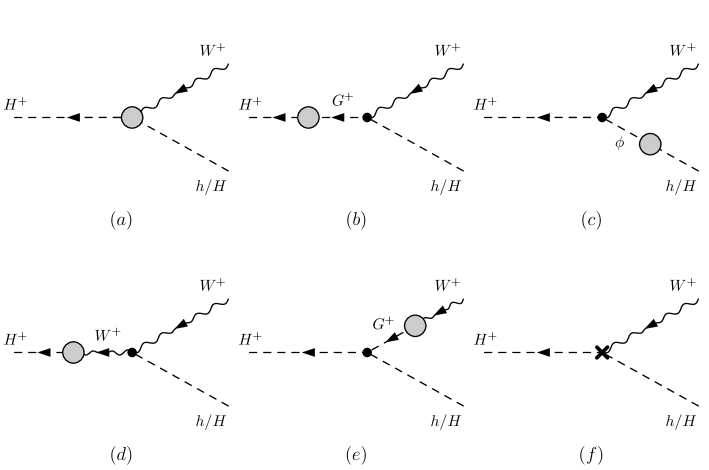
Figure 2: Generic diagrams contributing to the virtual corrections of the decays $H^{\pm}\to W^{\pm}h/H$: vertex corrections (a) and corrections to the external legs (b)-(e). Diagram (f) displays the counterterm.

and the LO decay width is given by

$$\Gamma^{\text{LO}}(H^{\pm}\to W^{\pm}\phi)=\frac{G_{F}g_{H^{\pm}W^{\pm}\phi}^{2}}{8\sqrt{2}\pi m_{H^{\pm}}^{3}}\,\lambda^{3}(m_{H^{\pm}}^{2},M_{W}^{2},m_{\phi}^{2})\;,$$ (4.8)

with

$$\lambda(x,y,z)\equiv(x^{2}+y^{2}+z^{2}-2xy-2xz-2yz)^{\frac{1}{2}}\;.$$ (4.9)

The NLO decay width can be written as

$$\Gamma^{\text{NLO}}=\Gamma^{\text{LO}}+\Gamma^{(1)}\;.$$ (4.10)

The one-loop correction $\Gamma^{(1)}$ consists of the virtual corrections, the counterterm contributions and the real corrections. The counterterms cancel the UV divergences and the real corrections the IR divergences encountered in the virtual corrections. The diagrams contributing to the latter are depicted in Fig. 2 and show the pure vertex corrections (a) and the corrections (b)-(e) to the external legs. The counterterm diagram is shown in (f). The vertex corrections comprise the 1PI diagrams given by the triangle diagrams with scalars, fermions and gauge bosons in the loops, as shown in the first two rows of Fig. 3, and the diagrams involving four-particle vertices (last four diagrams of Fig. 3).

Figure 3: Generic diagrams contributing to the vertex corrections in $H^{\pm}\to W^{\pm}h/H$.

The corrections to the external legs in Fig. 2 (b) and (c) vanish due to the OS renormalization of the scalars, while the vanishing of the mixing contribution (d) is ensured by a Slavnov-Taylor identity [59] and the one of (e) by the Ward identity for an OS $W^{\pm}$ boson. The vertex contributions with a photon in the loop lead to IR divergences that need to be canceled by the real corrections. These are computed from the diagrams displayed in Fig. 4. They consist of the proper bremsstrahlung contributions (a)-(c), where a photon is radiated from the charged initial and final state particles, and the diagram (d) involving a four-particle vertex with a photon. Note, that this last diagram leads to an IR-finite contribution.

Figure 4: Feynman diagrams contributing to the real corrections.

The NLO contributions factorize from the LO amplitude, so that the one-loop corrected decay width can be cast into the form

$$\Gamma^{\text{NLO}}(H^{\pm}\to W^{\pm}\phi)=\Gamma^{\text{LO}}\left[1+\Delta^{\text{virt}}+\Delta^{\text{ct}}+\Delta^{\text{real}}\right]\;.$$ (4.11)

The counterterm contribution $\Delta^{\text{ct}}$ is given in terms of the wave function renormalization constants, the coupling and angle counterterms. For $\phi\equiv h$ it reads

$$\Delta^{\text{ct}}=\delta Z_{WW}+\delta Z_{H^{\pm}H^{\pm}}+\delta Z_{hh}+\frac{s_{\beta-\alpha}}{c_{\beta-\alpha}}\left(\delta Z_{G^{\pm}H^{\pm}}-\delta Z_{Hh}\right)+2\frac{\delta g}{g}-2t_{\beta-\alpha}\,(\delta\beta-\delta\alpha)\;,$$ (4.12)

and for $\phi\equiv H$,

$$\Delta^{\text{ct}}=\delta Z_{WW}+\delta Z_{H^{\pm}H^{\pm}}+\delta Z_{HH}-\frac{c_{\beta-\alpha}}{s_{\beta-\alpha}}\left(\delta Z_{G^{\pm}H^{\pm}}+\delta Z_{hH}\right)+2\frac{\delta g}{g}+\frac{2(\delta\beta-\delta\alpha)}{t_{\beta-\alpha}}\;.$$ (4.13)

As the expressions for the counterterm $\Delta^{\text{ct}}$ and the virtual and real contributions $\Delta^{\text{virt}}$ and $\Delta^{\text{real}}$ in terms of scalar one-, two- and three-point functions are rather lengthy, we do not display them explicitly here.

4.2 Electroweak One-Loop Corrections to $H\to\tau\tau$ and $A\to\tau\tau$

The LO decay width for the process $H\to\tau\tau$ reads

$$\Gamma^{\text{LO}}(H\to\tau\tau)=\frac{G_{F}g^{2}_{H\tau\tau}m_{H}m_{\tau}^{2}}{4\sqrt{2}\pi}\left(1-\frac{4m_{\tau}^{2}}{m_{H}^{2}}\right)^{\frac{3}{2}}\;,$$ (4.14)

with the coupling modification factor $g_{H\tau\tau}$ in the 2HDM, which depends on the 2HDM type. We give in Table 1 the coupling factors for all neutral Higgs bosons to $\tau$ leptons in the different realizations of the 2HDM.

type	I	II	lepton-specific	flipped
$g_{h\tau\tau}$	$c_{\alpha}/s_{\beta}$	$-s_{\alpha}/c_{\beta}$	$-s_{\alpha}/c_{\beta}$	$c_{\alpha}/s_{\beta}$
$g_{H\tau\tau}$	$s_{\alpha}/s_{\beta}$	$c_{\alpha}/c_{\beta}$	$c_{\alpha}/c_{\beta}$	$s_{\alpha}/s_{\beta}$
$g_{A\tau\tau}$	$-1/t_{\beta}$	$t_{\beta}$	$t_{\beta}$	$-1/t_{\beta}$

Table 1: Neutral Higgs boson couplings to $\tau$ leptons in different realizations of the 2HDM.

For the decay $A\to\tau\tau$ the LO decay width is

$$\Gamma^{\text{LO}}(A\to\tau\tau)=\frac{G_{F}g^{2}_{A\tau\tau}m_{A}m_{\tau}^{2}}{4\sqrt{2}\pi}\sqrt{1-\frac{4m_{\tau}^{2}}{m_{A}^{2}}}\;,$$ (4.15)

with $g_{A\tau\tau}$ given in Table 1. These two processes can hence be used to define the counterterms for $\alpha$ and $\beta$.

The EW NLO corrections to $H\to\tau\tau$ consist of the virtual corrections, the counterterms and the real corrections. The generic contributions to the virtual corrections are depicted in Fig. 5.

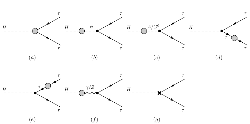
Figure 5: Generic diagrams contributing to the virtual corrections of $H\to\tau\tau$: vertex corrections (a) and corrections to the external legs (b)-(f) where $\phi\equiv h/H$. Diagram (g) displays the counterterm.

The 1PI diagrams of the vertex corrections are shown in Fig. 6 and consist of the triangle diagrams with scalars, fermions, massive gauge bosons and photons in the loop.

Figure 6: Generic diagrams contributing to the vertex corrections in $H\to\tau\tau$.

The corrections to the external legs in Fig. 5 (b), (d) and (e) vanish because of the OS renormalized $H$ and $\tau$, respectively. Diagram (c) is zero because of CP conservation. Diagram (f) finally vanishes because of a Slavnov-Taylor identity. The real corrections consist of the diagrams where a photon is radiated off either of the final state $\tau$ leptons. We explicitly checked that all NLO corrections factorize from the LO width so that the NLO decay width can be cast into the form

$$\Gamma^{\text{NLO}}(H\to\tau\tau)=\Gamma^{\text{LO}}\left[1+\Delta^{\text{virt}}+\Delta^{\text{ct}}+\Delta^{\text{real}}\right]\;.$$ (4.16)

For $\Delta^{\text{ct}}$ we have

$$\Delta^{\text{ct}} = \delta Z_{HH}+\frac{g_{h\tau\tau}}{g_{H\tau\tau}}\delta Z_{hH}+\delta Z_{\tau\tau}^{L}+\delta Z_{\tau\tau}^{R}+2\frac{\delta g}{g}+2\frac{\delta m_{\tau}}{m_{\tau}}-\frac{\delta M_{W}^{2}}{M_{W}^{2}}$$ (4.17)

$$+\frac{2g_{h\tau\tau}}{g_{H\tau\tau}}\,\delta\alpha+2g_{A\tau\tau}\,\delta\beta\;.$$

Note, that the pure QED contributions in $\Delta^{{\text{virt}}}$ and $\Delta^{\text{ct}}$ can be separated from the weak contributions in a gauge-invariant way and form a UV-finite subset by themselves. This is important as it allows to define the angular counterterm via this process through the purely weak NLO contributions, see also the discussion in section 3.1.4. Requiring the following renormalization condition for the process-dependent definition of $\delta\alpha$,

$$\Gamma^{\text{LO}}(H\to\tau\tau)\stackrel{{\scriptstyle!}}{{=}}\Gamma_{\text{weak}}^{\text{NLO}}(H\to\tau\tau)\;,$$ (4.18)

and imposing this condition only on the weak part of the decay width we arrive at the process-dependent counterterm definition

$$\delta\alpha^{H\to\tau\tau} = -\frac{g_{H\tau\tau}}{2g_{h\tau\tau}}\left[\delta Z_{HH}+\frac{g_{h\tau\tau}}{g_{H\tau\tau}}\delta Z_{hH}+\delta Z_{\tau\tau}^{L,\text{weak}}+\delta Z_{\tau\tau}^{R,\text{weak}}+2\frac{\delta g}{g}+2\frac{\delta m_{\tau}^{\text{weak}}}{m_{\tau}}-\frac{\delta M_{W}^{2}}{M_{W}^{2}}\right.$$ (4.19)

$$\left.+\,2g_{A\tau\tau}\,\delta\beta+\Delta^{\text{virt,weak}}_{H\to\tau\tau}\right]\;.$$

The superscript ’weak’ indicates that in the respective counterterms and in the virtual correction only the purely weak contributions are taken into account. For example for $\Delta^{\text{virt,weak}}_{H\to\tau\tau}$ this means that corrections stemming from diagrams in Fig. 6 that involve photons are dropped.

The counterterm $\delta\tan\beta$ or $\delta\beta$, respectively, which is necessary in (4.19), can be defined in a process-dependent scheme via the NLO decay $A\to\tau\tau$ as outlined in the following. Again the NLO contributions consist of virtual, counterterm and real diagrams.

Figure 7: Generic diagrams contributing to the virtual corrections of $A\to\tau\tau$: vertex corrections (a) and corrections to the external legs (b)-(f), where $\phi\equiv h/H$. Diagram (g) displays the counterterm.

Figure 8: Generic diagrams contributing to the vertex corrections in $A\to\tau\tau$.

The generic ones for the former two are shown in Fig. 7 and the 1PI diagrams of the vertex corrections are summarized in Fig. 8. The loops contain scalars, fermions, massive gauge bosons and photons. The loops with photons induce IR divergences that are canceled by the real corrections. The corrections to the external legs in Fig. 7 (b), (d) and (e) vanish due to OS renormalization conditions, those in (c) because of CP invariance and those in (f) because of a Slavnov-Taylor identity. Also in this process the pure QED corrections can be separated from the remainder in a gauge-invariant way and form a UV-finite subset so that the NLO decay width can be used for the process-dependent definition of the counterterm $\delta\beta$ through the requirement

$$\Gamma^{\text{LO}}(A\to\tau\tau)\stackrel{{\scriptstyle!}}{{=}}\Gamma^{\text{NLO}}_{\text{weak}}(A\to\tau\tau)\;.$$ (4.20)

With the factorization

$$\Gamma^{\text{NLO}}(A\to\tau\tau)=\Gamma^{\text{LO}}\left[1+\Delta^{\text{virt}}+\Delta^{\text{ct}}+\Delta^{\text{real}}\right]$$ (4.21)

and the counterterm

$$\Delta^{\text{ct}} = \delta Z_{AA}-\frac{1}{g_{A\tau\tau}}\delta Z_{G^{0}A}+\delta Z_{\tau\tau}^{L}+\delta Z_{\tau\tau}^{R}+2\frac{\delta g}{g}+2\frac{\delta m_{\tau}}{m_{\tau}}-\frac{\delta M_{W}^{2}}{M_{W}^{2}}$$ (4.22)

$$+\frac{2(1+g^{2}_{A\tau\tau})}{g_{A\tau\tau}}\,\delta\beta$$

we arrive by imposing the condition (4.20) at

$$\delta\beta^{A\to\tau\tau}= \frac{-g_{A\tau\tau}}{2(1+g_{A\tau\tau}^{2})}\left[\delta Z_{AA}-\frac{1}{g_{A\tau\tau}}\delta Z_{G^{0}A}+\delta Z_{\tau\tau}^{L,\text{weak}}+\delta Z_{\tau\tau}^{R,\text{weak}}+2\frac{\delta g}{g}+2\frac{\delta m_{\tau}^{\text{weak}}}{m_{\tau}}\right.$$ (4.23)

$$\left.-\frac{\delta M_{W}^{2}}{M_{W}^{2}}+\Delta^{\text{virt,weak}}_{A\to\tau\tau}\right]\;.$$

Again the superscript ’weak’ denotes the purely weak contributions to the respective counterterms and to the virtual corrections. Thus, $\Delta^{\text{virt,weak}}_{A\to\tau\tau}$ is given by the purely weak virtual corrections to $A\to\tau\tau$ at NLO which are computed from the diagrams in Fig. 8 discarding those with photons in the loop.

4.3 The gauge (in)dependence of the angular counterterms

The question of gauge dependence in the standard scheme: In order to investigate the question whether the angular counterterms can be defined in a gauge-independent way, we have calculated the one-loop corrected decay width for the charged Higgs decays in the general $R_{\xi}$ gauge. When we apply the standard scheme, the computation of the NLO amplitude ${\cal M}_{H^{\pm}\to W^{\pm}h}$ including all counterterms but the one for the angles - i.e. $\delta c_{\beta-\alpha}$ is set to zero - yields an amplitude that depends on the gauge parameters as follows,

$$\left.{\cal M}_{H^{\pm}\to W^{\pm}h}\right|^{\text{standard}}_{\text{NLO, }\xi,\,\delta c_{\beta-\alpha}=0} = -\frac{g\Lambda_{5}c_{\beta-\alpha}s^{2}_{\beta-\alpha}\,p_{1}\cdot\epsilon^{*}(p_{3})}{32\pi^{2}(m_{H}^{2}-m_{h}^{2})}\left[2M_{W}^{2}(1-\xi_{W})\alpha_{W}\right.$$ (4.24)

$$\left.+M_{Z}^{2}(1-\xi_{Z})\alpha_{Z}\right]\;,$$

where we have introduced the abbreviation ($V\equiv W,Z$)

$$\begin{split}\alpha_{V}&=\frac{1}{(1-\xi_{V})m_{V}^{2}}\left[A_{0}(m_{V}^{2})-A_{0}(\xi_{V}m_{V}^{2})\right]\end{split}$$ (4.25)

in terms of the scalar one-point function $A_{0}$ [27, 28]. With $p_{1}$ we denote the incoming four-momentum of $H^{\pm}$ and with $\epsilon^{*}(p_{3})$ the polarization vector of the outgoing $W^{\pm}$ boson with four-momentum $p_{3}$ and

$$\Lambda_{5}\equiv\frac{2m_{12}^{2}}{v^{2}s_{\beta}c_{\beta}}\;.$$ (4.26)

Note that $\alpha_{V}$ is UV-divergent. This result shows explicitly what we have already stated before: In the standard renormalization scheme, the NLO decay amplitude without the angular counterterms has a residual UV-divergent gauge dependence. This can only be canceled by the angular counterterms. Therefore, the counterterms cannot be defined in a gauge-independent way. This gauge dependence is independent of the renormalization scheme chosen for the angular counterterms. It is purely due to the treatment of the tadpoles. Let us investigate what happens if we apply the KOSY scheme, which yields the renormalization conditions Eq. (3.110) and Eq. (3.111) or Eq. (3.112), respectively. Introducing the UV-finite integral

$$\beta_{Vj}(p^{2})=\frac{1}{(1-\xi_{V})m_{V}^{2}}\left[B_{0}(p^{2};m_{V}^{2},m_{j}^{2})-B_{0}(p^{2};\xi_{V}m_{V}^{2},m_{j}^{2})\right]$$ (4.27)

in terms of the scalar two-point function $B_{0}$, we find the following gauge-dependent results for the angular counterterms,

$$\delta\alpha = \left.\delta\alpha\right|_{\xi=1}$$

$$-\frac{\Lambda_{5}c_{\beta-\alpha}s_{\beta-\alpha}}{32\pi^{2}(m_{H}^{2}-m_{h}^{2})}\left[2M_{W}^{2}(1-\xi_{W})\alpha_{W}+M_{Z}^{2}(1-\xi_{Z})\alpha_{Z}\right]$$

$$+(1-\xi_{Z})\frac{g^{2}c_{\beta-\alpha}s_{\beta-\alpha}}{256\pi^{2}c_{W}^{2}}\bigg{\{}2m_{A}^{2}\Big{[}\beta_{ZA}(m_{H}^{2})-\beta_{ZA}(m_{h}^{2})\Big{]}$$

$$\hskip 5.69046pt+m_{H}^{2}\Big{[}\beta_{Z\xi Z}(m_{H}^{2})-2\beta_{ZA}(m_{H}^{2})\Big{]}-m_{h}^{2}\Big{[}\beta_{Z\xi Z}(m_{h}^{2})-2\beta_{ZA}(m_{h}^{2})\Big{]}\bigg{\}}$$

$$+(1-\xi_{W})\frac{g^{2}c_{\beta-\alpha}s_{\beta-\alpha}}{128\pi^{2}}\bigg{\{}2m_{H^{\pm}}^{2}\Big{[}\beta_{WH^{\pm}}(m_{H}^{2})-\beta_{WH^{\pm}}(m_{h}^{2})\Big{]}$$

$$\hskip 5.69046pt+m_{H}^{2}\Big{[}\beta_{W\xi W}(m_{H}^{2})-2\beta_{WH^{\pm}}(m_{H}^{2})\Big{]}-m_{h}^{2}\Big{[}\beta_{W\xi W}(m_{h}^{2})-2\beta_{WH^{\pm}}(m_{h}^{2})\Big{]}\bigg{\}},$$ (4.28)

and

$$\begin{split}\delta\beta^{(1)}=&\left.\delta\beta^{(1)}\right|_{\xi=1}\\ &+\left(1-\xi_{W}\right)\frac{g^{2}c_{\beta-\alpha}s_{\beta-\alpha}}{128\pi^{2}}\bigg{\{}m_{h}^{2}\Big{[}\beta_{Wh}(m_{H^{\pm}}^{2})-\beta_{Wh}(0)\Big{]}\\ &+m_{H^{+}}^{2}\Big{[}\beta_{WH}(m_{H^{\pm}}^{2})-\beta_{Wh}(m_{H^{\pm}}^{2})\Big{]}+m_{H}^{2}\Big{[}\beta_{WH}(0)-\beta_{WH}(m_{H^{\pm}}^{2})\Big{]}\bigg{\}}~{}.\end{split}$$ (4.29)

Here the symbol $\big{|}_{\xi=1}$ represents the counterterm result obtained for $\xi=\xi_{W}=\xi_{Z}=1$. The result for $\delta\beta^{(2)}$ looks similar with the appropriate mass replacements and $\xi_{W}\to\xi_{Z}$. The second line in Eq. (4.28) has the appropriate structure to cancel the remaining UV-divergent gauge dependence in the amplitude (4.24). However, the additional finite terms in (4.28) and (4.29) proportional to the $\beta$-integrals defined above, reintroduce a gauge dependence into the amplitude. In [24] it was argued that the gauge dependence of $\delta\beta$ can be moved into the unphysical counterterm $\delta C_{f}$, see Eq. (3.99). Yet, lacking a method to define uniquely the gauge-dependent parts in the standard scheme, where the PT cannot be applied, it remains unclear, how this could be accomplished. The situation is even worse for $\delta\alpha$, where we necessarily have to retain the gauge-dependent part proportional to the UV-divergent $A_{0}$ functions, but must move the rest into $\delta C_{f}$. To summarize, this result shows that not only is it impossible to arrive at a gauge-independent definition of $\delta\alpha$ in the standard scheme, but it also explicitly demonstrates that the KOSY scheme leads to an unphysical gauge dependence of the decay amplitude, which one cannot be disposed of in a straightforward way. This is not only true for the charged Higgs bosons decays we are discussing. In fact, the investigation of the origin of this gauge dependence shows, that the standard tadpole scheme inevitably leads to gauge-dependent decay widths in case the KOSY scheme is applied for the mixing angles.

If we define the angular counterterms via a physical process, however, namely through the decay widths $H\to\tau\tau$ and $A\to\tau\tau$, compute the contribution of the counterterm $\delta c_{\beta-\alpha}$, and extract the $\xi$-dependent parts we obtain the following,

$$\left.{\cal M}_{H^{\pm}\to W^{\pm}h}\right|^{\text{standard}}_{\text{ct, }\xi,\,\delta c_{\beta-\alpha}\text{ only}} = \frac{g\Lambda_{5}c_{\beta-\alpha}s^{2}_{\beta-\alpha}\,p_{1}\cdot\epsilon^{*}(p_{3})}{32\pi^{2}(m_{H}^{2}-m_{h}^{2})}\left[2M_{W}^{2}(1-\xi_{W})\alpha_{W}\right.$$ (4.30)

$$\left.+M_{Z}^{2}(1-\xi_{Z})\alpha_{Z}\right]\;.$$

It is exactly the same as Eq. (4.24) but with opposite sign, so that altogether the EW one-loop corrected decay width is gauge independent and UV-finite as required. The standard treatment of the tadpoles combined with a process-dependent definition hence leads to a gauge-independent physical result, as it should be. The counterterms, however, necessarily contain a gauge dependence.

Gauge-independent angular counterterms: For the angular counterterms to be gauge-independent the loop-corrected amplitude including all counterterms but the angular ones must be independent of $\xi$. This can be achieved by treating the tadpoles according to Ref. [29], cf. the discussion in section 3.1.3. It means that in the counterterms Eq. (4.12) and Eq. (4.13), respectively, the self-energies $\Sigma$ and the tadpole counterterms $\delta T$, contained in the wave function constants, the scalar mass counterterms and the angular counterterms, have to be replaced by $\Sigma^{\text{tad}}$ and $\delta T=0$. Note, that the change to this tadpole scheme in principle implies new vertices arising from constant tadpole contributions to the respective original vertices, cf. App. A. In the 2HDM, however, there is no quartic vertex between two scalars, a charged Higgs and a charged gauge boson, $h/H-h/H-H^{\pm}-W^{\mp}$, where one of the external $h/H$ legs would carry the additional tadpole contribution. Therefore, the process $H^{\pm}\to W^{\pm}h/H$ does not receive additional tadpole diagrams. The counterterms $\delta\alpha$, $\delta\beta$, $\delta Z_{hH}$, $\delta Z_{Hh}$ $\delta Z_{G^{0}A}$ and $\delta Z_{G^{\pm}H^{\pm}}$ change however. With these modifications the gauge-dependent part of the amplitude with the angular counterterms set to zero, becomes

$$\left.{\cal M}_{H^{\pm}\to W^{\pm}h}\right|_{\text{NLO, }\xi,\,\delta c_{\beta-\alpha}=0}^{\text{tad}}=0\;.$$ (4.31)

The amplitude without the mixing angle counterterm is itself gauge-independent, so that it is possible to provide a gauge-independent renormalization of the angular counterterms.

a) Gauge-independent tadpole-pinched scheme: The pinch technique allows to extract from the Green functions the truly gauge-independent part. Combined with the tadpole scheme this leads to manifestly gauge-independent angular counterterms. Choosing the OS scale, they are given by Eqs. (3.136)-(3.141). In the $p_{\star}$ scheme the formulae simplify to (3.144)-(3.146). In the numerical analysis we will apply both choices.

b) Gauge-independent process-dependent definition of the angular counterterms: Another possibility to arrive at a truly gauge-independent definition of the angular counterterms is the definition via the physical processes $H/A\to\tau\tau$, provided of course that the framework of the tadpole scheme is applied.

In the processes $H/A\to\tau\tau$ no new diagrams are introduced when switching to the tadpole scheme, while the counterterms do change. In the tadpole scheme the process-dependent definition of $\delta\alpha$ and $\delta\beta$ through the requirement Eq. (4.18) and Eq. (4.20), respectively, then indeed leads to gauge independence of both counterterms and hence also of $\delta c_{\beta-\alpha}$, i.e.

$$(\delta c_{\beta-\alpha})^{\text{tad, proc-dep}}_{\xi}=0\;.$$ (4.32)

We have seen in Eq. (4.30) that the treatment of the tadpoles in the standard scheme cannot lead to gauge-independent angular counterterms, although they are defined through a physical process. In detail, this gauge parameter dependence stems from $\delta\alpha$, whereas $\delta\beta$ is gauge-independent in the process-dependent definition also without applying the tadpole scheme. Thus we have

$$\delta\beta^{\text{proc-dep}}_{\xi} = \delta\beta^{\text{tad, proc-dep}}_{\xi}=0$$ (4.33)

$$\delta\alpha^{\text{tad, proc-dep}}_{\xi} = 0$$ (4.34)

$$\delta\alpha^{\text{proc-dep}}_{\xi} = -\frac{\Lambda_{5}c_{\beta-\alpha}s_{\beta-\alpha}}{32\pi^{2}(m_{H}^{2}-m_{h}^{2})}\left[2M_{W}^{2}(1-\xi_{W})\alpha_{W}+M_{Z}^{2}(1-\xi_{Z})\alpha_{Z}\right]\,.$$ (4.35)

This result shows two important things: First, the process-dependent definition of the angular counterterms leads to gauge-independent counterterms only if the tadpole scheme is applied. Second, Eqs. (4.33)-(4.35) demonstrate, that in a process-dependent definition of the counterterms the difference between the application of the tadpole and the standard scheme is a gauge-dependent expression that solely depends on $A_{0}$ functions, which are UV-divergent. As the 2HDM is renormalizable this implies that also in the amplitude the difference in the application of the two schemes must be UV-divergent and must have the same structure, since the divergences have to cancel. In conclusion, this means: The definition of the angular counterterms via any physical process leads for any NLO decay process to a gauge-independent result, independently of the treatment of the tadpoles.

In the following numerical analysis in section 5 we will apply all three types of renormalization schemes, the standard, the tadpole-pinched and the process-dependent scheme, and compare them to each other. We will do this for the sample processes $H^{\pm}\to W^{\pm}h/H$ and $H\to ZZ$. In order to describe also for this latter process the implications of the tadpole scheme, required for a gauge-independent definition of the angular counterterms, we briefly repeat the ingredients of the EW one-loop corrections to $H\to ZZ$.

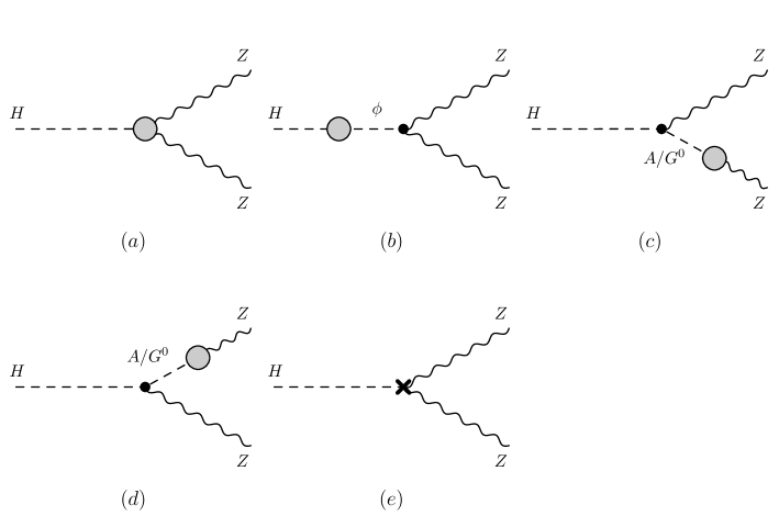
Figure 9: Generic diagrams contributing to the virtual corrections of the decay $H\to ZZ$: vertex corrections (a) and corrections to the external legs (b)-(d) where $\phi\equiv h,H$. Diagram (e) displays the counterterm.

4.4 Electroweak One-Loop Corrections to $H\to ZZ$

The LO decay width for the process

$$H\to ZZ$$ (4.36)

is given by

$$\Gamma^{\text{LO}}(H\to ZZ)=\frac{G_{F}g_{HZZ}^{2}}{32\sqrt{2}\pi m_{H}}(m_{H}^{4}-4m_{H}^{2}m_{Z}^{2}+12m_{Z}^{4})\sqrt{1-\frac{4M_{Z}^{2}}{m_{H}^{2}}}$$ (4.37)

and depends on the mixing angles through the coupling factor

$$g_{HZZ}=c_{\beta-\alpha}\;.$$ (4.38)

The NLO decay width consists of virtual corrections and the counterterm contributions to cancel the UV divergences. There are neither IR divergences nor real corrections. The generic diagrams for the virtual corrections and the counterterm are depicted in Fig. 9. The 1PI diagrams contributing to the vertex corrections are given by the triangle diagrams with scalars, fermions, massive gauge bosons and ghost particles in the loops, as shown in the first three rows of Fig. 10, and by the diagrams involving four-particle vertices (last four diagrams of Fig. 10).

Figure 10: Generic diagrams contributing to the vertex corrections in $H\to ZZ$. The ghost particles are denoted by $U$.

The corrections to the external leg in Fig. 9 (b) vanish due to the OS renormalization of the $H$. The mixing contributions (c) and (d) vanish because of the Ward identity for the OS $Z$ boson. The counterterm amplitude is given by

$${\cal M}_{H\to ZZ}^{\text{ct}} = \frac{ec_{\beta-\alpha}M_{W}}{c_{W}^{2}s_{W}}\epsilon^{*}(p_{3})\cdot\epsilon^{*}(p_{4})$$ (4.39)

$$\times \left[\frac{\delta g}{g}+\frac{\delta c_{\beta-\alpha}}{c_{\beta-\alpha}}+\frac{\delta M_{Z}^{2}}{M_{Z}^{2}}-\frac{\delta M_{W}^{2}}{2M_{W}^{2}}+\frac{s_{\beta-\alpha}}{c_{\beta-\alpha}}\,\frac{\delta Z_{hH}}{2}+\frac{\delta Z_{HH}}{2}+\delta Z_{ZZ}\right]\,,$$

where the $\epsilon^{\mu*}$ denote the polarization vectors of the outgoing $Z$ bosons with four-momentum $p_{3}$ and $p_{4}$, respectively. If the tadpole scheme is applied, the $HZZ$ vertex is modified by additional tadpole contributions, which lead to further diagrams, that have to be taken into account in the computation of the decay width. They are shown in Fig. 11. As the formula for the vertex corrections and counterterms in terms of the scalar one-, two- and three-point functions are quite lengthy, we do not display them explicitly here.

Figure 11: Additional vertex diagrams in the tadpole scheme contributing to the decay $H\to ZZ$.

5 Numerical Analysis

For the computation of the NLO EW corrections to the Higgs decay widths described in the previous section we have performed two independent calculations. Both of them employed the Mathematica package FeynArts 3.9 [62, 63] to generate the amplitudes at LO and NLO in the general $R_{\xi}$ gauge. To this end, the model file for a CP-conserving 2HDM was used, which is already implemented in the package. Additionally, all tadpole and self-energy amplitudes, needed for the definition of the counterterms and wave function renormalization constants, have been generated in the general $R_{\xi}$ gauge. The contraction of the Dirac matrices and formulation of the results in terms of Passarino-Veltman functions has been done with FeynCalc 8.2.0 [64] in one calculation and with FormCalc [65] in the other. The dimensionally regularized [66, 67] integrals have been evaluated numerically with the help of the C++ library LoopTools 2.12 [65].

For one of the two calculations the Python progam 2HDMCalc was developed that links FeynArts, generates the needed counterterms dynamically from the 2HDM Lagrangian by calling a Mathematica script and combines the LO, NLO and counterterms calculated by FeynCalc into the full partial decay widths. These are then evaluated numerically by linking LoopTools. Finally, the LO and NLO partial decay widths are written out for all renormalization schemes of the mixing angles introduced above. The outcome of this program was compared to the results of the second independent computation. All results agree within numerical errors.

In the following we specify the input parameters that we used for the numerical evaluation. As explained in section 3 we use the fine structure constant $\alpha$ at the $Z$ boson mass scale, given by [68]

$$\alpha(M_{Z}^{2})=\frac{1}{128.962}\;.$$ (5.1)

The massive gauge boson masses are set to [68, 69]

$$M_{W}=80.385\mbox{ GeV}\qquad\mbox{and}\qquad M_{Z}=91.1876\mbox{ GeV}\;.$$ (5.2)

For the lepton masses we choose [68, 69]

$$m_{e}=0.510998928\mbox{ MeV}\;,\quad m_{\mu}=105.6583715\mbox{ MeV}\;,\quad m_{\tau}=1.77682\mbox{ GeV}\;.$$ (5.3)

These and the light quark masses, which we set [70]

$$m_{u}=100\mbox{ MeV}\;,\quad m_{d}=100\mbox{ MeV}\;,\quad m_{s}=100\mbox{ MeV}\;,$$ (5.4)

have only a small influence on our results. In order to be consistent with the ATLAS and CMS analyses, we follow the recommendation of the LHC Higgs Cross Section Working Group (HXSWG) [69, 71] and use the following OS value for the top quark mass

$$m_{t}=172.5\mbox{ GeV}\;.$$ (5.5)

The charm and bottom quark OS masses are set to

$$m_{c}=1.51\mbox{ GeV}\qquad\mbox{and}\qquad m_{b}=4.92\mbox{ GeV}\;,$$ (5.6)

as recommended by [69]. Omitting CP violation we consider the CKM matrix to be real, with the CKM matrix elements given by [68]

$$V_{\text{CKM}}=\left(\begin{array}[]{ccc}V_{ud}&V_{us}&V_{ub}\\ V_{cd}&V_{cs}&V_{cb}\\ V_{td}&V_{ts}&V_{tb}\end{array}\right)=\left(\begin{array}[]{ccc}0.97427&0.22536&0.00355\\ -0.22522&0.97343&0.0414\\ 0.00886&-0.0405&0.99914\end{array}\right)\;.$$ (5.13)

The SM-like Higgs mass value, denoted by $m_{H_{\text{SM}}}$, has been set to [72]

$$m_{H^{\text{SM}}}=125.09\mbox{ GeV}\;.$$ (5.14)

Note, that in the 2HDM, depending on the chosen parameter set, it is possible that either the lighter or the heavier of the two CP-even neutral Higgs bosons can be the SM-like Higgs boson.

The IR divergences in the computation of the NLO corrections to the process $H^{\pm}\to W^{\pm}H/h$ require the inclusion of the real corrections to regularize the decay width. This introduces a dependence on the detector sensitivity $\Delta E$ for the resolution of the soft photons from the real corrections. We showed that this dependence is small [73]. For our analysis we fixed the value to

$$\Delta E=10\mbox{ GeV}\;.$$ (5.15)

In the subsequently presented plots we only used 2HDM parameter sets that are not yet excluded by experiment and that fulfill certain theoretical constraints. These data sets have been generated with the tool ScannerS [74]. The applied theoretical constraints require that the chosen CP-conserving vacuum is the global minimum [75], that the 2HDM potential is bounded from below [76] and that tree-level unitarity holds [77, 78]. For consistency with experimental data the following conditions have been imposed. The electroweak precision constraints [79, 80, 81, 82, 83, 84, 85] have to be satisfied, i.e. the $S,T,U$ variables [79] predicted by the model are within the 95% ellipsoid centered on the best fit point to the EW data. Indirect experimental constraints are due to loop processes involving charged Higgs bosons, that depend on $\tan\beta$ via the charged Higgs coupling to the fermions. They are mainly due to $B$ physics observables [86, 87, 88] and the measurement of $R_{b}$ [89, 90, 91, 92]. We have included the most recent bound of $m_{H^{\pm}}\raisebox{-3.69899pt}{~{}\shortstack{$>$ \\ [-0.07cm] $\sim$}}~{}480$ GeV for the type II and flipped 2HDM [93]. The results from LEP [94] and the recent ones from the LHC [95, 96] constrain the charged Higgs mass to be above ${\cal O}(100\mbox{ GeV})$ depending on the model type. In order to check the compatibility with the LHC Higgs data ScannerS is interfaced with SusHi [98] which computes the Higgs production cross sections through gluon fusion and $b$-quark fusion at NNLO QCD. All other production cross sections are taken at NLO QCD [70]. The 2HDM decays were obtained from HDECAY [99, 100]. Note that in the computation of these processes all EW corrections were consistently neglected, as they are not available for the 2HDM. The exclusion limits were checked by using HiggsBounds [101, 102, 103] and the compatibility with the observed signal for the 125 GeV Higgs boson was tested with HiggsSignals [104]. For further details we refer to [105].

In our numerical analysis we investigate the applicability of the various proposed renormalization schemes. The goal is to find a renormalization scheme for the 2HDM, that is process independent, gauge independent and numerically stable. All results that we show are for the 2HDM type II.

5.1 Gauge dependence of the KOSY scheme

We start by analyzing the gauge dependence of the partial decay width, introduced through the renormalization of the mixing angles $\alpha$ and $\beta$ in the KOSY scheme. As an example we choose the charged Higgs boson decay into the $W$ boson and the light CP-even scalar $h$ corresponding to $H^{\text{SM}}$, $H^{\pm}\to W^{\pm}h$. For the renormalization of $\beta$ we use the charged sector and call the renormalization scheme accordingly KOSY^c. The corresponding angular counterterm $\delta\beta^{(1)}$ is defined in Eqs. (3.111), while $\delta\alpha$ is given by Eq. (3.110). The size of the gauge dependence will be quantified by

$$\Delta\Gamma_{\xi}\equiv\frac{\Gamma^{\text{NLO}}_{\xi}-\Gamma^{\text{NLO}}_{\xi=1}}{\Gamma^{\text{NLO}}_{\xi=1}}\;.$$ (5.16)

It parametrizes the deviation of the NLO partial decay width for an arbitrarily chosen gauge parameter $\xi$ in the $R_{\xi}$ gauge from the reference decay width chosen to be the NLO width in the Feynman gauge, normalized to the reference value. For simplicity we only vary the gauge parameter $\xi_{W}$ and set $\xi_{Z}=1$. The 2HDM scenario Scen1 that we investigate is defined by the input parameters

$$\begin{array}[]{llll}\mbox{\it\text@underline{Scen1:}}&\;m_{H^{\pm}}=780\mbox{ GeV}\,,&\;m_{H}=742.84\mbox{ GeV}\,,&\;m_{A}=700.13\mbox{ GeV}\,,\\ &\;\tan\beta=1.46\,,&\;\alpha=-0.57\,,&\;m_{12}^{2}=2.076\cdot 10^{5}\mbox{ GeV}^{2}\,.\end{array}$$ (5.19)

Figure 12 shows the $\xi_{W}$ dependence of our process, $\Delta_{\xi_{W}}^{H^{\pm}W^{\pm}h}$, as a function of $\xi_{W}$. The kinks in the figure are due to threshold effects in the $B_{0}$ functions entering the counterterms. In detail, the kinks are given by the following parameter configurations and counterterms

Kink	$\xi_{W}$	Kinematic point	Origin
1	0.2137	$m_{H^{\pm}}\approx m_{H}+\sqrt{\xi_{W}}m_{W}$	$\delta\beta^{(1)}$
2	0.60539	$m_{h}\approx\sqrt{\xi_{W}}m_{W}+\sqrt{\xi_{W}}m_{W}$	$\delta\alpha$
3	21.3491	$m_{H}\approx\sqrt{\xi_{W}}m_{W}+\sqrt{\xi_{W}}m_{W}$	$\delta\alpha$
4	66.3763	$m_{H^{\pm}}\approx m_{h}+\sqrt{\xi_{W}}m_{W}$	$\delta\beta^{(1)}$

With a relative variation of the NLO width of up to 20% due to the change of the gauge parameter, the figure clearly demonstrates the gauge dependence of the NLO decay width in the KOSY scheme. The explicit calculation shows that for large values of $\xi_{W}$ the partial decay width drops as $-(m_{H}^{2}-m_{h}^{2})\ln(\xi_{W})$. This explicit gauge dependence makes a practical use of the KOSY scheme impossible as it leads to non-physical gauge dependences in the decay widths.

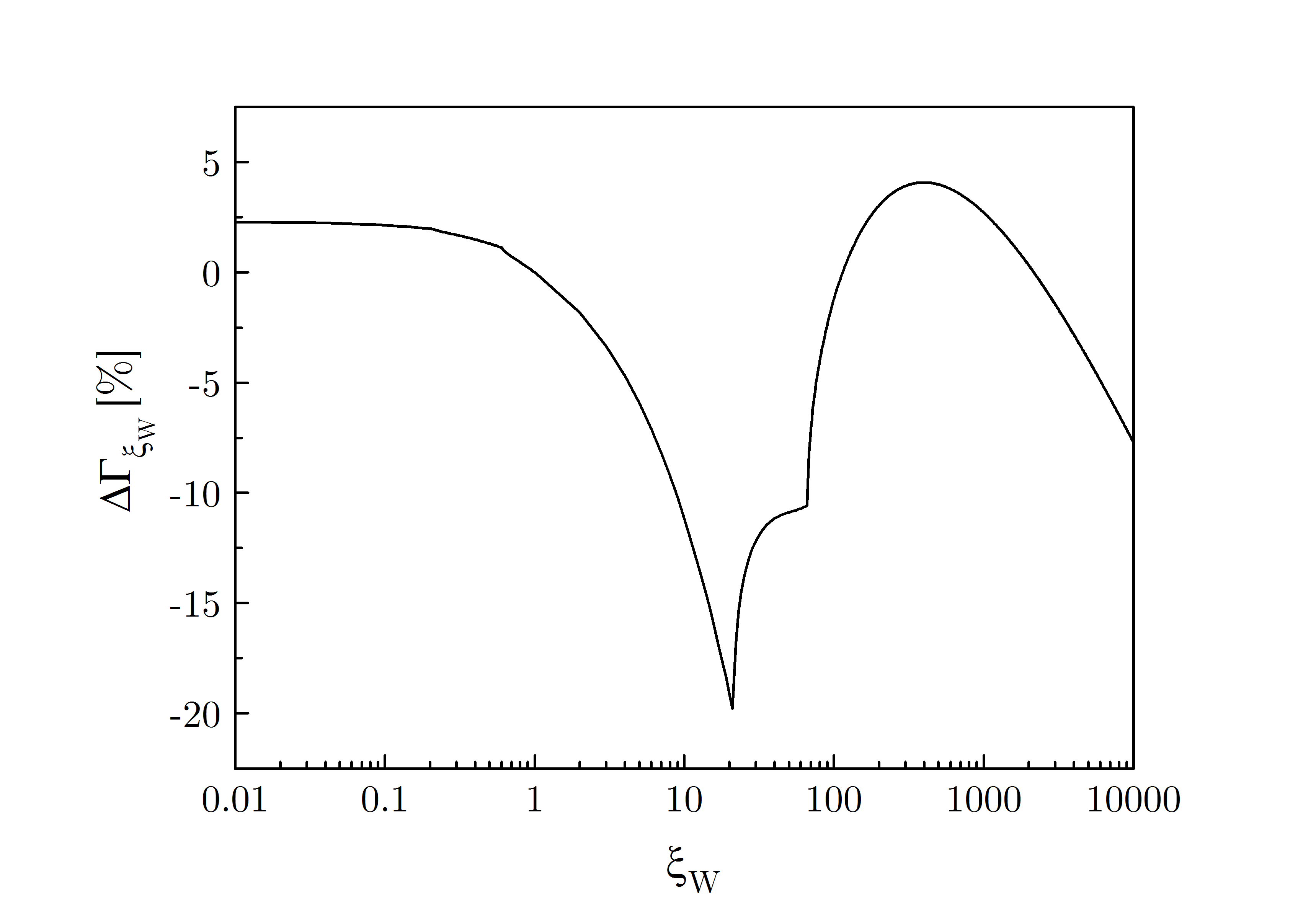
Figure 12: Gauge dependence of the decay $H^{\pm}\to W^{\pm}h$ within the KOSY^c scheme. The 2HDM parameters are given by Scen1 defined in Eq. (5.19).

5.2 The processes $\Gamma(H^{\pm}\to W^{\pm}h/H)$ at NLO

We move on to the investigation of the size of the NLO corrections to the processes $H^{\pm}\to W^{\pm}h/H$ and their dependence on the renormalization scheme. In our scenarios $h$ corresponds to the SM-like Higgs bosons. We define the quantity

$$\Delta\Gamma\equiv\frac{\Gamma^{\text{NLO}}-\Gamma^{\text{LO}}}{\Gamma^{\text{LO}}}\;,$$ (5.20)

which measures the relative size of the NLO corrections compared to the LO decay width. For the discussion of the $H^{\pm}\to W^{\pm}h$ decay we chose among the generated valid scenarios again the one given by Scen1, but this time vary the charged Higgs boson mass. For distinction, we call it Scen2 and it is given by

$$\begin{array}[]{llll}\mbox{\it\text@underline{Scen2:}}&\;m_{H^{\pm}}=(654...804)\mbox{ GeV}\,,&\;m_{H}=742.84\mbox{ GeV}\,,&\;m_{A}=700.13\mbox{ GeV}\,,\\ &\;\tan\beta=1.46\,,&\;\alpha=-0.57\,,&\;m_{12}^{2}=2.076\cdot 10^{5}\mbox{ GeV}^{2}\,.\end{array}$$ (5.23)

For $H^{\pm}\to W^{\pm}H$ we chose Scen3 where the mass $m_{A}$ is varied,

$$\begin{array}[]{llll}\mbox{\it\text@underline{Scen3:}}&\;m_{H^{\pm}}=745.54\mbox{ GeV}\,,&\;m_{H}=594.55\mbox{ GeV}\,,&\;m_{A}=(704...735)\mbox{ GeV}\,,\\ &\;\tan\beta=1.944\,,&\;\alpha=-0.458\,,&\;m_{12}^{2}=1.941\cdot 10^{5}\mbox{ GeV}^{2}\,.\end{array}$$ (5.26)

In Fig. 13 we show the relative NLO corrections for $H^{\pm}\to W^{\pm}h$, $\Delta\Gamma^{H^{\pm}W^{\pm}h}$, as a function of the charged Higgs boson mass for various renormalization schemes. We denote them as

$$\begin{array}[]{lll}\mbox{proc}&:&\quad\mbox{process-dependent}\\ p_{\star}^{c,o}&:&\quad p_{\star}\mbox{ tadpole-pinched},\;\delta\beta^{(1)}\mbox{ ('$c$') or }\delta\beta^{(2)}\mbox{ ('$o$')}\\ \mbox{pOS}^{c,o}&:&\quad\mbox{on-shell tadpole-pinched},\;\delta\beta^{(1)}\mbox{ or }\delta\beta^{(2)}\\ \mbox{KOSY}^{c,o}&:&\quad\mbox{gauge-dependent scheme},\;\delta\beta^{(1)}\mbox{ or }\delta\beta^{(2)}\;.\end{array}$$ (5.31)

The process-dependent renormalization refers to the renormalization of $\alpha$ via the process $H\to\tau\tau$ and of $\beta$ via $A\to\tau\tau$. The process-dependent renormalization can be performed by applying either the standard or the alternative tadpole scheme. The investigation of the decay widths shows, however, that all decays discussed in this analysis, i.e. $H^{\pm}\to W^{\pm}h/H$ and $H\to ZZ$, are invariant with respect to a change of the tadpole scheme. In the process-independent schemes we can choose to renormalize $\beta$ either through the charged sector, with the counterterm given by $\delta\beta^{(1)}$, or through the CP-odd sector, with the counterterm given by $\delta\beta^{(2)}$. For the shown $m_{H^{\pm}}$ range the LO decay width varies from $\Gamma^{\text{LO}}=0.0750$ GeV at $m_{H^{\pm}}=654$ GeV to $\Gamma^{\text{LO}}=0.1474$ GeV at $m_{H^{\pm}}=804$ GeV.

In Fig. 13 (left) we show results for the process-dependent renormalization and for some representatives of the process-independent schemes, the pOS^o, the $p_{\star}^{c}$ and for comparison also the KOSY^c scheme. As can be inferred from the left plot, the process-dependent renormalization leads to much larger NLO corrections than the other schemes. The NLO corrections can increase the LO width by more than a factor of three. For the process-independent renormalization schemes on the other hand, the NLO corrections are much milder and vary between about $-11$ to $20$% depending on the renormalization scheme and the charged Higgs mass value (and discarding the unphysical KOSY scheme). This can be inferred from Fig. 13 (right) which displays the results for the process-independent schemes, where the $\beta$ renormalization is performed both through the charged and through the CP-odd sector. Provided that the same choice for the $\beta$ renormalization is made, the OS tadpole-pinched scheme, pOS, leads to results closer to the KOSY scheme than the $p_{\star}$ tadpole-pinched scheme. This is due to the fact that the KOSY and the pOS scheme use the scale of the OS masses for the evaluation of the self-energies. Also note that the schemes which rely on the CP-odd sector for the renormalization of $\beta$, show a slightly weaker dependence on the mass of the charged Higgs boson, as the latter enters the counterterm $\delta\beta^{(2)}$ only through a few diagrams (namely the tadpole contributions). An important conclusion, which can be drawn from the plots, is that the process-dependent renormalization scheme is less advisable due to the induced unnaturally large NLO corrections compared to the results in the other renormalization schemes.

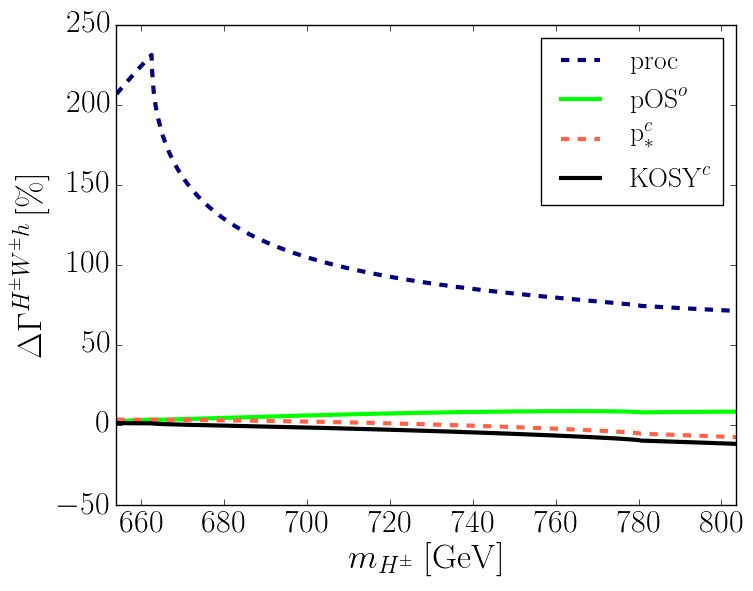
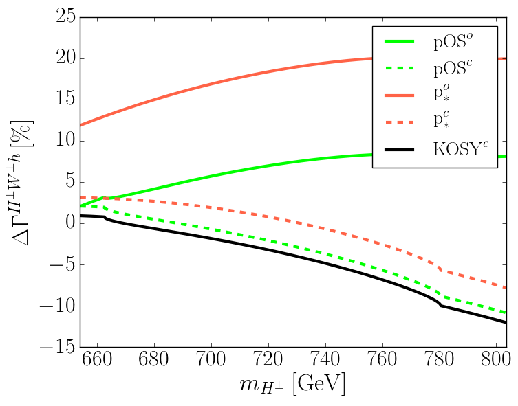
Figure 13: Relative NLO corrections to $H^{\pm}\to W^{\pm}h$ for various renormalization schemes as defined in Eq. (5.31), with the 2HDM parameters given by Scen2, Eq. (5.23); left: with, right: without the process-dependent renormalization.

Discarding the numerically unstable process-dependent scheme and the unphysical KOSY scheme, we can use the comparison of the results for $p_{\star}^{c}$ and $p_{\star}^{o}$ and the comparison of those for pOS^c and pOS^o to estimate the remaining theoretical uncertainty due to missing higher order corrections, based on a change of the renormalization scheme for $\beta$. In the same way we can estimate the uncertainty based on a variation of the renormalization scale by comparing the results for pOS^o and $p_{\star}^{o}$ or the results for pOS^c and p${}_{\star}^{c}$. In the investigated $m_{H^{\pm}}$ range from the lower to the upper end, the remaining uncertainty varies between 1% and 11%, when estimated from the scale change, and from close to 0 to 18%, when estimated from the change of the $\beta$ renormalization scheme. Note also that the results in the tadpole-pinched scheme, when evaluated at the OS scale, are less affected by a change of the renormalization scheme for $\delta\beta$ than in the $p_{\star}$ scheme. The renormalization of $\beta$ through the charged sector is less sensitive to the scale choice than $\delta\beta^{(2)}$, which uses the CP-odd sector, as can be inferred by comparing $p_{\star}^{c}$ with pOS^c on the one hand, and $p_{\star}^{o}$ and pOS^o on the other hand. Taking these as indicators for theoretical uncertainties, one might draw the conclusion that the pOS^c scheme would be the best choice here. Finally, we note that the kinks, which are independent of the renormalization scheme, are due to the thresholds in the following counterterms and parameter configurations

Kink	Kinematic point	Origin
1	$m_{H^{\pm}}(662.46\mbox{ GeV})=M_{H}(742.84\mbox{ GeV})-M_{W}$	$\delta Z_{H^{\pm}H^{\mp}},\delta Z_{G^{\pm}H^{\mp}}$
2	$m_{H^{\pm}}(780.51\mbox{ GeV})=M_{A}(700.13\mbox{ GeV})+M_{W}$	$\delta Z_{H^{\pm}H^{\mp}},\delta Z_{G^{\pm}H^{\mp}}$

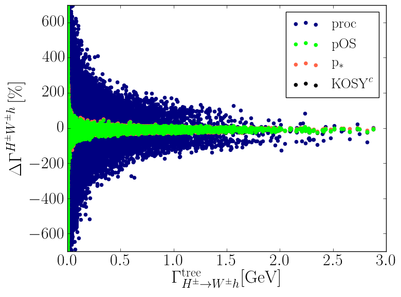
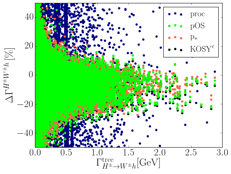
Figure 14: Scatter plots for the relative NLO corrections to $H^{\pm}\to W^{\pm}h$ for all parameter points passing the theoretical and experimental constraints as a function of the LO width; shown for various renormalization schemes: process-dependent (blue), pOS tadpole-pinched (green), $p_{\star}$ tadpole-pinched (red), KOSY^c (black). The right plot zooms into the central region.

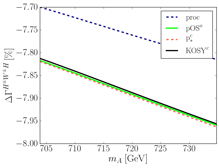
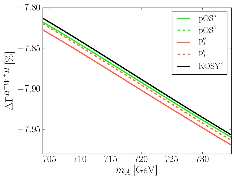
Figure 15: Relative NLO corrections to $H^{\pm}\to W^{\pm}H$ for various renormalization schemes, with the 2HDM parameters given by Scen3, Eq. (5.26); left: with, right: without the process-dependent renormalization. In the right plot the lines for KOSY^c and pOS^c lie on top of each other.

In Fig. 14 we show the relative NLO corrections for $H^{\pm}\to W^{\pm}h$ as a function of the LO width for all generated scenarios compatible with the applied theoretical and experimental constraints. The colours indicate the results for the process-dependent scheme, the $p_{\star}$ tadpole-pinched schemes, the OS tadpole-pinched schemes and the KOSY^c scheme. The plots demonstrate that the process-dependent renormalization in general leads to relative NLO corrections that are one to two orders of magnitude above those obtained in the other schemes, which yield corrections of typically a few percent up to 40%, as can be inferred from the right plot.

In Fig. 15 we show the relative NLO corrections for the process $H^{\pm}\to W^{\pm}H$ with the parameters given by Scen3, Eq. (5.26). In the plotted $m_{A}$ range the LO decay width, which does not depend on $m_{A}$, is given by $\Gamma^{\text{LO}}=4.0568$ GeV. In the left plot we have included the results for the process-dependent renormalization, for pOS^o, $p_{\star}^{c}$ and KOSY^c. The right plot includes all renormalization schemes but the process-dependent one. The relative corrections lie between about $-7.70$ to $-7.97$% in the investigated mass range. Altogether the results for all schemes lie very close to each other, with the process-dependent scheme deviating the most from the remaining schemes, although the difference in $\Delta\Gamma$ is of maximally 0.16% only. This behaviour can be understood by looking at the counterterm for the NLO process, Eq. (4.13). The contributions from the angular counterterms $\delta\alpha$ and $\delta\beta$ come with the factor $1/t_{\beta-\alpha}$, which is numerically very small in the SM-like limit $h\equiv H^{\text{SM}}$. Therefore any difference in the renormalization schemes for the angles will barely manifest itself in the total NLO corrections. The zoomed in region in Fig. 15 (right) again shows that the KOSY scheme is closer to pOS than to the other schemes and that the usage of the OS scale in $\delta\beta$ is less sensitive to a change of the renormalization scheme, while the renormalization of $\beta$ via the charged sector is less sensitive to a scale change than the one through the CP-odd sector.

5.3 The process $\Gamma(H\to ZZ)$ at NLO

We now turn to the discussion of the NLO corrections to the heavy Higgs boson decay into a pair of $Z$ bosons, $H\to ZZ$. The scenario we have chosen is given by

$$\begin{array}[]{llll}\mbox{\it\text@underline{Scen4:}}&\;m_{H^{\pm}}=659.16\mbox{ GeV}\,,&\;m_{H}=(690...809)\mbox{ GeV}\,,&\;m_{A}=705.44\mbox{ GeV}\,,\\ &\;\tan\beta=1.24\,,&\;\alpha=-0.61\,,&\;m_{12}^{2}=2.045\cdot 10^{5}\mbox{ GeV}^{2}\,.\end{array}$$ (5.34)

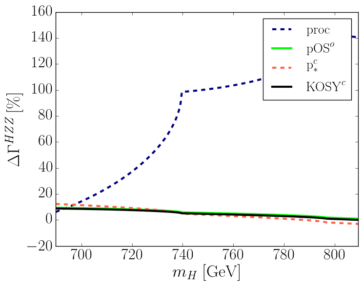
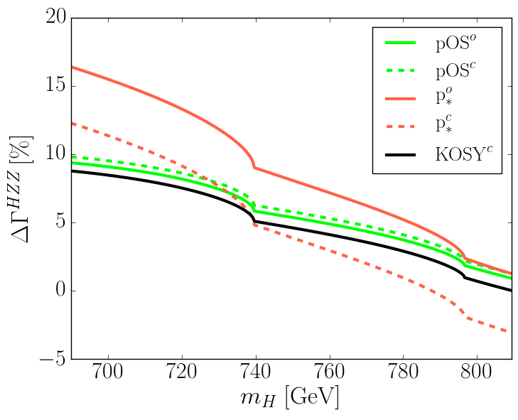
Figure 16: Relative NLO corrections to $H\to ZZ$ for various renormalization schemes, with the 2HDM parameters given by Scen4, Eq. (5.34); left: with, right: without the process-dependent renormalization.

In Fig. 16 we show the relative NLO corrections $\Delta\Gamma^{H\to ZZ}$ for the decay $H\to ZZ$ as a function of the heavier CP-even Higgs mass $m_{H}$ for different renormalization schemes. The LO width ranges from 0.2314 GeV to 0.3845 GeV in the plotted $m_{H}$ range. The kinks are due to

Kink	Kinematic point	Origin
1	$m_{H}(739.55\mbox{ GeV})=m_{H^{\pm}}(659.16\mbox{ GeV})+M_{W}$	$\delta Z_{HH},\delta Z_{hH}$
2	$m_{H}(796.63\mbox{ GeV})=m_{A}(705.44\mbox{ GeV})+M_{Z}$	$\delta Z_{HH},\delta Z_{hH}$

In the left plot the process-dependent renormalization is included. Additionally we show representatives for process-independent schemes, the pOS^o, the $p_{\star}^{c}$ and the KOSY^c scheme. Again the counterterm definition via tauonic heavy Higgs decays leads to much larger corrections than the other schemes. In the investigated mass range it can increase the LO decay width by more than a factor of two. The observed coincidence of the results for the process-independent and process-dependent renormalization schemes at $m_{H}=690$ GeV is accidental. The relative corrections in the process-dependent renormalization start to increase quickly again for different $m_{H}$ values. The NLO increase in the process-independent schemes, on the other hand, ranges from about -3 to 17% in the investigated parameter range. The right plot shows the same behaviour we have seen previously. The results in the KOSY and in the pOS scheme are closer to each other than to the $p_{\star}$ scheme. Furthermore, the change of the $\beta$ renormalization scheme affects the pOS scheme less than the $p_{\star}$ scheme and the $\beta$ renormalization through the charged sector is less sensitive to a change in the renormalization scale than the one through the CP-odd sector. Overall, in the investigated mass range, the theoretical uncertainty due to missing higher order corrections can be estimated to be of less than a percent to around 6% based on a scale change, and it ranges from the permille level to about 4% when estimated from the change of the $\beta$ renormalization scheme, discarding the numerically unstable process-dependent scheme.

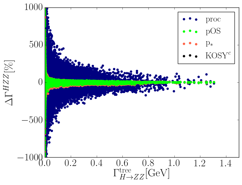
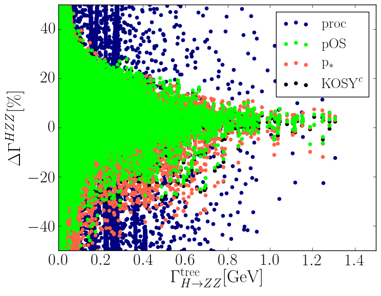
Figure 17: Scatter plots for the relative NLO corrections to $H\to ZZ$ for all parameter points passing the theoretical and experimental constraints as a function of the LO width; shown for various renormalization schemes: process-dependent (blue), pOS tadpole-pinched (green), $p_{\star}$ tadpole-pinched (red), KOSY (black). The right plot zooms into the central region.

Figure 17 shows the relative NLO corrections $\Delta\Gamma^{H\to ZZ}$ for $H\to ZZ$ as a function of the LO width for all generated scenarios compatible with the applied theoretical and experimental constraints. The colours indicate the results for the various renormalization schemes. The plots clearly demonstrate the numerical instability of the process-dependent renormalization, which exceeds the relative corrections in the other schemes by one to two orders of magnitudes. For the process-independent schemes the relative corrections are typically of the order of a few percent to 40%, discarding the region with small LO widths.

Altogether we conclude, that the choice of the KOSY scheme for the renormalization of the angular counterterms is precluded due to its manifest gauge dependence. The choice of the process-dependent scheme is not advisable, as it leads to very large relative NLO corrections. The process-independent tadpole-pinched schemes lead to results that are manifestly gauge-independent and numerically stable. Among these schemes the OS tadpole-pinched scheme turns out to be more stable when changing the $\beta$ renormalization scheme than the $p_{\star}$ scheme for our investigated scenarios.

6 Conclusions and Outlook

We have investigated the renormalization of the 2HDM with special focus on the mixing angles $\alpha$ and $\beta$ which diagonalize the Higgs mass matrices. These angles are highly relevant for the phenomenology of the Higgs bosons as they enter the Higgs boson couplings and therefore all Higgs observables. We have shown that if the tadpoles are treated in the more usual approach, which we called ’standard tadpole’, a process-independent definition of the angular counterterms leads to gauge-dependent decay amplitudes and thus to gauge-dependent physical observables. Therefore, the counterterms $\delta\alpha$ and $\delta\beta$ either have to be defined through a physical process, or the treatment of the tadpoles has to be changed. Following the ’alternative tadpole’ scheme as proposed in [29] allows for a manifestly gauge-independent definition of the masses and in particular of the mixing angles.

In this work we presented several distinct renormalization schemes and investigated their implications by applying them to the NLO EW corrections in the decays $H^{\pm}\to W^{\pm}h$, $H^{\pm}\to W^{\pm}H$ and $H\to ZZ$. It was explicitly shown that the scheme presented in [23] leads to gauge-dependent decay widths. This scheme applies the standard tadpole scheme and relates the angular counterterms to the off-diagonal wave function renormalization constants. By using the alternative tadpole scheme together with the modified Higgs self-energies obtained from the application of the pinch technique we introduced the ’tadpole-pinched’ scheme as a manifestly gauge-independent scheme for the angular counterterms. We furthermore investigated the process-dependent definition of $\delta\alpha$ and $\delta\beta$ through the decays $H\to\tau\tau$ and $A\to\tau\tau$, respectively. In this scheme the angular counterterms are gauge dependent when the standard tadpole scheme is applied, they are gauge independent in case the alternative tadpole scheme is used. For the investigated decay processes and scenarios, the process-dependent scheme turned out to lead to unnaturally large relative NLO corrections. Based on the investigated parameter sets and decay widths this leads us to the conclusion to propose the tadpole-pinched scheme as the renormalization scheme for the mixing angles that is at the same time process independent, gauge independent and numerically stable.

In order to complete the renormalization of the 2HDM, also the renormalization of the soft-breaking parameter $m_{12}^{2}$ has to be investigated. This parameter appears in the couplings of the Higgs self-interactions and hence impacts the Higgs-to-Higgs decay widths. The renormalization of $m_{12}^{2}$ and the phenomenological investigation of the implications of the higher order corrections for Higgs phenomenology will be the subject of a follow-up paper.

Acknowledgments

The authors acknowledge financial support from the DAAD project “PPP Portugal 2015” (ID: 57128671). Hanna Ziesche acknowledges financial support from the Graduiertenkolleg “GRK 1694: Elementarteilchenphysik bei höchster Energie und höchster Präzision”. We want to thank Marco Sampaio for kindly providing us with 2HDM data sets. We are grateful to Fawzi Boudjema, Thi Nhung Dao, Ayres Freitas, David Lopez-Val, Dominik Stöckinger and Georg Weiglein for helpful discussions. We want to thank Michael Spira and Augusto Barroso for useful comments.

Appendix

Appendix A The Tadpole Scheme in the 2HDM

In this section we will explain in detail the tadpole scheme, by applying it to the 2HDM, and show how to derive the relations for the mass counterterms and the wave function renormalization constants. We will furthermore derive which additional vertices have to be considered when performing explicit calculations in this scheme. At the end of this appendix, in A.2, we will give the complete list of rules for the application of the tadpole scheme.

A.1 Derivation of the Tadpole Scheme

We start by setting the notation and by presenting the standard scheme before we move on to the derivation of the tadpole scheme in the 2HDM.

A.1.1 Setting of the notation and tadpole renormalization

The expansion of the two Higgs doublets $\Phi_{1}$ and $\Phi_{2}$ about the VEVs, cf. Eq. (2.8), leads to the mass matrices that are obtained from the terms bilinear in the Higgs fields in the 2HDM potential. Due to CP- and charge conservation they decompose into $2\times 2$ matrices for the neutral CP-even, neutral CP-odd and charged Higgs sector, respectively. As we have seen in Sec. 2 the minimum conditions of the potential require the tree-level tadpole parameters $T_{1}$ and $T_{2}$ to vanish. At lowest order they are given by Eqs. (2.33) and (2.34). These tadpole conditions can be exploited to eliminate $m_{11}$ and $m_{22}$. Higher order corrections, however, lead to non-vanishing tadpole contributions that have to be taken into account. Applying Eqs. (2.33) and (2.34) we arrive at the following mass matrices

$$M_{\rho}^{2} =\begin{pmatrix}m_{12}^{2}\frac{v_{2}}{v_{1}}+\lambda_{1}v_{1}^{2}&&-m_{12}^{2}+\lambda_{345}v_{1}v_{2}\\ -m_{12}^{2}+\lambda_{345}v_{1}v_{2}&&m_{12}^{2}\frac{v_{1}}{v_{2}}+\lambda_{2}v_{2}^{2}\end{pmatrix}+\begin{pmatrix}\frac{T_{1}}{v_{1}}&&0\\ 0&&\frac{T_{2}}{v_{2}}\end{pmatrix}$$ (A.1)

$$M_{\eta}^{2} =\left(\frac{m_{12}^{2}}{v_{1}v_{2}}-\lambda_{5}\right)\begin{pmatrix}v_{2}^{2}&&-v_{1}v_{2}\\ -v_{1}v_{2}&&v_{1}^{2}\end{pmatrix}+\begin{pmatrix}\frac{T_{1}}{v_{1}}&&0\\ 0&&\frac{T_{2}}{v_{2}}\end{pmatrix}$$ (A.2)

$$M_{\phi^{\pm}}^{2} =\left(\frac{m_{12}^{2}}{v_{1}v_{2}}-\frac{\lambda_{4}+\lambda_{5}}{2}\right)\begin{pmatrix}v_{2}^{2}&&-v_{1}v_{2}\\ -v_{1}v_{2}&&v_{1}^{2}\end{pmatrix}+\begin{pmatrix}\frac{T_{1}}{v_{1}}&&0\\ 0&&\frac{T_{2}}{v_{2}}\end{pmatrix}~{}.$$ (A.3)

Here we have explicitly kept the tadpole parameters although they vanish at tree level. This helps us to keep track of their non-vanishing contributions at higher orders when performing the renormalization program. The mass matrices are diagonalized by the rotation matrices $R$ rotating the scalar fields from the gauge basis into the mass basis, cf. Eqs. (2.13)-(2.23),

$$D_{\rho}^{2} = R(\alpha)^{T}M_{\rho}^{2}R(\alpha)$$ (A.4)

$$D_{\eta}^{2} = R(\beta)^{T}M_{\eta}^{2}R(\beta)$$ (A.5)

$$D_{\phi^{\pm}}^{2} = R(\beta)^{T}M_{\phi^{\pm}}^{2}R(\beta)\;.$$ (A.6)

The scalar mass eigenstates with same quantum numbers, grouped into the doublets $(H,h)$, $(G^{0},A)$ and $(G^{\pm},H^{\pm})$, mix at higher orders. The wave function renormalization constants, introduced in Eqs. (3.26)-(3.40) for the three doublets, also develop non-vanishing mixing contributions and form $2\times 2$ matrices with off-diagonal elements. In the following we will use a generic notation and denote with $\phi_{1}$ and $\phi_{2}$ the two scalars of the same doublet. With this notation we then have for Eqs. (3.26)-(3.40)

$$\left(\begin{array}[]{c}\phi_{1}\\ \phi_{2}\end{array}\right)\to\sqrt{Z_{\phi}}\left(\begin{array}[]{c}\phi_{1}\\ \phi_{2}\end{array}\right)\approx\left(\mathbbm{1}_{2\times 2}+\frac{\delta Z_{\phi}}{2}\right)\left(\begin{array}[]{c}\phi_{1}\\ \phi_{2}\end{array}\right)\;,$$ (A.13)

with

$$\frac{\delta Z_{\phi}}{2}\equiv\left(\begin{array}[]{cc}\frac{\delta Z_{\phi_{1}\phi_{1}}}{2}&\frac{\delta Z_{\phi_{1}\phi_{2}}}{2}\\ \frac{\delta Z_{\phi_{2}\phi_{1}}}{2}&\frac{\delta Z_{\phi_{2}\phi_{2}}}{2}\end{array}\right)\;.$$ (A.16)

For the diagonal mass matrices, denoted from now on generically by $D_{\phi}^{2}$, we introduce the counterterm matrix $\delta D_{\phi}^{2}$, which is a symmetric $2\times 2$ matrix whose specific form will be determined below. With these definitions the renormalized self-energy $\hat{\Sigma}_{\phi}$ becomes

$$\begin{split}\hat{\Sigma}_{\phi}(p^{2})&\equiv\begin{pmatrix}\hat{\Sigma}_{\phi_{1}\phi_{1}}(p^{2})&&\hat{\Sigma}_{\phi_{1}\phi_{2}}(p^{2})\\ \hat{\Sigma}_{\phi_{2}\phi_{1}}(p^{2})&&\hat{\Sigma}_{\phi_{2}\phi_{2}}(p^{2})\end{pmatrix}\\ &=\Sigma_{\phi}(p^{2})-\delta D^{2}_{\phi}+\frac{\delta Z_{\phi}^{\dagger}}{2}\left(p^{2}\mathbbm{1}_{2\times 2}-D_{\phi}^{2}\right)+\left(p^{2}\mathbbm{1}_{2\times 2}-D_{\phi}^{2}\right)\frac{\delta Z_{\phi}}{2}~{}~{},\end{split}$$ (A.17)

The self-energy $\Sigma_{\phi}$ is a symmetric $2\times 2$ matrix containing the 1PI self-energies of the scalar doublet $(\phi_{1},\phi_{2})$. We require OS renormalization conditions for the scalar Higgs fields yielding the following conditions for the counterterm $\delta D_{\phi}^{2}$ and the wave function renormalization constants $\delta Z_{\phi}$, ($i=1,2$)

$$\mbox{Re}\left[\delta D_{\phi_{i}\phi_{i}}^{2}\right] = \mbox{Re}\left[\Sigma_{\phi_{i}\phi_{i}}(m_{\phi_{i}}^{2})\right]$$ (A.18)

$$\delta Z_{\phi_{i}\phi_{i}} = -\mbox{Re}\left[\frac{\partial Z_{\phi_{i}\phi_{i}(p^{2})}}{\partial p^{2}}\right]_{p^{2}=m_{\phi_{i}}^{2}}$$ (A.19)

$$\delta Z_{\phi_{i}\phi_{j}} = \frac{2}{m_{\phi_{i}}^{2}-m_{\phi_{j}}^{2}}\mbox{Re}\left[\Sigma_{\phi_{i}\phi_{j}}(m_{\phi_{j}}^{2})-\delta D^{2}_{\phi_{i}\phi_{j}}\right]\;,\qquad i\neq j\;.$$ (A.20)

So far we have not specified $\delta D_{\phi}^{2}$. Its exact form depends on the treatment of the tadpoles in the renormalization procedure and will be elaborated below. In order to guarantee the correct minimization conditions for the Higgs potential also at one-loop order, the tadpoles are renormalized as

$$\hat{T}_{i}=T_{i}-\delta T_{i}=0\;,\qquad i=1,2\;,$$ (A.21)

where $T_{1}$ and $T_{2}$ are the sum of all one-loop tadpole contributions to the fields $\rho_{1}$ and $\rho_{2}$, respectively, in the gauge basis. Applying the renormalization conditions we have for the tadpole counterterms the conditions

$$\delta T_{i}=T_{i}\;,\qquad i=1,2\;.$$ (A.22)

In the mass basis we have

$$\left(\begin{array}[]{c}\delta T_{1}\\ \delta T_{2}\end{array}\right)=R(\alpha)\left(\begin{array}[]{c}\delta T_{H}\\ \delta T_{h}\end{array}\right)=\left(\begin{array}[]{c}c_{\alpha}\delta T_{H}-s_{\alpha}T_{h}\\ s_{\alpha}\delta T_{H}+c_{\alpha}T_{h}\end{array}\right)\;,$$ (A.29)

and

$$\delta T_{H}=T_{H}\qquad\mbox{and}\qquad\delta T_{h}=T_{h}\;.$$ (A.30)

The renormalization conditions for the tadpoles are shown pictorially in Fig. 18.

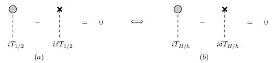
Figure 18: Renormalization condition for the tadpoles: (a) in the gauge basis, (b) in the mass basis.

A.1.2 Mass counterterms and wave function renormalization constants in the standard scheme

Regarding the renormalization of the masses, the bare mass of each particle in the 2HDM is split into a physical mass and a counterterm as specified in section 3. The VEVs $v_{1}$ and $v_{2}$, respectively $v$, are fixed at one-loop level such that their values in the tree-level mass relations for the scalars, derived by calculating explicitly Eqs. (A.4)-(A.6), lead to the OS physical masses at one-loop level. The shift from the bare parameter to the physical one-loop value is hence fully contained in the mass counterterms. In generic notation the diagonalized bare mass matrices read

$$\begin{split}D^{2}_{\phi,0}&=\begin{pmatrix}m_{\phi_{1},0}^{2}&&0\\ 0&&m_{\phi_{2},0}^{2}\end{pmatrix}+R_{\varphi}^{T}\begin{pmatrix}\frac{T_{1,0}}{v_{1}}&&0\\ 0&&\frac{T_{2,0}}{v_{2}}\end{pmatrix}R_{\varphi}\;\end{split}$$ (A.31)

where the subscript $0$ denotes the bare quantities and $\varphi=\alpha$ for the CP-even, $\varphi=\beta$ for the CP-odd and charged doublets, respectively. We have explicitly kept the bare tadpole parameters to keep track of their renormalization. Taking into account the renormalization of the tadpole parameters given in Eq. (A.22) we arrive at the NLO counterterm for the mass matrix

$$\begin{split}\delta D_{\phi}^{2}&\approx\begin{pmatrix}\delta m_{\phi_{1}}^{2}&&0\\ 0&&\delta m_{\phi_{2}}^{2}\end{pmatrix}+R_{\varphi}^{T}\begin{pmatrix}\frac{\delta T_{1}}{v_{1}}&&0\\ 0&&\frac{\delta T_{2}}{v_{2}}\end{pmatrix}R_{\varphi}\equiv\begin{pmatrix}\delta m_{\phi_{1}}^{2}&&0\\ 0&&\delta m_{\phi_{2}}^{2}\end{pmatrix}+\begin{pmatrix}\delta T_{\phi_{1}\phi_{1}}&&\delta T_{\phi_{1}\phi_{2}}\\ \delta T_{\phi_{1}\phi_{2}}&&\delta T_{\phi_{2}\phi_{2}}\end{pmatrix}\,,\end{split}$$ (A.32)

where we have consistently neglected all terms beyond NLO. The explicit form of the $T_{\phi_{i}\phi_{j}}$ is found by using Eq. (A.29) and applying the rotation to the mass basis,

$$\delta T_{HH} =\frac{c_{\alpha}^{3}s_{\beta}+s_{\alpha}^{3}c_{\beta}}{vs_{\beta}c_{\beta}}\delta T_{H}-\frac{s_{2\alpha}s_{\beta-\alpha}}{vs_{2\beta}}\delta T_{h}~{},$$ (A.33)

$$\delta T_{Hh} =-\frac{s_{2\alpha}s_{\beta-\alpha}}{vs_{2\beta}}\delta T_{H}+\frac{s_{2\alpha}c_{\beta-\alpha}}{vs_{2\beta}}\delta T_{h}~{},$$ (A.34)

$$\delta T_{hh} =\frac{s_{2\alpha}c_{\beta-\alpha}}{vs_{2\beta}}\delta T_{H}-\frac{s_{\alpha}^{3}s_{\beta}-c_{\alpha}^{3}c_{\beta}}{vs_{\beta}c_{\beta}}\delta T_{h}~{},$$ (A.35)

$$\delta T_{G^{0}G^{0}} =\frac{c_{\beta-\alpha}}{v}\delta T_{H}+\frac{s_{\beta-\alpha}}{v}\delta T_{h}~{},$$ (A.36)

$$\delta T_{G^{0}A} =-\frac{s_{\beta-\alpha}}{v}\delta T_{H}+\frac{c_{\beta-\alpha}}{v}\delta T_{h}~{},$$ (A.37)

$$\delta T_{AA} =\frac{c_{\alpha}s_{\beta}^{3}+s_{\alpha}c_{\beta}^{3}}{vs_{\beta}c_{\beta}}\delta T_{H}-\frac{s_{\alpha}s_{\beta}^{3}-c_{\alpha}c_{\beta}^{3}}{vs_{\beta}c_{\beta}}\delta T_{h}~{},$$ (A.38)

$$\delta T_{G^{+}G^{+}} =\frac{c_{\beta-\alpha}}{v}\delta T_{H}+\frac{s_{\beta-\alpha}}{v}\delta T_{h}~{},$$ (A.39)

$$\delta T_{G^{+}H^{+}} =-\frac{s_{\beta-\alpha}}{v}\delta T_{H}+\frac{c_{\beta-\alpha}}{v}\delta T_{h}~{},$$ (A.40)

$$\delta T_{H^{+}H^{+}} =\frac{c_{\alpha}s_{\beta}^{3}+s_{\alpha}c_{\beta}^{3}}{vs_{\beta}c_{\beta}}\delta T_{H}-\frac{s_{\alpha}s_{\beta}^{3}-c_{\alpha}c_{\beta}^{3}}{vs_{\beta}c_{\beta}}\delta T_{h}~{}.$$ (A.41)

Insertion of Eq. (A.32) in the renormalization conditions (A.18)-(A.20) we get the field strength renormalization constants and mass counterterms in the standard scheme

$$\delta m_{\phi_{i}}^{2} = \mbox{Re}\left[\Sigma_{\phi_{i}\phi_{i}}(m_{\phi_{i}}^{2})-\delta T_{\phi_{i}\phi_{i}}\right]$$ (A.42)

$$\delta Z_{\phi_{i}\phi_{i}} = -\mbox{Re}\left[\frac{\partial\Sigma_{\phi_{i}\phi_{i}}(p^{2})}{\partial p^{2}}\right]_{p^{2}=m_{\phi_{i}}^{2}}$$ (A.43)

$$\delta Z_{\phi_{i}\phi_{j}} = \frac{2}{m_{\phi_{i}}^{2}-m_{\phi_{j}}^{2}}\mbox{Re}\left[\Sigma_{\phi_{i}\phi_{j}}(m_{\phi_{j}}^{2})-\delta T_{\phi_{i}\phi_{j}}\right]\;,\qquad i\neq j\;.$$ (A.44)

These formulae can easily be generalized to the fermion and gauge boson sector. There, however, no tadpole counterterms will be involved, as they are not part of the tree-level mass relations. The counterterms introduced in Eqs. (A.42)-(A.44) are in general gauge dependent, which is not a problem, as long as all gauge dependencies cancel in physical observables. Since the renormalized masses must be gauge independent, the bare masses must be gauge dependent as well.

A.1.3 Mass counterterms and wave function renormalization constants in the tadpole scheme

We have seen that in the standard tadpole scheme the correct vacuum is reproduced by renormalizing the VEVs at higher orders accordingly. Derived from the gauge-dependent loop-corrected potential, the VEVs themselves are gauge dependent. The counterterms and the bare masses, that are given in terms of the VEVs therefore become gauge dependent, as the physical OS masses are gauge independent. In the tadpole scheme [29] the same renormalization conditions as given in Eq. (A.22), respectively in Eq. (A.30), are used. The crucial point, however, is the inclusion of the minimization conditions of the potential such that the mass and coupling counterterms can be defined in a gauge-independent way. This is achieved in the following way: In the alternative tadpole scheme the bare masses are expressed in terms of the tree-level VEVs. As the tree-level VEVs are gauge independent, the bare masses do not depend on the gauge choice either. In order to still reproduce the correct minimum at higher orders, the VEVs acquire a shift. This shift now affects the counterterms and not the bare masses, as the latter are expressed in terms of the tree-level VEVs. The gauge dependences related to the VEV shifts cancels those of the counterterms, so that the counterterms become gauge independent themselves. Together with the gauge-independent bare masses the OS renormalized masses are gauge independent as they should be. The VEVs are hence shifted when going from LO to NLO as

$$v_{1}\to v_{1}+\delta v_{1}\qquad\mbox{and}\qquad v_{2}\to v_{2}+\delta v_{2}\;.$$ (A.45)

We emphasize that $v_{1,2}$ represent the tree-level values of the VEVs. The shifts $\delta v_{1,2}$ are fixed by the minimization, that is, by the tadpole conditions. The tadpole parameters are given in terms of the VEVs, cf. Eqs. (2.33) and (2.34), so that a shift in the VEVs corresponds to a shift in the tadpole parameters. Note that we apply the term ’shift’ here in order to describe the changes of the parameters due to the VEV shifts, and to differ these from the counterterms for the chosen set of independent parameters.

The shifts in the VEVs are propagated into all parameters that depend on the VEVs. These shifts are determined as follows: $(i)$ Express the parameters in terms of $v_{1}$ and $v_{2}$. $(ii)$ Perform the shifts Eq. (A.45) of the VEVs. $(iii)$ Apply the tree-level relations between the VEVs and the various parameters to remove the redundant parameters $m_{11}^{2}$, $m_{22}^{2}$ and/or to simplify the expressions as convenient.

Thus by shifting and subsequently applying the tadpole conditions Eqs. (2.33) and (2.34) we obtain

$$T_{1}~{} \rightarrow~{}T_{1}+\bigg{(}m_{12}^{2}\frac{v_{2}}{v_{1}}+\lambda_{1}v_{1}^{2}\bigg{)}\delta v_{1}+\bigg{(}-m_{12}^{2}+\lambda_{345}v_{1}v_{2}\bigg{)}\delta v_{2}\equiv T_{1}+\delta T_{1}$$ (A.46)

$$T_{2}~{} \rightarrow~{}T_{2}+\bigg{(}-m_{12}^{2}+\lambda_{345}v_{1}v_{2}\bigg{)}\delta v_{1}+\bigg{(}m_{12}^{2}\frac{v_{1}}{v_{2}}+\lambda_{2}v_{2}^{2}\bigg{)}\delta v_{2}\equiv T_{2}+\delta T_{2}~{}.$$ (A.47)

Since the VEVs are determined order by order by applying the VEV shifts such that the tadpole conditions (2.33) and (2.34) hold we identify on the right-hand side of both equations the shift of the tadpole parameters induced by the shift of the VEVs with the counterterms $\delta T_{1}$ and $\delta T_{2}$. By comparing the coefficients of $\delta v_{1,2}$ in Eqs. (A.46) and (A.47) with the elements of the CP-even mass matrix given in Eq. (A.1) the following relation between the VEV shifts and the tadpole counterterms, that determine $\delta v_{1,2}$ can be derived

$$\begin{pmatrix}\delta T_{1}\\ \delta T_{2}\end{pmatrix}=\left.M^{2}_{\rho}\right|_{T_{i}=0}~{}\begin{pmatrix}\delta v_{1}\\ \delta v_{2}\end{pmatrix}~{}.$$ (A.48)

Rotation to the mass basis yields

$$\begin{pmatrix}\delta v_{H}\\ \delta v_{h}\end{pmatrix}=\begin{pmatrix}\frac{\delta T_{H}}{m_{H}^{2}}\\ \frac{\delta T_{h}}{m_{h}^{2}}\end{pmatrix}~{}.$$ (A.49)

By applying the renormalization condition depicted diagrammatically in Fig. 18, the shift can be interpreted as a connected tadpole diagram, containing the Higgs tadpole and its propagator at zero momentum transfer,

$$\delta v_{h_{i}}=\frac{-i}{m_{h_{i}}^{2}}i\delta T_{h_{i}}=\frac{-i}{m_{h_{i}}^{2}}~{}\mathord{\left(\rule{0.0pt}{30.11249pt}\right.\vbox{ \hbox{ \includegraphics[height=57.21375pt,trim=51.21495pt 34.1433pt 48.36967pt 28.45274pt,clip]{TadpoleDiagramHiggsBasis.pdf} } }\left.\rule{0.0pt}{30.11249pt}\right)=\left(\rule{0.0pt}{30.11249pt}\right.\vbox{ \hbox{ \includegraphics[height=57.21375pt,trim=49.79231pt 34.1433pt 43.81721pt 28.45274pt,clip]{TadpoleDiagramHiggsBasisWithVertex.pdf} } }\left.\rule{0.0pt}{30.11249pt}\right)}~{},$$ (A.50)

where $h_{i}\in\{H,h\}$ stands for the physical Higgs particles. For the consistent application of the tadpole scheme the VEV shifts have to be applied wherever the VEVs appear explicitly. As the calculation of the tadpole diagrams is usually performed in the mass basis, but the VEV shifts are introduced most conveniently in the gauge basis, we give the relation between the two bases,

$$\begin{pmatrix}\delta v_{1}\\ \delta v_{2}\end{pmatrix}=\begin{pmatrix}\frac{\delta T_{H}}{m_{H}^{2}}c_{\alpha}-\frac{\delta T_{h}}{m_{h}^{2}}s_{\alpha}\\ \frac{\delta T_{H}}{m_{H}^{2}}s_{\alpha}+\frac{\delta T_{h}}{m_{h}^{2}}c_{\alpha}\end{pmatrix}~{}.$$ (A.51)

For the illustration of the implications of the tadpole scheme we consider a specific example, namely the NLO effects of the VEV shifts on the CP-odd mass matrix given in Eq. (A.2). The application of the shifts requires the replacement of the tadpoles by $T_{i}+\delta T_{i}$, with the $\delta T_{i}$ given in Eqs. (A.46) and (A.47), and the replacement of all occurring VEVs by $v_{i}+\delta v_{i}$ so that we have

$$\begin{split}M_{\eta}^{2}~{}\rightarrow~{}&M_{\eta}^{2}+\begin{pmatrix}\frac{\delta T_{1}}{v_{1}}&&0\\ 0&&\frac{\delta T_{2}}{v_{2}}\end{pmatrix}+\left(\frac{m_{12}^{2}}{v_{1}v_{2}}-\lambda_{5}\right)\begin{pmatrix}2v_{2}\delta v_{2}&&-v_{1}\delta v_{2}-v_{2}\delta v_{1}\\ -v_{1}\delta v_{2}-v_{2}\delta v_{1}&&2v_{1}\delta v_{1}\end{pmatrix}\\ &-\frac{m_{12}^{2}}{v_{1}v_{2}}\left(\frac{\delta v_{1}}{v_{1}}+\frac{\delta v_{2}}{v_{2}}\right)\begin{pmatrix}v_{2}^{2}&&-v_{1}v_{2}\\ -v_{1}v_{2}&&v_{1}^{2}\end{pmatrix}+\begin{pmatrix}\frac{-T_{1}\delta v_{1}}{v_{1}^{2}}&&0\\ 0&&\frac{-T_{2}\delta v_{2}}{v_{2}^{2}}\end{pmatrix}~{}.\end{split}$$ (A.52)

Having applied the shifts, we can now use the tree-level relations again to eliminate the last matrix in Eq. (A.52), as the tadpole parameters vanish at tree-level. The rotation to the mass basis is performed by applying the rotation matrix $R(\beta)$ which is defined as the matrix diagonalizing the tree-level mass matrix $M_{\eta}^{2}$. We get

$$\begin{split}D_{\eta}~{}\rightarrow&~{}D_{\eta}+\begin{pmatrix}\delta T_{G^{0}G^{0}}&&\delta T_{G^{0}A}\\ \delta T_{G^{0}A}&&\delta T_{AA}\end{pmatrix}-\frac{\Lambda_{5}v}{s_{2\beta}}\left(s_{\beta}\delta v_{1}+c_{\beta}\delta v_{2}\right)\begin{pmatrix}0&&0\\ 0&&1\end{pmatrix}\\ &\hskip 2.84544pt+\frac{m_{A}^{2}}{v}\begin{pmatrix}0&&s_{\beta}\delta v_{1}-c_{\beta}\delta v_{2}\\ s_{\beta}\delta v_{1}-c_{\beta}\delta v_{2}&&2\left(c_{\beta}\delta v_{1}+s_{\beta}\delta v_{2}\right)\end{pmatrix}\\ &\equiv D_{\eta}+\begin{pmatrix}\Delta D_{G^{0}G^{0}}&&\Delta D_{G^{0}A}\\ \Delta D_{G^{0}A}&&\Delta D_{AA}\end{pmatrix}~{},\end{split}$$ (A.53)

where we applied the definition of $\Lambda_{5}$ Eq. (4.26) and the tree-level relation for the mass of the pseudoscalar [23, 12]

$$m_{A}^{2}=v^{2}\left(\frac{m_{12}^{2}}{v_{1}v_{2}}-\lambda_{5}\right)\;.$$ (A.54)

We furthermore applied the definition of the tadpole matrix in the mass basis, Eq. (A.32). In the last line we defined the terms $\Delta_{G^{0}G^{0}}$, $\Delta_{G^{0}A}$ and $\Delta_{AA}$ that contain all effects of the VEV shifts on the physical mass matrix $D_{\eta}$. These shifts can be further evaluated. In order to do so, we introduce the coupling constants for the trilinear Higgs couplings [23]

$$g_{HG^{0}G^{0}} = \frac{-c_{\beta-\alpha}m_{H}^{2}}{v}$$ (A.55)

$$g_{hG^{0}G^{0}} = \frac{-s_{\beta-\alpha}m_{h}^{2}}{v}$$ (A.56)

$$g_{HAA} = \frac{-1}{v}\left(c_{\beta-\alpha}(2m_{A}^{2}-m_{H}^{2})+\frac{s_{\alpha+\beta}}{s_{2\beta}}(2m_{H}^{2}-v^{2}\Lambda_{5})\right)$$ (A.57)

$$g_{hAA} = \frac{-1}{v}\left(s_{\beta-\alpha}(2m_{A}^{2}-m_{h}^{2})+\frac{c_{\alpha+\beta}}{s_{2\beta}}(2m_{h}^{2}-v^{2}\Lambda_{5})\right)$$ (A.58)

$$g_{HAG^{0}} = \frac{-s_{\beta-\alpha}}{v}(m_{A}^{2}-m_{H}^{2})$$ (A.59)

$$g_{hAG^{0}} = \frac{c_{\beta-\alpha}}{v}(m_{A}^{2}-m_{h}^{2})\;.$$ (A.60)

By using the explicit form of the tadpole counterterm $\delta T_{G^{0}G^{0}}$ given in Eq. (A.36) the vanishing Goldstone boson mass receives the shift contribution $\Delta D_{G^{0}G^{0}}$

$$\begin{split}\Delta D_{G^{0}G^{0}}&=\delta T_{G^{0}G^{0}}=i\frac{-ic_{\beta-\alpha}}{v}m_{H}^{2}\frac{-i}{m_{H}^{2}}i\delta T_{H}+i\frac{-is_{\beta-\alpha}}{v}m_{h}^{2}\frac{-i}{m_{h}^{2}}i\delta T_{h}\\ &=i\,(ig_{HG^{0}G^{0}})\,\left(\frac{-i}{m_{H}^{2}}\right)\,(i\delta T_{H})+i\,(ig_{hG^{0}G^{0}})\,\left(\frac{-i}{m_{H}^{2}}\right)\,(i\delta T_{h})\\ &=\mathord{i\left(\rule{0.0pt}{27.10124pt}\right.\vbox{ \hbox{ \includegraphics[height=57.21375pt,trim=29.59084pt 36.98857pt 26.31879pt 34.1433pt,clip]{VEVShiftResultG0G0HH.pdf} } }\left.\rule{0.0pt}{27.10124pt}\right)+i\left(\rule{0.0pt}{27.10124pt}\right.\vbox{ \hbox{ \includegraphics[height=57.21375pt,trim=29.59084pt 36.98857pt 26.31879pt 34.1433pt,clip]{VEVShiftResultG0G0h0.pdf} } }\left.\rule{0.0pt}{27.10124pt}\right)}~{}.\end{split}$$ (A.61)

In the second line we have used Eqs. (A.55) and (A.56). The last line is the diagrammatic representation of $\Delta T_{G^{0}G^{0}}$. It is given by two tadpole contributions from the CP-even Higgs bosons to the neutral Goldstone boson self-energy. Analogously we find for $\Delta D_{AA}$ by using Eqs. (A.38), (A.51), (A.57) and (A.58),

$$\begin{split}\Delta D_{AA}&=\delta T_{AA}-\frac{\Lambda_{5}v}{s_{2\beta}}\left(s_{\beta}\delta v_{1}+c_{\beta}v_{2}\right)+\frac{2m_{A^{0}}^{2}}{v}\left(c_{\beta}\delta v_{1}+s_{\beta}\delta v_{2}\right)\\ &=i\frac{-i}{v}\bigg{(}c_{\beta-\alpha}\left(2m_{A}^{2}-m_{H}^{2}\right)+\frac{s_{\alpha+\beta}}{s_{2\beta}}\left(2m_{H}^{2}-v^{2}\Lambda_{5}\right)\bigg{)}\frac{-i}{m_{H}^{2}}i\delta T_{H}\\ &\hskip 10.52737pt+i\frac{-i}{v}\bigg{(}s_{\beta-\alpha}\left(2m_{A}^{2}-m_{h}^{2}\right)+\frac{c_{\alpha+\beta}}{s_{2\beta}}\left(2m_{h}^{2}-v^{2}\Lambda_{5}\right)\bigg{)}\frac{-i}{m_{h}^{2}}i\delta T_{h}\\ &=i\,(ig_{HAA})\,\left(\frac{-i}{m_{H}^{2}}\right)\,(i\delta T_{H})+i\,(ig_{hAA})\,\left(\frac{-i}{m_{h}^{2}}\right)\,(i\delta T_{h})\\ &=\mathord{i\left(\rule{0.0pt}{27.10124pt}\right.\vbox{ \hbox{ \includegraphics[height=57.21375pt,trim=29.59084pt 36.98857pt 26.31879pt 34.1433pt,clip]{VEVShiftResultA0A0HH.pdf} } }\left.\rule{0.0pt}{27.10124pt}\right)+i\left(\rule{0.0pt}{27.10124pt}\right.\vbox{ \hbox{ \includegraphics[height=57.21375pt,trim=29.59084pt 36.98857pt 26.31879pt 34.1433pt,clip]{VEVShiftResultA0A0h0.pdf} } }\left.\rule{0.0pt}{27.10124pt}\right)}~{}.\end{split}$$ (A.62)

The last line again reproduces the diagrammatic representation of the shift. The shift is hence given by two CP-even tadpole contributions to the $A$ boson self-energy. The off-diagonal shift $\Delta D_{G^{0}A}$ finally can be cast into the form by applying Eqs. (A.37), (A.51), (A.59) and (A.60),

$$\begin{split}\Delta D_{G^{0}A}&=\delta T_{G^{0}A}+\frac{m_{A}^{2}}{v}\left(s_{\beta}\delta v_{1}-c_{\beta}\delta v_{2}\right)\\ &=i\frac{-is_{\beta-\alpha}}{v}\left(m_{A}^{2}-m_{H}^{2}\right)\frac{-i}{m_{H}^{2}}i\delta T_{H}+i\frac{ic_{\beta-\alpha}}{v}\left(m_{A}^{2}-m_{h}^{2}\right)\frac{-i}{m_{h}^{2}}i\delta T_{h}\\ &=i\,(ig_{HAG^{0}})\,\left(\frac{-i}{m_{H}^{2}}\right)\,(i\delta T_{H})+i\,(ig_{hAG^{0}})\,\left(\frac{-i}{m_{h}^{2}}\right)\,(i\delta T_{h})\\ &=\mathord{i\left(\rule{0.0pt}{27.10124pt}\right.\vbox{ \hbox{ \includegraphics[height=57.21375pt,trim=29.59084pt 36.98857pt 26.31879pt 34.1433pt,clip]{VEVShiftResultG0A0HH.pdf} } }\left.\rule{0.0pt}{27.10124pt}\right)+i\left(\rule{0.0pt}{27.10124pt}\right.\vbox{ \hbox{ \includegraphics[height=57.21375pt,trim=29.59084pt 36.98857pt 26.31879pt 34.1433pt,clip]{VEVShiftResultG0A0h0.pdf} } }\left.\rule{0.0pt}{27.10124pt}\right)}~{}.\end{split}$$ (A.63)

The diagrammatic representation in the last line reveals that the shift $\Delta G_{GA}$ consists of two CP-even tadpole contributions to the off-diagonal $G^{0}A$ self-energy. It is straightforward to derive the remaining shifts for the whole scalar sector. The total shift of the mass matrices, which is given by the shifts $\Delta D$ induced by the NLO shifts of the VEVs and by the mass counterterms, then reads

$$\delta D_{\phi}^{2}=\begin{pmatrix}\delta m_{\phi_{1}}^{2}&&0\\ 0&&\delta m_{\phi_{2}}^{2}\end{pmatrix}+\begin{pmatrix}\Delta D_{\phi_{1}\phi_{1}}&&\Delta D_{\phi_{1}\phi_{2}}\\ \Delta D_{\phi_{1}\phi_{2}}&&\Delta D_{\phi_{2}\phi_{2}}\end{pmatrix}~{},$$ (A.64)

with the explicit form of the additional mass shifts ($i=1,2$)

$$\Delta D_{\phi_{i}\phi_{j}}=\mathord{i\left(\rule{0.0pt}{27.10124pt}\right.\vbox{ \hbox{ \includegraphics[height=57.21375pt,trim=29.59084pt 36.98857pt 26.31879pt 34.1433pt,clip]{VEVShiftResultPhiPhioffHH.pdf} } }\left.\rule{0.0pt}{27.10124pt}\right)+i\left(\rule{0.0pt}{27.10124pt}\right.\vbox{ \hbox{ \includegraphics[height=57.21375pt,trim=29.59084pt 36.98857pt 26.31879pt 34.1433pt,clip]{VEVShiftResultPhiPhioffh0.pdf} } }\left.\rule{0.0pt}{27.10124pt}\right)}~{},$$ (A.65)

where $(\phi_{1},\phi_{2})$ refers to the pairs $(H,h)$, $(G^{0},A)$ and $(G^{\pm},H^{\pm})$, respectively. Equation (A.64) makes evident that in the tadpole scheme the tadpole counterterms $\delta T_{1}$ and $\delta T_{2}$ induced through the VEV shifts in Eqs. (A.46) and (A.47) have become part of the shift parameters $\Delta D_{\phi_{i}\phi_{j}}$ of the physical mass matrices of the scalar sector. They do not appear explicitly as counterterms, in contrast to the standard scheme where $\delta T_{1}$ and $\delta T_{2}$ were considered as counterterms being explicitly part of $\delta D_{\phi}^{2}$, cf. Eq. (A.32). Therefore, in the tadpole scheme, the tadpole counterterms Eqs. (A.33)-(A.41) do not belong to the definition of the mass counterterms and wave function renormalization constants. With the redefinition of the 1PI self-energy as

$$i\Sigma^{\text{tad}}_{\phi_{i}\phi_{j}}(p^{2})\equiv i\Sigma_{\phi_{i}\phi_{j}}(p^{2})-i\Delta D_{\phi_{i}\phi_{j}}$$ (A.66)

we obtain by inserting Eq. (A.64) in Eq. (A.17) the following form of the renormalized self-energy,

$$\hat{\Sigma}_{\phi}(p^{2})\equiv\Sigma^{\textrm{tad}}_{\phi}(p^{2})-\begin{pmatrix}\delta m_{\phi_{1}}^{2}&&0\\ 0&&\delta m_{\phi_{2}}^{2}\end{pmatrix}+\frac{\delta Z_{\phi}^{\dagger}}{2}\left(p^{2}\mathbbm{1}_{2\times 2}-D_{\phi}^{2}\right)+\left(p^{2}\mathbbm{1}_{2\times 2}-D_{\phi}^{2}\right)\frac{\delta Z_{\phi}}{2}~{}~{}.$$ (A.67)

And finally the counterterms and wave function renormalization constants in the tadpole scheme read

$$\delta m_{\phi_{i}}^{2} = \mbox{Re}\left[\Sigma^{\text{tad}}_{\phi_{i}\phi_{i}}(m_{\phi_{i}}^{2})\right]$$ (A.68)

$$\delta Z_{\phi_{i}\phi_{i}} = -\mbox{Re}\left[\frac{\partial\Sigma^{\text{tad}}_{\phi_{i}\phi_{i}}(p^{2})}{\partial p^{2}}\right]_{p^{2}=m_{\phi_{i}}^{2}}$$ (A.69)

$$\delta Z_{\phi_{i}\phi_{j}} = \frac{2}{m_{\phi_{i}}^{2}-m_{\phi_{j}}^{2}}\mbox{Re}\left[\Sigma^{\text{tad}}_{\phi_{i}\phi_{j}}(m_{\phi_{j}}^{2})\right]\;,\qquad\hskip 1.42271pti\neq j\;.$$ (A.70)

These results can be generalized to the gauge boson and fermion sectors. The application of the tadpole scheme hence requires a redefinition of the self-energies as depicted diagrammatically in Fig. 19. In the gauge and fermion sectors this implies that the tadpole diagrams of the scalar Higgs bosons that couple to the gauge boson and fermion, respectively, have to be included in their self-energy. Furthermore, in the scalar sector the tadpole counterterms drop out of the definition of the wave function renormalization constants and mass counterterms.

Figure 19: Modified self-energy $i\Sigma^{\textrm{tad}}(p^{2})$ in the tadpole scheme, consisting of all 1PI self-energy diagrams together with the one-loop tadpole diagrams, indicated by a gray blob.

The VEV shifts introduced in Eq. (A.45) also have implications for the coupling constants of the vertices. Let us consider the example of the Higgs $H$ coupling to a pair of $Z^{\mu}Z^{\nu}$ bosons. Defining the needed coupling constants through the Feynman rules

$$HZ^{\mu}Z^{\nu}: ig_{HZZ}g^{\mu\nu}$$ (A.71)

$$HHZ^{\mu}Z^{\nu}: ig_{HHZZ}g^{\mu\nu}\;,$$ (A.72)

we have

$$g_{HZZ} = \frac{g^{2}vc_{\beta-\alpha}}{2c_{W}^{2}}=\frac{g^{2}}{2c_{W}^{2}}(c_{\alpha}v_{1}+s_{\alpha}v_{2})$$ (A.73)

$$g_{HHZZ} = \frac{g^{2}}{2c_{W}^{2}}\;.$$ (A.74)

The shifts Eq. (A.45) introduce a shift in the coupling constants. In order to perform this shift consistently, the coupling constants must be expressed in terms of the VEVs $v_{1}$ and $v_{2}$. When doing so, care has to be taken, to differentiate between the angles $\alpha$ and $\beta$ in the sense of mixing angles and $\beta$ in the sense of the ratio of the VEVs, cf. Eq. (2.27), and $\alpha$ in the sense of the ratio of the 2HDM parameters given in Eq. (2.30). The VEV shifts only affect the latter two.

The quartic coupling obviously does not receive any shift, while $g_{HZZ}$ contains $\beta$ as ratio of the VEVs so that it receives a shift. The angle $\alpha$ is a mixing angle here. At NLO we therefore have to make the replacement

$$\begin{split}ig_{HZZ}~{}&\rightarrow~{}ig_{HZZ}+\frac{ig^{2}}{2c_{W}^{2}}(c_{\alpha}\delta v_{1}+s_{\alpha}\delta v_{2})\\ &=ig_{HZZ}+\frac{ig^{2}}{2c_{W}^{2}}\left[(c_{\alpha}^{2}+s_{\alpha}^{2})\frac{\delta T_{H}}{m_{H}^{2}}+(s_{\alpha}c_{\alpha}-s_{\alpha}c_{\alpha})\frac{\delta T_{h}}{m_{h}^{2}}\right]\\ &=ig_{HZZ}+ig_{HHZZ}\,\left(\frac{-i}{m_{H}^{2}}\right)\,i\delta T_{H}\\ &=ig_{HZZ}+\mathord{\left(\rule{0.0pt}{30.11249pt}\right.\vbox{ \hbox{ \includegraphics[height=56.20999pt,trim=20.77051pt 22.76219pt 8.53581pt 22.76219pt,clip]{VEVShiftResultVertex.pdf} } }\left.\rule{0.0pt}{30.11249pt}\right)_{\textrm{trunc}}}\\ &\equiv ig_{HZZ}^{\textrm{tad}}\;.\end{split}$$ (A.75)

The subscript ’trunc’ means that all Lorentz structure of the vector bosons as well as the Lorentz structure of the coupling has been suppressed here for simplicity. In the derivation of this equation we have used Eq. (A.51) and the explicit form of the quartic coupling constant, Eq. (A.74). The Feynman rule for the $HZZ$ vertex in the tadpole scheme is then given by

$$ig_{HZZ}^{\textrm{tad}}\,g^{\mu\nu}\;.$$ (A.76)

The above result can be generalized to the whole 2HDM. In the tadpole scheme additional virtual vertex corrections have to be taken into account that manifest themselves in form of tadpdole vertex diagrams. The rule to be applied here is, that every 2HDM trilinear vertex receives corrections if the resulting quartic coupling constant exists, that connects the original trilinear vertex to the CP-even Higgs, that is attached to the tadpole. In the case above the vertex $g_{HHZZ}$ exists, so that the vertex acquires a tadpole contribution with $H$, but not with $h$, as the vertex $g_{hHZZ}$ does not exist.

As last example we look at the coupling between $W^{\pm}_{\mu}$, $H^{\pm}(p^{\prime})$ and $h(p)$, where $p^{\prime}(p)$ denotes the outgoing (incoming) momentum of $H^{\pm}$ ($h$). The Feynman rule for the coupling is given by

$$W^{\pm}_{\mu}H^{\pm}h:\quad\mp i\,g_{W^{\pm}H^{\pm}h}\,(p+p^{\prime})_{\mu}\,,$$ (A.77)

with the coupling constant

$$g_{W^{\pm}H^{\pm}h}=\frac{gc_{\beta-\alpha}}{2}\;.$$ (A.78)

Both angles in this coupling are true mixing angles, so that no VEV shift has to be applied. Therefore the vertex does not change in the tadpole scheme. This is in accordance with the rule given above: There exists no vertex $g_{W^{\pm}H^{\pm}hh}$ nor $g_{W^{\pm}H^{\pm}hH}$ that could connect a tadpole with $h$ or $H$ to the trilinear vertex.

A.2 Rules for the Tadpole Scheme in the 2HDM

In this Appendix we summarize all rules of the tadpole scheme for the 2HDM at NLO. The general rules are:

Self-energies: The self-energies in the wave function renormalization constants and counterterms change such that they contain additional tadpole contributions: $\Sigma(p^{2})\to\Sigma^{\text{tad}}(p^{2})$.

Tadpole counterterms: The tadpole counterterms in the scalar sector vanish: $\delta T_{\phi_{i}\phi_{j}}\to 0$ ($i,j=1,2$).

Vertex corrections: In the virtual vertex corrections additional tadpole contributions have to be taken into account if the resulting coupling exists in the 2HDM.

Explicitly, this means that the following counterterms are the same in the standard and the alternative tadpole scheme:
Counterterms independent of the choice of the tadpole scheme:

$$\begin{array}[]{ll}\mbox{Tadpoles:}&\;\delta T_{H},\delta T_{h}\\[2.84544pt] \mbox{Gauge sector:}&\;\delta Z_{e},\delta g,\delta Z_{WW},\delta Z_{ZZ},\delta Z_{Z\gamma},\delta Z_{\gamma Z}\\[2.84544pt] \mbox{Fermion sector:}&\;\delta Z^{L}_{FF},\delta Z^{R}_{FF}\\[2.84544pt] \mbox{Scalar sector:}&\;\delta Z_{\phi_{i}\phi_{i}}\\[2.84544pt] \mbox{Vertices:}&\;\lambda_{FFS},\lambda_{FFV},\lambda_{SSV},\lambda_{SUU},\lambda_{UUV},\lambda_{VVV},\lambda_{VVVV}\end{array}$$ (A.84)

for all possible combinations of fermions $F$, gauge bosons $V$, ghosts $U$, scalars $S$ and $\phi_{i,j}\equiv H,h,G^{0},A,G^{\pm},H^{\pm}$ within the 2HDM.
The following counterterms and wave function renormalization constants depend on the choice of the tadpole scheme. We give the relations between the standard tadpole scheme, denoted by the superscript ’stand’, and the alternative tadpole scheme denoted by the superscript ’tad’. The subscript ’trunc’ means, that all spinors, all Lorentz structure of the vector bosons and the Lorentz structure of the coupling has been suppressed where applicable.
Tadpole-scheme-dependent counterterms:
Gauge sector:

$$(\delta m_{W}^{2})^{\textrm{tad}} =(\delta m_{W}^{2})^{\textrm{stand}}+i\mathord{\left(\rule{0.0pt}{26.09749pt}\right.\vbox{ \hbox{ \includegraphics[height=41.15375pt,trim=28.45274pt 56.9055pt 25.60747pt 29.59084pt,clip]{VEVShiftResultWWSelfEnergyHH.pdf} } }\left.\rule{0.0pt}{26.09749pt}\right)_{\textrm{trunc}}+i\left(\rule{0.0pt}{26.09749pt}\right.\vbox{ \hbox{ \includegraphics[height=41.15375pt,trim=28.45274pt 56.9055pt 25.60747pt 29.59084pt,clip]{VEVShiftResultWWSelfEnergyh0.pdf} } }\left.\rule{0.0pt}{26.09749pt}\right)_{\textrm{trunc}}}$$ (A.85)

$$(\delta m_{Z}^{2})^{\textrm{tad}} =(\delta m_{Z}^{2})^{\textrm{stand}}+i\mathord{\left(\rule{0.0pt}{26.09749pt}\right.\vbox{ \hbox{ \includegraphics[height=41.15375pt,trim=28.45274pt 56.9055pt 25.60747pt 29.59084pt,clip]{VEVShiftResultZZSelfEnergyHH.pdf} } }\left.\rule{0.0pt}{26.09749pt}\right)_{\textrm{trunc}}+i\left(\rule{0.0pt}{26.09749pt}\right.\vbox{ \hbox{ \includegraphics[height=41.15375pt,trim=28.45274pt 56.9055pt 25.60747pt 29.59084pt,clip]{VEVShiftResultZZSelfEnergyh0.pdf} } }\left.\rule{0.0pt}{26.09749pt}\right)_{\textrm{trunc}}}$$ (A.86)

Fermion sector:

$$(\delta m_{F})^{\textrm{tad}} =(\delta m_{F})^{\textrm{stand}}-i\mathord{\left(\rule{0.0pt}{26.09749pt}\right.\vbox{ \hbox{ \includegraphics[height=41.15375pt,trim=28.45274pt 56.9055pt 25.60747pt 29.59084pt,clip]{VEVShiftResultTauTauSelfEnergyHH.pdf} } }\left.\rule{0.0pt}{26.09749pt}\right)_{\textrm{trunc}}-i\left(\rule{0.0pt}{26.09749pt}\right.\vbox{ \hbox{ \includegraphics[height=41.15375pt,trim=28.45274pt 56.9055pt 25.60747pt 29.59084pt,clip]{VEVShiftResultTauTauSelfEnergyh0.pdf} } }\left.\rule{0.0pt}{26.09749pt}\right)_{\textrm{trunc}}}$$ (A.87)

Scalar sector:

$$(\delta m_{\phi_{i}})^{\textrm{tad}} =(\delta m_{\phi_{i}})^{\textrm{stand}}+\delta T_{\phi_{i}\phi_{i}}-i\mathord{\left(\rule{0.0pt}{26.09749pt}\right.\vbox{ \hbox{ \includegraphics[height=61.22874pt,trim=28.45274pt 39.83385pt 25.60747pt 29.59084pt,clip]{VEVShiftResultPhiPhiHH.pdf} } }\left.\rule{0.0pt}{26.09749pt}\right)_{\textrm{trunc}}-i\left(\rule{0.0pt}{26.09749pt}\right.\vbox{ \hbox{ \includegraphics[height=61.22874pt,trim=28.45274pt 39.83385pt 25.60747pt 29.59084pt,clip]{VEVShiftResultPhiPhih0.pdf} } }\left.\rule{0.0pt}{26.09749pt}\right)_{\textrm{trunc}}}$$ (A.88)

for all possible combinations of $\phi_{i,j}\equiv H,h,A,H^{\pm}$.

$$(\delta Z_{\phi_{i}\phi_{j}})^{\textrm{tad}} =(\delta Z_{\phi_{i}\phi_{j}})^{\textrm{stand}}$$ (A.89)

$$+\frac{2}{m_{\phi_{i}}^{2}-m_{\phi_{j}}^{2}}\left[\delta T_{\phi_{i}\phi_{j}}-i\mathord{\left(\rule{0.0pt}{26.09749pt}\right.\vbox{ \hbox{ \includegraphics[height=61.22874pt,trim=28.45274pt 39.83385pt 25.60747pt 29.59084pt,clip]{VEVShiftResultPhiPhioffHH.pdf} } }\left.\rule{0.0pt}{26.09749pt}\right)_{\textrm{trunc}}-i\left(\rule{0.0pt}{26.09749pt}\right.\vbox{ \hbox{ \includegraphics[height=61.22874pt,trim=28.45274pt 39.83385pt 25.60747pt 29.59084pt,clip]{VEVShiftResultPhiPhioffh0.pdf} } }\left.\rule{0.0pt}{26.09749pt}\right)_{\textrm{trunc}}}\right]~{},$$

where $\phi_{i}\neq\phi_{j}$.

We encounter additional contributions to the vertices when changing from the standard to the tadpole scheme. Here below, the $g$ denote the coupling constants, i.e. we have suppressed the Lorentz structure of the vertex where applicable.

Triple scalar vertices:

$$ig_{\phi_{i}\phi_{j}\phi_{k}}~{}\rightarrow~{}ig_{\phi_{i}\phi_{j}\phi_{k}}+\mathord{\left(\rule{0.0pt}{30.11249pt}\right.\vbox{ \hbox{ \includegraphics[height=56.20999pt,trim=20.77051pt 22.76219pt 8.53581pt 22.76219pt,clip]{VEVShiftResultVertexTripleScalarHH.pdf} } }\left.\rule{0.0pt}{30.11249pt}\right)_{\textrm{trunc}}+\left(\rule{0.0pt}{30.11249pt}\right.\vbox{ \hbox{ \includegraphics[height=56.20999pt,trim=20.77051pt 22.76219pt 8.53581pt 22.76219pt,clip]{VEVShiftResultVertexTripleScalarh0.pdf} } }\left.\rule{0.0pt}{30.11249pt}\right)_{\textrm{trunc}}}$$ (A.90)

for all scalars $\phi_{i,j,k}\equiv H,h,G^{0},A,G^{\pm},H^{\pm}$, wherever the resulting quartic couplings $\lambda_{\phi_{i}\phi_{j}\phi_{k}h}$ and $\lambda_{\phi_{i}\phi_{j}\phi_{k}H}$ exist in the 2HDM.

Scalar-vector-vector vertices:

$$ig_{\phi_{i}V_{j}V_{k}}~{}\rightarrow~{}ig_{\phi_{i}V_{j}V_{k}}+\mathord{\left(\rule{0.0pt}{30.11249pt}\right.\vbox{ \hbox{ \includegraphics[height=56.20999pt,trim=20.77051pt 22.76219pt 8.53581pt 22.76219pt,clip]{VEVShiftResultVertexScalarVectorVectorHH.pdf} } }\left.\rule{0.0pt}{30.11249pt}\right)_{\textrm{trunc}}+\left(\rule{0.0pt}{30.11249pt}\right.\vbox{ \hbox{ \includegraphics[height=56.20999pt,trim=20.77051pt 22.76219pt 8.53581pt 22.76219pt,clip]{VEVShiftResultVertexScalarVectorVectorh0.pdf} } }\left.\rule{0.0pt}{30.11249pt}\right)_{\textrm{trunc}}}$$ (A.91)

for all scalars $\phi_{i,j,k}\equiv H,h,G^{0},A,G^{\pm},H^{\pm}$, and gauge bosons $V_{j,k}\equiv\gamma,Z,W^{\pm}$, wherever the resulting quartic couplings $\lambda_{\phi_{i}V_{j}V_{k}h}$ and $\lambda_{\phi_{i}V_{j}V_{k}H}$ exist in the 2HDM.

References

• [1] ATLAS Collaboration, G. Aad et al., Phys.Lett. B716, 1 (2012), 1207.7214.
• [2] CMS Collaboration, S. Chatrchyan et al., Phys.Lett. B716, 30 (2012), 1207.7235.
• [3] CMS, V. Khachatryan et al., Phys. Rev. D92, 012004 (2015), 1411.3441.
• [4] ATLAS, G. Aad et al., Eur. Phys. J. C75, 476 (2015), 1506.05669.
• [5] CMS, V. Khachatryan et al., Eur. Phys. J. C75, 212 (2015), 1412.8662.
• [6] ATLAS, G. Aad et al., Eur. Phys. J. C76, 6 (2016), 1507.04548.
• [7] J. F. Gunion, H. E. Haber, G. L. Kane, and S. Dawson, Front.Phys. 80, 1 (2000).
• [8] S. P. Martin, Adv.Ser.Direct.High Energy Phys. 21, 1 (2010), hep-ph/9709356.
• [9] S. Dawson, p. 261 (1997), hep-ph/9712464.
• [10] A. Djouadi, Phys.Rept. 459, 1 (2008), hep-ph/0503173.
• [11] T. D. Lee, Phys. Rev. D8, 1226 (1973).
• [12] G. C. Branco et al., Phys. Rept. 516, 1 (2012), 1106.0034.
• [13] ATLAS Collaboration, CERN Report No. ATLAS-CONF-2015-081, 2015 (unpublished).
• [14] CMS Collaboration, CERN Report No. CMS-PAS-EXO-15-004, 2015 (unpublished).
• [15] R. Barbieri, L. J. Hall, and V. S. Rychkov, Phys.Rev. D74, 015007 (2006), hep-ph/0603188.
• [16] L. Lopez Honorez, E. Nezri, J. F. Oliver, and M. H. Tytgat, JCAP 0702, 028 (2007), hep-ph/0612275.
• [17] Q.-H. Cao, E. Ma, and G. Rajasekaran, Phys.Rev. D76, 095011 (2007), 0708.2939.
• [18] E. M. Dolle and S. Su, Phys.Rev. D80, 055012 (2009), 0906.1609.
• [19] M. Gustafsson, S. Rydbeck, L. Lopez-Honorez, and E. Lundstrom, Phys.Rev. D86, 075019 (2012), 1206.6316.
• [20] A. Arhrib, Y.-L. S. Tsai, Q. Yuan, and T.-C. Yuan, JCAP 1406, 030 (2014), 1310.0358.
• [21] A. Ilnicka, M. Krawczyk, and T. Robens, (2015), 1508.01671.
• [22] R. Santos and A. Barroso, Phys. Rev. D56, 5366 (1997), hep-ph/9701257.
• [23] S. Kanemura, Y. Okada, E. Senaha, and C. P. Yuan, Phys. Rev. D70, 115002 (2004), hep-ph/0408364.
• [24] S. Kanemura, M. Kikuchi, and K. Yagyu, Nucl. Phys. B896, 80 (2015), 1502.07716.
• [25] A. Freitas and D. Stockinger, Phys. Rev. D66, 095014 (2002), hep-ph/0205281.
• [26] A. Denner, Fortsch. Phys. 41, 307 (1993), 0709.1075.
• [27] G. ’t Hooft and M. Veltman, Nucl.Phys. B153, 365 (1979).
• [28] G. Passarino and M. J. G. Veltman, Nucl. Phys. B160, 151 (1979).
• [29] J. Fleischer and F. Jegerlehner, Phys. Rev. D23, 2001 (1981).
• [30] P. Gambino and P. A. Grassi, Phys. Rev. D62, 076002 (2000), hep-ph/9907254.
• [31] D. Pierce and A. Papadopoulos, Phys. Rev. D47, 222 (1993), hep-ph/9206257.
• [32] A. Dabelstein, Z.Phys. C67, 495 (1995), hep-ph/9409375.
• [33] P. H. Chankowski, S. Pokorski, and J. Rosiek, Nucl.Phys. B423, 437 (1994), hep-ph/9303309.
• [34] J. A. Coarasa Perez, D. Garcia, J. Guasch, R. A. Jimenez, and J. Sola, Eur. Phys. J. C2, 373 (1998), hep-ph/9607485.
• [35] L.-Y. Shan, Eur. Phys. J. C12, 113 (2000), hep-ph/9807456.
• [36] S. Heinemeyer, W. Hollik, and G. Weiglein, Phys. Rept. 425, 265 (2006), hep-ph/0412214.
• [37] J. Fujimoto et al., Phys. Rev. D75, 113002 (2007).
• [38] N. Baro and F. Boudjema, Phys. Rev. D80, 076010 (2009), 0906.1665.
• [39] N. Baro, F. Boudjema, and A. Semenov, Phys. Rev. D78, 115003 (2008), 0807.4668.
• [40] Y. Yamada, Phys. Lett. B530, 174 (2002), hep-ph/0112251.
• [41] Y. Yamada, Phys. Rev. D64, 036008 (2001), hep-ph/0103046.
• [42] J. R. Espinosa and Y. Yamada, Phys. Rev. D67, 036003 (2003), hep-ph/0207351.
• [43] L. F. Abbott, Nucl. Phys. B185, 189 (1981).
• [44] L. F. Abbott, Acta Phys. Polon. B13, 33 (1982).
• [45] H. Kluberg-Stern and J. B. Zuber, Phys. Rev. D12, 482 (1975).
• [46] H. Kluberg-Stern and J. B. Zuber, Phys. Rev. D12, 3159 (1975).
• [47] D. G. Boulware, Phys. Rev. D23, 389 (1981).
• [48] C. F. Hart, Phys. Rev. D28, 1993 (1983).
• [49] A. Denner, G. Weiglein, and S. Dittmaier, Nucl. Phys. B440, 95 (1995), hep-ph/9410338.
• [50] A. Denner, G. Weiglein, and S. Dittmaier, Phys. Lett. B333, 420 (1994), hep-ph/9406204.
• [51] D. Binosi, J. Phys. G30, 1021 (2004), hep-ph/0401182.
• [52] D. Binosi and J. Papavassiliou, Phys. Rept. 479, 1 (2009), 0909.2536.
• [53] J. M. Cornwall and J. Papavassiliou, Phys. Rev. D40, 3474 (1989).
• [54] J. Papavassiliou, Phys. Rev. D41, 3179 (1990).
• [55] J. Papavassiliou, Phys. Rev. D50, 5958 (1994), hep-ph/9406258.
• [56] G. Degrassi and A. Sirlin, Phys. Rev. D46, 3104 (1992).
• [57] F. Bojarski, G. Chalons, D. Lopez-Val, and T. Robens, JHEP 02, 147 (2016), 1511.08120.
• [58] R. Santos, A. Barroso, and L. Brucher, Phys. Lett. B391, 429 (1997), hep-ph/9608376.
• [59] K. E. Williams, H. Rzehak, and G. Weiglein, Eur. Phys. J. C71, 1669 (2011), 1103.1335.
• [60] D. A. Ross and J. C. Taylor, Nucl. Phys. B51, 125 (1973), [Erratum: Nucl. Phys.B58,643(1973)].
• [61] L. Baulieu, Phys. Rept. 129, 1 (1985).
• [62] J. Kublbeck, M. Bohm, and A. Denner, Comput. Phys. Commun. 60, 165 (1990).
• [63] T. Hahn, Comput. Phys. Commun. 140, 418 (2001), hep-ph/0012260.
• [64] R. Mertig, M. Bohm, and A. Denner, Comput. Phys. Commun. 64, 345 (1991).
• [65] T. Hahn and M. Perez-Victoria, Comput. Phys. Commun. 118, 153 (1999), hep-ph/9807565.
• [66] G. ’t Hooft and M. J. G. Veltman, Nucl. Phys. B44, 189 (1972).
• [67] C. G. Bollini and J. J. Giambiagi, Nuovo Cim. B12, 20 (1972).
• [68] Particle Data Group, K. A. Olive et al., Chin. Phys. C38, 090001 (2014).
• [69] A. Denner et al., LHCHXSWG-INT-2015-006 (2015).
• [70] LHC Higgs Cross Section Working Group, https://twiki.cern.ch/twiki/bin/view/LHCPhysics/ LHCHXSWG .
• [71] LHC Higgs Cross Section Working Group, S. Dittmaier et al., (2011), 1101.0593.
• [72] ATLAS, CMS, G. Aad et al., Phys. Rev. Lett. 114, 191803 (2015), 1503.07589.
• [73] R. Lorenz, Master Thesis, 2015, Karlsruhe Institute of Technology (2015).
• [74] R. Coimbra, M. O. P. Sampaio, and R. Santos, Eur. Phys. J. C73, 2428 (2013), 1301.2599.
• [75] A. Barroso, P. M. Ferreira, I. P. Ivanov, and R. Santos, JHEP 06, 045 (2013), 1303.5098.
• [76] N. G. Deshpande and E. Ma, Phys. Rev. D18, 2574 (1978).
• [77] S. Kanemura, T. Kubota, and E. Takasugi, Phys. Lett. B313, 155 (1993), hep-ph/9303263.
• [78] A. G. Akeroyd, A. Arhrib, and E.-M. Naimi, Phys. Lett. B490, 119 (2000), hep-ph/0006035.
• [79] M. E. Peskin and T. Takeuchi, Phys. Rev. D46, 381 (1992).
• [80] C. D. Froggatt, R. G. Moorhouse, and I. G. Knowles, Phys. Rev. D 45, 2471 (1992).
• [81] W. Grimus, L. Lavoura, O. M. Ogreid, and P. Osland, Nucl. Phys. B801, 81 (2008), 0802.4353.
• [82] H. E. Haber and D. O’Neil, Phys. Rev. D83, 055017 (2011), 1011.6188.
• [83] Tevatron Electroweak Working Group, CDF, DELPHI, SLD Electroweak and Heavy Flavour Groups, ALEPH, LEP Electroweak Working Group, SLD, OPAL, D0, L3, L. E. W. Group, (2010), 1012.2367.
• [84] M. Baak et al., Eur. Phys. J. C72, 2003 (2012), 1107.0975.
• [85] M. Baak et al., Eur. Phys. J. C72, 2205 (2012), 1209.2716.
• [86] F. Mahmoudi and O. Stal, Phys. Rev. D81, 035016 (2010), 0907.1791.
• [87] O. Deschamps et al., Phys. Rev. D82, 073012 (2010), 0907.5135.
• [88] T. Hermann, M. Misiak, and M. Steinhauser, JHEP 11, 036 (2012), 1208.2788.
• [89] A. Denner, R. J. Guth, W. Hollik, and J. H. Kuhn, Z. Phys. C51, 695 (1991).
• [90] A. K. Grant, Phys. Rev. D51, 207 (1995), hep-ph/9410267.
• [91] H. E. Haber and H. E. Logan, Phys. Rev. D62, 015011 (2000), hep-ph/9909335.
• [92] A. Freitas and Y.-C. Huang, JHEP 08, 050 (2012), 1205.0299, [Erratum: JHEP10,044(2013)].
• [93] M. Misiak et al., Phys. Rev. Lett. 114, 221801 (2015), 1503.01789.
• [94] LEP, DELPHI, OPAL, ALEPH, L3, G. Abbiendi et al., Eur. Phys. J. C73, 2463 (2013), 1301.6065.
• [95] ATLAS, G. Aad et al., JHEP 03, 088 (2015), 1412.6663.
• [96] CMS, V. Khachatryan et al., JHEP 11, 018 (2015), 1508.07774.
• [97] ATLAS, G. Aad et al., JHEP 03, 127 (2016), 1512.03704.
• [98] R. V. Harlander, S. Liebler, and H. Mantler, Comput. Phys. Commun. 184, 1605 (2013), 1212.3249.
• [99] A. Djouadi, J. Kalinowski, and M. Spira, Comput. Phys. Commun. 108, 56 (1998), hep-ph/9704448.
• [100] R. Harlander, M. Muhlleitner, J. Rathsman, M. Spira, and O. Stal, (2013), 1312.5571.
• [101] P. Bechtle, O. Brein, S. Heinemeyer, G. Weiglein, and K. E. Williams, Comput. Phys. Commun. 181, 138 (2010), 0811.4169.
• [102] P. Bechtle, O. Brein, S. Heinemeyer, G. Weiglein, and K. E. Williams, Comput. Phys. Commun. 182, 2605 (2011), 1102.1898.
• [103] P. Bechtle et al., Eur. Phys. J. C74, 2693 (2014), 1311.0055.
• [104] P. Bechtle, S. Heinemeyer, O. Stal, T. Stefaniak, and G. Weiglein, Eur. Phys. J. C74, 2711 (2014), 1305.1933.
• [105] P. M. Ferreira, R. Guedes, M. O. P. Sampaio, and R. Santos, JHEP 12, 067 (2014), 1409.6723.
• [106] M. Krause, Master Thesis, 2016, Karlsruhe Institute of Technology (2016).