The JCMT Gould Belt Survey: Evidence for radiative heating and contamination in the W40 complex.

Abstract

We present SCUBA-2 450 $\micron$ and 850 $\micron$ observations of the W40 complex in the Serpens-Aquila region as part of the James Clerk Maxwell Telescope (JCMT) Gould Belt Survey (GBS) of nearby star-forming regions. We investigate radiative heating by constructing temperature maps from the ratio of SCUBA-2 fluxes using a fixed dust opacity spectral index, $\beta$ = 1.8, and a beam convolution kernel to achieve a common 14.8^′′ resolution. We identify 82 clumps ranging between 10 and 36 K with a mean temperature of 20$\pm$3 K. Clump temperature is strongly correlated with proximity to the external OB association and there is no evidence that the embedded protostars significantly heat the dust. We identify 31 clumps that have cores with densities greater than 10⁵cm^-3. Thirteen of these cores contain embedded Class 0/I protostars. Many cores are associated with bright-rimmed clouds seen in Herschel 70 $\micron$ images. From JCMT HARP observations of the ¹²CO 3–2 line, we find contamination of the 850 $\micron$ band of up to 20 per cent. We investigate the free-free contribution to SCUBA-2 bands from large-scale and ultracompact H ii regions using archival VLA data and find the contribution is limited to individual stars, accounting for 9 per cent of flux per beam at 450 $\micron$ or 12 per cent at 850 $\micron$ in these cases. We conclude that radiative heating has potentially influenced the formation of stars in the Dust Arc sub-region, favouring Jeans stable clouds in the warm east and fragmentation in the cool west.

1 Introduction

Understanding the impact of heating, via feedback, is of vital importance for the wider inquiry into what mechanisms govern the behaviour of molecular clouds (Jeans, 1902). Feedback occurs, via internal mechanisms, from radiative heating by the stellar photosphere and accretion luminosity (Calvet & Gullbring, 1998) of young stellar objects (YSOs). Molecular outflows and shocks (Davis et al., 1999) may also radiatively heat a cloud to a lesser extent. External sources of heating include photons produced by stars, which can drive strong stellar winds (Canto et al., 1984; Ziener & Eislöffel, 1999; Malbet et al., 2007) and H ii regions (Koenig et al., 2008; Deharveng et al., 2012), as well as the interstellar radiation field (ISRF; Mathis, Mezger & Panagia, 1983; Shirley, Evans, Rawlings & Gregersen, 2000; Shirley, Evans & Rawlings, 2002). Simulations, including those by Bate (2009), Offner et al. (2009), and Hennebelle & Chabrier (2011), have suggested that internal radiative feedback can suppress cloud fragmentation, leading to higher mass star-formation, whereas observations by Rumble et al. (2015) provided evidence that external heating can influence the evolution of star-forming clouds.

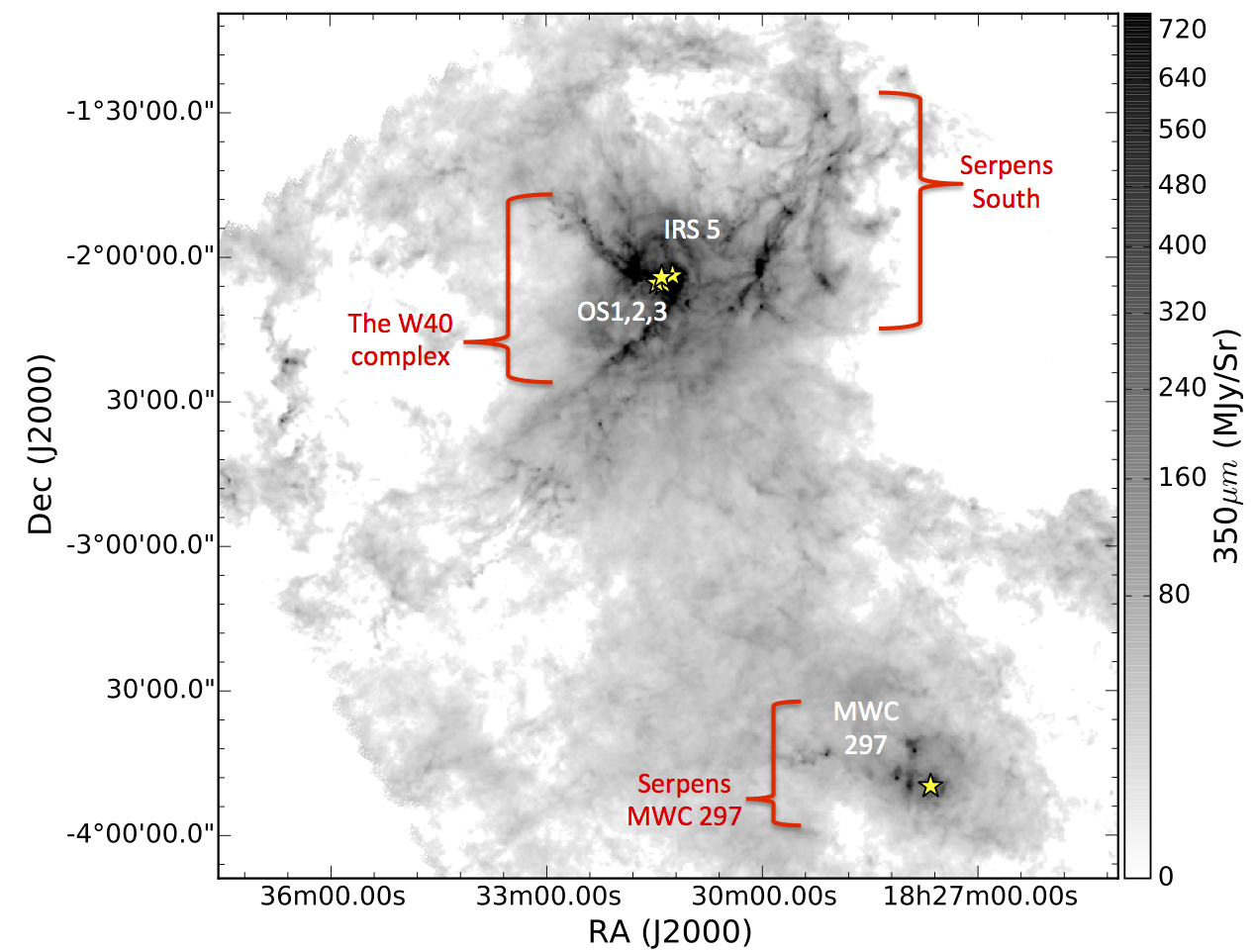
Figure 1: Herschel 350 $\micron$ map of the Aquila Rift including the W40 complex, Serpens South and Serpens MWC 297. OB stars are marked with yellow crosses and labelled Bontemps et al. (2010).

Fluxes of cool YSOs observed at longer wavelengths may appear on the Rayleigh-Jeans tail of the continuum, where temperature cannot be calculated. Use of the shorter SCUBA-2 450 $\micron$ band allows for dust temperatures up to 35 K to be reliably calculated for an opacity modified grey-body model fit to a flux ratio. Flux ratios have been calculated by Mitchell et al. (2001), Reid & Wilson (2005), Hatchell et al. (2013), and Rumble et al. (2015) for Submillimetre Common-User Bolometer Array (SCUBA, Cunningham et al. 1994) and SCUBA-2 (Holland et al., 2013) bands. The flux ratio method does not compromise on the high resolution of the JCMT (14.6^′′) but does introduce an inherent degeneracy between temperature and the dust opacity index, $\beta$, requiring an assumption in either case (Shetty et al., 2015).

This study uses data from the JCMT Gould Belt Survey (GBS) of nearby star-forming regions (Ward-Thompson et al., 2007) to measure dust temperatures. The full survey maps all major low- and intermediate-mass star-forming regions within 0.5 kpc observable from the JCMT with the continuum bolometer array SCUBA-2 (Holland et al. 2013). The JCMT GBS provides some of the most sensitive maps of star-forming regions where $A_{V}>3$ with a target sensitivity of 3 mJy beam^-1 at 850 $\micron$ and 12 mJy beam^-1 at 450 $\micron$. The 9.8 ^′′ (450 $\micron$) and 14.6 ^′′ (850 $\micron$; Dempsey et al., 2013) resolutions of the JCMT allow for detailed study of structures such as filaments and protostellar envelopes down to the Jeans length.

We focus on the W40 complex (presented in Figure 1). The neighbouring Serpens South filament is thought to be part of the Aquila Rift ($255\pm 55\hbox{ pc}$ Straižys et al. 2003). Bontemps et al. (2010) and Maury et al. (2011) therefore conclude a physical association with Serpens South on account of proximity. However, Kuhn et al. (2010) calculates a distance of 600 pc via fits to the X-ray luminosity function. Shuping et al. (2012) construct SEDs from IR data of bright objects in the W40 complex and estimate a distance between 455 pc and 536 pc. We use a mean distance based on these calculations of $500\pm 50\hbox{ pc}$, following Radhakrishnan et al. (1972), and Mallick et al. (2013). The W40 complex is therefore assumed to be spatially separated from the Serpens South region (Straižys et al., 2003; Gutermuth et al., 2008).

The W40 complex is a site of high-mass star-formation associated with a cold molecular cloud (Dobashi et al., 2005) and includes a blistered H ii region (Westerhout, 1958) powered by an OB association (Zeilik & Lada, 1978; Smith et al., 1985). The OB association is comprised of IRS/OS1a (O9.5), IRS/OS2b (B4) and IRS/OS3a (B3) and an associated stellar cluster of pre-main-sequence (PMS) stars that are detected in the X-ray by Kuhn et al. (2010). OS1aS is the primary ionising source of the H ii region that was detected in the radio via free-free emission (Vallee & MacLeod, 1991). The OB association drives the formation of the larger nebulosity Sh2-64 (Sharpless, 1959). The W40 complex is detected in the submillimetre by the Herschel Space Telescope (André et al., 2010; Men’shchikov et al., 2010; Könyves et al., 2010; Bontemps et al., 2010; Könyves et al., 2015) with three significant filaments (W40-N, W40-S and the Dust Arc). Rodney & Reipurth (2008) present a further review of the W40 complex.

In addition to the SCUBA-2 data for Aquila, we make use of JCMT HARP ¹²CO 3–2 line emission observed over an area 30 times larger than that observed by van der Wiel et al. (2014), and remove the contribution from the CO line emission to the 850 $\micron$ SCUBA-2 maps. We also make use of archival VLA 21 cm data (45^′′ resolution; Condon & Kaplan 1998) and assess the impact of the larger scale free-free emission contribution to the SCUBA-2 bands. Furthermore, we use archival AUI/NRAO 3.6 cm data alongside the Rodríguez et al. (2010) 3.6 cm catalogue of compact radio sources to assess the impact of smaller scale free-free emission contribution to the SCUBA-2 bands. Finally, we complement our findings with 70 $\micron$ observations from the Herschel archive.

This paper is structured as follows. In Section 2, we describe the observations of the Serpens-Aquila region with SCUBA-2 and HARP. In Sections 3 and 4, we describe the methods by which the contributions of CO line and free-free continuum emission was removed from SCUBA-2 observations. In Section 5, we apply our method for producing temperature maps. In Section 6, we identify clumps from SCUBA-2 data and calculate their properties. In Section 7, we discuss the evidence for radiative feedback influencing the evolution of clumps and the formation of stars in the W40 complex.

2 Observations and Data Reduction

2.1 SCUBA-2

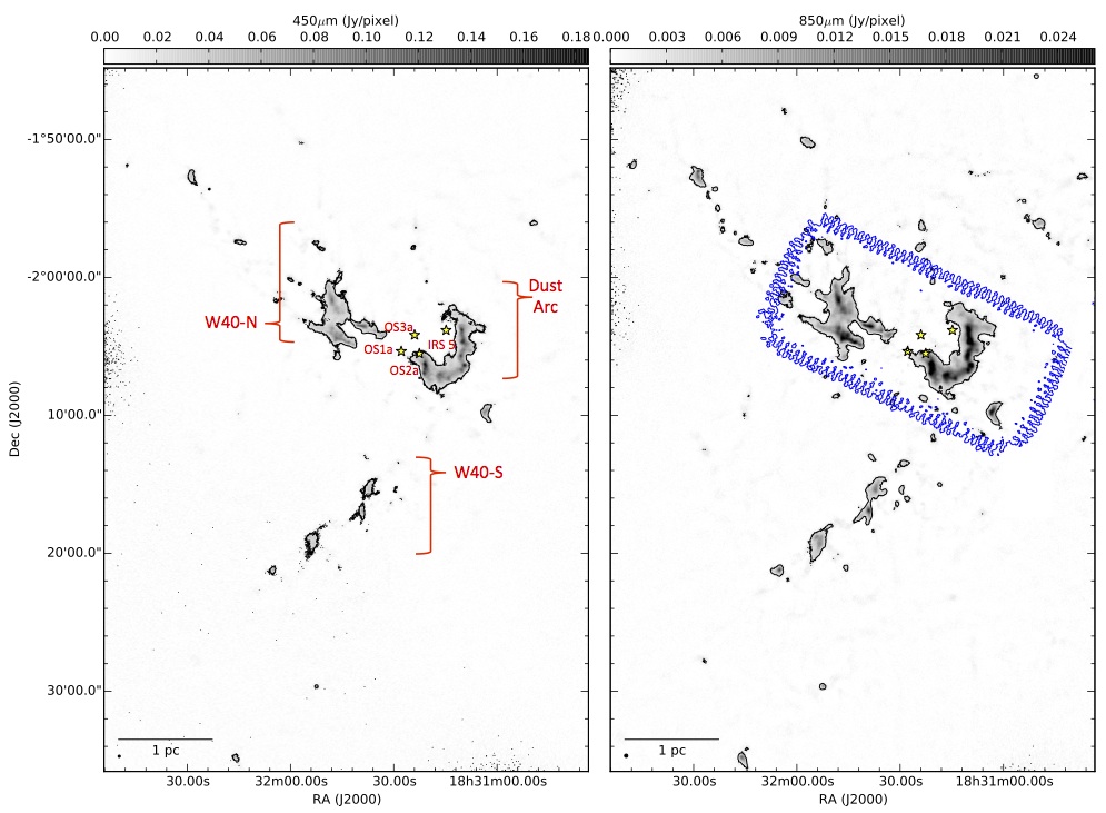
Figure 2: SCUBA-2 450 $\micron$ (left) and 850 $\micron$ (right) data. The SCUBA-2 850 $\micron$ data have had contaminating CO emission covering an 6^′43^′′ $\times$17^′54^′′  area removed (region outlined in blue, see Section 3.1 for more details). The resulting maps have been further filtered to remove structure above 4^′ in size (see Section 2.1). The contours show 5 $\sigma$ levels in both cases: levels are at 0.0173 Jy/ 2^′′ pixels and 0.0025 Jy/ 3^′′ pixels at 450 $\micron$ and 850 $\micron$ respectively.

Aquila was observed with SCUBA-2 (Holland et al., 2013) between the 21st of April and 5th of July 2012 as part of the JCMT GBS MJLSG33 SCUBA-2 Serpens Campaign. Four separate fully sampled 30^′ diameter circular continuum observations (PONG1800 mapping mode, Kackley et al. 2010) were taken simultaneously at 850 $\micron$ and 450 $\micron$, and subsequently combined into mosaics. The beam sizes in the two bands are 9.8 ^′′ (450 $\micron$) and 14.6 ^′′ (850 $\micron$). The 450 and 850 $\micron$ maps for the entire Aquila W40 / Serpens South area covered by SCUBA-2 are shown in Appendix A (Figure 22) along with the data reduction masks and variance maps. The spatially-filtered 450 and 850 $\micron$ mosaics for the W40 region are shown in Figure 2; the 850µm emission also has CO contamination removed (see Sect. 3). The dates, central positions and weather conditions of the observations are listed in Table 1.

Table 1: SCUBA-2 observations of Aquila

PONG	RA Dec	# of	Weather	Observation dates	Mean standard deviation
	(J2000)	Obs.	band(s)		(Jy per pixel)
NE	18:31:34.6 -01:54:05.30	4	1	21st, 23rd April, 3rd May 2012	4.7$\times$10-4
NW	18:29:30.6 -01:47:30.30	4	1, 2	3rd, 4th, 5th May 2012	4.5$\times$10-4
SE	18:32:13.8 -02:24:12.30	6	1, 2, 3	8th May, 10th, 11th June, 5th July 2012	4.0$\times$10-4
SW	18:30:09.8 -02:17:37.30	4	1	7th, 8th, 18th May 2012	4.6$\times$10-4

The data were reduced as part of the GBS Legacy Release 1 (LR1, Mairs et al. 2015) using an iterative map-making technique (makemap in smurf, Chapin et al. 2013), and gridded to a 3^′′ pixel grid at 850 $\micron$ and a 2^′′ pixel grid at 450 $\micron$. The iterations were halted when the map pixels, on average, changed by $<$0.1 per cent of the estimated map rms noise. The initial reductions of each individual scan were coadded to form a mosaic from which a signal-to-noise ratio (SNR) mask was produced for each region. Masks were selected to include regions of emission in the automask reductions with SNRs higher than 3 with no additional smoothing.

The final mosaic was produced from a second reduction using this mask to define areas of emission. Detection of emission structure and calibration accuracy (see below) are robust within the masked regions and are uncertain outside of the masked region (Mairs et al., 2015).

A spatial filter of 600^′′ was used in the reduction, which means that within appropriately sized masks flux recovery is robust for sources with Gaussian Full Width Half Maximum (FWHM) sizes less than 2.5^′. Sources between 2.5^′ and 7.5^′ in extent will be detected, but both the flux and the size are underestimated because Fourier components with scales greater than 5^′ are removed by the filtering process. Detection of sources larger than 7.5^′ is dependent on the mask used for reduction.

The data were initially calibrated in units of pW and are converted to Jy per pixel using Flux Conversion Factors (FCFs) derived by Dempsey et al. (2013) as FCF_arcsec = 2.34 $\pm$ 0.08 pW^-1 arcsec^-2 and 4.71 $\pm$ 0.5 Jy pW^-1 arcsec^-2 at 850 $\micron$ and 450 $\micron$ respectively. The calibration uncertainties on the standard FCFs are 3% at 850 $\micron$ and 11% at 450 $\micron$. For ratios and temperatures derived from these data, it is not the uncertainties at each wavelength but the uncertainties on the calibration ratio that matter. Due to correlations between the 450 $\micron$ and 850 $\micron$ FCF measurements, the errors do not propagate simply. For a single scan, the calibration ratio is FCF₄₅₀/FCF₈₅₀ = 2.04 $\pm$ 0.49 (J. Dempsey, priv. comm.). The SCUBA-2 mosaics for Aquila were made with at least four scans per region. Assuming these to be randomly drawn from the distribution of calibration ratios, the uncertainty on the ratio reduces to 2.04 $\pm$ 0.25 or a calibration uncertainty of 12.5%.

The PONG scan pattern leads to lower noise in the map centre and overlap regions, while data reduction and emission artefacts can lead to small variations in the noise over the whole map. Due to varying conditions over the observing periods, the noise levels are not consistent across the mosaic. Typical noise levels are 3.5 mJy/pix or 0.50 mJy/pix per 2^′′or 3^′′ pixel at 450 $\micron$ and 850 $\micron$, respectively.

After masking, we found that the SCUBA-2 data reduction process was removing less large scale structure at 450 $\micron$, relative to 850 $\micron$. As a result, a significant number of pixels had flux ratio values that would lead to unphysically high temperatures (defined as ratios higher than 9.5 which correspond to temperatures greater than 50 K). Flux ratio and temperature are related through the ‘temperature equation’ that is given below in Section 5. The details of flux ratio preparation are given in Appendix A. To ameliorate this problem, a further spatial filter was applied to the data, the details of which are provided in Appendix B. In summary, a scale size of 4^′ at both 450 and 850 $\micron$ was found to be the optimal solution and the SCUBA-2 maps were filtered accordingly.

2.2 HARP

Archival HARP ${}^{12}\textrm{CO}$ 3–2 data (van der Wiel et al., 2014) confirms the presence of red- and blue-shifted gas in the Dust Arc (Figure 2) but coverage is limited to a 2^′ $\times$ 2^′ region centred on the local peak of the submilimetre emission, and therefore we commissioned an extended survey of the W40 complex in ${}^{12}\textrm{CO}$ 3–2 that included the whole of the Dust Arc and W40-N, as presented in Figures 2 and 3 upper. Subsequent to our observations, Shimoikura et al. (2015) published maps of the W40 complex from Atacama Submillimeter Telescope Experiment (ASTE) observations in ${}^{12}\textrm{CO}$ 3–2 and HCO⁺ 4–3 with a similar coverage, but at a lower effective resolution of 22^′′ compared to the JCMT (14.6^′′).

Aquila was observed with HARP (Heterodyne Array Receiver Programme, Buckle et al. 2009) on the 4th of July 2015 as part of the M15AI31“active star-formation in the W40 complex” proposal. The main beam efficiency, $\eta_{\mathrm{MB}}$, taken from the JCMT efficiency archive is 0.61 at 345 GHz. Two sets of four basket-weaving scan maps were observed over an approximately 7^′$\times$18^′ area (position angle = 65${\degr}$) at 345.796 GHz to observe the ¹²CO 3–2 line. A sensitivity of 0.3 K was achieved on 1 km s^-1 velocity channels in weather Grade 4 ($\tau_{225}$ = 0.16). Maps were referenced against an off-source position at RA(J2000) = 18:33:29.0, Dec.(J2000) = -02:03:45.4, which had been selected as being free of any significant CO emission in the Dame et al. (2001) CO Galactic Plane Survey.

The observed cube has two distinct velocity components at 5 and 10 km s^-1 that are consistent with the observations of Zeilik & Lada (1978) and Shimoikura et al. (2015). A third component at 7 km s^-1 is detected in observations of the HCO⁺ 4–3 line. Shimoikura et al. (2015) suggest that ¹²CO 3–2 is heavily affected by self-absorption by this third cloud component, making a full analysis of velocity structure of the W40 complex challenging.

The data were first reduced using the smurf makecube technique (Jenness et al., 2015). An integrated intensity map, corrected for main beam efficiency, was produced by collapsing along the entire velocity range and subsequently run through the SCUBA-2 data reduction pipeline with the effect of filtering out scales larger than 5^′ as well as regridding to 3^′′ pixels. Figure 3 upper presents the reduced ¹²CO 3–2 integrated intensity map for the W40 complex.

The bulk of the ¹²CO 3–2 gas coexists with the brightest dust observed by SCUBA-2, but a bright filament of ¹²CO 3–2 emission is observed between W40-N and the Dust Arc with no corresponding SCUBA-2 emission (see Figure 3, upper panel). This is interpreted by Shimoikura et al. (2015) as low density gas that has been swept up and heated by the expanding H ii region.

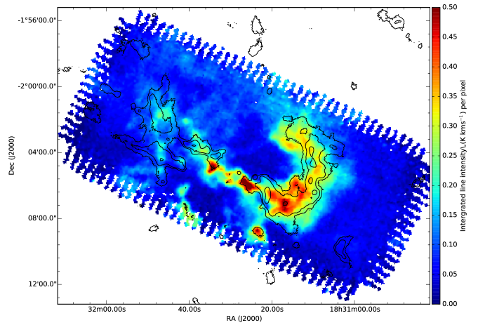
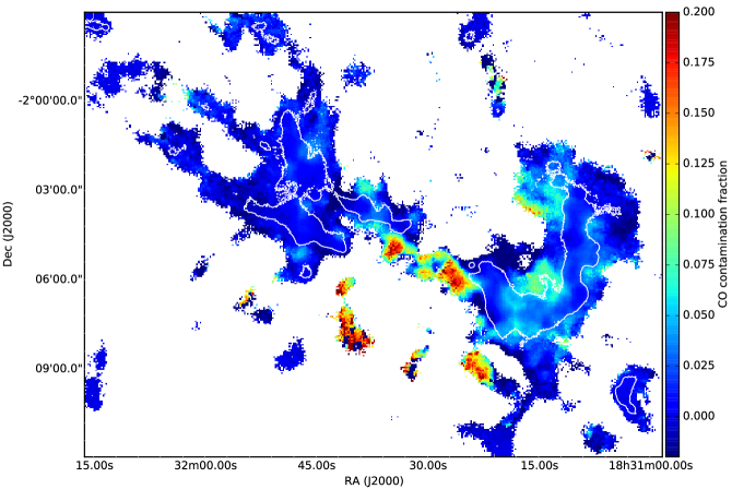
Figure 3: Upper ¹²CO 3–2 integrated intensity map over the entire range (from -90 to +100 km s^-1) of the central region of the W40 complex. Contours show SCUBA-2 850 $\micron$ emission at the 5 $\sigma$, 15 $\sigma$ and 50 $\sigma$ levels. Lower the fraction of SCUBA-2 850 $\micron$ that can be attributed to ${}^{12}\textrm{CO}$ 3–2 345 GHz line emission. The SCUBA-2 data are masked at 3 $\sigma$ and the 5 $\sigma$ level is shown by the white contour.

2.3 YSO catalogues

Alongside a known population of one late O star, three B stars and two Herbig AeBe stars (Smith et al., 1985; Shuping et al., 2012) there is a young stellar cluster (Kuhn et al., 2010; Kuhn et al., 2015). The Spitzer Space Telescope legacy programme ‘Gould’s Belt: star-formation in the solar neighbourhood’ (SGBS, PID: 30574, Dunham et al. 2015) provides specific locations and properties of the YSOs. This catalogue is incomplete due to saturation of Spitzer at the heart of the OB association and may be contaminated by the IR bright clouds in the nebulosity. Additional catalogues are required to verify and complete the YSO population.

We create a new, conservative YSO catalogue of SGBS objects (Dunham et al., 2015) matched with Mallick et al. (2013)’s Spitzer catalogue, Maury et al. (2011)’s MAMBO catalogue of submillimetre objects, and Kuhn et al. (2010)’s X-ray catalogue. The SGBS objects are matched with the Mallick et al. (2013) sources, except where the SGBS is saturated around the H ii region. In those cases, we turn to the Kuhn et al. (2010) catalogue of K-band excess objects as a proxy list of Class II and III objects. By matching the Mallick et al. (2013) and Kuhn et al. (2010) sources, IR bright clouds which may have been misidentified as sources can be excised. These two sub-catalogues are subsequently merged, with any duplicates removed. The Maury et al. (2011) catalogue of submillimetre objects, and the Rodríguez et al. (2010) and Ortiz-León et al. (2015) radio YSOs are added separately and are not examined for IR contamination. We include a classification where it is reported by an author; otherwise Class is determined by IR dust spectral index, $\alpha$, between 2-24 $\micron$ (based on the boundaries of $\alpha_{\mathrm{IR}}$ = 0.3, -0.3 and -1.6 for Class 0/I, FS, II and III, respectively, as summarised by Evans et al. 2009). In lieu of a comprehensive YSO catalogue covering the whole of the W40 complex, our composite catalogue, presented in Table 2, allows a conservative analysis to be made of the global YSO distribution.

Table 2: Our composite YSO catalogue, produced from the combined SGBS (Dunham et al. 2015), the Mallick et al. (2013) Spitzer catalogue, the Maury et al. (2011) MAMBO catalogue, the Kuhn etal. (2010) X-ray catalogue, and the Rodr$\mathrm{\acute{i}}$guez etal. (2010) catalogue of radio YSOs. The full catalogue is available online.

Namea	YSO	$\alpha$b	Tbolb
	class	(2-24µm)	(K)
2MASS18303312-0207055	II	-0.78	1400
2MASS18303314-0220581	II	-1.93	1700
2MASS18303324-0211258	II	-0.48	950
2MASS18303509-0208564	II	-0.86	1200
2MASS18303590-0206492	II	-1.45	1700

${a}$ - 2MASS or CXO name where available. RA Dec coordinates (J2000) where not.
${b}$ - T_bol and $\alpha$ values as published by Dunham et al. (2015).

3 CO contamination of SCUBA-2 850 $\micron$

We use our HARP 345.796 GHz observations of the ¹²CO 3–2 line emission to assess the impact of CO emission on the 850 $\micron$ band, which it is known to contaminate (Gordon, 1995).

In other GBS regions, Davis et al. (2000) and Tothill et al. (2002) observed CO contamination of SCUBA data of up to 10% whilst Hatchell & Dunham (2009) have found contamination up to 20%. Johnstone et al. (2003), Drabek et al. (2012), and Sadavoy et al. (2013) record a minority of cases where CO emission dominates the dust emission (up to 90%) in SCUBA-2 observations, with these regions hosting substantial molecular outflows in addition to ambient molecular gas within the clouds.

Given that CO contamination affects the 850 $\micron$ band but not the 450 $\micron$ band, an assessment of ¹²CO 3–2 line emission is vital for an accurate assessment of dust temperature with unaccounted CO emission producing artificially lower ratios and cooler temperatures (Equation 3, see Section 5 below). We use Drabek et al. (2012)’s method by which CO line integrated intensities can be converted into 850 $\micron$ flux densities and directly subtracted from SCUBA-2 data.

3.1 Contamination results

Integrated intensity maps of ${}^{12}\textrm{CO}$ 3–2 emission are subtracted from the original SCUBA-2 850 $\micron$ maps using a joint data reduction process before a 4^′ filter is applied following the method outlined in Appendix C. The fraction of SCUBA-2 emission that can be accounted for by ${}^{12}\textrm{CO}$ 3–2 line emission is presented in Figure 3 (lower panel). Contamination in W40-N is minimal with levels up to 5%. The Dust Arc has significant contamination at a level of 10%, reaching up to 20% in some locations.

Figure 4 shows the distribution of flux ratios (see Equation 3 and the method given in Appendix A) with and without CO contamination contributing to the 850 $\micron$ intensities, showing how even a small degree of CO contamination can have a significant effect on measuring temperatures in the cloud, e.g, the modal flux ratio increases from 6.8 to 7.8 when CO is subtracted. Furthermore, the FWHM of the distribution increases from 1.9 to 2.8. Subtracting CO from our maps increases the mean and standard deviation of temperature in regions where ${}^{12}\textrm{CO}$ 3–2 is detected, in comparison with temperatures derived from uncorrected maps. The distributions of flux ratios across the map, with and without the CO contamination, are compared and found to have a KS-statistic of 0.253, corresponding to 1.3% probability that the two samples are drawn from the same parent sample. CO contamination in the W40 complex is having a significant impact on the distribution of flux ratios.

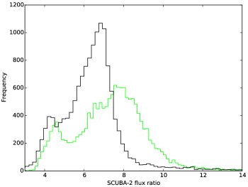
Figure 4: The distribution of 450 $\micron$/850 $\micron$ flux ratio for the original (black) and CO-subtracted (light grey line, green in the online version) Aquila reductions with additional 4^′ spatial filtering. KS-statistics reveal a 1.3% chance that the two data sets are drawn from the same distribution.

4 The free-free contribution to SCUBA-2 flux densities

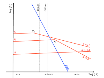
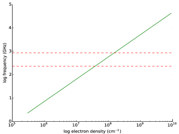
Figure 5: Left a schematic of the SED shape for three hypothetical scenarios of free-free emission. Case a) an UCH ii with $\alpha_{\mathrm{ff}}$ = 0.6 has a turnover that occurs short-ward of the submillimetre regime, and as a result has a majority contributions to the 850 $\micron$ band and a significant contribution to the 450 $\micron$ band. Case b) a YSO emits free-free emission, $\alpha_{\mathrm{ff}}$ = 1.0, from a collimated jet. However the spectrum turns over to the optically thin regime long ward of submillimetre wavelengths, and consequently free-free emission contributes roughly equally to both SCUBA-2 bands. Case c) an H ii region has free-free emission from diffuse gas of $\alpha_{\mathrm{ff}}$ = -0.1 that outshines that from compact objects at long wavelengths. However, the flat spectrum means that at submillimetre wavelengths the emission is all but negligible. Right free-free turnover as a function of launching electron density (as described by Olnon 1975 in Equation 1). Dashed lines indicate the submillimetre regime (1.3 mm to 350 $\micron$).

We examine now the arguments for thermal Bremsstrahlung, or free-free, contributions to the SCUBA-2 data. We address questions regarding the source, strength, spectral index, and frequency of the turnover (from partially optically thick to optically thin) of free-free emission. We examine the various sources of free-free emission in the W40 complex and assess the magnitude of the free-free contributions to both SCUBA-2 bands.

Free-free emission is typically observed from large-scale (1 pc), optically thin, diffuse H ii regions with an approximately flat (-0.1) spectral index, $\alpha_{\mathrm{ff}}$ (Oster, 1961; Mezger & Henderson, 1967). Free-free emission is also detected on smaller scales (Panagia & Felli, 1975) comparable to a protostellar core (0.05 pc, Rygl et al. 2013). On these smaller scales, free-free emission is produced by an ionised stellar wind (Wright & Barlow, 1975; Harvey et al., 1979) with an observed spectral index of $\alpha_{\mathrm{ff}}$ = 0.6 found by Harvey et al. (1979), Kurtz et al. (1994), and Sandell et al. (2011) where emission is considered partially optically thick. Where the wind is collimated and accelerating, as in bipolar jets, the spectral index increases to $\alpha_{\mathrm{ff}}\simeq$ 1.0 (Reynolds, 1986), as for example in AB Aur (Robitaille & Whitney, 2014) and MWC 297 (Rumble et al., 2015). In addition, non-thermal processes, such as gyrosynchrotron emission, have been known to lead to a negative spectral index (Hughes 1991, Hughes et al. 1995 and Garay et al. 1996).

4.1 Free-free emission in ultra compact H II regions

At small scales, free-free spectral indices are steep at low frequencies until the emission undergoes a turnover, $\nu_{c}$, as it transitions from being partially optically thick to optically thin. Figure 5 shows a schematic of the frequency behaviours of free-free emission, including this turnover. If the turnover occurs short-ward of submillimetre wavelengths, it is possible that free-free emission may contribute to the observed SCUBA-2 fluxes.

For a wind, the frequency of the free-free turnover is defined as a function of electron density, $n_{e}(r)$ = $n_{0}$ where $r$ $\leq$ $R$ and $n_{e}(r)$ = $n_{\mathrm{0}}(r/R)^{-2}$ where $r$ $\geq$ $R$, by Olnon (1975) as

$$\log_{10}\nu_{c}=-0.516+\frac{1}{2.1}\log_{10}\left(\frac{8}{3}Rn_{0}^{2}T_{e}^{-1.35}\right),$$ (1)

where $R$ is the launching radius of the wind (typically 10 AU) and $T_{e}$ is the electron temperature (typically 10⁴ K). Figure 5 (right) shows how $\nu_{c}$ is related to $N_{e,0}$. A minimum value of $N_{e,0}$ $\sim$ 2$\times$10⁸ cm^-3 is required for a turnover that occurs at wavelengths long ward of the submillimeter regime (1.3 mm to 350 $\micron$).

The electron density is not easily determined directly from observations. We assume that $n_{\mathrm{0}}$ is proportional to stellar mass and by association varies with spectral class. Sandell et al. (2011) indicate that the free-free contribution to SCUBA-2 fluxes is significant for early B stars in their sample, but not for late B- and A-type stars. For early B-stars, a distinct point source is observed at submillimetre wavelengths. In the case of the B1.5Ve/4V (Drew et al., 1997) Herbig star MWC 297 with an $\alpha_{\mathrm{ff}}$ = 1.03$\pm$0.02 (Skinner et al., 1993; Sandell et al., 2011), it was found that free-free emission contributed comparatively more to the 850 $\micron$ band (82$\pm$4 %) than to the 450 $\micron$ band (73$\pm$5 %) resulting in excessively low ratios (Rumble et al., 2015) that were misinterpreted as very low $\beta$ and potential grain growth by Manoj et al. (2007).

MWC 297 is the lowest mass star in the Sandell et al. (2011) sample for which free-free radiation contributes at SCUBA-2 wavelengths and we therefore mark it as a limit of stellar type. We therefore assume that a free-free turnover can occur in the submillimetre regime only for spectral types earlier than B1.5Ve/4V. This gives an indication of whether the free-free emission from a massive star is likely to be optically thin or thick at submillimetre wavelengths.

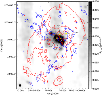
Figure 6: Archival VLA 21 cm NRAO VLA Sky Survey (Condon & Kaplan, 1998) continuum map of the W40 complex H ii region (45^′′ resolution greyscale). Red: Herschel 70 $\micron$ contours of the nebulosity Sh2-64 at 300, 1200, 4800, 12000 MJy/Sr. Blue: SCUBA-2 850 $\micron$ contours of the dust cloud at the 5 $\sigma$ level. Yellow stars indicate the locations of the OB stars, with the O9.5 star OS1 being the primary ionising object of the region. The white cross indicates the peak of the VLA 21 cm continuum emission.

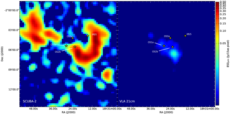
Figure 7: The free-free contribution from large-scale H ii gas, modelled using archival VLA 21 cm observations (Condon & Kaplan, 1998) assuming $\alpha_{\mathrm{ff}}$ = -0.1 (right), compared to SCUBA-2 dust emission at 850 $\micron$ (left). Maps have common 15^′′ pixels and 45^′′ resolution. Markers indicate the locations of the OB stars.

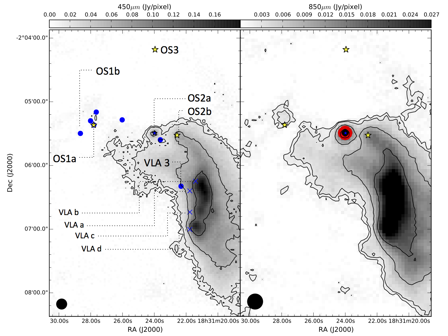
Figure 8: The free-free contribution of the compact radio source OS2a (marked as a blue star) at 450 $\micron$ (left) and 850 $\micron$ (right), modelled as point sources with fluxes extrapolated from the Rodriguez et al. (2010) 3.6 cm fluxes and assuming an $\alpha_{\mathrm{ff}}$ = 1.0. Yellow stars indicate the locations of the OB stars, blue filled circles the location of all the Rodriguez et al. (2010) and Ortiz-Le$\mathrm{\acute{o}}$n et al. (2015) compact radio source matches. Blue crosses mark the location of four peaks identified separately in the AUI/NRAO 3.6 cm map (450 $\micron$ only). Black contours trace SCUBA-2 data at 3$\sigma$, 5 $\sigma$, 15 $\sigma$ and 30$\sigma$. Red and black filled contours trace the optically thick free-free contribution at 3$\sigma$ and 5 $\sigma$ (see Table 3).

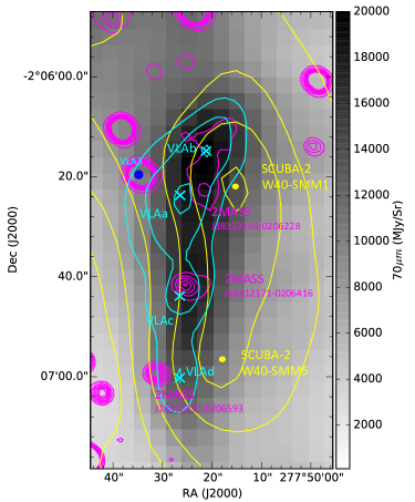
Figure 9: Archival Herschel 70 $\micron$ data for W40-SMM1 and 5. Magenta contours (560, 570, 580, 590, 600, 610, 620 mag.) show several 2MASS point sources embedded within the eastern Dust Arc which is shown in the yellow SCUBA-2 850 $\micron$ 5, 10, 20, 40, 60, 80$\sigma$ contours with circle markers at the peaks of the W40-SMM1 and 5 clumps (see Section 6). Cyan crosses show the four peaks in Archival AUI/NRAO 3.6 cm map (contours at 0.01, 0.016 and 0.021 Jy/beam). The Rodriguez et al. (2010) YSO ‘VLA3’ is also shown.

4.2 Free-free emission in the W40 complex

Free-free emission in the W40 complex comes from a large-scale H ii region associated with the nebulosity Sh2-64 (Condon & Kaplan, 1998), observed in archival VLA 21 cm continuum data presented in Figure 6. Vallee & MacLeod (1991) initially measured the size the H ii region as 6^′ by 3^′ with a 1.7^′ diameter incomplete shell. Pirogov et al. (2013) suggest a secondary H ii region powered by the B star IRS 5. However, we find no evidence for this in the 21 cm emission (Figure 6).

Table 3 lists several small-scale UCH ii regions associated with bright NIR objects in the W40 complex. Rodríguez et al. (2010) resolve 15 compact radio sources in 3.6 cm emission (at 0.26^′′ resolution) consistent with 2MASS sources and, by monitoring time-variability, are able to classify eight variable YSOs and seven non-variable UCH ii candidate regions. Ortiz-León et al. (2015) expand this survey and observe the same region at 4 cm and 6.7 cm, detecting 41 radio objects, 15 of which are confirmed as YSOs and are presented in Figure 8. Both Rodríguez et al. (2010) and Ortiz-León et al. (2015) also identify non-compact radio sources without IR counterparts and these are interpreted as shock fronts from thermal jets that are likely formed by the local Herbig AeBe stars OS1b and OS2a/b.

4.3 Contribution results

Building on the method outlined in Rumble et al. (2015), we model small- and large-scale free-free emission (separately). The contribution to SCUBA-2 maps is based either on a directly measured or an indirectly assumed value of $\alpha_{\mathrm{ff}}$.

For large-scale H ii emission, we extrapolate the archival VLA 21 cm data presented in Figure 6 up to SCUBA-2 wavelengths of 450 $\micron$ and 850 $\micron$, assuming a spectral index of $\alpha_{\mathrm{ff}}$ = -0.1 as concluded by Rodney & Reipurth (2008). The findback tool (see Appendix B) is used to remove structures larger than 5^′ (mimicking the SCUBA-2 data reduction process). Figure 7 shows how the SCUBA-2 data are subsequently aligned and convolved to the larger resolution of the VLA 21 cm data so the two data sets are comparable. The overall contribution of the large-scale H ii region to SCUBA-2 bands is very limited, at its peak contributing 5% at 850 $\micron$ and 0.5% at 450 $\micron$.

Ortiz-León et al. (2015) calculate the free-free spectral index for the 14 YSOs, marked in Figure 8, that are detected in both their 4 cm observations and the Rodríguez et al. (2010) 3.6 cm observations. The majority of YSOs have less than -0.1 $\alpha_{\mathrm{ff}}$ indicating non-thermal gyrosynchrotron emission that will not be bright at SCUBA-2 wavelengths and does not require further consideration. The OS1a cluster, OS2a, b and VLA-3 (J18312232-0206196) are all consistent with SCUBA-2 emission, as shown in Figure 8, and are considered for free-free contamination. These objects are summarised in Table 3.

OS1 is a dense stellar cluster that includes the primary ionising object, OS1a(South), that is driving the H ii region. Ortiz-León et al. (2015) calculate an $\alpha_{\mathrm{ff}}$ of -0.3$\pm$0.2 for this object which is consistent with an optically thin H ii region. The brightest radio source in the OS1 cluster is VLA-14 at 5.78 mJy at 3.6 cm (Table 3). It also has the most positive spectral index of $\alpha_{\mathrm{ff}}$ = 0.0$\pm$0.1. This corresponds to a peak 850 $\micron$ flux of 0.17 mJy, a value that falls well below the 1$\sigma$ noise level of that SCUBA-2 band. We therefore conclude that there is no evidence that free-free emission from the OS1a cluster is contributing to the faint 850 $\micron$ emission detected by SCUBA-2 (OS1a is not detected at 450 $\micron$).

Rodríguez et al. (2010) and Ortiz-León et al. (2015) calculate that VLA-3 has the most positive spectral index with $\alpha_{\mathrm{ff}}$ of 1.1$\pm$0.2. This index is consistent with a collimated jet source. Zhu et al. (2006) and Shimoikura et al. (2015) studied the ¹³CO 2–1, ¹²CO 1–0 and 3–2 line emission in this region and observed profiles symptomatic of outflows. However, we observe that the ¹²CO 3–2 line in this region is highly extincted due to emission becoming optically thick at high densities, making reliable analysis of these features impractical. Figure 8 shows that VLA-3 is heavily embedded within the Dust Arc; however, it is not associated with a strong point source in either SCUBA-2 bands in the same way that OS2a is. From this we conclude that free-free emission from YSO VLA-3 has turned over to optically thin at wavelengths longer than the submillimeter regime and does not provide a significant contribution to the SCUBA-2 bands.

OS2a is a Herbig AeBe star that is detected as a strong point source by SCUBA-2 at both 450 $\micron$ and 850 $\micron$ (Figure 8). Rodríguez et al. (2010) detect OS2a at 3.6 cm, finding it to be variable and having evidence for jets through outflow knots. By contrast Ortiz-León et al. (2015) detect emission at the location of OS2a, but do not report it as its SNR falls below their detection criteria (Ortiz-Leon. priv. comm.). Such behaviour is consistent with a variable object, and therefore it is not possible calculate a reliable $\alpha_{\mathrm{ff}}$.

In order to make an estimate of the upper limit of the free-free contribution of OS2a, we model OS2a as a point source and extrapolate the Rodríguez et al. (2010) 3.6 cm flux up to 450 and 850 $\micron$ based on an $\alpha_{\mathrm{ff}}$ of 1.0, consistent with indirect observations of local jet emission by Rodríguez et al. (2010). We make the optimistic assumption that OS2a is optically thick at SCUBA-2 wavelengths on the basis of the bright point source at that location that is observed at 450 and 850 $\micron$ (Figure 8). The fluxes are subsequently convolved by the JCMT beam using its primary and secondary components for comparison with the SCUBA-2 data and presented in Table 4. Using this method we calculate that the free-free contribution for OS2a is at most 9% at 450 $\micron$ and 12% at 850 $\micron$.

No radio or submillimeter point source has been observed at the location of OS2b, as shown in Figure 8. We therefore assume that any free-free radio emission must be faint and optically thin at SCUBA-2 wavelengths. This is consistent with its classification as a weak UV-photon-emitting B4 star (Shuping et al., 2012).

Table 3: Summary of bright radio objects in the W40 complex and evidence for variability, jet emission and free-free opacity at SCUBA-2 wavelengths, from which a value of $\alpha_{\mathrm{ff}}$ can be estimated (if not previously calculated).

Source	2MASS ID	VLA IDa	Type b	Time a	Jeta?	SCUBA-2	Optically	Spectral index	Distanceb
				variable?		source?	thick?	$\alpha_{\mathrm{ff}}$	(pc)
OS 1a (North)	J18312782-0205228	15	Herbig AeBe	N	N	Y	Y	-0.3$\pm$0.2c	536${}^{+42}_{-95}$
OS 1a (South)	J18312782-0205228	-	O9.5	-	N	Y	-	-	536${}^{+42}_{-95}$
OS 1b	J18312866-0205297	18	Class II	N	Y	N	N	-0.8$\pm$0.5c	-
OS 1c	J18312601-0205169	8	Class II	Y	N	N	N	-0.6$\pm$0.2c	-
OS1d	J18312766-0205097	13	Class II	Y	N	Y	N	0.1$\pm$0.2c	-
OS 2a	J18312397-0205295	7	Herbig AeBe	Y	Y	Y	Y	1.0	-
OS 2b	J18312257-0205315	-	B4	Y	Y	N	N	-0.1	455${}^{+71}_{-59}$
OS 3	J18312395-0204107	-	B3*(binary)	-	-	N	-	-	454${}^{+87}_{-48}$
IRS 5	J18311482-0203497	1	B1	-	-	N	N	0.3$\pm$0.2c	469${}^{+217}_{-129}$
-	J18312232-0206196	3	Class II	N	Y	N	N	1.1$\pm$0.2c	-
-	-	14	-	N	N	N	N	0.0$\pm$0.1c	-

^a Radio source ID and characterisation based on the findings of Rodríguez et al. (2010).
^b Spectral classifications and distances calculated from Spectral Energy Distributions in Shuping et al. (2012).
^c Free-free spectral index calculated by Ortiz-León et al. (2015).

Table 4: Summary of significant free-free contributions to SCUBA-2 wavelengths from bright objects in W40. The uncertainty on flux density at 450 $\micron$ is 0.017 Jy/pix and 850 $\micron$ is 0.0025 Jy/pix.

	3.6 cm (Jy)	450 $\micron$ (Jy)				850 $\micron$ (Jy)
Object	VLAa	SCUBA-2	Free-free	Dust	%	SCUBA-2	Free-free	Dust	%	$\alpha_{\mathrm{ff}}$
OS2a	0.00240	1.83	0.16	1.67	9	0.558	0.069	0.489	12	1.0

^a VLA 3.6 cm compact object fluxes (Rodríguez et al., 2010).

4.4 Additional free-free sources

Observations by Rodríguez et al. (2010) did not cover the four brightest peaks in the AUI/NRAO 3.6 cm data that lie to the west of VLA-3, referred to here as VLAa, b, c, and d (Figure 8 and 9). These objects are orders of magnitude brighter than the Rodríguez et al. (2010) sources and appear in close proximity to the peak 850 $\micron$ emission and three 2MASS sources. Each 2MASS source is deeply reddened, consistent with an embedded YSO, suggesting that these objects could be young protostars. Examining the 70 $\micron$ data (Figure 9), where the blackbody spectrum of a protostar is at its peak, FIR emission is brightest around the location of J18312144-0206228 and J18312171-0206416. Their respective alignment with VLAa /VLAc could be considered as an indicator of an UCH ii region around a massive protostar. This idea is consistent with the findings of Pirogov et al. (2013) who observe CS 2 –1 line emission and find evidence of infalling material linked to high-mass star-formation in the eastern Dust Arc.

Alternatively, we could be observing free-free emission from the shock/ionisation front from where the OS1a H ii region is interacting with the eastern Dust Arc, as proposed by Vallee & MacLeod (1991). Using flux and distance in Kurtz et al. (1994)’s Equation 4, we calculate that a Lyman photon density of 4.0$\times$10⁴⁶ s^-1 is required to produce a total flux density of 0.167 Jy for all four unidentified VLA sources at 3.6 cm. We compare this value to the Lyman photon density produced by OS1a, a 09.5V star, which is the primary ionising source of the H ii region. We assume a minimum distance between OS1a and the filament of 3^′, consistent with Vallee & MacLeod (1991), and calculate that the proposed ionisation front across the eastern Dust Arc would be exposed to, at most, 2.1% of Lyman photons produced by OS1a at this distance. This percentage corresponds to a Lyman photon density of 1.67$\times$10⁴⁶ s^-1, which is comparable to the flux observed given the approximate nature of this calculation.

Given the speculation about the nature of these sources, we cannot reliably estimate a value of $\alpha_{\mathrm{ff}}$ for these objects. However, we do not observe significant SCUBA-2 peaks at the positions of these objects. We therefore conclude that any free-free emission observed here at 3.6 cm is optically thin at SCUBA-2 wavelengths and therefore regardless of their nature they produce no significant free-free contributions.

5 Temperature mapping

In this section we outline how the dust temperature is calculated from the ratio of SCUBA-2 fluxes at a common resolution, obtained using a convolution kernel, and how this method compares to our previous work with the dual-beam cross-convolution method described in Rumble et al. (2015). We present the temperature maps for the W40 complex and outline some of their notable features.

By taking the ratio of SCUBA-2 fluxes at 450 and 850 $\micron$, the spectral index of the dust, $\alpha$, can be calculated as a power law of frequency ratio,

$$\frac{S_{\mathrm{450}}}{S_{\mathrm{850}}}=\left(\frac{\nu_{850}}{\nu_{450}}\right)^{\alpha},$$ (2)

where $\alpha$ can be approximated to 2 + $\beta$ (assuming the Rayleigh-Jeans limit). By assuming a full, opacity-modified Planck function, it is possible to show that $\alpha$ is derived from $\beta$ and the dust temperature, $T_{\mathrm{d}}$. As a result, Equation 2 can be expanded into

$$\frac{S_{\mathrm{450}}}{S_{\mathrm{850}}}=\left(\frac{850}{450}\right)^{3+\beta}\left(\frac{\exp(hc/\lambda_{\mathrm{850}}k_{\mathrm{b}}T_{\mathrm{d}})-1}{\exp(hc/\lambda_{\mathrm{450}}k_{\mathrm{b}}T_{\mathrm{d}})-1}\right)$$ (3)

to include both of these parameters (Reid & Wilson, 2005). By assuming a constant $\beta$ across a specific region, maps of temperature are produced for the W40 complex by convolving the 450 $\micron$ map down to the resolution of the 850 $\micron$ map using an analytical beam model convolution kernel (Aniano et al. 2011, Pattle et al. 2015, see Section 5.1 and Appendix A for details).

The relationship between wavelength and dust opacity is modelled as a power-law for a specific dust opacity spectral index in the submillimetre regime,

$$\kappa_{\lambda}=0.012\times\left(\frac{\lambda}{850\mu\mathrm{m}}\right)^{-\beta}\mathrm{cm^{2}/g},$$ (4)

which is consistent with the popular OH5 model (Ossenkopf & Henning, 1994) of opacities in dense ISM, for a specific gas-to-dust ratio of 161 and $\beta$ = 1.8 over a wavelength range of 30 $\micron$–1.3 mm (Hatchell et al., 2005). This value is consistent with Planck observations (Juvela et al., 2015) and that used in other GBS papers (Salji et al. 2015, Rumble et al. 2015 and Pattle et al. 2015), but less than the Planck Collaboration et al. (2011) who find a mean value of $\beta$ = 2.1 in cold clumps.

The majority of the structure observed in the W40 complex is typical of the ISM and protostellar envelopes and our use of $\beta$ = 1.8 (Hatchell et al., 2013) reflects a standard approach, though $\beta$ has been found up to 2.7 in extended, filamentary regions (Planck Collaboration et al. 2011, Chen et al. submitted) and around 1.0 in discs (Beckwith et al., 1990; Sadavoy et al., 2013; Buckle et al., 2015).

A popular alternative to the SCUBA-2 flux ratio method discussed above is spectral energy distribution (SED) fitting, a method that has been widely used to derive both dust temperatures and $\beta$ from Herschel (Griffin et al., 2010) SPIRE and PACS bands (Shetty et al. 2009, Bontemps et al. 2010 and Gordon et al. 2010). SED fitting can be limited by the emission model, the completeness of the spectrum, resolution and local fluctuations of $\beta$ (Könyves et al., 2010). A detailed comparison between the SCUBA-2 flux ratio method and SED fitting is given in Appendix D. A comparison with the temperatures calculated by Maury et al. (2011) and Könyves et al. (2015) using SED fitting is given in Section 6.

5.1 The convolution kernel

The JCMT has a complex beam shape and different resolution at each of the SCUBA-2 bands and a common map resolution is required before the flux ratio can be calculated. Achieving common resolution of maps by using a kernel, as opposed to the cross-convolution with JCMT primary and secondary beams (see Rumble et al. 2015), has the advantage of improved resolution flux ratio maps. The kernel method results in a temperature map with a resolution of 14.8^′′, approximately equal to the 850 $\micron$ map, whereas the resolution of the dual-beam method is 19.9^′′.

We apply the kernel convolution algorithm from Aniano et al. (2011) using the Pattle et al. (2015) adaptation to SCUBA-2 images. Details of the method are summarised in Appendix B and those authors’ papers. Having achieved common resolution, ratio and temperature maps are produced following the method of Rumble et al. (2015). Details of the propagation of errors through the convolution kernel are also given Appendix B.

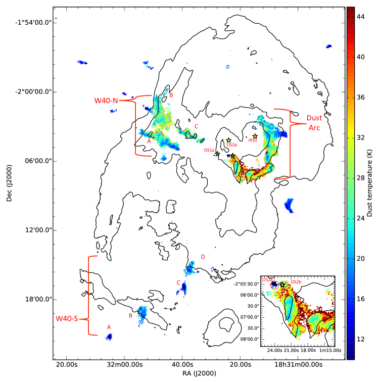
Figure 10: Temperature map of the W40 complex with Herschel 70 $\micron$ contours at 300, 1200, 4800 and 12000 MJy/Sr. Note that 850 $\micron$ flux has been decontaminated for CO in all areas except W40-S. Temperatures are given at positions where the 850 $\micron$ flux is at least five times the noise level and the fractional error on the temperature is less than 0.34. The insert shows a zoom in on the Eastern Dust Arc and the high mass stars OS2a/b.

5.2 Temperature and spectral index results

Table 5: A sample of submillimetre clumps and their respective SCUBA-2 and Herschel fluxes. The full table is available online.

Indexa	IAU object namea	70 $\micron$ intensityb	450 $\micron$ fluxc	850 $\micron$ fluxc	21 cm intensityd	Clump area
		(MJy/Sr)	(Jy)	(Jy)	(Jy/pix)	(Pixels)
W40-SMM1	JCMTLSG J1831210-0206203	8304	93.50	10.44	0.124	759
W40-SMM2	JCMTLSG J1831102-0204413	3834	56.38	6.77	0.006	422
W40-SMM3	JCMTLSG J1831104-0203503	3622	71.64	9.26	0.005	807
W40-SMM4	JCMTLSG J1831096-0206263	1982	26.72	3.06	0.011	189
W40-SMM5	JCMTLSG J1831212-0206563	5007	41.98	4.73	0.091	350
W40-SMM6	JCMTLSG J1831106-0205413	2322	54.28	6.54	0.008	438
W40-SMM7	JCMTLSG J1831168-0207053	4854	62.94	6.87	0.013	514
W40-SMM8	JCMTLSG J1831468-0204263	2185	46.21	5.96	0.003	405
W40-SMM9	JCMTLSG J1831388-0203353	3533	32.30	3.77	0.015	313
W40-SMM10	JCMTLSG J1831038-0209503	344	24.63	3.57	0.004	389

^aPosition of the highest value pixel in each clump (at 850 $\micron$).
^bMean Herschel 70 $\micron$ intensity.
^cIntegrated SCUBA-2 fluxes over the clump properties. The uncertainty at 450 $\micron$ is 0.017 Jy/pix and at 850 $\micron$ is 0.0025 Jy/pix. There is an additional systematic error in calibration of 10.6 % and 3.4 % at 450 $\micron$ and 850 $\micron$, respectively.
^dMean VLA 21 cm intensity at 15^′′ pixels.

The SCUBA-2 temperature and flux spectral index $\alpha$ of the W40 complex, calculated from post-CO, post-free-free reduced maps are presented in Figures 10 and 11 respectively. The range of dust temperatures (9 to 63 K) in the W40 complex is presented in Figure 12 and is comparable to those calculated from SCUBA-2 data in NGC1333 by Hatchell et al. (2013) and in Serpens MWC 297 by Rumble et al. (2015).

We break the complex into major star-forming clouds. The Dust Arc, W40-N, and W40-S have mean temperatures of 29, 25 and 18 K, respectively. Figure 12 presents the distribution of temperatures in these clouds. The highest temperature pixels (in excess of 50 K) are found in the eastern Dust Arc whilst the lowest temperature pixels (9 K) are associated with OS2a.

A map of the SCUBA-2 flux spectral index (Figure 11) is a more objective summary of the submillimetre SED. We find that $\alpha$ values are fairly constant across the filaments of the W40 complex with a mean $\alpha$ = 3.1$\pm$0.2, as expected for the ISM with $\beta$ = 1.8 and temperature approximately 20 K. However, the value of $\alpha$ associated with OS2a (marked in Figure 10) is notably lower with a minimum value of $\alpha$ = 1.6$\pm$0.1.

A low $\alpha$ has previously been explained by very low $\beta$, associated with grain growth (Manoj et al., 2007), or low temperatures. Rumble et al. (2015) demonstrated that lower spectral indices can also be caused by free-free emission contributing to SCUBA-2 detections, but in this case the free-free emission does not have a significant impact on $\alpha$. SCUBA-2 dust temperatures towards OS2a are some of the lowest in the whole region with values less than 9 K (see Figure 10 insert). Given a $\beta$=1.0, typical for circumstellar disks, $\alpha$ = 1.6 would require an unphysical temperature of less than 2 K. Alternatively, an exceptionally low $\beta$ approaching zero would still require an excessively low temperature of less than 7 K, comparable to the SCUBA-2 dust temperature of 9 K (see Figure 10 insert) observed at $\beta$=1.8. It is therefore unlikely that $\beta$ alone can explain these results.

OS2a was detected by the VLA in Rodríguez et al. (2010) in the autumn 2004 and noted as a variable radio source. Subsequent observations by Ortiz-León et al. (2015) in summer 2011 failed to make a significant detection of OS2a, confirming the object as highly variable. The transient nature of OS2a could offer an alternative explanation for the exceptionally low dust spectral index observed by SCUBA-2 in the summer 2012. We note that Maury et al. (2011) calculates a dust temperature of 40$\pm$8 K for OS2a from the 2 $\micron$ - 1.2 mm SED which incorporates observations from 2007 and 2009. Further work is required to fully address the nature of this source.

6 The SCUBA-2 clump catalogue

To analyse individual star-forming regions, we use the Starlink fellwalker algorithm (Berry, 2015) to identify clumps in the SCUBA-2 850 $\micron$, CO subtracted, 4^′ filtered, free-free subtracted map. Details of fellwalker and the parameters used to refine clump selection are given in Appendix E. We identify 82 clumps in the W40 complex and their fluxes at 850 $\micron$, as well as 70 $\micron$, 450 $\micron$ and 21 cm from Herschel, SCUBA-2 and Archival VLA maps, respectively, are presented in Table 5. Clump positions in the W40 complex are presented in Figure 13. The outer boundary of the clumps approximately corresponds to the 5 $\sigma$ contour in Figure 3 (upper panel).

6.1 Clump temperatures

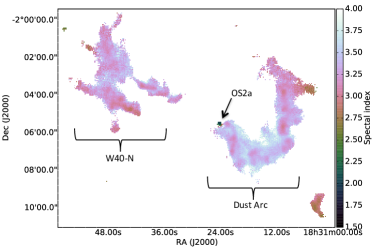
Figure 11: SCUBA-2 spectral index $\alpha$ of W40-N and the Dust Arc. The spectral index for W40-S is not shown but is similar in value to W40-N.

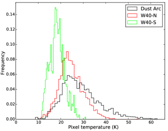
Figure 12: The normalised distribution of pixel temperatures across the W40 complex clouds: Dust Arc (black, warmest), W40-N (red) and W40-S (green, coolest).

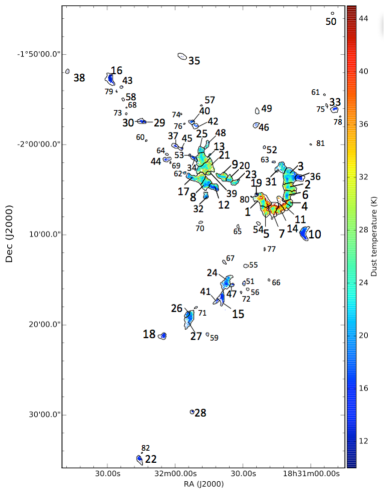
Figure 13: Temperature map of the W40 complex with clumps identified in the SCUBA-2 CO subtracted, 4^′ filtered, and free-free subtracted 850 $\micron$ data using the Starlink clump-finding algorithm fellwalker plotted as contours. Clumps are indexed in order of highest to lowest flux density, matching the order presented in Tables 5 and 6.

The unweighted mean value of temperature across all of the pixels in a clump in the W40 complex is calculated and presented in Table 6. There are no temperature data for 21 clumps as they are not detected at 450 $\micron$ above the 5 $\sigma$ noise level (0.0035 Jy per pixel). For these cases we assign a temperature of 15$\pm$2 K, consistent with Rumble et al. (2015). Where temperature data only partially cover the 850 $\micron$ clump, we assume the vacant pixels have a temperature equal to the mean of the occupied pixels.

Partial coverage tends to occur at the edges of clumps as a result of lower signal-to-noise at 450 µm flux, relative to 850 µm flux. Setting missing pixels to the clump average could introduce a temperature bias if clump edges are systematically warmer (or colder) than the clump centres. This was tested by replacing vacant pixels with the average of the top 20% of pixels values in each clump, rather than the average of all the pixels, given the assumption that the edges of the clumps were warmer than their centres. We found the mean clump temperature increased by at most 2.2K (averaged over all clumps). From observation, only a few clumps have systematically warmer edges, whereas the majority of clumps have warm pixels randomly distributed within them. We therefore treat this value as an upper limit on any bias.

Where a clump carries only a small number of temperature pixels, the recorded clump temperature is unlikely to be representative of the whole clump. We find that 20 % of clumps are missing more than 75 % of the total potential temperature pixels with the most prominent of this set being W40-SMM 35. The following discussion concerns only clumps with complete or partial temperature data.

Figure 14 (lower left) shows the distribution of derived temperatures. The W40 complex has a mean clump temperature of 20$\pm$3 K with a mean percentage error across all clumps of 16% due to calibration uncertainty. The mean temperature of the peripheral clumps (i.e. those not attributed to W40-N, W40-S or the Dust Arc) is 15$\pm$2 K, equal to that found in the Serpens MWC 297 region (Rumble et al., 2015) and the assumptions used by Johnstone et al. (2000), Kirk et al. (2006) and Sadavoy et al. (2010) for isolated clumps. These findings are consistent with those of Foster et al. (2009) who found that isolated clumps in Perseus were systematically cooler than the those in clusters.

We compare our clump temperatures to those calculated by Maury et al. (2011) and Könyves et al. (2015) using SED fitting between, 2 $\micron$ and 1.2 mm, for sources extracted using the getsources algorithm. Our mean temperature of the 19 sources common to all three catalogues is 19.8$\pm$2.8 K. This is comparable to the Maury et al. (2011) value of 18.5$\pm$0.4 K, but higher than the Könyves et al. (2015) value of 14.1$\pm$1.3 K. Whilst all three methods calculate similar minimum source temperatures (10-12 K), our method calculates the highest maximum source temperatures (33.6 K, compared to 27.0 K and 20.6 K in Maury et al. 2011 and Könyves et al. 2015, respectively). This is because the warmest dust lies in the low column density edges of filaments (see Figure 10) where it is likely to be omitted by the getsources algorithm, which is optimised to find centrally condensed cores.

Figure 15 shows clump temperature as a function of projected distance from OS1a. The clumps at distances greater than 1.2 pc (marked) have near-constant temperatures (on average 16$\pm$3 K), again consistent with those of isolated clumps (Johnstone et al. 2000, Kirk et al. 2006 and Rumble et al. 2015). At distances of less than 1.2 pc there is a strong negative correlation between temperature and projected distance to OS1a. The lower panel in Figure 15 shows how clump temperature does not increase significantly given the presence of a protostar with all protostellar clumps having the same mean temperature (as a function of distance) as the starless clumps, within the calculated uncertainties. This suggests that internal heating from a protostar is not significant enough to raise the temperatures of clumps in the W40 complex. However, use of a constant $\beta$ = 1.8, consistent with the ISM, may mask heating in protostars where low values of $\beta$ have been observed (Chen et. al, submitted).

VLA 21 cm continuum data trace free-free emission from the super-heated H ii region. Figures 6 and 7 show the extent of the H ii region and where it coincides with several of the SCUBA-2 clumps in the Dust Arc and W40-N. The size of the H ii region corresponds to a 0.17  pc radius, but Figure 15 shows temperatures increasing inversely with radius from OS1a out to 1.2 pc (8.25^′). Figure 16 shows none of the clumps within the H ii region has a temperature of less than 21 K (ignoring W40-SMM 19) and the mean clump temperature of 29 K is almost twice the temperature of an isolated clump. Our conclusions support the Matzner (2002) model where radiative feedback from the OB association (including ionising and non-ionising photons) is the dominant external mechanism for heating clumps.

Table 6: The properties of a sample of submillimetre clumps in the W40 complex. The full table is available online.

Index	S850a	Massb	Tempc.	Column densityd	YSO densitye	Protostarse	MJf	M/MJ	Distanceg
	(Jy/pixel)	(M⊙)	(K)	(H2 cm-2)	(YSO pc-2)	(per clump)	(M⊙)		(pc)
W40-SMM1	0.046	12.5$\pm$2.6	33.6$\pm$5.7	75$\pm$16 $\times$1021	147	4	20.6$\pm$3.5	0.6$\pm$0.2	0.3
W40-SMM2	0.041	9.7$\pm$1.7	28.1$\pm$3.7	69$\pm$12 $\times$1021	17	0	12.9$\pm$1.7	0.8$\pm$0.2	0.6
W40-SMM3	0.040	16.6$\pm$3.3	23.0$\pm$3.2	83$\pm$17 $\times$1021	22	1	14.6$\pm$2.0	1.1$\pm$0.3	0.7
W40-SMM4	0.040	4.0$\pm$0.6	30.2$\pm$3.9	62$\pm$10 $\times$1021	26	1	9.2$\pm$1.2	0.4$\pm$0.1	0.7
W40-SMM5	0.037	5.6$\pm$1.1	33.1$\pm$5.5	57$\pm$12 $\times$1021	86	1	13.8$\pm$2.3	0.4$\pm$0.1	0.3
W40-SMM6	0.036	9.9$\pm$1.7	27.8$\pm$3.7	73$\pm$12 $\times$1021	21	1	12.9$\pm$1.7	0.8$\pm$0.2	0.6
W40-SMM7	0.030	7.3$\pm$1.5	35.8$\pm$6.0	44$\pm$9 $\times$1021	47	0	18.1$\pm$3.0	0.4$\pm$0.1	0.5
W40-SMM8	0.030	10.8$\pm$1.7	23.8$\pm$2.8	60$\pm$10 $\times$1021	25	1	10.6$\pm$1.3	1.0$\pm$0.2	0.7
W40-SMM9	0.029	6.0$\pm$1.2	26.3$\pm$4.2	48$\pm$10 $\times$1021	56	0	10.4$\pm$1.6	0.6$\pm$0.2	0.5
W40-SMM10	0.027	10.5$\pm$1.8	16.5$\pm$1.6	80$\pm$14 $\times$1021	36	2	7.3$\pm$0.7	1.5$\pm$0.3	1.1

^aPeak SCUBA-2 850 $\micron$ flux of each clump. The 850 $\micron$ uncertainty is 0.0025 Jy/pix. There is a systematic error in calibration of 3.4 %.
^bAs calculated with Equation 5. These results do not include the systematic error in distance (10 %) or opacity (up to a factor of two).
^cMean temperature as calculated from the temperature maps. Uncertainty is the mean pixel standard deviation, as propagated through the method. Where no temperature data are available an arbitrary value of 15$\pm$2 K is assigned that is consistent with previous authors (Johnstone et al. 2000, Kirk et al.,2006, Rumble et al.2015).
^dPeak column density of the clump. These results do not include the systematic error in distance or opacity.
^eCalculated from the composite YSO catalogue outlined in Section 2.3.
^fAs calculated with Equation 7. These results do not include the systematic error in distance.
^gProjected distance between clump and OS1a, the primary ionising star in the W40 complex OB association.

6.2 Clump column densities and masses

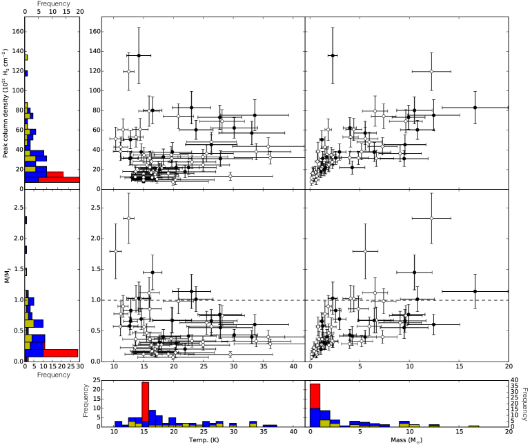
Figure 14: Properties of clumps within the W40 complex. Histograms show the distribution of mass, temperature, $\mathrm{M/M_{J}}$ and peak column density. Total height of each bar represents the total number of clumps in each bin whereas each colour represents a specific subset: blue for clumps that have measured temperature, yellow for clumps with measured temperatures that contain at least one YSO, and red for clumps with no temperature data, for which the value 15$\pm$2 K is assumed. Scatter plots show any existing correlation between clump properties: top left shows column density as a function of temperature, top right shows column density as a function of mass, bottom left shows Jeans stability, M₈₅₀/M_J, as a function of temperature and bottom right shows Jeans stability as a function of mass. Filled markers indicate protostellar clumps and hollow markers indicate starless clumps.

Masses of the clumps in the W40 complex are calculated by assuming a single temperature grey body spectrum (Hildebrand, 1983). We follow the standard method for calculating clump mass for a given distance, $d$, and dust opacity, $\kappa_{\mathrm{850}}$, (Johnstone et al. 2000; Kirk et al. 2006; Sadavoy et al. 2010; Enoch et al. 2011). Clump masses are calculated by summing the SCUBA-2 850 $\micron$ flux, per pixel $i$ (in Jy per pixel) using

$$M =0.39\sum_{i}S_{{\mathrm{850},i}}\left[\exp\left(\frac{17\,\mathrm{K}}{T_{\mathrm{d},i}}\right)-1\right]$$ (5)

$$\times\left(\frac{d}{250\,\mathrm{pc}}\right)^{2}\left(\frac{\kappa_{\mathrm{850}}}{0.012\,\mathrm{\hbox{cm}^{2}\hbox{g}^{-1}}}\right)^{-1}\,\mathrm{M_{\odot}}.$$

The dust opacity, $\kappa_{\mathrm{850}}$, is given in Equation 4 and we assume a distance $d=500\pm 50\hbox{ pc}$ following Mallick et al. (2013), as outlined in Section 1.

We can also incorporate temperature measurements alongside the SCUBA-2 850 $\micron$ fluxes (Equation 5) to calculate pixel column densities, N${}_{i,H_{2}}$, from pixel masses, M_i, using the pixel area, A_i, and the mean molecular mass per H₂, $\mu$=2.8 (Kauffmann et al., 2008),

$$N_{i,H_{2}}=\frac{M_{i}}{\mu_{H_{2}}m_{p}A_{i}}.$$ (6)

Peak column densities per clump are also presented in Table 6. Figure 17 presents a map of column density. Figure 14 (upper left) shows the distribution of peak column densities in the W40 complex as a function of temperature.

We find a minimum peak column density of 1.7$\times$10²² H₂ cm^-2 for clumps containing a protostar. Above this value there is no significant correlation between peak column density and temperature or protostellar occupancy. The upper right panel of Figure 14 shows how peak column density is tightly correlated with mass in the clumps. Above 3 M_⊙, the correlation is looser with several examples of clumps of similar column density having masses varying between 3 and 12 M_⊙.

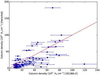
Figure 18: The peak column density of SCUBA-2 clumps compared to Herschel sources, as published by K$\mathrm{\ddot{o}}$nyves et al. (2015). A parity line is marked in red. Clump pairs are matched within a separation of 15^′′.

The peak column density of Herschel sources, detected by Könyves et al. (2015), are compared to 69 matching (within 15^′′, one JCMT beam width at 850 $\micron$) SCUBA-2 clumps as this value is independent of clump size. Figure 18 shows that the two sets are loosely correlated. The mean peak column density of the SCUBA-2 clumps (3.2$\pm$0.7$\times$10²² H₂ cm^-2) is comparable to that of the Herschel sources (2.6$\times$10²² H₂ cm^-2). It is notable that the majority of objects have a lower peak column density recorded by Herschel than by SCUBA-2. This can be explained by the SED fitting method used by Könyves et al. (2015) which can be biased towards higher temperature clouds, and has a lower resolution of 36.6^′′ (consistent with the Herschel 500 $\micron$ beam size).

We calculate a lower limit on the average volume density along the line of sight for clumps from the ratio of peak column density and clump depth (assumed equal to the flux weighted clump diameter as calculated by fellwalker, which is equivalent to the clump FWHM, see Appendix E for more info).

From our sample of clumps, Table 7 lists 31 ‘dense cores’ with a volume density greater than 10⁵ cm^-3, along with any protostars within these clump and their respective Jeans stabilities (see section 6.3). At densities greater than 10^4.5 cm^-3 we can be confident the dust and gas temperatures are well coupled (Goldreich & Kwan 1974 and Goldsmith 2001). Dense cores account for approximately 63% of the mass observed by SCUBA-2 at 850 $\micron$. The Dust Arc has nine dense cores, W40-N has nine, W40-S has four, and there are 11 isolated dense cores. In total, 42% of the dense cores contain at least one protostar, confirming that a significant proportion of clumps in the W40 complex is likely to be undergoing star-formation.

6.3 Clump stability

Jeans stability (Jeans, 1902) of the clumps is measured by a critical ratio, above which self-gravity will overwhelm thermal support in an idealised cloud of gas, causing it to collapse and begin star-formation.The condition for collapse is defined as when the mass of a clump, M₈₅₀, is greater than its Jeans mass,

$$M_{\mathrm{J}}=1.9\left(\frac{\bar{T}_{\mathrm{g}}}{10\,\mathrm{K}}\right)\left(\frac{R_{\mathrm{c}}}{0.07\,\mathrm{pc}}\right)\,\mathrm{M}_{{{\sun}}},$$ (7)

where R_c is an effective radius produced by fellwalker from the clump area (in pixels) assuming spherical structure. This measure of R_c is typically twice the flux weighted clump radius and better represents the complete extent of the clump. The gas temperature $\bar{T_{g}}$ (assumed isothermal in the theory) is taken to equal the mean dust temperature of the clump. We note that the dust and gas may be poorly coupled for clumps not included in our dense cores list ($n>10^{5}\hbox{ H}_{2}\hbox{ cm}^{-3}$; see Table 7); if gas temperatures drop below the dust temperature (Tielens & Hollenbach, 1985), their Jeans stability may be overestimated. Additional forces such as magnetism and turbulence could provide additional support against gravitational collapse (as explained in, Sadavoy et al. 2010 and Mairs et al. 2014).

Due to the high optical depth of our ¹²CO 3-2 line data, it is not possible to use these data to calculate the turbulent support. Arzoumanian et al. (2011) calculate a sonic scale of 0.05–0.15 pc below which the sound speed is comparable to the velocity dispersion and turbulent pressure dominates over thermal pressure. This scale range includes 83% of all the clumps in the W40 complex so our working assumption (in the absence of direct measurements) is that the majority of the W40 complex is subsonic or transonic. This is supported by observations of starless cores in Ophiuchus, which is similarly located on the edge of an OB association; these cores are transonic or mildly supersonic (Pattle et al., 2015). Providing the W40 complex is similar, then clumps could be stable against gravitational collapse to a few times the Jeans mass. Magnetic support is poorly characterised and also left out of our stability analysis.

Jeans stability (M₈₅₀/M_J) values for each clump are presented in Table 6, Table 7 and Figure 14 (lower left). Out of 82 clumps in the W40 complex, we find that 10 are unstable with M₈₅₀/M${}_{\mathrm{J}}\geq$ 1. Given the likely variety in clump morphologies, only those with M₈₅₀/M${}_{\mathrm{J}}\geq$ 2 can be considered truly unstable (Bertoldi & McKee, 1992); the stability threshold is raised further if turbulent support is significant.

As with column density, we find M₈₅₀/M_J is tightly correlated with mass below 3 M_⊙ and more loosely correlated above 3 M_⊙. We can also determine that M₈₅₀/M_J is loosely negatively correlated with temperature; see bottom left panel of Figure 14. Below 24 K there is a mixture of stable and unstable clumps but above this temperature all clumps are stable.

W40-SMM 14 is an example of a clump with high M₈₅₀/M_J (0.3) and high temperature (36 K). Measuring the clump radius as 0.05 pc and flux as 3.96 Jy, we can estimate using Equations 5 and 7 that if this clump had a typical temperature of 15 K, it would have a mean M₈₅₀/M_J of 6.5. Whilst this number is only an estimate, it is over 20 times the measured value and therefore we are confident that the raised temperature of this clump is reducing M₈₅₀/M_J and potentially suppressing collapse. The two most unstable clumps are W40-SMM 16 (2.3$\pm$0.4) and 35 (1.8$\pm$0.4) which are cold, isolated clumps on the periphery of the W40 complex. W40-SMM 16 contains a protostar whereas 35 is currently starless.

The eastern Dust Arc is positioned on the edge of the H ii region. Raised temperatures mean that clumps here have a mean Jeans mass of 17 M_⊙ for clumps in the eastern Dust Arc, compared to 12 M_⊙ in the western Dust Arc, and 5 M_⊙ for the average clump in the W40 complex. Likewise the median M₈₅₀/M_J is 0.4 compared to 0.8 in the western Dust Arc which is considered outside of the H ii region and consequently has lower temperatures. Note that both filaments have similar mean clump masses of these regions (7 and 8 M$\odot$, respectively). Given its common CO gas velocity (Figure 3 upper) the Dust Arc, as a whole, is likely a continuous filament, and therefore we might expect its clumps to evolve at a similar rate due to similar initial conditions along the length of the filament. Significant differences in stabilities along the length of the filament as a result of heating by the OB association, however, hint that star-formation may take place there at different rates.

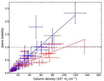
Figure 19: Jeans stability, M₈₅₀/M_J, as a function of column density. Exterior peripheral clumps (defined as having a mean Herschel 70 $\micron$ flux of less than 1000 MJy/Sr) are marked in blue, interior clumps within the nebulosity Sh2-64 are marked in red. The unweighted linear regression fit to each population is marked as a line of the same colour.

We further examine the impact of radiative heating by the OB association on the global sample of clumps in the W40 complex by comparing the stabilities of the population inside the nebulosity to those on the outside. The limit of the nebulosity is defined as where the mean 70 $\micron$ flux from Herschel is less than 1000 MJy/Sr. The M₈₅₀/M_J of interior and exterior populations, as a function of column density, is plotted in Figure 19. A degree of correlation is expected as both M₈₅₀/M_J and column density are derived from our SCUBA-2 data. Two correlations are observed, with a clear divergence between the two clump populations. A clump found within the nebulosity is more likely to be stable than one with the same peak column density on the outside.

Figure 19 provides direct evidence that radiative heating from the OB association is directly influencing the Jeans stability of clumps and star-formation within Sh2-64 (the red population). We note that whilst this divergence is prominent amongst clumps with high column densities, the two populations have similar distributions below 55$\times$10²¹ H₂ cm^-2 (within the uncertainties).

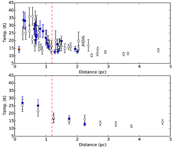
Figure 15: Clump temperature as a function of projected distance, in pc, to OS1a, the most luminous star in the W40 complex. The upper plot shows all clump individually plotted. The lower plot shows the mean temperature (and uncertainty) of clumps in 0.5 pc bins. In both plots filled markers represent protostellar clumps whereas hollow markers represent starless clumps. W40-SMM 19 is considered anomalous and its data are flagged as a red point. Red lines mark the partition between clump temperature regimes.

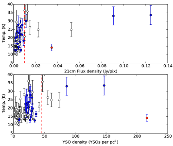
Figure 16: Clump temperature as a function of: (upper) mean VLA 21 cm flux detected in the area of each clump; and (lower) YSO surface density. In both plots, filled markers represent protostellar clumps whereas hollow markers represent starless clumps. W40-SMM 19 is considered anomalous and its data are flagged as a red point. Red lines mark the partition between clump temperature regimes.

Table 7: Dense cores in the W40 complex.

Clump ID	Regiona	Diameterb	Densityc	Proto-	M/MJ
(W40-SMM)		(pc)	(cm-3)	stars
1	E-DA	0.20	1.2$\times$105	4	0.6$\pm$0.2
2	W-DA	0.14	1.5$\times$105	-	0.8$\pm$0.2
3	W-DA	0.21	1.2$\times$105	1	1.1$\pm$0.3
4	W-DA	0.10	2.1$\times$105	1	0.4$\pm$0.1
5	E-DA	0.16	1.2$\times$105	1	0.4$\pm$0.1
6	W-DA	0.17	1.4$\times$105	1	0.8$\pm$0.2
8	W40-N	0.14	1.4$\times$105	1	1.0$\pm$0.2
9	W40-N	0.13	1.2$\times$105	-	0.6$\pm$0.2
10	ISO	0.16	1.7$\times$105	2	1.5$\pm$0.3
12	W40-N	0.13	1.8$\times$105	-	1.0$\pm$0.2
15	W40-S	0.13	2.0$\times$105	-	1.1$\pm$0.2
16	ISO	0.15	2.6$\times$105	-	2.3$\pm$0.4
18	W40-S	0.09	2.1$\times$105	-	1.0$\pm$0.2
20	W40-N	0.10	1.1$\times$105	-	0.3$\pm$0.1
22	ISO	0.1	1.7$\times$105	n/ad	1.0$\pm$0.2
26	W40-S	0.08	1.5$\times$105	-	0.4$\pm$0.1
28	ISO	0.05	3.9$\times$105	n/ad	0.9$\pm$0.2
29	ISO	0.04	3.3$\times$105	1	0.7$\pm$0.1
30	ISO	0.08	1.3$\times$105	-	0.6$\pm$0.1
33	ISO	0.10	1.2$\times$105	2	0.7$\pm$0.2
34	W40-N	0.09	1.2$\times$105	1	0.4$\pm$0.1
35	ISO	0.11	1.5$\times$105	-	1.8$\pm$0.4
37	ISO	0.09	1.2$\times$105	1	0.8$\pm$0.2
38	ISO	0.06	2.4$\times$105	-	0.8$\pm$0.2
43	ISO	0.04	2.5$\times$105	-	0.6$\pm$0.2
45	ISO	0.07	1.5$\times$105	1	0.6$\pm$0.1
47	W40-S	0.06	1.5$\times$105	-	0.3$\pm$0.1
52	ISO	0.04	1.1$\times$105	-	0.2$\pm$0.1
53	W40-N	0.03	1.1$\times$105	-	0.2$\pm$0.1
62	W40-N	0.04	1.1$\times$105	-	0.1$\pm$0.1

^a Region key: eastern Dust Arc (E-DA), western Dust Arc (W-DA), W40-N, W40-S and isolated clumps (ISO).
^b Flux weighted effective diameter as calculated by the clump-finding algorithm fellwalker (values were not deconvolved with respect to the JCMT beam).
^c The average volume density of a dense core along the line of sight. Each observation is a lower limit as effective size of the cloud is typically larger than a core. A dense core is defined where the density limit is greater than 10⁵ cm^-3, a value five times greater than the typical density of a star forming filament (2$\times$10⁴ cm^-3, André et al. 2014) and where the gas and dust temperatures are well coupled (Goldsmith, 2001).
^d Clumps beyond the coverage of our composite YSO catalogue.

6.4 YSO distribution

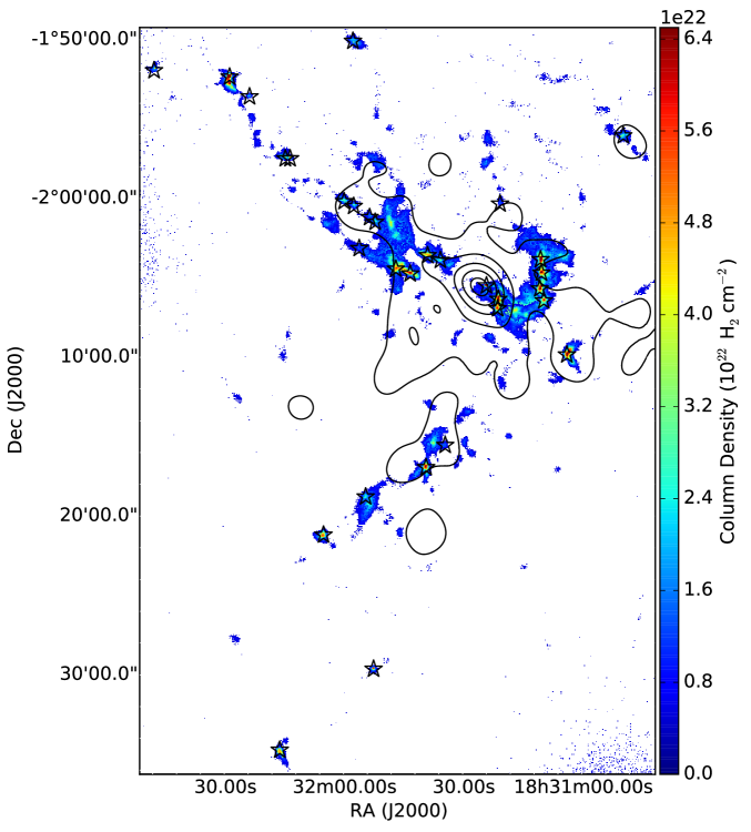
Figure 17: SCUBA-2 column density map of the W40 complex. Column density is shown for areas where emission is detected at or above S/N = 3 at 850 $\micron$. Column density is calculated using temperatures as presented in Figure 10 where available and a constant value of 15 K where a derived temperature is not. Contours describe YSO surface density with levels at 20, 60, 110, 160 and 210 YSO pc². Stars mark the location of each dense core identified in Table 7.

In this section we consider the YSO distribution based on the composite YSO catalogue produced from the SGBS list merged with the catalogues published by Kuhn et al. (2010), Rodríguez et al. (2010), Maury et al. (2011) and Mallick et al. (2013) (see Section 2.3 for full details). The locations of YSOs in our composite catalogue are plotted in Figure 20 with Class 0/I protostars and Class II/III PMS-stars denoted separately.

The YSO distribution was mapped by convolving the YSO positions with a 2^′ FWHM Gaussian to produce a surface density map with units of YSOs pc^-2 as shown in Figure 17. The stellar cluster is visible in Figure 17 and has a FWHM size of approximately 3.5^′$\times$ 2.5^′. The Dust Arc has its eastern end located towards the centre of the star cluster where the density peaks at 232 YSOs pc^-2. However, this value quickly drops off to 20 YSOs pc^-2 at its western edge near W40-SMM 31.

An increase in clump temperatures is also observed when the YSO surface density is greater than 45 YSO pc^-2 (Figure 16 lower, marked). Our YSO surface density map does not distinguish between embedded protostars and free-floating PMS-stars and therefore the YSO densities will be over-estimates of the densities of objects embedded within clumps. Given these uncertainties, we conclude that the radiative feedback from OS1a is dominating over any potential heating by the embedded YSO within this region.

The absolute number of protostars located within each clump was recorded. A total of 21/82 clumps have at least one Class 0/I protostar. Figure 14 shows how the distribution of clumps with protostars, compared to those without, is shifted to greater values in mass (5.5$\pm$1.3 from 2.0$\pm$0.6 M_⊙), column density (49$\pm$11 from 26$\pm$7$\times$10²¹ H₂ cm^-2), temperature (21$\pm$3 from 18$\pm$3 K) and M₈₅₀/M_J (0.6$\pm$0.2 from 0.4$\pm$0.1). These results are consistent with those of Foster et al. (2009) who observed that protostellar clumps appear warmer, more massive and more dense than starless clumps in Perseus.

For all cases in Figure 14, a threshold is observed, below which protostars are not found in clumps. These results argue that more massive, dense clumps are more likely to be unstable and contain a Class 0/I object. They also suggest that these clumps may be warmer, though the significant overlap in the temperature range renders this result inconclusive.

7 Evidence for radiative heating

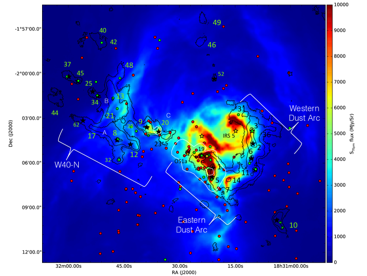
Figure 20: Archival Herschel 70 $\micron$ flux density map of the W40 complex (colour scale). Morphological features of W40-N and the Dust Arc are labelled alongside major clumps detected in SCUBA-2 850 $\micron$ emission (see Figure 13 for accurate clump positions). Black contours show SCUBA-2 850 $\micron$ at the 5 $\sigma$, 15 $\sigma$ and 50 $\sigma$ level. White contours show archival VLA 21 cm emission at 5 $\sigma$ and 25 $\sigma$ (Condon & Kaplan, 1998). The four OB stars OS1a, 2a, 3a and IRS 5 are marked as yellow stars. YSOs from our composite catalogue are displayed. Protostars (Class 0/I) are marked as green and PMS-stars (Class II/III) are marked as red. Dense cores identified in Table 7 are marked as black stars in their associated clump.

The W40 complex contains OB stars that radiate photons with sufficient energy to heat and ionise a portion of the ISM. Direct evidence of this heating is observed in the dust temperature maps presented and discussed in Sections 5 and 6.

The most prominent heating in the W40 complex occurs along the eastern Dust Arc, a very complex region of star-formation running from W40-SMM 19 to 14, and is the direct result of external heating from the nearby OS1a. The O9.5v star is primarily responsible for a mean clump temperature of 35$\pm$6 K in this filament. By comparison, a number of isolated clumps, with or without protostars, found well outside of the nebulosity have a mean temperature of 15 K, consistent with those derived for cores in Perseus using Bonnor-Ebert models (Johnstone et al. 2000, Kirk et al. 2006). Bright free-free emission observed in the eastern Dust Arc, as shown in Figures 6 and 9, is considered evidence of an interaction between the eastern Dust Arc and the H ii region. Figure 21 shows a possible configuration for this interaction.

The western Dust Arc leads from W40-SMM 31 southeast towards W40-SMM 11, and includes the B1 star IRS 5 which appears to be producing a secondary nebulosity visible in Herschel 70 $\micron$ data (Figure 20) that is consistent with H$\alpha$ emission (Mallick et al. 2013). A population of Class 0/I protostars is observed in the western Dust Arc by Maury et al. (2011), some of which coincide with dense cores W40-SMM 2, 3, 4, and 6. This filament lies well outside of the main stellar cluster associated with OS1a and has a YSO density of 22 YSO pc^-2 which is comparable to W40-N. We observe a mean clump temperature of 26$\pm$3 K for the western Dust Arc. Though this is warmer than the average clump in the W40 complex, it is notably cooler that the eastern Dust Arc (35$\pm$6 K).

Shimoikura et al. (2015) argues that the western Dust Arc is a shell of material forming around the H ii region of OS1a. However, our temperature maps lead us to believe that the Dust Arc is located significantly outside of the H ii region as we do not observe heating and free-free emission along its length to the extent of that observed in the eastern Dust Arc. Figure 21 presents a schematic layout of the W40 complex in RA/Dec/Line-of-sight space (by assimilating 3D information from the CO maps presented by us and Shimoikura et al. 2015, and the distance measurements of Shuping et al. 2012).

Evidence from the Serpens MWC 297 region suggests that radiative heating from a primary generation of high-mass stars can raise clump temperature, and potentially suppress any subsequent star-formation in the neighbouring clumps (Rumble et al., 2015). In Section 6.3 we have shown how heating from OS1a in the eastern Dust Arc is making these clumps, in particular W40-SMM 14, more stable to gravitational collapse (due to the increase of thermal support) than those in the western Dust Arc. By increasing the Jeans mass, the heating has the potential to skew the initial mass function to larger masses. However, as none of the clumps in the eastern Dust Arc have sufficient mass to exceed their enlarged Jeans mass, fragmentation under gravitational collapse is less likely to occur and the star formation rate may be suppressed. Given the continued radiative feedback from OS1a/expansion of the H ii region, it seems unlikely that clumps in the eastern Dust Arc will cool sufficiently to allow self-gravity to overwhelm thermal support and fragmentation to occur. We therefore conclude that it is likely that the eastern Dust Arc is less active in star-formation than the western Dust Arc.

In addition to the OB stars, there is an association of low-mass PMS-stars, observed by Kuhn et al. (2010), that also produces photons that may further externally heat the ISM. However, it is not possible to draw conclusions about the general significance of this mechanism given the dominance of the OB star heating in this region.

Addressing internal sources of radiative feedback, and their influence on the ISM, requires an assessment of embedded star formation occurring within the clumps. The majority of Class 0/I YSOs, presented in Figure 20, are associated with SCUBA-2 dust emission. Those associated with a local peak are Class 0/I protostars and those aside from a local peak are either very low-mass protostars or potentially mis-identified (due to IR contamination from the OB association or additional dust along the line-of-sight) PMS-stars. Those protostars found outside of SCUBA-2 850 $\micron$ 5$\sigma$ emission level are considered to be misidentified: false detections or edge-on disks (Heiderman & Evans, 2015). Considering clumps containing protostars (21$\pm$3 K) compared to those without protostars (18$\pm$3 K), we find there is no significant difference between the mean temperatures of the two populations (within the uncertainties). Figure 15 shows how this trend is independent of distance from OS1a, though we note that some of the temperatures calculated for distances less than 1.2 pc are likely influenced by OS1a.

We consider the specific case of OS2b. The B4 star appears embedded in the tip of W40-SMM1 (see Figures 8 and 20), where a peak in SCUBA-2 emission at 450 and 850 $\micron$ is detected, suggesting that we are observing a Class 0/I YSO. The temperature at the position of OS2b is 21$\pm$2 K (insert Figure 10). This value is comparable to the mean temperature of the dense cores in the Dust Arc (21 K, W40-SMM1, 2, 3, 4, 5, 6). No significant variation in temperature is noted amongst this sample irregardless of whether or not they contain a protostar. These findings suggest there is no evidence that embedded stars, up to B4 in spectral type, significantly heat their immediate clump environment (given the resolution of JCMT and a constant $\beta$). This finding supports the conclusions of Foster et al. (2009) that mid-B or later type stars have a relatively weak impact on their environment.

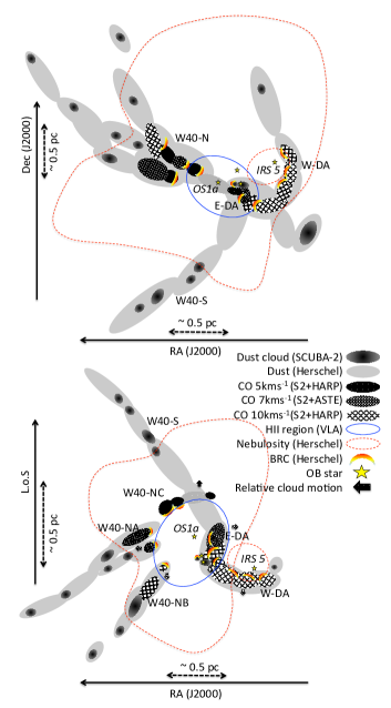
Figure 21: A schematic diagram of the location of clouds and features within the W40 complex. The upper figure represents the RA/Dec view of the Herschel/SCUBA-2 data presented in Figures 1 and 2 with cloud velocities observed by HARP and ASTE (Shimoikura et. al. 2015). Other features are explained in the key. The lower sketch shows the same region, this time viewed in line-of-sight vs RA space. The 5 km s^-1 blue-shifted clouds are considered to be on the far side of the expanding H ii bubble and at a further distance. Likewise the 10 km s^-1 red-shifted clouds are considered to be on the near side and at a closer distance. The 7 km s^-1 clouds observed by ASTE are taken to be moving perpendicular and at an intermediate distance. Where clouds have no velocity information, distance is inferred through attachment to clouds with a known distance. The location of the massive stars is given by Shuping et. al. (2012).

8 Summary and conclusions

We observed the W40 complex as part of the James Clerk Maxwell Telescope (JCMT) Gould Belt Survey (GBS) of nearby star-forming regions with SCUBA-2 at 450 and 850 $\micron$. The ¹²CO 3–2 line at 345.796 GHz was observed separately using HARP. The HARP data were used to subtract CO contributions to the SCUBA-2 850 $\micron$ map. In addition, archival radio data from Condon & Kaplan (1998) and Rodríguez et al. (2010) were examined to assess the large- and small-scale free-free flux contributions to both SCUBA-2 bands from the high-mass stars in the W40 complex OB association.

We produced maps of dust temperature and column density and estimated the Jeans stability, M₈₅₀/M_J, of submillimetre clumps. In conjunction with a new composite YSO candidate catalogue, we probed whether dust heating is caused by internal or external sources and what implications this heating has for star-formation in the region. Throughout this paper we refer to the Dust Arc, W40-N, W40-S and isolated clumps as various morphological features of the W40 complex. A schematic layout of these features is presented in Figure 21.

In addition to the catalogues presented here, all of the reduced datasets analysed in this paper are available at Doi xxxx.

Our key results on the W40 complex are summarised as follows:

1. We find evidence for significant levels of ¹²CO 3–2 line emission in HARP data that contaminates the 850 $\micron$ band by between 3 and 10% of the flux seen in the majority of the filaments. In a minority of areas contamination reaches up to 20%. Removing the ¹²CO 3–2 contamination significantly increases the calculated dust temperatures, beyond the calculated uncertainties.

2. Free-free emission is observed on large and small scales. Large-scale emission from an existing H ii region (spectral index of $\alpha_{\mathrm{ff}}$ = -0.1) powered by the primary ionising star OS1a contributes 0.5% of the peak flux at 450 $\micron$ and 5% at 850 $\micron$. Small-scale emission from an UCH ii region around the Herbig star OS2a contributes 9 and 12% at 450 and 850 $\micron$, respectively. Free-free emission for both large and small-scale sources was found to have a non-negligible, if limited, impact on dust temperature, often within the calculated uncertainties.

3. 82 clumps were detected by fellwalker in the 850 $\micron$ data and 21 of these have at least one protostar embedded within them. Clump temperatures range from 10 to 36 K. The mean temperatures of clumps in the Dust Arc, W40-N and W40-S are 26$\pm$4, 21$\pm$4 and 17$\pm$3 K. The mean temperature of the isolated clumps is 15$\pm$2 K. This result is consistent with temperatures observed in Serpens MWC 297 (Rumble et al., 2015) and other Gould Belt regions (Sadavoy et al. 2010 and Chen et al. submitted).

4. We find that clump temperature correlates with proximity to OS1a and the H ii region. We conclude that external radiative heating from the OB association is raising the temperature of the clumps. There is no evidence that embedded protostars are internally heating the filaments, though external influences may be masking such heating. As a result, the eastern Dust Arc has exceptionally high temperatures (mean 35$\pm$5 K), Jeans masses (mean 17 M_⊙), and Jeans stable clouds (mean M/M_J = 0.43). Partial radiative heating of the Dust Arc (internally or externally) has likely influenced the evolution of star-formation in the filament, favouring it in the cooler west, and potentially suppressing it in the warmer east. Globally, we find the population of clumps within the nebulosity Sh2-64 are more stable, as a function of peak column density, than that outside.

The W40 complex represents a high-mass star-forming region with a significant cluster of evolved PMS-stars and filaments forming new protostars from dense, starless cores. The region is complex and requires careful study to appreciate which radiative sources, from external and internal, are heating clumps of gas and dust. The region is dominated by an OB association that is powering an H ii region. In the near future we can expect this H ii region to expand and envelop many surrounding filaments. Within a few Myrs, we expect OS1a to go supernova. This event will likely have a cataclysmic impact on star-formation within the region. Any filament mass that has not been converted into stars, or eroded by the H ii region, may be destroyed at this point, bringing an end to star-formation in the W40 complex in its current form.

9 Acknowledgements

The JCMT has historically been operated by the Joint Astronomy Centre on behalf of the Science and Technology Facilities Council of the United Kingdom, the National Research Council of Canada and the Netherlands Organisation for Scientific Research. Additional funds for the construction of SCUBA-2 were provided by the Canada Foundation for Innovation. The authors thank the JCMT staff for their support of the GBS team in data collection and reduction efforts. The program under which the SCUBA-2 data used in this paper were taken is MJLSG33. This work was supported by a STFC studentship (Rumble) and the Exeter STFC consolidated grant (Hatchell). The Starlink software (Currie et al., 2014) is supported by the East Asian Observatory. These data were reduced using a development version from December 2014 (version 516b455a). This research used the services of the Canadian Advanced Network for Astronomy Research (CANFAR) which in turn is supported by CANARIE, Compute Canada, University of Victoria, the National Research Council of Canada, and the Canadian Space Agency. This research made use of APLpy, an open-source plotting package for Python hosted at http://aplpy.github.com, and Matplotlib, a 2D graphics package used for Python for application development, interactive scripting, and publication-quality image generation across user interfaces and operating systems. Herschel is an ESA space observatory with science instruments provided by European-led Principal Investigator consortia and with important participation from NASA. We would like to thank James Di Francesco for his internal review of this manuscript.

10 Affiliations

²Jeremiah Horrocks Institute, University of Central Lancashire, Preston, Lancashire, PR1 2HE, UK
³NRC Herzberg Astronomy and Astrophysics, 5071 West Saanich Rd, Victoria, BC, V9E 2E7, Canada
⁴Astrophysics Group, Cavendish Laboratory, J J Thomson Avenue, Cambridge, CB3 0HE
⁵Kavli Institute for Cosmology, Institute of Astronomy, University of Cambridge, Madingley Road, Cambridge, CB3 0HA, UK
⁶Joint Astronomy Centre, 660 N. A‘ohōkū Place, University Park, Hilo, Hawaii 96720, USA
⁷Department of Physics and Astronomy, University of Victoria, Victoria, BC, V8P 1A1, Canada
⁸Department of Physics and Astronomy, University of Waterloo, Waterloo, Ontario, N2L 3G1, Canada  
⁹LSST Project Office, 933 N. Cherry Ave, Tucson, AZ 85719, USA
¹⁰Leiden Observatory, Leiden University, PO Box 9513, 2300 RA Leiden, The Netherlands
¹¹Max-Planck Institute for Astronomy, Königstuhl 17, 69117 Heidelberg, Germany
¹²School of Physics and Astronomy, Cardiff University, The Parade, Cardiff, CF24 3AA, UK
¹³European Southern Observatory (ESO), Garching, Germany
¹⁴Jodrell Bank Centre for Astrophysics, Alan Turing Building, School of Physics and Astronomy, University of Manchester, Oxford Road, Manchester, M13 9PL, UK
¹⁵Current address: Institute for Astronomy, ETH Zurich, Wolfgang-Pauli-Strasse 27, CH-8093 Zurich, Switzerland
¹⁶Université de Montréal, Centre de Recherche en Astrophysique du Québec et département de physique, C.P. 6128, succ. centre-ville, Montréal, QC, H3C 3J7, Canada
¹⁷James Madison University, Harrisonburg, Virginia 22807, USA
¹⁸School of Physics, Astronomy & Mathematics, University of Hertfordshire, College Lane, Hatfield, HERTS AL10 9AB, UK
¹⁹Astrophysics Research Institute, Liverpool John Moores University, Egerton Warf, Birkenhead, CH41 1LD, UK
²⁰Imperial College London, Blackett Laboratory, Prince Consort Rd, London SW7 2BB, UK
²¹Dept of Physics & Astronomy, University of Manitoba, Winnipeg, Manitoba, R3T 2N2 Canada
²²Dunlap Institute for Astronomy & Astrophysics, University of Toronto, 50 St. George St., Toronto ON M5S 3H4 Canada
²³Dept. of Physical Sciences, The Open University, Milton Keynes MK7 6AA, UK
²⁴The Rutherford Appleton Laboratory, Chilton, Didcot, OX11 0NL, UK.
²⁵UK Astronomy Technology Centre, Royal Observatory, Blackford Hill, Edinburgh EH9 3HJ, UK
²⁶Institute for Astronomy, Royal Observatory, University of Edinburgh, Blackford Hill, Edinburgh EH9 3HJ, UK
²⁷Centre de recherche en astrophysique du Québec et Département de physique, de génie physique et d’optique, Université Laval, 1045 avenue de la médecine, Québec, G1V 0A6, Canada
²⁸Department of Physics and Astronomy, UCL, Gower St, London, WC1E 6BT, UK
²⁹Department of Physics and Astronomy, McMaster University, Hamilton, ON, L8S 4M1, Canada
³⁰Department of Physics, University of Alberta, Edmonton, AB T6G 2E1, Canada
³¹Max Planck Institute for Astronomy, Königstuhl 17, D-69117 Heidelberg, Germany
³²University of Western Sydney, Locked Bag 1797, Penrith NSW 2751, Australia
³³National Astronomical Observatory of China, 20A Datun Road, Chaoyang District, Beijing 100012, China

Appendix A SCUBA-2 data

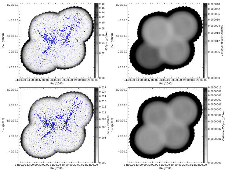
Figure 22: SCUBA-2 IR2 reductions of Aquila region (east the W40 complex, west Serpens South) featuring data and variance maps at 450 and 850 $\micron$. Contours show the outline of the SCUBA-2 external mask used in the reduction process.

Figure 22 shows complete SCUBA-2 450 and 850 $\micron$ mosaics that include the W40 complex and the neighbouring Serpens South region (not considered to be physically connected to W40 complex). In addition we also present variance maps for the observations where the four PONG of varying noise levels have been mosaiced together. Plotted on the data maps are the SCUBA-2 external mask that are outlined in Section 2.

Appendix B Method for temperature maps

A convolution kernel, $K\left(A\Rightarrow B\right)$, is constructed from an analytical beam map or published beam model such that a point spread function (PSF_A) is mapped onto a PSF_B. Full details of the application of the kernel are given in Aniano et al. (2011) and Pattle et al. (2015).

The post-CO and free-free subtracted SCUBA-2 450 $\micron$ map is convolved to the resolution of the 850 $\micron$ map using the SCUBA-2 convolution kernel using analytical beam map PSFs (Dempsey et al., 2013). Pre- and post-convolution kernel maps are prepared to ensure a common pixel grid and clipping at a level of 5 $\sigma$ at 450 $\micron$, the details of which are covered in more detail by Aniano et al. (2011). Ratio maps are then prepared by dividing 450 $\micron$ flux by 850 $\micron$ flux as in the form of Equation 3. Further details of these steps are discussed in Rumble et al. (2015).

Noise on the input maps is propagated through the flux ratio algorithm to calculate the error per pixel on the temperature. Rumble et al. (2015) calculate this solution analytically for their dual-beam cross-convolution method. Here, we calculate uncertainty through a Monte-Carlo process. Namely, random numbers are generated from a Gaussian distribution of width $\sigma_{\mathrm{input}}$, equivalent to the noise level of the map. Each number is added to a unique pixel on an otherwise flat 450 $\micron$ map. The input maps are then convolved through the kernel algorithm and the spread of the distribution of pixels across the output map, $\sigma_{\mathrm{output}}$, is measured to recover the propagated uncertainty.

A cut on temperature is made based on the propagated uncertainties. Pixels where the fractional error is greater than one standard deviation of a normal distribution were considered bad. This criterion had the effect at removing uncertain edge pixels (a known problem with this method; see Rumble et al. 2015).

We find that the ratio uncertainties produced by the kernel method of Aniano et al. (2011) and Pattle et al. (2015) are systematically higher than those produced by the dual-beam method in Rumble et al. (2015) by a factor of approximately two. Increasing resolution inevitably increases uncertainty as the beam area samples fewer data points. The ratio of beam areas between the kernel method (14.8^′′) and the dual-beam method (19.9^′′) is 1.9, consistent with the observations. Appendix B (Figure 23) shows that, despite the increase in uncertainty, the absolute values of the dust flux ratios calculated by the two methods are found to be comparable with a Pearson-correlation co-efficent of 96%.

We therefore conclude that the two methods produce consistent results for ratio and temperature, with the kernel method improving the resolution at the expense of the error in the results.

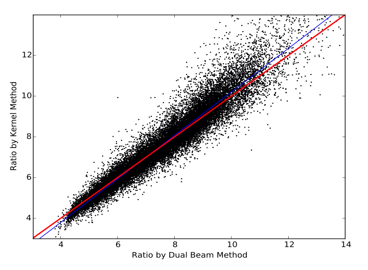
Figure 23: Comparison of the pixel flux ratio values from the dual beam and kernel convolution methods. The blue line shows a linear regression fit to the distribution with a Pearson-correlation coefficient of 96% to parity (red line).

Appendix C Spatial filtering

Spatial filters necessary to reduce excess large-scale structure in the SCUBA-2 reductions were applied to the data using the cupid tool findback (Berry et al. 2007, Berry et al. 2013). This tool works by twice filtering pixels (firstly to a minimum and secondly a maximum value) with respect to those pixels within a pre-defined spatial scale or ‘box’ parameter which we refer to as the filter size. Using this method a lower envelope of the data is estimated.

The results of tests of various filter sizes are presented in Figure 24, alongside the unfiltered data, as the distribution of flux ratios for a control area of the W40 complex (W40-N). Larger filters were found to maximise the number of pixels in the data at the expense of excessive flux ratios. We set a criterion for the ideal filter that was a compromise between the highest absolute number of pixels retained (post filtering and 5 $\sigma$ cut), in a sample area of the map and the lowest percentage of ‘bad’ pixels (ratios higher than 9.5). A scale size of 4^′ is the optimum solution with 5.7% of pixels returning unphysical ratios (down from 28.8% in the unfiltered data). See Section 4 for details of how flux ratio is calculated. The filtered maps of the W40 complex are shown in Figure 2.

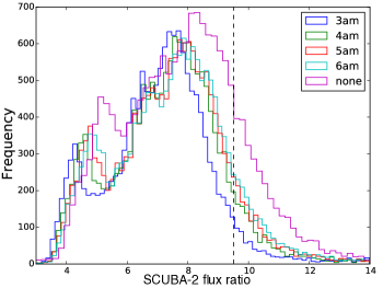
Figure 24: Histograms of flux ratio for the Aquila CO subtracted SCUBA-2 reductions with varying spatial filters applied. Filter sizes, in arcminutes, are labelled on the plot. The flux ratios calculated with no filter are also included for comparison. Histograms are examined for total volume below 9.5, an arbitrary value above which ratios are considered unphysical.

Appendix D Temperature method comparison

As outlined in Section 5, the degeneracy between temperature and $\beta$ can be removed with the inclusion of additional submillimeter wavelengths and through the fitting of a SED model to the data to independently determine these free parameters. Herschel SPIRE and PACS bands have been used by Bontemps et al. (2010), Könyves et al. (2010) and Könyves et al. (2015) to calculate temperatures in the Aquila region using this method.

SCUBA-2 bands have been incorporated alongside Herschel bands to improve completeness at longer wavelengths by Sadavoy et al. (2013) and Chen et al. (2016). The SCUBA-2 data reduction process explicitly filters large-scale structure that may trace lower density, warmer material so that dense cores and filaments can be targeted. This large-scale structure is retained in Herschel observations. Sadavoy et al. (2013) outlines additional spatial filtering and corrections to be made to Herschel images so that they can be combined with SCUBA-2 images.

Incorporating additional wavelengths requires all the data to take the lowest common resolution. Using all available Herschel bands requires a common resolution of 36.4^′′ associated with the 500 $\micron$ band. At this resolution, analysis is limited to a general overview of temperatures in the region. The 14.6^′′ resolution achieved using the SCUBA-2 450/850 $\micron$ flux ratio method (as outlined in Appendix B) allows temperatures to be studied down to the length scale of a protostellar core (0.05 pc, Rygl et al. 2013) under the assumption of constant $\beta$.

By using a more complete spectral range, SED fitting can discern multiple temperature cloud components in a way that the ratio method cannot. Should a target contain both hot ($\sim$50 K or greater) and cold ($\sim$15 K) cloud components, emission from the hot dust can dominate emission at shorter wavelengths (70 and 160 $\micron$) at even a small fraction of the mass of the cold component, as illustrated in Figure 25. Fitting only the wavelengths longwards of the SED peak will preferentially sample the colder cloud components that dominate in mass (Shetty et al., 2009). The SCUBA-2 450/850 $\micron$ flux ratio is well positioned on the SED to measure the temperature of these colder components for the purposes of calculating their Jeans masses.

Appendix E Clumpfinding analysis

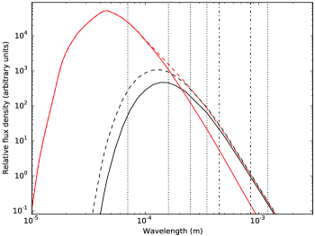
Figure 25: Model opacity-modified blackbody SEDs for a cold (black, 15 K) cloud and a hot (grey, red online, 50 K) cloud with 3% of the mass of the cold cloud. The red dashed SED represents the two cloud components combined and the black dashed SED represents how the combined SED resembles a single 17 K cloud at SCUBA-2 450 and 850 $\micron$ bands (dot-dashed vertical lines). The Herschel 70, 160, 250 and 350 $\micron$ bands, and the MAMBO 1.2 mm band are also marked (dotted vertical lines). Note how the 50 K component dominates the fluxes at 70 and 160 microns.

We use the clump-finding algorithm fellwalker (Berry, 2015) to extract a catalogue of irregular clumps from the SCUBA-2 850 $\micron$ data (Figure 2). Each clump then forms the basis of a mask for the temperature map (Figure 10) so that a single clump temperature can be found and used to calculate various additional properties.

Details of how we apply fellwalker to SCUBA-2 data are given in Rumble et al. (2015). Briefly, by setting the parameter MinDip = 3$\sigma$, fellwalker is tuned to break up large-scale continuous clouds with multiple bright cores into discrete clumps. Also, the Noise and MinHeight parameters are set to 5 $\sigma$ and MaxJump is set to one pixel ensuring that all extracted clumps are significant detections but allowing for fragmentation peaks. Beam deconvolution of clump sizes was set to false. However, the flux weighted beam sizes were calculated using a FWHMbeam parameter of 1 pixel, or 3^′′. This was found to be equivalent to the FWHM given high SNR. At low SNR (less than 10) fellwalker will underestimate the size of the clump. A reduced beam size was used to ensure that point-like sources, such as isolated protostellar envelopes or discs, were not omitted by the algorithm. Finally, by setting MinPix to four pixels, a large number of single-pixel objects that were likely noise artefacts were removed from the catalogue.

The original observations also include objects that are part of Serpens South which is located near to the W40 complex on the sky. There is no physically defined point in the SCUBA-2 data that describes where the W40 complex ends and Serpens South begins and so we define an arbitrary cut off along the meridian RA(J2000) = 18:30:40 with all objects eastward belonging to the W40 complex and westward to Serpens South. Whilst this approach may risk associating some clumps with the wrong region, we estimate this will affect less than 5% of members overall.

References

- André et al. (2014) André P., Di Francesco J., Ward-Thompson D., Inutsuka S.-I., Pudritz R. E., Pineda J. E., 2014, Protostars and Planets VI, pp 27–51
- André et al. (2010) André P., Men’shchikov A., Bontemps S., Könyves V., Motte F., Schneider N., Didelon P., Minier V., Saraceno P., Ward-Thompson D., 2010, A&A, 518, L102
- Aniano et al. (2011) Aniano G., Draine B. T., Gordon K. D., Sandstrom K., 2011, PASP, 123, 1218
- Arzoumanian et al. (2011) Arzoumanian D., André P., Didelon P., Könyves V., Schneider N., Men’shchikov A., 2011, A&A, 529, L6
- Bate (2009) Bate M. R., 2009, MNRAS, 392, 1363
- Beckwith et al. (1990) Beckwith S. V. W., Sargent A. I., Chini R. S., Guesten R., 1990, AJ, 99, 924
- Berry (2015) Berry D. S., 2015, Astronomy and Computing, 10, 22
- Berry et al. (2007) Berry D. S., Reinhold K., Jenness T., Economou F., 2007, in Shaw R. A., Hill F., Bell D. J., eds, Astronomical Data Analysis Software and Systems XVI Vol. 376 of Astronomical Society of the Pacific Conference Series, CUPID: A Clump Identification and Analysis Package. p. 425
- Berry et al. (2013) Berry D. S., Reinhold K., Jenness T., Economou F., , 2013, CUPID: Clump Identification and Analysis Package
- Bertoldi & McKee (1992) Bertoldi F., McKee C. F., 1992, ApJ, 395, 140
- Bontemps et al. (2010) Bontemps S., André P., Könyves V., Men’shchikov A., Schneider N., Maury A., Peretto N., Arzoumanian D., Attard M., Motte F., Minier V., 2010, A&A, 518, L85
- Buckle et al. (2015) Buckle J. V., Drabek-Maunder E., Greaves J., Richer J. S., Matthews B. C., Johnstone D., Kirk H., 2015, MNRAS, 449, 2472
- Buckle et al. (2009) Buckle J. V., Hills R. E., Smith H., Dent W. R. F., Bell G., Curtis E. I., Dace R., Gibson H., Graves S. F., Leech J., Richer J. S., Williamson R., Withington S., Yassin G., 2009, MNRAS, 399, 1026
- Calvet & Gullbring (1998) Calvet N., Gullbring E., 1998, ApJ, 509, 802
- Canto et al. (1984) Canto J., Rodriguez L. F., Calvet N., Levreault R. M., 1984, ApJ, 282, 631
- Chapin et al. (2013) Chapin E. L., Berry D. S., Gibb A. G., Jenness T., Scott D., Tilanus R. P. J., Economou F., Holland W. S., 2013, MNRAS, 430, 2545
- Condon & Kaplan (1998) Condon J. J., Kaplan D. L., 1998, VizieR Online Data Catalog, 211, 70361
- Cunningham et al. (1994) Cunningham C. R., Gear W. K., Duncan W. D., Hastings P. R., Holland W. S., 1994, in Crawford D. L., Craine E. R., eds, Instrumentation in Astronomy VIII Vol. 2198 of Society of Photo-Optical Instrumentation Engineers (SPIE) Conference Series, SCUBA: the submillimeter common-user bolometer array for the James Clerk Maxwell Telescope. pp 638–649
- Currie et al. (2014) Currie M. J., Berry D. S., Jenness T., Gibb A. G., Bell G. S., Draper P. W., 2014, in Manset N., Forshay P., eds, Astronomical Data Analysis Software and Systems XXIII Vol. 485 of Astronomical Society of the Pacific Conference Series, Starlink Software in 2013. p. 391
- Dame et al. (2001) Dame T. M., Hartmann D., Thaddeus P., 2001, ApJ, 547, 792
- Davis et al. (2000) Davis C. J., Dent W. R. F., Matthews H. E., Coulson I. M., McCaughrean M. J., 2000, MNRAS, 318, 952
- Davis et al. (1999) Davis C. J., Matthews H. E., Ray T. P., Dent W. R. F., Richer J. S., 1999, MNRAS, 309, 141
- Deharveng et al. (2012) Deharveng L., Zavagno A., Anderson L. D., Motte F., Abergel A., André P., Bontemps S., Leleu G., Roussel H., Russeil D., 2012, A&A, 546, A74
- Dempsey et al. (2013) Dempsey J. T., Friberg P., Jenness T., Tilanus R. P. J., Thomas H. S., Holland W. S., Bintley D., Berry D. S., Chapin E. L., Chrysostomou A., Davis G. R., Gibb A. G., Parsons H., Robson E. I., 2013, MNRAS, 430, 2534
- Dobashi et al. (2005) Dobashi K., Uehara H., Kandori R., Sakurai T., Kaiden M., Umemoto T., Sato F., 2005, PASJ, 57, 1
- Drabek et al. (2012) Drabek E., Hatchell J., Friberg P., Richer J., Graves S., Buckle J. V., Nutter D., Johnstone D., Di Francesco J., 2012, MNRAS, 426, 23
- Drew et al. (1997) Drew J. E., Busfield G., Hoare M. G., Murdoch K. A., Nixon C. A., Oudmaijer R. D., 1997, MNRAS, 286, 538
- Dunham et al. (2015) Dunham M. M., Allen L. E., Evans II N. J., Broekhoven-Fiene H., Cieza L. A., Di Francesco J., Gutermuth R. A., Harvey P. M., Hatchell J., Heiderman A., Huard T. L., Johnstone D., Kirk J. M., Matthews B. C., Miller J. F., Peterson D. E., Young K. E., 2015, ApJS, 220, 11
- Enoch et al. (2011) Enoch M. L., Corder S., Duchêne G., Bock D. C., Bolatto A. D., Culverhouse T. L., Kwon W., Lamb J. W., Leitch E. M., Marrone D. P., Muchovej S. J., Pérez L. M., Scott S. L., Teuben P. J., Wright M. C. H., Zauderer B. A., 2011, ApJS, 195, 21
- Evans et al. (2009) Evans N. J. II., Dunham M. M., Jørgensen J. K., Enoch M. L., Merín B., van Dishoeck E. F., Alcalá J. M., Myers P. C., Stapelfeldt K. R., 2009, ApJS, 181, 321
- Foster et al. (2009) Foster J. B., Rosolowsky E. W., Kauffmann J., Pineda J. E., Borkin M. A., Caselli P., Myers P. C., Goodman A. A., 2009, ApJ, 696, 298
- Garay et al. (1996) Garay G., Ramirez S., Rodriguez L. F., Curiel S., Torrelles J. M., 1996, ApJ, 459, 193
- Goldreich & Kwan (1974) Goldreich P., Kwan J., 1974, ApJ, 189, 441
- Goldsmith (2001) Goldsmith P. F., 2001, ApJ, 557, 736
- Gordon et al. (2010) Gordon K. D., Galliano F., Hony S., 2010, A&A, 518, L89
- Gordon (1995) Gordon M. A., 1995, A&A, 301, 853
- Griffin et al. (2010) Griffin M. J., Abergel A., Abreu A., Ade P. A. R., André P., Augueres J.-L., Babbedge T., 2010, A&A, 518, L3
- Gutermuth et al. (2008) Gutermuth R. A., Bourke T. L., Allen L. E., Myers P. C., Megeath S. T., Matthews B. C., Jørgensen J. K., Di Francesco J., Ward-Thompson D., Huard T. L., Brooke T. Y., Dunham M. M., Cieza L. A., Harvey P. M., Chapman N. L., 2008, ApJ, 673, L151
- Harvey et al. (1979) Harvey P. M., Thronson Jr. H. A., Gatley I., 1979, ApJ, 231, 115
- Hatchell & Dunham (2009) Hatchell J., Dunham M. M., 2009, A&A, 502, 139
- Hatchell et al. (2005) Hatchell J., Richer J. S., Fuller G. A., Qualtrough C. J., Ladd E. F., Chandler C. J., 2005, A&A, 440, 151
- Hatchell et al. (2013) Hatchell J., Wilson T., Drabek E., Curtis E., Richer J., Nutter D., Di Francesco J., Ward-Thompson D., JCMT GBS Consortium 2013, MNRAS, 429, L10
- Heiderman & Evans (2015) Heiderman A., Evans II N. J., 2015, ApJ, 806, 231
- Hennebelle & Chabrier (2011) Hennebelle P., Chabrier G., 2011, ApJ, 743, L29
- Hildebrand (1983) Hildebrand R. H., 1983, QJRAS, 24, 267
- Holland et al. (2013) Holland W. S., Bintley D., Chapin E. L., Chrysostomou A., Davis G. R., Dempsey J. T., Duncan W. D., Fich M., Friberg P., Halpern M., Irwin K. D., Jenness T., Kelly B. D., MacIntosh M. J., Robson E. I., 2013, MNRAS, 430, 2513
- Hughes (1991) Hughes V. A., 1991, ApJ, 383, 280
- Hughes et al. (1995) Hughes V. A., Cohen R. J., Garrington S., 1995, MNRAS, 272, 469
- Jeans (1902) Jeans J. H., 1902, Royal Society of London Philosophical Transactions Series A, 199, 1
- Jenness et al. (2015) Jenness T., Currie M. J., Tilanus R. P. J., Cavanagh B., Berry D. S., Leech J., Rizzi L., 2015, MNRAS, 453, 73
- Johnstone et al. (2003) Johnstone D., Boonman A. M. S., van Dishoeck E. F., 2003, A&A, 412, 157
- Johnstone et al. (2000) Johnstone D., Wilson C. D., Moriarty-Schieven G., Joncas G., Smith G., Gregersen E., Fich M., 2000, ApJ, 545, 327
- Juvela et al. (2015) Juvela M., Demyk K., Doi Y., Hughes A., Lefèvre C., Marshall D. J., Meny C., Montillaud J., Pagani L., Paradis D., Ristorcelli I., Malinen J., Montier L. A., Paladini R., Pelkonen V.-M., Rivera-Ingraham A., 2015, A&A, 584, A94
- Kackley et al. (2010) Kackley R., Scott D., Chapin E., Friberg P., 2010, in Society of Photo-Optical Instrumentation Engineers (SPIE) Conference Series Vol. 7740 of Society of Photo-Optical Instrumentation Engineers (SPIE) Conference Series, JCMT Telescope Control System upgrades for SCUBA-2. p. 1
- Kauffmann et al. (2008) Kauffmann J., Bertoldi F., Bourke T. L., Evans II N. J., Lee C. W., 2008, A&A, 487, 993
- Kirk et al. (2006) Kirk H., Johnstone D., Di Francesco J., 2006, ApJ, 646, 1009
- Koenig et al. (2008) Koenig X. P., Allen L. E., Gutermuth R. A., Hora J. L., Brunt C. M., Muzerolle J., 2008, ApJ, 688, 1142
- Könyves et al. (2015) Könyves V., André P., Men’shchikov A., Palmeirim P., Arzoumanian D., Schneider N., Roy A., Didelon P., Maury A., Shimajiri Y., Di Francesco J., Bontemps S., Peretto N., 2015, A&A, 584, A91
- Könyves et al. (2010) Könyves V., André P., Men’shchikov A., Schneider N., Arzoumanian D., Bontemps S., Attard M., Motte F., Didelon P., 2010, A&A, 518, L106
- Kuhn et al. (2015) Kuhn M. A., Getman K. V., Feigelson E. D., 2015, ApJ, 802, 60
- Kuhn et al. (2010) Kuhn M. A., Getman K. V., Feigelson E. D., Reipurth B., Rodney S. A., Garmire G. P., 2010, ApJ, 725, 2485
- Kurtz et al. (1994) Kurtz S., Churchwell E., Wood D. O. S., 1994, ApJS, 91, 659
- Mairs et al. (2015) Mairs S., Johnstone D., Kirk H., Graves S., Buckle J., JCMT Gould Belt survey Team 2015, MNRAS, 454, 2557
- Mairs et al. (2014) Mairs S., Johnstone D., Offner S. S. R., Schnee S., 2014, ApJ, 783, 60
- Malbet et al. (2007) Malbet F., Benisty M., de Wit W.-J., Kraus S., Meilland A., Millour F., Tatulli E., Berger J.-P., Chesneau O., Hofmann K.-H., Isella A., Natta A., Petrov R. G., Preibisch T., Stee P., Testi L., Weigelt G., Antonelli P., Beckmann U., 2007, A&A, 464, 43
- Mallick et al. (2013) Mallick K. K., Kumar M. S. N., Ojha D. K., Bachiller R., Samal M. R., Pirogov L., 2013, ApJ, 779, 113
- Manoj et al. (2007) Manoj P., Ho P. T. P., Ohashi N., Zhang Q., Hasegawa T., Chen H.-R., Bhatt H. C., Ashok N. M., 2007, ApJ, 667, L187
- Mathis et al. (1983) Mathis J. S., Mezger P. G., Panagia N., 1983, A&A, 128, 212
- Matzner (2002) Matzner C. D., 2002, ApJ, 566, 302
- Maury et al. (2011) Maury A. J., André P., Men’shchikov A., Könyves V., Bontemps S., 2011, A&A, 535, A77
- Men’shchikov et al. (2010) Men’shchikov A., André P., Didelon P., Könyves V., Schneider N., Motte F., Bontemps S., Arzoumanian D., Attard M., Abergel A., Baluteau J.-P., Bernard J.-P., Cambrésy L., 2010, A&A, 518, L103
- Mezger & Henderson (1967) Mezger P. G., Henderson A. P., 1967, ApJ, 147, 471
- Mitchell et al. (2001) Mitchell G. F., Johnstone D., Moriarty-Schieven G., Fich M., Tothill N. F. H., 2001, ApJ, 556, 215
- Offner et al. (2009) Offner S. S. R., Klein R. I., McKee C. F., Krumholz M. R., 2009, ApJ, 703, 131
- Olnon (1975) Olnon F. M., 1975, A&A, 39, 217
- Ortiz-León et al. (2015) Ortiz-León G. N., Loinard L., Mioduszewski A. J., Dzib S. A., Rodríguez L. F., 2015, ApJ, 805, 9
- Ossenkopf & Henning (1994) Ossenkopf V., Henning T., 1994, A&A, 291, 943
- Oster (1961) Oster L., 1961, ApJ, 134, 1010
- Panagia & Felli (1975) Panagia N., Felli M., 1975, A&A, 39, 1
- Pattle et al. (2015) Pattle K., Ward-Thompson D., Kirk J. M., White G. J., Drabek-Maunder E., 2015, MNRAS, 450, 1094
- Pirogov et al. (2013) Pirogov L., Ojha D. K., Thomasson M., Wu Y.-F., Zinchenko I., 2013, MNRAS, 436, 3186
- Planck Collaboration et al. (2011) Planck Collaboration Ade P. A. R., Aghanim N., Arnaud M., Ashdown M., Aumont J., Baccigalupi C., Balbi A., Banday A. J., Barreiro R. B., et al. 2011, A&A, 536, A23
- Radhakrishnan et al. (1972) Radhakrishnan V., Goss W. M., Murray J. D., Brooks J. W., 1972, ApJS, 24, 49
- Reid & Wilson (2005) Reid M. A., Wilson C. D., 2005, ApJ, 625, 891
- Reynolds (1986) Reynolds S. P., 1986, ApJ, 304, 713
- Robitaille & Whitney (2014) Robitaille T. P., Whitney B. A., 2014, in Stamatellos D., Goodwin S., Ward-Thompson D., eds, Advances in Solid State Physics Vol. 36 of Advances in Solid State Physics, A New Set of Model Spectral Energy Distributions for Young Stellar Objects. p. 157
- Rodney & Reipurth (2008) Rodney S. A., Reipurth B., 2008, The W40 Cloud Complex. p. 683
- Rodríguez et al. (2010) Rodríguez L. F., Rodney S. A., Reipurth B., 2010, AJ, 140, 968
- Rumble et al. (2015) Rumble D., Hatchell J., Gutermuth R. A., Kirk H., Buckle J., Beaulieu S. F., Berry D. S., Broekhoven-Fiene H., 2015, MNRAS, 448, 1551
- Rygl et al. (2013) Rygl K. L. J., Benedettini M., Schisano E., Elia D., Molinari S., Pezzuto S., André P., Bernard J. P., White G. J., Polychroni D., Bontemps S., Cox N. L. J., Di Francesco J., 2013, A&A, 549, L1
- Sadavoy et al. (2010) Sadavoy S. I., Di Francesco J., Bontemps S., Megeath S. T., Rebull L. M., Allgaier E., Carey S., Gutermuth R., Hora J., Huard T., McCabe C.-E., Muzerolle J., Noriega-Crespo A., Padgett D., Terebey S., 2010, ApJ, 710, 1247
- Sadavoy et al. (2013) Sadavoy S. I., Di Francesco J., Johnstone D., Currie M. J., Drabek E., Hatchell J., Nutter D., André P., Arzoumanian D., Benedettini M., 2013, ApJ, 767, 126
- Salji et al. (2015) Salji C. J., Richer J. S., Buckle J. V., Francesco J. D., Hatchell J., Hogerheijde M., Johnstone D., Kirk H., Ward-Thompson D., JCMT GBS Consortium 2015, MNRAS, 449, 1782
- Sandell et al. (2011) Sandell G., Weintraub D. A., Hamidouche M., 2011, ApJ, 727, 26
- Sharpless (1959) Sharpless S., 1959, ApJS, 4, 257
- Shetty et al. (2009) Shetty R., Kauffmann J., Schnee S., Goodman A. A., 2009, ApJ, 696, 676
- Shetty et al. (2009) Shetty R., Kauffmann J., Schnee S., Goodman A. A., Ercolano B., 2009, ApJ, 696, 2234
- Shetty et al. (2015) Shetty R., Roman-Duval J., Hony S., Cormier D., Klessen R. S., Konstandin L. K., Loredo T., Pellegrini E. W., Ruppert D., 2015, ArXiv e-prints:1509.00639
- Shimoikura et al. (2015) Shimoikura T., Dobashi K., Nakamura F., Hara C., Tanaka T., Shimajiri Y., Sugitani K., Kawabe R., 2015, ApJ, 806, 201
- Shirley et al. (2002) Shirley Y. L., Evans N. J., Rawlings J. M. C., 2002, ApJ, 575, 337
- Shirley et al. (2000) Shirley Y. L., Evans N. J., Rawlings J. M. C., Gregersen E. M., 2000, ApJS, 131, 249
- Shuping et al. (2012) Shuping R. Y., Vacca W. D., Kassis M., Yu K. C., 2012, AJ, 144, 116
- Skinner et al. (1993) Skinner S. L., Brown A., Stewart R. T., 1993, ApJS, 87, 217
- Smith et al. (1985) Smith J., Bentley A., Castelaz M., Gehrz R. D., Grasdalen G. L., Hackwell J. A., 1985, ApJ, 291, 571
- Straižys et al. (2003) Straižys V., Černis K., Bartašiūtė S., 2003, A&A, 405, 585
- Tielens & Hollenbach (1985) Tielens A. G. G. M., Hollenbach D., 1985, ApJ, 291, 722
- Tothill et al. (2002) Tothill N. F. H., White G. J., Matthews H. E., McCutcheon W. H., McCaughrean M. J., Kenworthy M. A., 2002, ApJ, 580, 285
- Vallee & MacLeod (1991) Vallee J. P., MacLeod J. M., 1991, A&A, 250, 143
- van der Wiel et al. (2014) van der Wiel M. H. D., Naylor D. A., Kamp I., Ménard F., Thi W.-F., Woitke P., Olofsson G., Pontoppidan K. M., Di Francesco J., Glauser A. M., Greaves J. S., Ivison R. J., 2014, MNRAS, 444, 3911
- Ward-Thompson et al. (2007) Ward-Thompson D., Di Francesco J., Hatchell J., Hogerheijde M. R., Nutter D., Bastien P., Basu S., Bonnell I., Bowey J., Brunt C., Buckle J., 2007, PASP, 119, 855
- Westerhout (1958) Westerhout G., 1958, A&A, 14, 215
- Wright & Barlow (1975) Wright A. E., Barlow M. J., 1975, MNRAS, 170, 41
- Zeilik & Lada (1978) Zeilik II M., Lada C. J., 1978, ApJ, 222, 896
- Zhu et al. (2006) Zhu L., Wu Y.-F., Wei Y., 2006, 6, 61
- Ziener & Eislöffel (1999) Ziener R., Eislöffel J., 1999, A&A, 347, 565