Improving fast generation of halo catalogs with higher-order Lagrangian perturbation theory

Abstract

We present the latest version of pinocchio, a code that generates catalogues of DM haloes in an approximate but fast way with respect to an N–body simulation. This code version extends the computation of particle and halo displacements up to 3rd-order Lagrangian Perturbation Theory (LPT), in contrast with previous versions that used Zeldovich approximation (ZA).

We run pinocchio on the same initial configuration of a reference N–body simulation, so that the comparison extends to the object–by–object level. We consider haloes at redshifts $0$ and $1$, using different LPT orders either for halo construction - where displacements are needed to decide particle accretion onto a halo or halo merging - or to compute halo final positions.

We compare the clustering properties of pinocchio haloes with those from the simulation by computing the power spectrum and 2-point correlation function (2PCF) in real and redshift space (monopole and quadrupole), the bispectrum and the phase difference of halo distributions. We find that 2LPT and 3LPT give noticeable improvement. 3LPT provides the best agreement with N–body when it is used to displace haloes, while 2LPT gives better results for constructing haloes. At the highest orders, linear bias is typically recovered at a few per cent level.

In Fourier space and using 3LPT for halo displacements, the halo power spectrum is recovered to within 10 per cent up to $k_{max}\sim 0.5\ h/$Mpc. The results presented in this paper have interesting implications for the generation of large ensemble of mock surveys aimed at accurately compute covariance matrices for clustering statistics.

1 Introduction

Many galaxy surveys that have started or are planned in the forthcoming years will map increasingly larger regions of the Universe, such as DES (Dark Energy Survey Frieman & Dark Energy Survey Collaboration, 2013), DESI (Dark Energy Spectroscopic Instrument Schlegel et al., 2011; Levi et al., 2013), eBOSS (Extended Baryon Oscillation Spectroscopic Survey), LSST (Large Synoptic Survey Telescope LSST Science Collaboration et al., 2009), Euclid (Laureijs et al., 2011), WFIRST (Wide-Field Infrared Survey Telescope Green et al., 2012) and SKA surveys.

With the number of observed galaxies growing to billions, these observations will constrain cosmological parameters with an accuracy that will completely depend on the control that we have on the systematics and covariances of observables. These are dominated by the interplay between large-scale fluctuations and the non-Gaussian properties of the galaxy distribution (see, e.g. Hamilton et al., 2006; de Putter et al., 2012), by the bias with which galaxies trace the underlying mass field, and by our knowledge of the sample volume and selection function. The most effective way to take full control of these quantities is to simulate a large number of galaxy catalogues (mock catalogues) that reproduce in a realistic way the actual survey. When dealing with the clustering of galaxies, a very large (several thousands or more) number of realizations of the survey are necessary to robustly estimate the covariance of the clustering measurements (see, e.g. Hartlap et al., 2007; Mohammed & Seljak, 2014; Niklas Grieb et al., 2015; O’Connell et al., 2015; Percival et al., 2014; Sunayama et al., 2015; Paz & Sánchez, 2015).

In fact, few realizations make the estimate of the covariance matrix noisy. The estimate of cosmological parameters further involves the inversion of the covariance matrix, that is very sensitive to the level of noise. For such a large number of realizations, a program simply based on N–body simulations would be unfeasible. Pope & Szapudi (2008) introduced the so-called shrinkage technique that allows to combine unbiased, high variance estimates and biased, low variance estimates of the covariance matrix, allowing to achieve very accurate estimates of it. Few N-body simulations are therefore enough to provide the unbiased, high variance estimate of the covariance matrix. Conversely, in order to generate synthetic halo catalogs, it is possible to exploit analytic approximations to the non-linear growth of structure to obtain a good approximation of the density field on large scales and of the Dark Matter (DM) halo distribution, as pioneered by, e.g., Coles et al. (1993) and Borgani et al. (1995), to obtain the biased, low variance estimates.

Many different methods have been proposed in the past years to generate realizations of DM haloes in an approximate but fast way, like e.g. pinocchio (Monaco et al., 2002; Monaco et al., 2013, hereafter M02 and M13, respectively ), PTHalos (Scoccimarro & Sheth, 2002; Manera et al., 2013, 2015) COLA (Tassev et al., 2013; Izard et al., 2015; Koda et al., 2015; Howlett et al., 2015; Tassev et al., 2015), PATCHY (Kitaura et al., 2014, 2015), HALOgen (Avila et al., 2015), EZmock (Chuang et al., 2015a), QPM (White et al., 2014), and FastPM (Feng et al., 2016). A comparison among these methods is presented in the comparison paper by Chuang et al. (2015b) (nIFTy, hereafter), where catalogues realized with these techniques are compared with a reference N-body simulation.

In this paper we present the latest version of the code pinocchio (PINpointing Orbit Crossing Collapsed HIerarchical Objects), showing how the accuracy with which clustering is reproduced increases when using higher orders (up to the 3rd) of Lagrangian Perturbation Theory (LPT hereafter) in the prediction of DM halo displacements. pinocchio, first presented in M02 and Taffoni et al. (2002), with successive modifications presented in M13, is a fast approximate tool for generating DM halo catalogues, light cones and halo merger histories starting from a set of initial conditions identical to those used for N-body simulations. In M13 the code was redesigned to be fully parallel and suitable for large cosmological volumes. In this code, described in some detail below and in two appendices, particle collapse times are computed using ellipsoidal collapse, whose solution is analytically obtained applying third-order LPT (3LPT) to a homogeneous ellipsoid. This allows to reconstruct, with good accuracy, the Lagrangian patches that are going to collapse into a DM halo at a later time. However, in previous versions of the code the displacements from the Lagrangian space to the Eulerian configuration at a given time were performed using the Zeldovich approximation (ZA), the first-order term of LPT. This reflects into a significant loss of power already at $k\sim 0.1\ h/{\rm Mpc}$ (Monaco et al., 2013). The code has thus been extended to use 2LPT or 3LPT for the displacements. Results obtained with 2LPT version were already shown in the nIFTy mock comparison paper. In what follows we will show and quantify the improvement brought by this extension to the ability of pinocchio to predict the clustering of DM haloes.

The paper is structured as follows. In Section 2 we present the N–body simulation and the pinocchio code used for this paper, and the configurations of the catalogues that will be analysed. In Section 3 we present a comparison between N–body and pinocchio haloes on an object–by–object basis. Section 4 presents the results of the clustering analysis, and in Section 5 we present the conclusions. In Appendix A, information on the implementation and on the performance of the code are presented, while Appendix B gives more details on the calibration process.

The adopted cosmological parameters are the following: $\Omega_{m}=0.25$, $\Omega_{\Lambda}=0.75$, $\Omega_{b}=0.044$, $h=0.7$, and $\sigma_{8}=0.8$. pinocchio is distributed under a GNU-GPL license.

2 Methods

2.1 N-body Simulation

To assess the accuracy of pinocchio in reproducing the clustering of DM haloes, we used an N-body simulation run with the gadget 3 (Springel, 2005) code. The box represents a volume of 1024 $Mpc/h$ of side, sampled with $1024^{3}$ particles. With this resolution, and with the cosmological parameters reported above, the particle mass is $6.94\times 10^{10}\ {\rm M}_{\odot}/h$. A Plummer-equivalent gravitational softening of $1/50$ of the mean inter-particle distance was used. Haloes were identified using a standard friends-of-friends (FOF) algorithm, with a constant linking length equal to $0.2$ times the inter-particle distance. We consider as faithfully reconstructed haloes those with $>100$ particles.

For the analysis on the accuracy of the reconstruction of haloes, we make use of the same kind of simulation described above, run with $512^{3}$ particles in a $512$ Mpc/h side box. The particle mass is the same as in the bigger run.

2.2 pinocchio

pinocchio has been presented in M02, while an updated version (V3.0) was presented in M13. We present here results from V4.0, a version that has been completely re-written in the C-language and adapted to run on massively parallel HPC infrastructures. A technical presentation and a resolution test are presented in Appendix A.

The algorithm behind the pinocchio code works as follows. A linear density field on a regular grid in Lagrangian space is generated in the same way initial conditions are generated for an N–body simulation. The density field is then smoothed on a set of scales, and the collapse time for each particle at each scale is computed by adopting the ellipsoidal collapse model based on LPT (Monaco, 1995, 1997). Collapse here is defined as the event of orbit crossing, or collapse of the ellipsoid on the first axis. For each particle, the earliest collapse time (considering all smoothing scales) is chosen as collapse time of the particle. At this time the particle is expected to become part of a DM halo or of the filamentary network that connects the haloes. In order to group collapsed particles into DM haloes (selecting out the filamentary network) and to construct halo merger histories, an algorithm (called fragmentation) that mimics the hierarchical process of accretion of matter and merging of haloes, is applied. This algorithm is already described in the papers cited above; a further improvement of V4.0 is an algorithm for on-the-fly reconstruction of the past light cone, that will be described and tested in a future paper. The two main events of accretion of a particle onto a halo and merging of two haloes are decided on the basis of the following criterion: the two objects (particle-halo or halo-halo) are displaced from the Lagrangian space to their expected Eulerian position at the time considered, and accretion or merging take place if their distance $d$ is below a threshold $d_{\rm thr}$ that depends on the Lagrangian radius $R$ of the largest object. This procedure implies (i) the use of LPT to displace the two objects, (ii) free parameters to set the threshold. Notably, the displacement of a halo is computed as the average displacement of all particles that belong to it. This algorithm is characterized by continuous time sampling, so the catalogue can be output at any time and there is no need to output a large number of “snapshots”, giving positions and velocities of all particles, to reconstruct merger histories or the past light cone. When a catalogue is written, each halo is displaced from its Lagrangian position to its Eulerian position at the desired redshift by applying LPT.

As a matter of fact, LPT displacements are performed in two different occasions, during the construction of haloes and when computing the position of haloes at catalogue output. It is convenient to leave freedom to use different LPT orders for the two cases. This allows to test the effect of increasing the LPT order for displacements while producing exactly the same catalogue of haloes, and the improvement given by higher LPT orders in halo construction when the displacements are computed at the same order. In the following we will always specify what LPT order is used (ZA, 2LPT, 3LPT), separately for halo construction and halo displacement, in this order.

The runs produced in this paper have the same cosmology, box size, number of particles and random seeds (i.e. large-scale structures) as the N-body simulations described in Section 2.1.

We will make use of two different setups, already described in Section 2.1. The smaller simulation, with $512^{3}$ particles in a 512 Mpc/h side box at $z=0$, will be used for the halo–by–halo comparison, while the larger simulation, consisting of $1024^{3}$ particles in a 1024 Mpc/h side box, will be used at $z=0$ and 1 for the clustering analysis. Particle mass is $6.9\cdot 10^{10}M_{\odot}h^{-1}$ in both cases.

2.2.1 Calibration of the mass function

We start by recalling that the mass function of dark matter haloes is approximately “universal”, meaning that mass functions at all redshifts and for all cosmological parameters lie on the same relation, when the adimensional quantity $(M^{2}/\bar{\rho})n(M)$ ($n(M)dM$ being the number density of haloes of mass between $M$ and $M+dM$) is shown as a function of $\nu=\delta_{c}/\sigma(M)$, with $\sigma(M)$ being the mass variance at the scale $M$ and $\delta_{c}=1.686$ the usual density contrast for spherical top-hat collapse. Recent results (e.g. Tinker et al., 2008; Crocce et al., 2010) show that the mass function obtained from N-body simulations violates universality, but these violations are relatively small and depend (as the mass function itself) on how haloes are extracted from the simulation, and on the choice of the overdensity (Despali et al., 2015).

In the pinocchio code, the expression for the threshold distance $d_{thr}$ that determines accretion and merging includes free parameters. These must be calibrated by requiring that the halo mass function reproduces that of N-body simulations in a wide range of mass resolutions and redshifts. As long as these parameters are formulated in a cosmology-independent way, their calibration is performed once for all. We verified that the parameterizations of $d_{thr}$ used both in M02 and M13 were unable to produce a truly universal mass function, or a midly non-universal one in a way that resembles numerical results. We then reformulated the parametrization of $d_{\rm thr}$.

If particle displacements were as accurate as the N-body ones, we would need only one parameter, setting the average density of the reconstructed halo. Assuming for the moment that an overdensity of $200$ (with respect to the mean density) corresponds to a virialized halo, we could use, for both accretion and merging:

$$d_{\rm thr}=R/^{3}\sqrt{200}=f_{200}R\,.$$ (1)

But LPT displacements are not accurate enough to use this simple formula. Also, the inaccuracy of displacements grows with the level of non-linearity, that is measured by $D(t)\sigma$, the standard deviation of unsmoothed density at the time $t$. So we expect, compared with simulations, a slower growth of haloes at later times. Conversely, what matters in Equation 1 is the error in the displacement relative to the size $R$ of the halo, so that a given absolute value of the error is less relevant for the larger and more massive haloes. As a consequence, simply increasing the value of $f_{200}$ leads to an anomalous growth of massive haloes, more marked at later times, contrary to the expectation mentioned above. We then used this parametrization:

$$d_{\rm thr}^{2}=(fR^{e})^{2}+(f_{200}R)^{2}\,.$$ (2)

Here $f$ and $e$ are two free parameters; $f$ sets the threshold distance for small haloes, $e$ the velocity at which $d_{\rm thr}$ tends to $f_{200}R$ at large $R$. At the same time $f_{200}=1/^{3}\sqrt{200}\simeq 0.171$ is held fixed. As in previous parametrizations, $f$ could have been chosen to be different for accretion ($f_{a}$) and merging ($f_{m}$). We tested this possibility, and noticed that $f_{m}$ and $e$ are degenerate, so the two-parameter formulation is adequate.

This simple parametrization allows us to obtain a nearly universal mass function, to a better level than previous ones. But, as expected, the mass of haloes grows in time less fast than in simulations, resulting in an underestimate of the mass function at late times. This is illustrated to a higher level of detail in Appendix B. To compensate for this we resort to the following parametrization:

$$d_{\rm thr}^{2}=\left\{\begin{array}[]{ll}(fR^{e})^{2}+(f_{200}R)^{2}&D\sigma\leq D\sigma_{0}\\ \{fR^{e}[1+s_{m,a}(D\sigma-D\sigma_{0})]\}^{2}+(f_{200}R)^{2}&D\sigma>D\sigma_{0}\\ \end{array}\right.$$ (3)

The value of $D\sigma_{0}$ is directly obtained from runs performed using the two-parameter setting of equation 2, as explained in Appendix B. In this case it is necessary to use different values of the $s$ parameter for accretion and merging, $s_{m}$ and $s_{a}$.

We found best-fit parameters, for the three LPT orders, in two cases. We required a best fit of the mass function of our $1024^{3}$ simulation, and we required to best fit a universal analytic mass function, based on many sets of runs. This second procedure is described in the Appendix B. The fitting procedure for the simulation is simple: the first two parameters $f$ and $e$ are obtained by fitting the N-body mass function at a time near $D\sigma=D\sigma_{0}$; $f$ mostly determines the normalization of the mass function, $e$ its slope. Then $s_{a}$ is chosen to obtain a satisfactory normalization at lower redshifts, while $s_{m}$ is tuned to correct for differences in the slope.

Figure 1 shows the resulting mass functions. Upper panels show the quantity $M^{2}n(M)$ for five redshifts, while the lower panel shows residuals from the (non-universal) analytic fit of Crocce et al. (2010), that represents well the numerical mass function to within $\sim 5$ per cent, for $z=1$, $0.5$ and $0$. Masses of FoF haloes, $M_{\rm FOF}$, have been corrected as in (Warren et al., 2006): $M_{\rm FOF}=M_{\rm part}\cdot N\cdot(1-N^{-0.6})$ (where the halo is made of $N$ particles of mass $M_{\rm part}$), in order to avoid a known bias of FoF haloes sampled by few particles. From $z=0$ to $z=1$, the agreement is good at the $\sim 1-2$ per cent level at small masses, for the three LPT orders, while at large masses sampling noise becomes larger and the agreement remains good within this noise. At large masses, correlation in the shot noise of mass functions is clearly visible, especially at $z=1$. Table 1 gives the best-fit parameters for the three LPT orders. At this resolution, a relatively high value of the $s_{a}$ parameter allows to reproduce the non-universality of the mass function found by Crocce et al. (2010). At $z\sim 3$ the agreement worsens considerably, especially for ZA that is found to underestimate the numerical mass function also at $z=2$. We show in the Appendix B that this is mostly an effect of resolution.

Parameter	ZA value	2LPT value	3LPT value
$f$	0.495	0.475	0.445
$e$	0.852	0.780	0.755
$s_{a}$	0.500	0.650	0.700
$s_{m}$	-0.075	-0.020	0.000
$D\sigma_{0}$	1.7	0.1.5	1.2

Table 1: Adopted values of the parameters of eq. 3 for the calibration of the mass function against the N-body simulation.

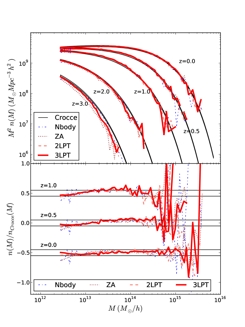
Figure 1: Mass function of the N-body simulation (thin blue dot-dashed lines) and pinocchio using the three LPT orders to construct haloes, at various redshifts: ZA (dotted brown lines), 2LPT (dashed pink lines) and 3LPT (thick red solid lines). The upper panel shows the quantity $M^{2}n(M)$ as a function of $M$, black thick lines give the (non-universal) analytic fit of Crocce et al. (2010). The lower panel shows the residuals with respect to the analytic fit for $z=0$, $0.5$ and $1$, conveniently displaced. The horizontal black lines give the $\pm 5$ per cent region around the Crocce fit.

2.3 Catalogue selection

In this paper we will test the accuracy of pinocchio in reproducing the results of N-body simulations run on the same initial conditions, both on a halo–by–halo basis and by checking the accuracy of the clustering statistics.

Catalogues for clustering analysis (based on the $1024^{3}$ setup) are defined as follows. From the full catalogues obtained, at $z=0$ and $z=1$, using both gadget and pinocchio, we define two sets of catalogues by selecting the haloes with at least 100 or 500 particles, corresponding to a selection of haloes more massive than $6.9\cdot 10^{12}M_{\odot}h^{-1}$ and $3.4\cdot 10^{13}M_{\odot}h^{-1}$, respectively. Before applying these cuts, the Warren correction (Warren et al., 2006) on the number of particles of FoF haloes is applied. These mass limits are set at the smallest FOF halo mass where we are fully confident that the reconstruction is correct and a larger mass where we still have sufficient statistics at $z=1$. We want to stress that the lower mass cut is motivated by the accuracy of N-body simulations, but pinocchio haloes, being built with a semi-analytic approach, are considered reliable as long as the mass function is well recovered.

3 Object by object comparison

A thorough investigation of the ability of pinocchio to recover FOF haloes from an N-body simulation run on the same seeds was presented in M02. In that paper halo matching was decided on the basis of the number of particles in common between N-body and pinocchio haloes. Our aim here is not to repeat the same detailed analysis (the main algorithm has not changed) but to assess how the increased LPT order impacts on group reconstruction. We then adopt a simpler and faster criterion for halo matching, and apply it to the smaller and more manageable $512^{3}$ simulation (see Section 2.1) at $z=0$.

For each halo produced by the pinocchio algorithm we consider the first particle that collapsed along the main progenitor branch, thus providing the earliest seed for the construction of the halo. Since it is likely to find this particle close to the bottom of the potential well of the N-body halo, if the corresponding particle in the N-body simulation belongs to a FOF halo then we match this pinocchio halo with the FOF one.

Considering each matched halo pair, the number of particles in common between the two haloes is recorded. Such number can be divided by the total number of particles of the pinocchio halo or of the FOF halo. Fig. 2 shows the distribution, for all matched halo pairs, of the fraction of common particles with respect to the pinocchio halo mass (upper panel) and with respect to the FOF halo mass (lower panel). Since the timing of the merging of two haloes into a bigger one may not be identical in pinocchio and in simulation, it can happen to match a halo before a merging with one after the corresponding merging, or vice versa. This, together with possible mis-matches due to numerics, justifies the tail to low values of these distributions. Loosely following M02, we define “cleanly matched” haloes the pairs that have both fractions above $30$ per cent. This relatively low value allows to obtain fraction of matched haloes in line with the detailed results of the 2002 paper. In Table 2 we report the number of cleanly matched haloes found in the different runs, where haloes are constructed with different LPT orders, as well as the total number of haloes in pinocchio catalogues and in simulations and the relative fractions. Overall, $\sim 70$ per cent of haloes are cleanly reconstructed, the number being dominated by the smallest masses where the reconstruction is less accurate.

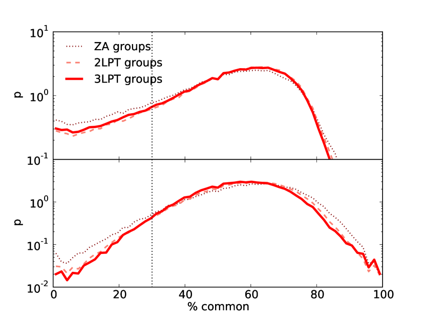
Figure 2: Distribution of the fraction of the particles that are in common between matched halo pairs, using different LPT orders in halo construction, as indicated in the label. The number of particles in common is normalized by the total number of particles of the pinocchio halo (top panel) or by the total number of particles of the FOF halo (bottom panel). In both panels, the distributions are normalized so that the integral of each one is unity. The vertical dotted line locates the threshold identifying the “clean” matched haloes.

Halo construction order	N CMH	N in pinocchio (% of CMH)	N in simulation (% of CMH)
ZA	134869	192819 (69.9%)	222118 (60.7%)
2LPT	146410	201019 (72.8%)	222118 (65.9%)
3LPT	144055	204687 (70.4%)	222118 (64.9%)

Table 2: Information on the statistics of cleanly matched haloes (CMH). In the first column the order with which haloes are constructed that identifies the catalogue used (independently of the displacement), in the second column the number of CMH, in the third column the total number of haloes in the full pinocchio catalogue and in parenthesis the percentage of the CMH, and in the fourth column the total number of haloes in the full FOF catalogue and in parenthesis the percentage of the CMH. Catalogues of haloes constructed with the same order of LPT but displaced with different orders of LPT provide the same number of matched haloes and are therefore not shown here.

In Fig. 3 the fraction of cleanly matched haloes (with respect to the total number of haloes in pinocchio catalogues) is shown as a function of FoF halo mass. In this plot we give results for haloes starting from 32 particles, to show the degradation taking place below the 100 particles limit. The higher order halo constructions (2LPT and 3LPT) perform better than ZA above $\sim 5\cdot 10^{12}M_{\odot}$, where resolution is good enough to reconstruct the haloes. The results for ZA are very similar with what was found in M02. It is worth stressing again that the fall of this fraction is not necessarily a sign of inaccuracy of pinocchio, but is surely due, at least in part, to the difficulty of recognising simulated haloes sampled by few particles.

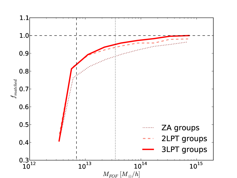
Figure 3: Fraction of cleanly matched haloes with respect to the total number of haloes in pinocchio catalogues as a function of FOF halo mass. Different colours refer to different runs where haloes are built via ZA, 2LPT or 3LPT (see legend). The vertical dashed line identifies the mass corresponding to 100 particles while the vertical dotted line locates the mass corresponding to 500 particles.

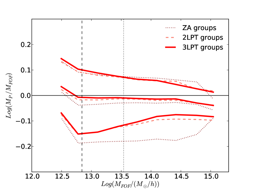
Figure 4: Relative accuracy of mass reconstruction for cleanly matched haloes as a function of the corresponding FOF mass, for halo constructed with different LPT orders, as indicated in the legend. For each order, the line in the middle is the median value, and the other two are the 16th and 84th percentiles. The vertical dashed and dotted lines mark the mass corresponding to 100 and 500 particles.

In Fig. 4 we show, for cleanly matched haloes, the log of the ratio of pinocchio and FOF masses as a function of FOF halo mass. Lines show the median and the 16th and 84th percentiles for groups reconstructed with ZA, 2LPT and 3LPT, as specified in the legend. It is apparent from this figure that the higher orders give better and more unbiased masses: typical accuracy in mass decreases form 0.18 dex for ZA to 0.13 dex for 2LPT and 3LPT, the highest order giving no obvious advantage. Moreover, the relative accuracy improves with mass. The negative bias visible at the largest masses is due to the fact that we are forcing two distributions of nearly equivalent objects to have the same mass function; if mass is recovered with some uncertainty at the object–to–object level, the mass functions can be equal only by introducing a negative bias in the reconstructed masses. We will get back to this point later.

Fig. 5 illustrates how well other halo properties are reconstructed by pinocchio. The panel on the top shows the median (and 16th and 84th percentiles) distance between cleanly matched halo pairs. These statistics are computed for bins of FOF halo mass, and shown as a function of this quantity. In this figure, that involves “Eulerian” quantities, we show six different models with halo construction and displacements performed with various LPT orders. The median distances are similar for the different configurations, except for the case of groups both constructed and displaced with ZA that presents a systematically larger value, although groups displaced with 3LPT present a smaller median distance in most of the explored range. The median distance in some runs has a mild positive dependence on halo mass, but the ratio of this distance with the halo Lagrangian radius is a decreasing function of halo mass, as discussed in Section 2.2.1.

The middle panel shows, with a very similar format, the difference in the modulus of velocity between matched halo pairs. This quantity has a mild dependence on mass, more massive haloes having a higher velocity difference. In this case, 3LPT gives an improvement over 2LPT only above $\sim 10^{14}M_{\odot}$, while below that value 2LPT gives a better reproduction of halo velocities. The panel at the bottom shows the distribution of the cosine of the angle between the velocities of the matched pairs. In all cases velocities are very well aligned (the median $\cos\theta$ being well below 0.95 in all cases), with the exception of a tail of less correlated velocities. ZA gives on average wider angles with a wider scatter around the median, indicating again a poorer reconstruction of halo properties.

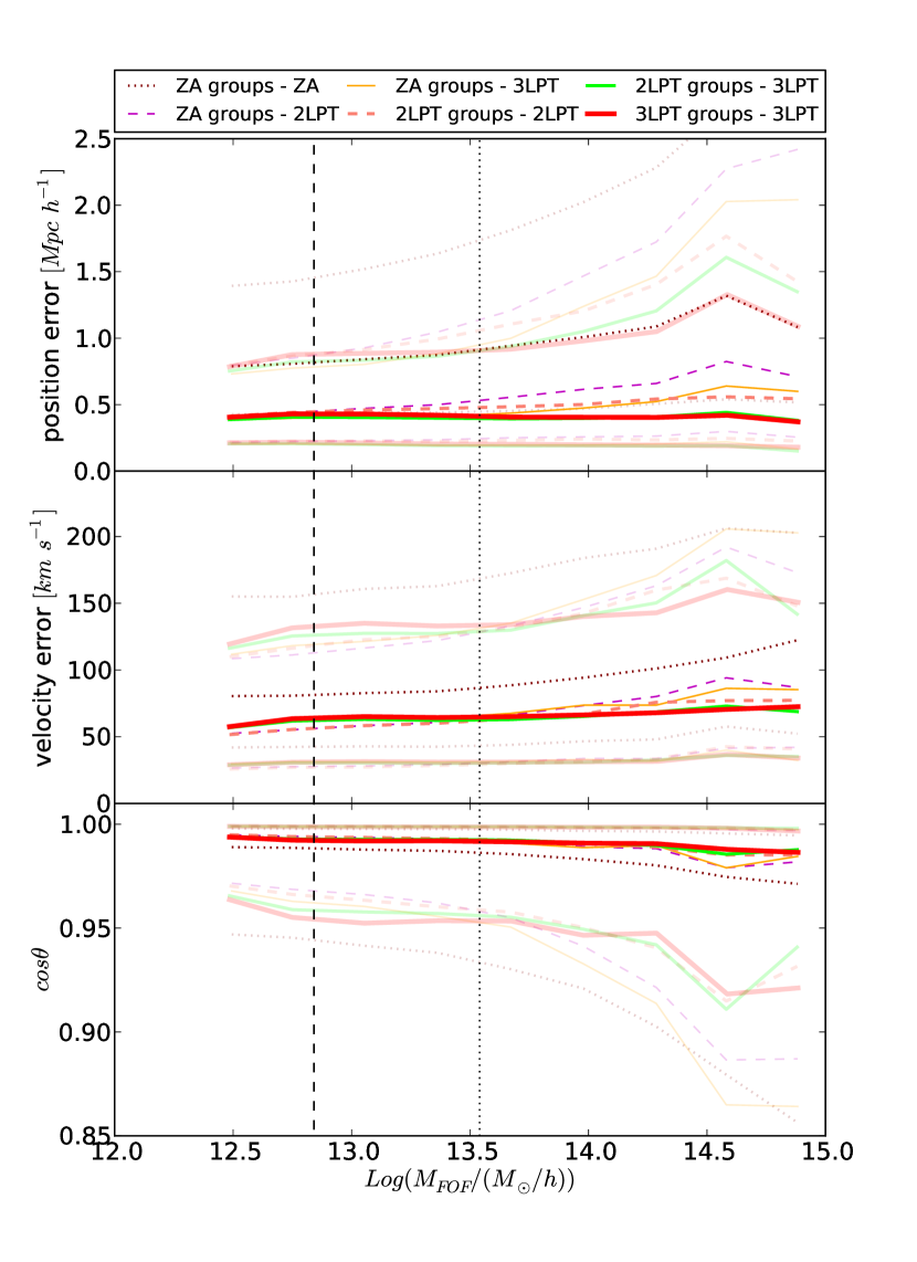
Figure 5: Position and velocity difference (top panel and middle panel, respectively) and cosine of the angle between velocity vectors (bottom panel) of pairs of cleanly matched haloes, for six combinations of LPT orders used for halo construction and halo displacement and velocity, as indicated in the legend. For each configuration shown, there are three lines, the one in the middle being the median, while the other two (shown in a pale shade) being the 16th and 84th percentiles. The vertical dashed and dotted lines identify the mass corresponding to 100 and 500 particles, respectively.

4 Clustering

In this section we make use of the catalogues described in Section 2.3, obtained with the setup of $1024^{3}$ particles in a 1024 Mpc/h box, and compute their clustering properties at $z=0$ and $1$. In the following, we will use $k_{MAX}=0.5\,{\rm h\,Mpc}^{-1}$ as reference frequency beyond which we expect non–linearities to become very important. It is worth stressing that the parameters of our code have already been calibrated by requiring a good fit of the simulated mass function, so clustering of haloes is a pure prediction of the code.

4.1 Power spectrum

There are two main sources of disagreement in the power spectra of pinocchio and simulations. On large scales, a difference in the linear bias term will give a constant offset, at small scales the power spectrum obtained with LPT displacements will drop below the simulated one beyond some wavenumber $k$. We decided to separate these two sources of disagreement, both to estimate in a more consistent way the $k$–value at which the power spectrum $P(k)$ drops below a certain level, and to stress that bias is a prediction of our code (see, e.g., Paranjape et al., 2013).

In Figure 6 we show the accuracy with which the power spectrum $P_{\rm sim}(k)$ of a FOF halo catalogue, in real space, is recovered by various versions of pinocchio that use increasing LPT orders for constructing and displacing haloes. The four groups of panels show results for the two mass cuts of 100 (upper panels) and 500 particles (lower panels), at $z=0$ (left panels) and $z=1$ (right panels). Each group of panels show in the upper stripe the recovery of the normalization of the power spectrum, quantified in this case as a linear bias term $b_{1}$, that is obtained as the square root of the average value of $P(k)$ divided by the matter power spectrum $P_{m}(k)$ of the simulation, computed over $k\leq 0.1\,{\rm h\,Mpc}^{-1}$:

$$P(k)=b_{1}^{2}\,P_{m}(k).$$ (4)

In the lower panels we show the ratio $P(k)/P_{\rm sim}(k)\times(b_{1,sim}/b_{1})^{2}$, i.e. the residuals of the pinocchio power spectrum with respect to the N-body one, normalized to unity for $k\leq 0.1{\rm h\,Mpc}^{-1}$. We will quantify the level of agreement between N-body and pinocchio power spectra as the wavenumber $k_{10\%}$ at which the normalized residuals go beyond a $[0.9,1.1]$ interval. We report in Table 3 the $k_{10\%}$ values for all the cases analysed below.

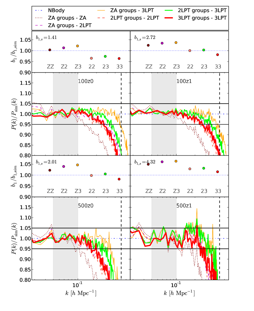
Figure 6: We show, for $z=0$ (left panels) and $z=1$ (right panels) and for the mass cuts of 100 (upper panels) and 500 particles (lower panels), the linear bias $b_{1}$, divided by the N–body’s one, and the power spectrum $P(k)$ in real space, divided by the one of FOF catalogue $P_{sim}$ and normalized to unity at $k\leq 0.1{\rm h\,Mpc}^{-1}$. The two black horizontal solid lines in the power spectrum panels locate the $10$ per cent accuracy region. The vertical dashed line locates $k_{MAX}$, while the shaded area locates the region of the BAO peak. In the bias panels we show the bias $b_{1}$ normalized by the one of the FOF catalogue from the simulation, the value of which is reported in each bias panel. The dotted blue horizontal line in the bias panels locates the value 1.

Considering haloes constructed with ZA and displaced with increasing LPT order (“ZZ”, “Z2”, “Z3”), we notice that, in terms of $k_{10\%}$, higher orders give a better recovery of the halo $P(k)$ at all redshifts and for all mass cuts: figures raise from $\sim 0.1-0.2$ to $\gtrsim 0.4-0.5\,{\rm h\,Mpc}^{-1}$, thus improving by at least a factor of two. The figure of $k_{10\%}=0.1{\rm h\,Mpc}^{-1}$ is consistent with the results of M13, while higher orders give negligible loss of power at the BAO scale. Regarding the bias, a clear trend of increasing $b_{1}$ with LPT order is visible; this time the “Z3” configuration is found to give the largest overestimate of $b_{1}$.

A different trend is found when 3LPT is used to displace the halos and the order for group reconstruction is varied (“Z3”, “23”, “33”). At $z=0$ $k_{10\%}$ decreases by a factor of two at $z=0$, while the effect is slightly less evident at $z=1$. Bias $b_{1}$ decreases with increasing LPT order, correcting for the overestimate given by the “Z3” configuration. Overall, the combination “Z3” of ZA groups and 3LPT displacements is the one that gives the best result in terms of $k_{10\%}$, but the combination “23” gives the best combination of power loss and bias. For this configuration $k_{10\%}$ is typically greater than $0.3\ {\rm h\,Mpc}^{-1}$, while bias $b_{1}$ is recovered at least to within 4 per cent in the worst case.

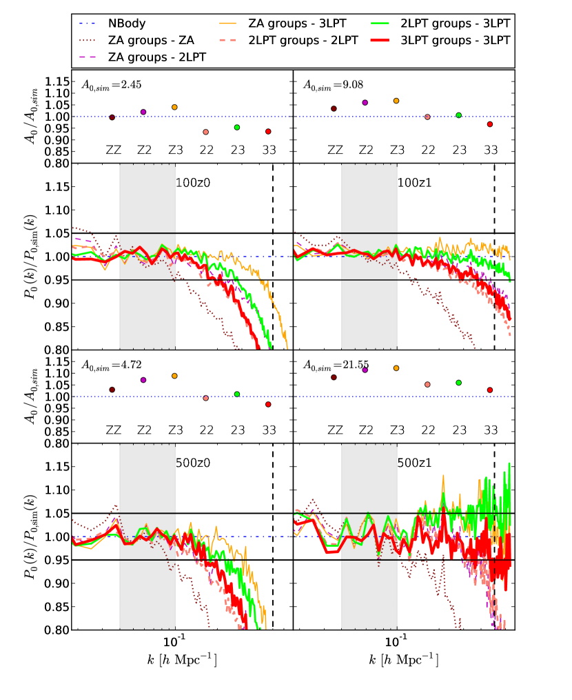
Figure 7: Recovery of the monopole $P_{0}(k)$ of the 2D power spectrum in redshift space. Panels and symbols are as in Figure 6. Upper rows give the measured value of the quantity $A_{0}$ as defined in equation 5.

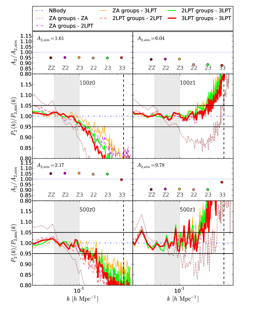
Figure 8: Recovery of the quadrupole $P_{2}(k)$ of the 2D power spectrum in redshift space. Panels and symbols are as in Figure 6. Upper rows give the measured value of the quantity $A_{2}$ as defined in equation 7.

Figure 7 shows the monopole $P_{0}(k)$ of the 2D power spectrum in redshift space. For this calculation we used the three axes as three lines of sight, and averaged the results over the three orientations. The monopole is related to the matter power spectrum via the following relation:

$$P_{0}(k)=A_{0}\,P_{m}(k),$$ (5)

where the coefficient $A_{0}$ in linear theory is equal to:

$$A_{0}=\left(1+\frac{2}{3}\beta+\frac{1}{5}\beta^{2}\right)b_{1}^{2},$$ (6)

where $\beta=f(\Omega_{m})/b_{1}$. The results are shown in the same format as in Figure 6. While the relative merits of the combinations of LPT orders are the same as in the real space $P(k)$, the ability to recover the mildly non-linear part of the power spectrum at $z=1$ is significantly better, with the best methods giving $k_{10\%}$ well in excess of $0.5{\rm h\,Mpc}^{-1}$. This advantage seems to be lost at $z=0$. Again, the combinations that perform better are those with groups displaced by 3LPT. The combination “Z3” is the best choice in terms of $k_{10\%}$, while “23” gives the best compromise between $k_{10\%}$ and $A_{0}$. When considering the high mass cut at $z=1$ the results are very noisy because of the poor statistics, but indicate that the “33” combination is the one that performs better. The accuracy in the recovery of the normalization $A_{0}$ is similar to that of $b_{1}$ once one takes into account that the coefficient depends on the square of bias. The best methods give agreement at the $5-10$ per cent level.

Fig. 8 shows the quadrupole $P_{2}(k)$ of the 2D power spectrum in redshift space, computed again as an average over the three axis orientations. The quadrupole is related to the matter power spectrum via the following relation:

$$P_{2}(k)=A_{2}\,P_{m}(k),$$ (7)

where the coefficient $A_{2}$ in linear theory is equal to:

$$A_{2}=\left(\frac{4}{3}\beta+\frac{4}{7}\beta^{2}\right)b_{1}^{2}.$$ (8)

In this case pinocchio catalogues show a strong power loss at $z=0$. At $z=1$ the tension is alleviated, the quadrupole appears compatible with the N–body’s one at low $k$, showing an excess of power for higher wavenumbers. For this specific observable, all the configurations, except “ZZ”, give comparable results, possibly due to the higher noise level that hides the fine details. In this case the “ZZ” configuration performs poorly even at the BAO scale, showing again the advantage of going to higher orders.

In linear regime, the growth rate $f$ is related to $\beta$ and to the bias $b_{1}$ via the following relation: $f=\beta\cdot b_{1}$. If we multiply the mean value of $b_{1}$ within $k=0.1{\rm h\,Mpc}^{-1}$ with $\beta$, obtained by solving the ratio given by eq. 5 divided by eq. 7 and averaged in the same range of $b_{1}$, we obtain values of the growth rate that are consistent with the actual theoretical value $f\simeq\Omega_{m}^{0.6}$.

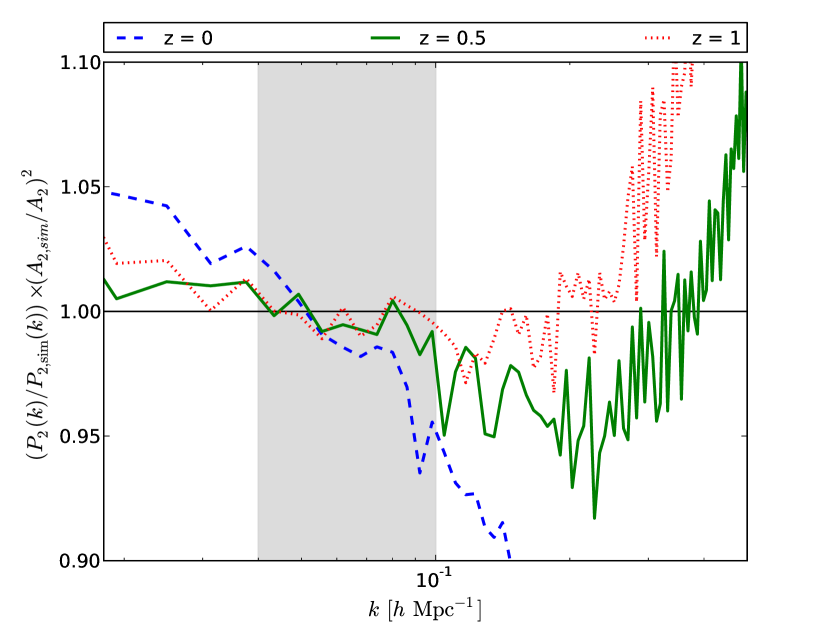
Figure 9: Recovery of the quadrupole for the configuration “22” for the catalogue “100” at three different redshifts, as indicated in the legend. The shaded area locates the region of the BAO peak.

To further investigate the degradation of the agreement in the quadrupole term at low redshift, in Figure 9 we show the recovery of the quadrupole for the configuration “22” and only for the catalogue “100” at three different redshifts, namely 0, 0.5 and 1. This configuration allows a direct comparison with what was found in Chuang et al. (2015a), as in that paper the redshift was $0.56$, the number density $3.5\times 10^{-4}{\rm h^{3}Mpc}^{-3}$, and pinocchio was run with 2LPT both for halo construction and displacement (the number density of our “100” catalogue at $z=0.5$ is $3.85\cdot 10^{-4}$). The behaviour of the quadrupole at $z=0.5$ is compatible with that found in Chuang et al. (2015a), with a loss of power that reaches a minimum of $\sim 8$ per cent at $k\simeq 0.2{\rm h\,Mpc}^{-1}$, and a successive gain of power that allows the quadrupole to reach the N–body’s value at $k\simeq 0.4{\rm h\,Mpc}^{-1}$. What is evident from Figure 9 is the evolution of the quadrupole with redshift. For redshift above 0.5, that is very relevant for future surveys, the quadrupole is within $10$ per cent accuracy for $k\lesssim 0.3{\rm h\,Mpc}^{-1}$.

	100 z0	100 z1	500 z0	500 z1
Power spectrum real space
ZA groups - ZA	0.21	0.23	0.15	0.21
ZA groups - 2LPT	0.39	0.38	0.24	0.29
ZA groups - 3LPT	0.55	0.54	0.38	0.42
2LPT groups - 2LPT	0.31	0.36	0.22	0.33
2LPT groups - 3LPT	0.43	0.47	0.34	0.44
3LPT groups - 3LPT	0.34	0.37	0.25	0.37
Monopole redshift space
ZA groups - ZA	0.16	0.21	0.13	0.21
ZA groups - 2LPT	0.34	0.61	0.23	0.45
ZA groups - 3LPT	0.50	0.64	0.38	0.64
2LPT groups - 2LPT	0.28	0.51	0.20	0.49
2LPT groups - 3LPT	0.35	0.64	0.31	0.64
3LPT groups - 3LPT	0.28	0.58	0.23	0.64
Quadrupole redshift space
ZA groups - ZA	0.09	0.54	0.09	0.63
ZA groups - 2LPT	0.25	0.36	0.18	0.29
ZA groups - 3LPT	0.30	0.36	0.58	0.29
2LPT groups - 2LPT	0.14	0.37	0.18	0.29
2LPT groups - 3LPT	0.17	0.35	0.28	0.25
3LPT groups - 3LPT	0.15	0.45	0.21	0.29

Table 3: $k_{10\%}$ values, in units of $\rm h\,Mpc^{-1}$, beyond which the normalized residuals of the pinocchio power spectra with respect to the N-body ones differ by more than $10$ per cent from unity.

Given these results, in the following clustering analysis we focus our attention only on the configurations that perform better in the power spectrum analysis, that is haloes constructed with ZA and displaced with 3LPT (“Z3”) and haloes constructed with 2LPT and displaced with 3LPT (“23”). We will also consider the “22” configuration, that has significant smaller memory requirements, and, for comparison with previous work, the “ZZ” configuration of the previous version of pinocchio, with haloes constructed and displaced with ZA.

4.2 Bispectrum

The distribution of DM haloes is characterised by a high level of non-Gaussianity resulting from both the nonlinear evolution of matter perturbation as from the nonlinear and non-local properties of halo bias (see e.g. Chan et al., 2012). In particular such non-Gaussianity is responsible for relevant contributions to the covariance of the galaxy power spectrum (see, e.g. Hamilton et al., 2006; de Putter et al., 2012) and it is therefore crucial that any approximate method aiming at reproducing halo clustering can properly account for it.

Non-Gaussianity is simply defined by the non-vanishing of any (or all) connected correlation function of order higher than the two point function (for a generic introduction see Bernardeau et al., 2002). Here we simply consider the lowest order in the correlation function hierarchy, limiting ourselves to a comparison of bispectrum $B(k_{1},k_{2},k_{3})$, i.e. the 3-PCF in Fourier space. As opposed to sampling a few subsets of triangular configurations (as done for instance in M13), here we attempt a comparison between all measurable configurations defined by triplets of wavenumber $(k_{1},k_{2},k_{3})$ up to $0.2\,{\rm h/Mpc}$. Specifically we consider wavenumber values defined by linear bins of size 3 times the fundamental frequency of the box.

The top panels of Fig. 10 show the distribution obtained from individual values of the relative difference $[B(k_{1},k_{2},k_{3})-B_{sim}(k_{1},k_{2},k_{3})]/B_{sim}(k_{1},k_{2},k_{3})$ evaluated for all triangular configurations $k_{1},k_{2},k_{3}$ with $0.2\,{\rm h/Mpc}\geq k_{1}\geq k_{2}\geq k_{3}$. It is evident that higher-order LPT, when compared to ZA results based on ZA displacements, reduces the variance of such distribution at $z=0$. The differences between the other redshifts and the other orders is, on the other hand, less evident, but in three out of four panels “Z3” is found to overestimate the relative difference, while “23” gives less biased results.

The lower panel shows a similar comparison this time for the reduced bispectrum $Q(k_{1},k_{2},k_{3})$ defined as the ratio $Q(k_{1},k_{2},k_{3})=B(k_{1},k_{2},k_{3})/P(k_{1})P(k_{2})+perm$. This quantity has the advantage of highlighting the dependence on the triangle shape by reducing the overall dependence on scale, particularly significant in the penuchi result due to the lack of power at small scales. In fact, we notice that pinocchio predictions are slightly more accurate for the reduced bispectrum than for the bispectrum itself.

The results confirm what was found in M13, that the ability of the code to recover clustering extends to higher order statistics, and show improvements with respect to the original version based on ZA both for group construction and displacement.

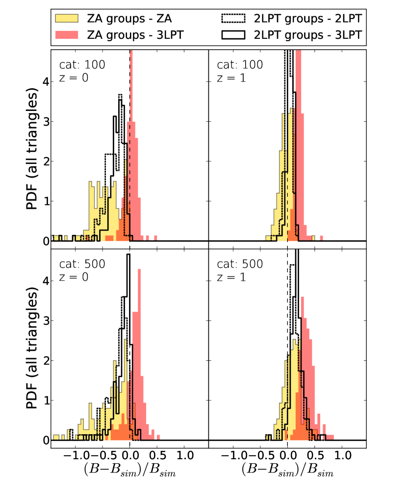
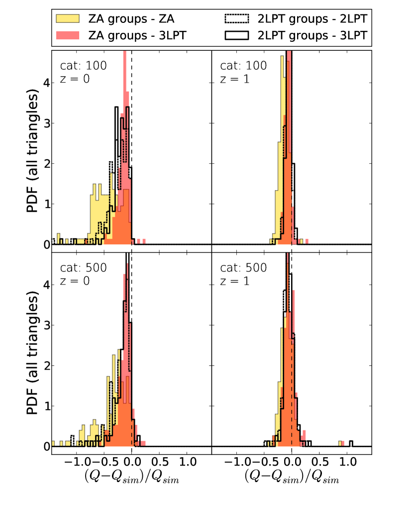
Figure 10: Pdf of the relative difference of the bispectrum (top panels) and reduced bispectrum (bottom panels) with respect to the N–body’s ones for four configurations, as indicated in the legend. The four subpanels refer to $z=0$ and $1$ (left and right columns, respectively) and high and low mass cuts (top and bottom rows, respectively), as indicated in the figures. All the triangles up to $k=0.2{\rm h\,Mpc}^{-1}$ are considered.

4.3 Phase correlations

The phase difference between the halo field in pinocchio and in the simulation could give an indication of how important stochasticity, i.e. coupling between long and short wavelenght fluctuations, is and how much of it is not captured by our Lagrangian schemes for the displacements (Seljak & Warren, 2004). In this respect the LPT order used to construct groups plays a minor role. Fig. 11 shows the phase difference between the FOF catalogue from simulation and the pinocchio catalogues built according to different criteria for the halo construction and for the halo displacements. For each catalogue we have computed the density field of haloes by adopting a CIC (count in cell) algorithm on a $150^{3}$ cell grid. After Fourier transforming the density field, the angles between the k–vectors in the simulation and in each pinocchio catalogue are computed.

For all the pinocchio runs, the median is compatible with 0, with comparable scatters around it, except for the catalogue built with ZA for both the construction and the displacements, that presents a wider scatter. As expected, the phase difference is symmetrc around zero, a direct consequence of the density field being a real field.

The good recovery of the phase information, or stochasticity, in the halo density field comes naturally from the good performance of the pinocchio on a object by object basis. This also makes pinocchio best suitable for cross correlation between different tracers of the dark matter density field, as opposed to other methods based on sampling, which are tuned to reproduce auto power spectra only.

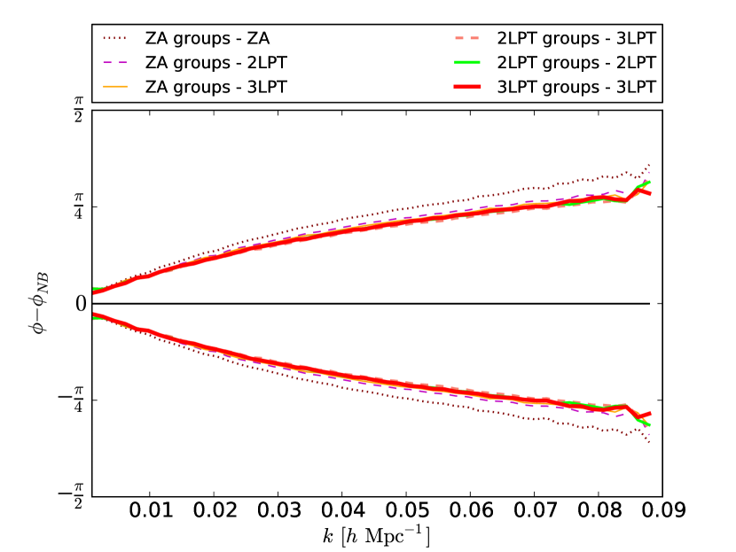
Figure 11: Phase difference, computed on a $150^{3}$ cell grid at $z=0$, between the FOF catalogue from simulation and the pinocchio catalogues built according to different criteria for the halo construction and for the halo displacements as indicated in the legend. The median values in each k–bin for each run are plotted as black solid lines that overlap one another, while the 16 and 84 percentiles are coded as reported in the legend.

4.4 2–point correlation function

Figures 12 to 14 show the 2-point correlation function in real and redshift space (monopole and quadrupole). Following Manera et al. (2010), here we rescale the correlation functions in the [30-70] $h^{-1}$ Mpc interval to match the large scale bias, as done in Sect. 4.1 for the power spectrum. The correlation function, both in real and in redshift space, is well reproduced by the different configurations, being within $10$ per cent of the N–body’s one for most of the explored radial range, with the obvious exception of the zero-crossing region (where the correlation function reaches the value 0, at $~{}120-140h^{-1}\rm Mpc$) and of the first radial bin, where the clustering is underestimated. While runs with groups constructed with ZA appear to have little or no bias, runs with groups constructed with higher LPT orders present a $5-10\%$ bias. Besides that, differences between runs are small so that it is hard to decide which choice is best; the comparison in Fourier space gives a much clearer view of the differences.

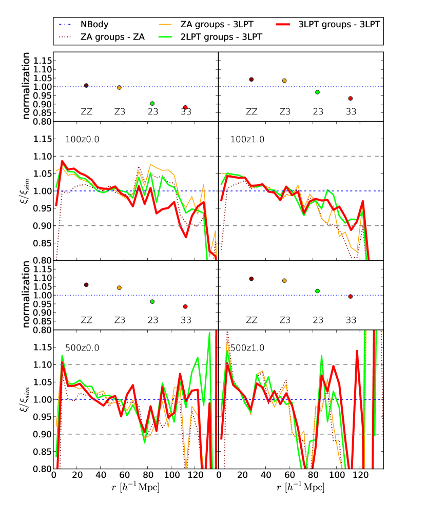
Figure 12: 2–point correlation function in real space. For the high (top panels) and low mass cut catalogues (bottom panels), at redshift 0 (left columns) and 1 (right columns), we show, in the lower subpanels, the ratio of the 2–point correlation function with respect to the N–body’s one, normalized by the mean value in the [30-70] $h^{-1}$ Mpc interval, and the values of such normalization in the upper subpanels. The configurations shown are those indicated in the legend.

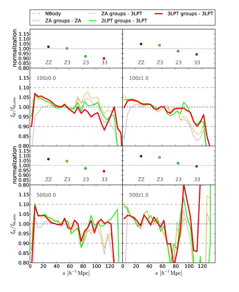
Figure 13: Same as 13 but for the monopole in redshift space.

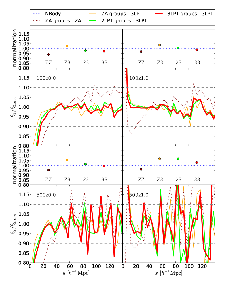
Figure 14: Same as 13 but for the quadrupole in redshift space.

4.5 The origin of inaccuracy in the recovery of the linear bias term

pinocchio is able to recover halo masses with a good accuracy, as shown in Figure 4, where the average mass is in good agreement with the one from simulation. However, the recovery is subject to scatter of $\sim 0.15$ dex. At the same time, the mass function is fit to within a 5-10 per cent accuracy. Because most of the recovered haloes are closely matched, an unbiased mass recovery would lead to an overestimate of the mass function, and this justify the little underestimate in the average mass visible in that figure, especially at large masses (where the mass function is steeper and then more subject to this effect). When applying mass cuts, different haloes will be selected and, given the steepness of the mass function, it is more likely that a halo is up–scattered to higher values of mass rather than it is down–scattered to smaller values. This will induce an underestimate in the halo bias measured for the sample, that could justify some of the differences found in our previous analysis.

We have quantified this effect as follows. We have perturbed the masses of the FoF catalogue from simulation with a log-normal distribution with zero mean and dispersion as found in Figure 4 for the ZA case. Then we have applied the usual mass cuts of 100 and 500 particles. Figure 15 shows the ratio of the power spectra $P(k)$ in real space of the perturbed catalogues and the original ones. Clearly, this time the residuals are not normalized to unity on large scales, and the insets give the mean of the plotted ratios. The perturbed catalogues present a relative (squared) bias of $\sim 3-5$ per cent at $z=0$, and of $5-6$ per cent at $z=1$. The error in the recovery of bias that we have quantified above are larger than these numbers, so this effect can justify only part of the discrepancies that we find.

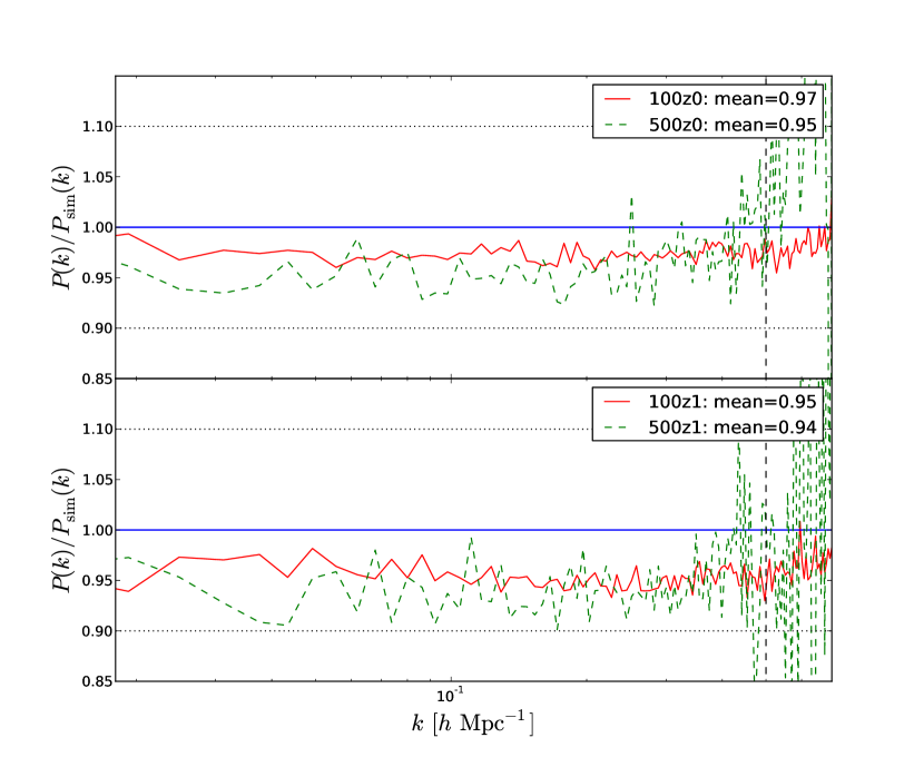
Figure 15: Ratio between the power spectrum of the perturbed FOF catalogues and the unperturbed one. Solid red lines refer to the high number density catalogues, while green dashed lines refer to the low density ones. The horizontal blue line locates the value 1, while the horizontal dotted ones locate the $10$ per cent accuracy region. The vertical dashed line locates $k_{MAX}$. The top panel shows the results at $z=0$, while the bottom panel at $z=1$. In the legend the mean values of the ratios, computed for the values below $k=0.3{\rm h\,Mpc}^{-1}$, are reported.

We now demonstrate that the inaccuracy in the recovery of bias is driven by mismatches in halo recovery. To this aim we use the setup with $512^{3}$ particles, taking advantage of the object-by-object match performed in Section 3, and we consider the mass cut corresponding to 100 particles at $z=0$. We first restrict the catalogue to cleanly matched halo pairs, so that we have the same number of objects in the two catalogues and no difference can be ascribed to the effect described above. We compute the power spectrum in real space at $z=0$ for these sets of haloes, and we repeat the procedure for all combinations of LPT order. It is worth stressing that the N-body catalogues in this case are different for each group construction, as matching depends on how haloes are constructed. In the left panel of Figure 16 we show the ratios of $P(k)$ of pinocchio and N-body catalogues; again, ratios here are not normalized to unity at large scales. The bias in the power spectrum of the cleanly matched haloes is recovered to within a few per cent, especially when higher orders are used: haloes displaced with 3LPT are within 1 per cent of the power spectrum of the simulation within $k=0.2{\rm h\,Mpc}^{-1}$, meaning that $b_{1}$ is accurate by 0.5 per cent.

Conversely, the right panel of Figure 16 shows the ratios of power spectra of pinocchio and FoF haloes (not normalized to unity at large scales) for the whole catalogue, including mismatched halos. The ratios range from 0.93 to 1.07, consistent with the bias values found above, and are comparable but larger than the effect quantified in Figure 15. The bias is therefore strongly affected by mismatches in halo reconstruction. Here reconstruction with ZA, that is the least accurate at the object-by-object level, leads to a 7% boost that is present even at $k\sim 0.4\ {\rm h\,Mpc}^{-1}$.

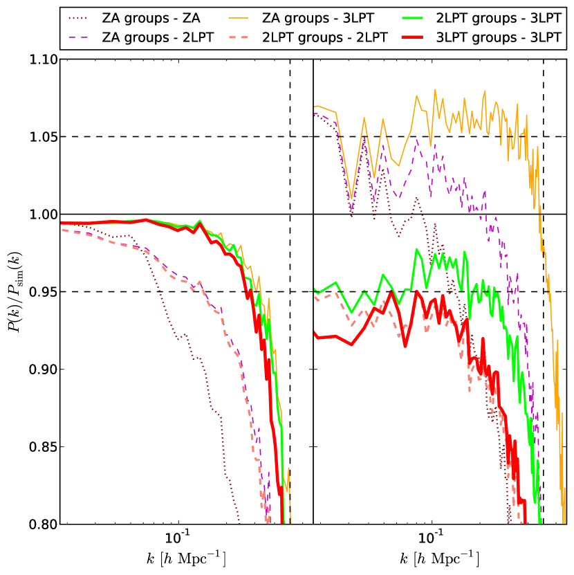
Figure 16: Comparison between the power spectrum in real space at $z=0$ of the catalogue made only by matched haloes in the $512^{3}$ particle – 512 Mpc/h side box setup (left panel) and that with all haloes (right panel), namely the catalogue “100” described in Sect. 2.3. Power spectra are normalized by the power spectra extracted from the corresponding catalogues of the N–body simulation. The horizontal solid line marks the value 1, while the horizontal dashed one located the $10$ per cent accuracy limit. The vertical dashed line locates $k_{MAX}$. In the legend, alongside the name of each configuration we report the mean value of the power spectrum within $k=0.1{\rm h\,Mpc}^{-1}$, the first value being relative to the matched haloes catalogues and the second one to the “100” catalogue.

5 Conclusions

We have tested the latest version of the pinocchio code, with displacements computed up to the third order of LPT. We have compared the results of an N-body simulation with those obtained by running our code on the same initial configuration, so that the agreement extends to the object–by–object level. We have then quantified the advantage of going to higher LPT orders, making a distinction between halo construction and displacement at catalogue output.

The main results are the following.

• The mass function is used as a constraint to calibrate parameters that regulate accretion and merging. This calibration is performed so as to reproduce the mass function of FoF haloes to within a few per cent, and is cosmology independent, so it is performed once for all. Halo clustering is entirely a prediction of the code.

• We have compared pinocchio and simulated haloes at the object–by–object level. The construction of the haloes, in terms of number of particles, does not depend strongly on the order used for the halo construction, although with ZA shows a poorer level of agreement. with respect to the N–body’s one. For cleanly matched objects, increasing the displacement order leads to halo positions and velocities closer to those of the corresponding halo in the N–body simulation.

• We have computed the power spectrum in real space and the monopole and quadrupole of the 2D power spectrum in redshift space of catalogues produced with increasing LPT orders for halo construction and displacement, comparing them to those of the N–body simulation. Catalogues are constructed to have the same mass cuts (100 and 500 particles), and two redshifts ($z=0$ and $1$). We have quantified separately the accuracy with which the normalization is recovered on large scales, as a linear bias term $b_{1}$ for real space and constants $A_{0}$ and $A_{2}$ for redshift space, and the wavenumber $k_{10\%}$ at which discrepancies in the power spectrum amount to $10$ per cent.

• Higher LPT orders give significant improvements to the accuracy of halo clustering. 3LPT generally provides the best agreement with N–body when it is used to displace haloes, while lower LPT orders are better when used for halo construction. Linear bias is typically recovered at the few per cent level when higher orders for the displacements are used, while $k_{10\%}$ is found in the range from 0.3 to 0.5, if not higher. The quadrupole is recovered to a similar level of accuracy at $z=1$, but suffers significant degradation between $z=0.5$ and $z=0$.

• Good agreement is confirmed by an analysis of the bispectrum, where again higher orders give improved accuracy. The improvement of higher LPT orders is confirmed by an analysis of phase correlations.

• The 2–point correlation function is well reproduced within $10$ per cent in most of the explored radial range, although runs with haloes constructed with higher LPT orders present a $5-10\%$ bias.

• We have investigated the reason for the few per cent discrepancy in the recovery of linear bias. Part of it ($\sim 2-3$ per cent) is due to the scatter in the reconstructed halo masses, coupled with the selection criterion, and a comparable amount ($\sim 3-4$ per cent) is due to mismatches in halo definition between pinocchio and FoF.

These results confirm, from the one hand, the validity of the pinocchio code in predicting the clustering of DM haloes to a few per cent level and on scales that are not deeply affected by non-linearities. On the other hand, it shows that higher LPT orders give a definite advantage in this sense, and that they provide predictions that are accurate enough, even in the era of high-precision cosmology, for applications like the construction of covariance matrices. We conclude that, though 2LPT provides already a good improvement with respect to ZA and though 3LPT almost doubles memory requirements, the latter can be considered as a very good choice for displacing the haloes. From another point of view, collapse times are computed by solving the collapse of a homogeneous ellipsoid using 3LPT; it must be stressed that 3LPT in this context is different from the one used to compute displacements (that contain a much higher degree of non-locality, while ellipsoidal collapse depends entirely on the Hessian of the peculiar potential), but consistency in the LPT order is welcome. Moreover, 3LPT is the lowest LPT order that allows to compute consistently in perturbation theory the four-point correlation function, that determines the covariance of two-point statistics, one of the most obvious applications of an approximate code like pinocchio.

We have also considered separately the effect of 3LPT in constructing haloes and in displacing them. The highest order provides noticeably advantages at displacing haloes, while for halo constructions lower orders perform better. Though the best results in term of $k_{10\%}$ are obtained with the “Z3” combination, where halos are constructed with Zel’dovich approximation and displaced with 3LPT, we recommend “23” as the best option, because it gives the best combination of bias and power loss at small scales, besides a less biased bispectrum, and because the gain in power of “Z3” is due to mismatched halos (Figure 16). Indeed, the ZA gives the worst performance at the object-by-object level, and the worst mass function at high redshift.

The loss of accuracy at higher LPT order in this case is not completely unexpected. Halo construction is based on an extrapolation of LPT to the orbit crossing point, that is to the point when the perturbation approach breaks, and then its validity degrades with a higher level of non linearity. In this context, higher order terms are not guaranteed to give an improvement. Conversely, halo displacement at catalogue output implies an average over the whole halo, that is an average over the whole region that goes into orbit crossing. In a forthcoming paper (Munari et al., in preparation), we will investigate how several approximate methods to displace particles are able to reproduce the clustering of haloes, starting from the knowledge of the particles that belong to the haloes in the simulation. A result that we anticipate is that 3LPT is not able to concentrate halo particles into a limited, high-density region, but it is able to displace the haloes with very good accuracy, once positions are averaged over the multi-stream region. This confirms that 3LPT may not be optimal for reconstructing haloes, but it is very effective in placing their centre of mass into the right position.

Appendix A Implementation and performance

With respect to v3.0, presented in M13, pinocchio v4.0 has been completely re-written in C, and re-designed to achieve an optimal use of memory. These are the main improvements.

(1) LPT displacements are computed as follows (e.g. Catelan, 1995):

$$\vec{x}(t)=\vec{q}+D(t)\vec{S}^{(1)}(\vec{q})+D_{2}(t)\vec{S}^{(2)}(\vec{q})+$$

$$+D_{3a}(t)\vec{S}^{(3a)}(\vec{q})+D_{3b}(t)\vec{S}^{(3b)}(\vec{q})$$

where $\vec{q}$ and $\vec{x}$ are the Lagrangian and Eulerian coordinates, respectively, and the $D_{i}$ and $\vec{S}^{i}$ terms are the factorized time and space parts of the LPT terms. The $S^{i}$ terms can be expressed as gradients of a potential, the 3c rotational term is typically very small and is neglected here. The equations for these terms are reported in Catelan (1995). To be able to compute the displacement of a particle at a generic time $t$, it is then necessary to store four vectors for each particle. Consistently with the original algorithms, the spatial parts are computed at the same smoothing scale at which the particle is predicted to collapse; we have verified that results are very similar if this assumption is dropped and displacements are computed on the unsmoothed density field. As discussed in the main text, different orders for displacements can be applied at halo construction and catalogue output. Memory requirements amount to $80$ bytes per particle for ZA, $145$ for 2LPT and $250$ for 3LPT, with slightly higher figures to allow for the memory overhead described in point (2) below. As for the computing time, higher orders require more memory and will then be distributed on a higher number of MPI tasks; we have noticed that the computing time increases less rapidly than memory requirement, so higher order do typically require slightly less elapsed time to be performed.

(2) The second part of the code, the fragmentation of collapsed medium into haloes, is parallelized by dividing the simulation volume into sub-volumes, and fragmenting the sub-volumes without any further communication. To avoid border effects, a boundary layer must be taken into account in order to correctly construct haloes near the border. The width of this layer is scaled according to the Lagrangian size of the largest object expected to be present in the simulated volume. This size can be rather large at $z=0$, amounting to $\sim 30$ Mpc. This means that relatively small volumes at high resolution might require a significant memory overhead due to these boundary layers, especially if the computation is distributed over many cores. To limit this problem, fragmentation is performed by dividing the volume in a few slabs and distributing those over tasks, thus performing the fragmentation in steps. This further sub-division of the simulation volume decreases the memory requirement for each sub-volume while increasing the overhead (being the size of the boundary layer fixed), but it gives in general an advantage, allowing in most cases to perform the fragmentation.

(3) Displacements are now computed on the unsmoothed density field. In previous versions, particle displacements were computed at the same smoothing radius at which the particle collapses. But in fact halo displacements are obtained by averaging over halo particles, and this is in itself a sort of smoothing, that would cumulate with the previous one. Moreover, computing LPT displacements several times for several smoothing radii gives a significant overhead, that can be avoided. As a matter of fact, differences between the two schemes (computing displacements at each smoothing or only for the unsmoothed field) are minor.

(4) An algorithm has been devised to output a catalogue of haloes on the past light cone. As a starting point, the position of a halo can be easily computed at any time as long as its mass does not change. Then, each time halo mass is updated, a check is performed on whether the halo has crossed the light cone since last time it was checked. This check is repeated for a set of periodic replications of the box that cover the required survey geometry. This algorithm therefore provides a continuous reconstruction of the past light cone, without resorting to a finite number of snapshots. The reconstruction of the past light cone will be tested in a future paper.

(5) With respect to the naive implementation of M13, the redistribution of memory from the plane-based scheme of the first part of the code to the sub-volume-based scheme of the second part is done using a hypecubic communication scheme. Being this very efficient, communications are subdominant in any configuration.

Figure 17 gives strong and weak scaling tests for the new version of the code, obtained (analogously to M13) by distributing a volume of 1.2 Gpc/h sampled by $900^{3}$ particles on a number of cores ranging from $16$ to $14\times 16=224$ (strong scaling), and running a set of boxes, at the same mass resolution, from $900^{3}$ to $2160^{3}$ particles (weak scaling). In this test we used 2LPT displacements for haloes building and catalogues, and we gave enough memory so that fragmentation does not require the box to be divided into slices (see point (2) above). We show the total CPU time (in hours) needed by several parts of the code. An ideal scaling, constant for the strong test and growing like $N\log N$ for the weak test, is given by the black continuous line. Because, thanks to the FFTW package, (Frigo & Johnson, 2012), FFTs scale very closely to the ideal case, and because the rest of the code performs distributed computations and i/o is kept to a minimum, the scaling is very close to ideal for the strong test and better than ideal for the weak test.

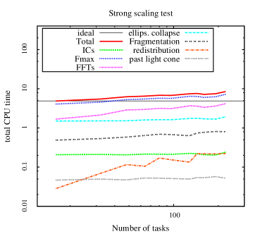
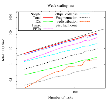
Figure 17: Strong (left) and weak (right) scaling tests for the code, in the configuration specified in the main text. The various lines give the computing time required by various parts of the code, as specified in the legend: initial conditions (the initial density field), “Fmax” (the computation of inverse collapse times for all smoothing radii), FFTs, the computation of ellipsoidal collapse, fragmentation (or halo construction), redistribution of memory from planes to sub-volumes, past-light-cone construction. The black continuous line gives ideal scaling, i.e. a constant time for the weak test and $N\log N$ for the strong test.

As a matter of fact, the FFT solver gives the strongest limitation to the largest run that is feasible with this code. This is due to the fact that memory is distributed in planes, so a task must have memory for at least one plane. A mixed MPI-OpenMP configuration helps in making this limitation less stringent: a plane is loaded onto an MPI task that accesses more memory, the computation is distributed over many threads using OpenMP. We have implemented this configuration and verified that its scaling is worse than the pure MPI case. We are currently working to overtake this limit by using an FFT solver that distributes memory with a more flexible geometry (in pencils or cubes).

To understand whether the results presented in the paper depend on resolution, for the same configuration used throughout the paper we have run pinocchio using $512^{3}$ and $2048^{3}$ particles. The generation of random seeds allows to have the same large-scale structure when the number of particles per side is increased or decreased by factors of two. In this test we use 2LPT for both halo construction and displacement. From these runs, catalogues have been extracted with mass cuts of 100 and 500 particles, as explained in Section 2.3. The reference catalogue is that cut at 500 particles, in order to have a good sampling even in the lower resolution run. In Fig. 18 the power spectrum in real space is shown in the upper panel, while the lower panel gives the residuals with respect to the N-body power spectrum. When comparing the standard run with the lower resolution one, pinocchio catalogues show some dependence on resolution, but the high resolution run shows that convergence is reached at our standard resolution.

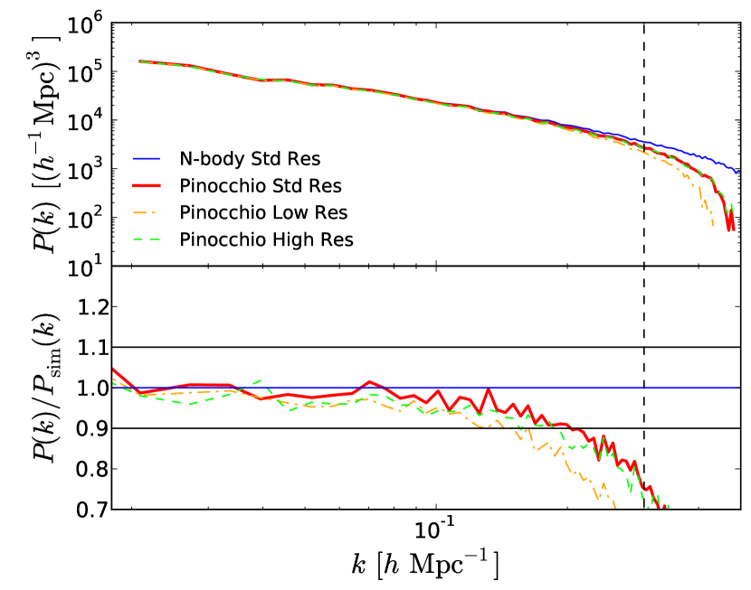
Figure 18: Power spectrum in real space (top panel) for different runs, both for N–body simulation and for pinocchio, as indicated in the legend: “Std” refers to the $1024^{3}$ particle runs, “Low Res” to the $512^{3}$ particle runs and “High Res” to the run with $2048^{3}$ particles and same box size. All the runs are made with 2LPT both for the halo construction and displacement. In the bottom panel we show the ratio of the power spectra with that of the standard resolution N–body run. The horizontal blue line gives unity value, while the horizontal dotted ones give the $\pm 10$ per cent accuracy region. The vertical dashed line gives $k_{MAX}$.

Appendix B Calibration

Name	Box size	N.	Particle Mass	N.
	(Mpc/h)	particles	(M${}_{\odot}/h$)	realizations
VeLar	$4096.0$	$1024^{3}$	$4.44\cdot 10^{12}$	10
Large	$2048.0$	$1024^{3}$	$5.55\cdot 10^{11}$	10
Mediu	$1024.0$	$1024^{3}$	$6.93\cdot 10^{10}$	10
Small	$512.0$	$1024^{3}$	$8.67\cdot 10^{9}$	10
VeSma	$256.0$	$1024^{3}$	$1.08\cdot 10^{9}$	10

Table 4: Main properties of the five sets of runs used for the calibration.

To calibrate pinocchio against an analytical, universal mass function, we produced five sets of runs using $1024^{3}$ particles and box sizes from $4096$ to $256$ Mpc$/h$ (Table 4). Particle masses thus range from $1.08\cdot 10^{9}$ to $4.44\cdot 10^{12}$ M${}_{\odot}/h$, a factor of $\sim 4000$ in variation. This allows to reliably sample the mass function on almost five orders of magnitude in mass. For each set we produced runs with 10 different random seeds, to beat down sample variance. The Mediu boxes are analgous to the $1024^{3}$ setup of the paper, the first one being exactly the same run.

To better visualize the violation of universality versus the level of non-linearity $D\sigma$, we consider the rescaled mass function $f(\nu)$ produced by pinocchio at some redshift $z$, corresponding to a given $D\sigma$: $f(\nu,D\sigma)$. We take for each set of runs the average over the ten realizations. We then take the ratio of this quantity with an analytic, universal mass function; we consider here the fit proposed by Watson et al. (2013). Then we consider four small intervals of $\nu$ around four specific values, with semi-amplitude of 0.2, and compute the average value of $f(\nu,D\sigma)/f_{\rm watson}(\nu)$ in the bin. This is a set of functions of $D\sigma$, one for each set of runs and each $\nu$ value. The upper panel of Figure 20 shows these functions for 3LPT displacements and a choice of parameters $f=0.501$, $e=0.745$, while $s_{a}=s_{e}=0$.

The functions show a clear maximum at $D\sigma\sim 1.2$. We take this as the value of the $D\sigma_{0}$ parameter. Results change very slowly with $D\sigma_{0}$, and small variations are degenerate with $s_{a}$ and $s_{m}$, so there is no need to fine-tune this parameter. At lower values, pinocchio mass functions show a modest systematic underestimate with respect to Watson. We noticed a similar behaviour with simulations, so we interpret this as a sign that mass resolution is not sufficient to properly reproduce haloes and do not attempt to correct for it. On the other hand, the decrease at $D\sigma>D\sigma_{0}$, that is not seen in the N-body case (where the curves grow due to the violation of universality), is interpreted as the effect of increasing inaccuracy of displacements. The lower panels show the effect of using optimal values of $s_{a}=0.334$ and $s_{m}=0.052$ to improve the fit.

Best-fit parameters were found by running the code on a grid of parameter values, studying the effect of their variations on the mass function at some relevant $\nu$ and $D\sigma$ values, finding the degeneracies between parameters, and then guessing a value that minimizes the differences. Figure 19 shows the final calibrated mass function. As in Figure 1, the upper panel shows $M^{2}n(M)$ for the five sets of runs, together with the Watson analytic mass function, while the lower panels show the residuals. We will show below that the steepening of some mass functions at low $z$ is within the uncertainty of the numerical mass function. In principle one could recalibrate the code for any analytic mass function. At fixed $D\sigma$, some very small variations with resolution, at the few percent level, are present in the figures. They grow to $\sim 10$ percent at the lowest resolution VeLar. To fix it one could introduce an explicit dependence on resolution (through $\sigma$ in place of $D\sigma$) but the mass resolution of VeLar is so poor that we do not foresee any application of it.

The high tail of the mass function ($\nu\geq 3$) tends to overestimate the Watson fit at late times, with some dependency on resolution. In figure 21 we show the bunch of $f(\nu)$ curves versus several analytic formulas, including Sheth & Tormen (2002), Crocce et al. (2010), Tinker et al. (2008), Courtin et al. (2011) and Angulo et al. (2012). At $\nu\sim 3-4$ mass functions predicted by pinocchio show a spread, filling the region from the Watson and Angulo fits to the Crocce and Courtin one. This trend grows with time, and is stronger at lower resolution (higher $D\sigma$). The likely origin of this trend is the following. The separation of merging and accretion naturally depends on mass resolution, as a particle that accretes on a halo will possibly contain haloes at a lower resolution. We are fixing the growing inaccuracy of displacements by increasing merging and accretion in a separate way, through constant $s_{a}$ and $s_{m}$ parameters. A more sophisticated approach should take into account the resolution-dependent separation of accretion and merging. Because the results are within the uncertainty of the numerical mass function, we do not attempt to implement this sophistication now.

Analogous calibrations have been performed for ZA and 2LPT. Best-fit parameters are given in Table 5. All these parameters give a universal mass function. In this context, non-universality can be easily obtained (as in the main text to follow the trend of the N-body simulation) at a given resolution but, because the main dependency is with $D\sigma$, the redshift evolution of this non-universality will depend on resolution.

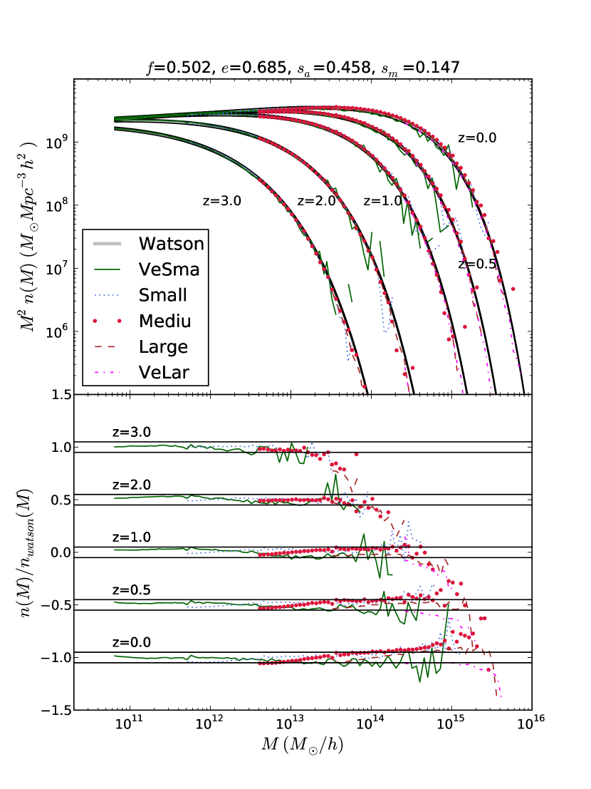
Figure 19: Mass function produced for the five sets of runs, compared with the Watson et al., 2013 fit. The upper panel shows the quantity $M^{2}n(M)$ as a function of $M$ The lower panel shows the residuals with respect to the analytic fit, conveniently displaced. The horizontal black lines give the $\pm 5$ per cent region.

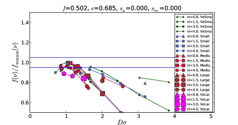
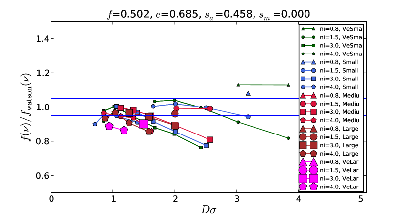
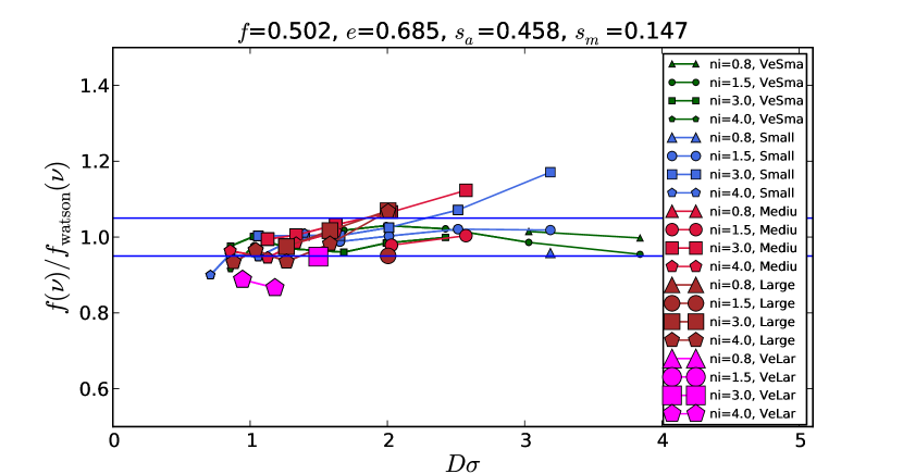
Figure 20:

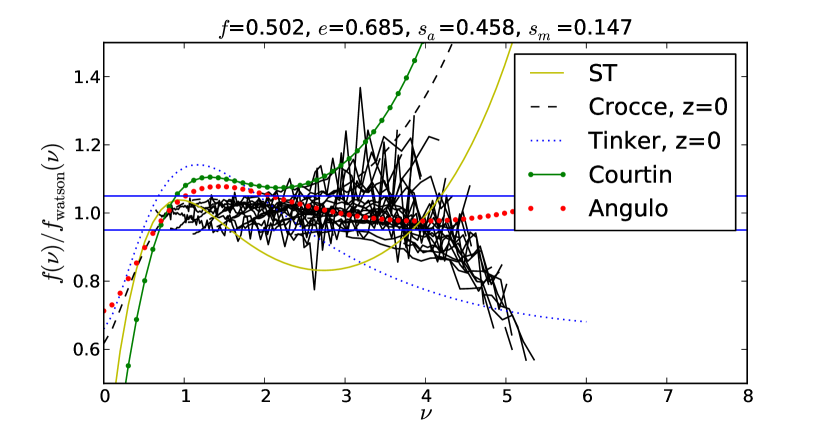
Figure 21: Rescaled mass function $f(\nu)$, divided by the Watson et al., 2013 fit, for all the runs (black lines) performed with 2LPT and for the best-fit parameters. Colored curves give other numerical fits, as illustrated in the legend (see references in the text).

Parameter	ZA value	2LPT value	3LPT value
$f$	0.505	0.501	0.502
$e$	0.820	0.745	0.685
$s_{a}$	0.300	0.334	0.458
$s_{m}$	0.000	0.052	0.148
$D\sigma_{0}$	1.7	1.5	1.2

Table 5: Adopted values of the parameters of eq. 3 for the calibration of the mass function against the Watson et al., 2013 analytical fit.

References

- Angulo et al. (2012) Angulo R. E., Springel V., White S. D. M., Jenkins A., Baugh C. M., Frenk C. S., 2012, MNRAS, 426, 2046
- Avila et al. (2015) Avila S., Murray S. G., Knebe A., Power C., Robotham A. S. G., Garcia-Bellido J., 2015, MNRAS, 450, 1856
- Bernardeau et al. (2002) Bernardeau F., Colombi S., Gaztañaga E., Scoccimarro R., 2002, Phys. Rep., 367, 1
- Borgani et al. (1995) Borgani S., Plionis M., Coles P., Moscardini L., 1995, MNRAS, 277, 1191
- Catelan (1995) Catelan P., 1995, MNRAS, 276, 115
- Chan et al. (2012) Chan K. C., Scoccimarro R., Sheth R. K., 2012, Phys. Rev. D, 85, 083509
- Chuang et al. (2015a) Chuang C.-H., Kitaura F.-S., Prada F., Zhao C., Yepes G., 2015a, MNRAS, 446, 2621
- Chuang et al. (2015b) Chuang C.-H., et al., 2015b, MNRAS, 452, 686
- Coles et al. (1993) Coles P., Melott A. L., Shandarin S. F., 1993, MNRAS, 260, 765
- Courtin et al. (2011) Courtin J., Rasera Y., Alimi J.-M., Corasaniti P.-S., Boucher V., Füzfa A., 2011, MNRAS, 410, 1911
- Crocce et al. (2010) Crocce M., Fosalba P., Castander F. J., Gaztañaga E., 2010, MNRAS, 403, 1353
- Despali et al. (2015) Despali G., Giocoli C., Angulo R. E., Tormen G., Sheth R. K., Baso G., Moscardini L., 2015, preprint, (arXiv:1507.05627)
- Feng et al. (2016) Feng Y., Chu M.-Y., Seljak U., 2016, preprint, (arXiv:1603.00476)
- Frieman & Dark Energy Survey Collaboration (2013) Frieman J., Dark Energy Survey Collaboration 2013, in American Astronomical Society Meeting Abstracts 221. p. 335.01
- Frigo & Johnson (2012) Frigo M., Johnson S. G., 2012, FFTW: Fastest Fourier Transform in the West, Astrophysics Source Code Library (ascl:1201.015)
- Green et al. (2012) Green J., et al., 2012, preprint, (arXiv:1208.4012)
- Hamilton et al. (2006) Hamilton A. J. S., Rimes C. D., Scoccimarro R., 2006, MNRAS, 371, 1188
- Hartlap et al. (2007) Hartlap J., Simon P., Schneider P., 2007, A&A, 464, 399
- Howlett et al. (2015) Howlett C., Manera M., Percival W. J., 2015, Astronomy and Computing, 12, 109
- Izard et al. (2015) Izard A., Crocce M., Fosalba P., 2015, preprint, (arXiv:1509.04685)
- Kitaura et al. (2014) Kitaura F.-S., Yepes G., Prada F., 2014, MNRAS, 439, L21
- Kitaura et al. (2015) Kitaura F.-S., Gil-Marín H., Scóccola C. G., Chuang C.-H., Müller V., Yepes G., Prada F., 2015, MNRAS, 450, 1836
- Koda et al. (2015) Koda J., Blake C., Beutler F., Kazin E., Marin F., 2015, preprint, (arXiv:1507.05329)
- LSST Science Collaboration et al. (2009) LSST Science Collaboration et al., 2009, preprint, (arXiv:0912.0201)
- Laureijs et al. (2011) Laureijs R., et al., 2011, preprint, (arXiv:1110.3193)
- Levi et al. (2013) Levi M., et al., 2013, preprint, (arXiv:1308.0847)
- Manera et al. (2010) Manera M., Sheth R. K., Scoccimarro R., 2010, MNRAS, 402, 589
- Manera et al. (2013) Manera M., et al., 2013, MNRAS, 428, 1036
- Manera et al. (2015) Manera M., et al., 2015, MNRAS, 447, 437
- Mohammed & Seljak (2014) Mohammed I., Seljak U., 2014, MNRAS, 445, 3382
- Monaco (1995) Monaco P., 1995, ApJ, 447, 23
- Monaco (1997) Monaco P., 1997, MNRAS, 287, 753
- Monaco et al. (2002) Monaco P., Theuns T., Taffoni G., 2002, MNRAS, 331, 587
- Monaco et al. (2013) Monaco P., Sefusatti E., Borgani S., Crocce M., Fosalba P., Sheth R. K., Theuns T., 2013, MNRAS, 433, 2389
- Niklas Grieb et al. (2015) Niklas Grieb J., Sánchez A., Salazar-Albornoz S., dalla Vecchia C., 2015, preprint, (arXiv:1509.04293)
- O’Connell et al. (2015) O’Connell R., Eisenstein D., Vargas M., Ho S., Padmanabhan N., 2015, preprint, (arXiv:1510.01740)
- Paranjape et al. (2013) Paranjape A., Sefusatti E., Chan K. C., Desjacques V., Monaco P., Sheth R. K., 2013, MNRAS, 436, 449
- Paz & Sánchez (2015) Paz D. J., Sánchez A. G., 2015, MNRAS, 454, 4326
- Percival et al. (2014) Percival W. J., et al., 2014, MNRAS, 439, 2531
- Pope & Szapudi (2008) Pope A. C., Szapudi I., 2008, MNRAS, 389, 766
- Schlegel et al. (2011) Schlegel D., et al., 2011, preprint, (arXiv:1106.1706)
- Scoccimarro & Sheth (2002) Scoccimarro R., Sheth R. K., 2002, MNRAS, 329, 629
- Seljak & Warren (2004) Seljak U., Warren M. S., 2004, MNRAS, 355, 129
- Sheth & Tormen (2002) Sheth R. K., Tormen G., 2002, MNRAS, 329, 61
- Springel (2005) Springel V., 2005, MNRAS, 364, 1105
- Sunayama et al. (2015) Sunayama T., Padmanabhan N., Heitmann K., Habib S., Rangel E., 2015, preprint, (arXiv:1510.06665)
- Taffoni et al. (2002) Taffoni G., Monaco P., Theuns T., 2002, MNRAS, 333, 623
- Tassev et al. (2013) Tassev S., Zaldarriaga M., Eisenstein D. J., 2013, J. Cosmology Astropart. Phys., 6, 36
- Tassev et al. (2015) Tassev S., Eisenstein D. J., Wandelt B. D., Zaldarriaga M., 2015, preprint, (arXiv:1502.07751)
- Tinker et al. (2008) Tinker J., Kravtsov A. V., Klypin A., Abazajian K., Warren M., Yepes G., Gottlöber S., Holz D. E., 2008, ApJ, 688, 709
- Warren et al. (2006) Warren M. S., Abazajian K., Holz D. E., Teodoro L., 2006, ApJ, 646, 881
- Watson et al. (2013) Watson W. A., Iliev I. T., D’Aloisio A., Knebe A., Shapiro P. R., Yepes G., 2013, MNRAS, 433, 1230
- White et al. (2014) White M., Tinker J. L., McBride C. K., 2014, MNRAS, 437, 2594
- de Putter et al. (2012) de Putter R., Wagner C., Mena O., Verde L., Percival W. J., 2012, J. Cosmology Astropart. Phys., 4, 019