Ionization fraction and the enhanced sulfur chemistry in Barnard 1

Abstract

Context. Barnard B1b has been revealed as one of the most interesting globules from the chemical and dynamical point of view. It presents a rich molecular chemistry characterized by large abundances of deuterated and complex molecules. Furthermore, this globule hosts an extremely young Class 0 object and one candidate for the first hydrostatic core (FHSC) proving the youth of this star-forming region.

Aims. Our aim is to determine the cosmic ray ionization rate, $\zeta_{H_{2}}$, and the depletion factors in this extremely young star-forming region. These parameters determine the dynamical evolution of the core.

Methods. We carried out a spectral survey toward Barnard 1b as part of the IRAM large program $``$IRAM Chemical survey of sun-like star-forming regions$"$ (ASAI) using the IRAM 30-m telescope at Pico Veleta (Spain). This provided a very complete inventory of neutral and ionic C-, N-, and S- bearing species with, from our knowledge, the first secure detections of the deuterated ions DCS⁺ and DOCO⁺. We use a state-of-the-art pseudo-time-dependent gas-phase chemical model that includes the ortho and para forms of H₂, H${}_{2}^{+}$, D${}_{2}^{+}$, H${}_{3}^{+}$, H₂D⁺, D₂H⁺, D₂, and D${}_{3}^{+}$ to determine the local value of the cosmic ray ionization rate and the depletion factors.

Results. Our model assumes n(H₂)=10⁵ cm^-3 and T_k=12 K, as derived from our previous works. The observational data are well fitted with $\zeta_{H_{2}}$ between 3$\times$10^-17 s^-1 and 10^-16 s^-1 and the elemental abundances O/H=3 10^-5, N/H=6.4$-$8 10^-5, C/H=1.7 10^-5, and S/H between 6.0 10^-7 and 1.0 10^-6. The large number of neutral/protonated species detected allows us to derive the elemental abundances and cosmic ray ionization rate simultaneously. Elemental depletions are estimated to be $\sim$10 for C and O, $\sim$1 for N, and $\sim$25 for S.

Conclusions. Barnard B1b presents similar depletions of C and O as those measured in prestellar cores. The depletion of sulfur is higher than that of C and O, but not as extreme as in cold cores. In fact, it is similar to the values found in some bipolar outflows, hot cores, and photon-dominated regions. Several scenarios are discussed to account for these peculiar abundances. We propose that it is the consequence of the initial conditions (important outflows and enhanced UV fields in the surroundings) and a rapid collapse ($\sim$0.1 Myr) that allows most S- and N-bearing species to remain in the gas phase to great optical depths. The interaction of the compact outflow associated with B1b-S with the surrounding material could enhance the abundances of S-bearing molecules, as well.

1 Introduction

Cosmic rays (hereafter CRs) play a leading role in the chemistry, heating, and dynamics of the interstellar medium (ISM). By ionizing their main component, molecular hydrogen, CRs interact with dense molecular clouds, and this process initiates a series of ion-molecule reactions that form compounds of increasing complexity to eventually build up the rich chemistry observed in dark clouds (see, e.g., Wakelam et al., 2010). Also, CRs represent an important heating source for molecular clouds. Collisions with interstellar molecules and atoms convert about half of the energy of primary and secondary electrons yielded by the ionization process into heat (Glassgold & Langer, 1973; Glassgold et al., 2012). Finally, the ionization fraction controls the coupling of magnetic fields with the gas, driving the dissipation of turbulence and angular momentum transfer, thus playing a crucial role in protostellar collapse and the dynamics of accretion disks (see Padovani et al., 2013 and references therein).

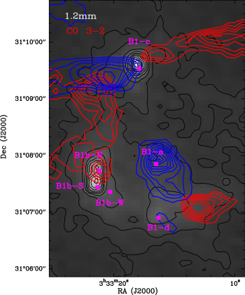
Figure 1: Continuum map at 1.2 mm observed at the IRAM telescope with the MAMBO instrument (Daniel et al., 2013). The contours are 20mJy/beam, 40 mJy/beam to 400 mJy/beam in steps of by 40 mJy/beam. Contours show the high velocity blue (2.5 to 4.5 km s^-1) and red (8.5 to 11.5 km s^-1) emission of the CO 3$\rightarrow$2 line as observed with the JCMT (project S12AC01).

The cosmic ray ionization rate $\zeta_{H_{2}}$ is the number of hydrogen molecule ionization per second produced by CRs. In absence of other ionization agents (X-rays, UV photons, J-type shocks), the ionization fraction is proportional to $\sqrt{\zeta_{H_{2}}}$, which becomes the key parameter in the molecular cloud evolution (McKee, 1989; Caselli et al., 2002). During the last 50 years, values of $\zeta_{H_{2}}$ ranging from a few 10^-18 s^-1 to a few 10^-16 s^-1 have been observationally determined in diffuse and dense interstellar clouds (Galli & Padovani 2015, and references therein). The cosmic ray ionization rate has usually been estimated from the [HCO⁺]/[CO] and/or [DCO⁺]/[HCO⁺] abundance ratios using simple analytical expressions (e.g., Guelin et al., 1977; Wootten et al., 1979; Dalgarno & Lepp, 1984). In recent studies, these estimates have been improved using comprehensive chemistry models (Caselli et al., 1999; Bergin et al., 1999). These models show that the gas ionization fraction is also dependent on the depletion factors that should be known to accurately estimate $\zeta_{H_{2}}$ (Caselli et al., 1999).

Chemical modeling is required to constrain the elemental abundances and the cosmic ray ionization rate. We carried out a spectral survey toward Barnard 1b as part of the IRAM large program $``$IRAM Chemical survey of sun-like star-forming regions$"$ (ASAI) (PIs: Rafael Bachiller, Bertrand Lefloch) using the IRAM 30-m telescope at Pico Veleta (Spain), which provided a very complete inventory of ionic species including C-, N-, and S-bearing compounds. The large number of neutral/protonated species allows us to derive the elemental abundances in the gas phase and cosmic ray ionization rate simultaneously, avoiding the uncertainty due to unknown depletion factors in the latter.

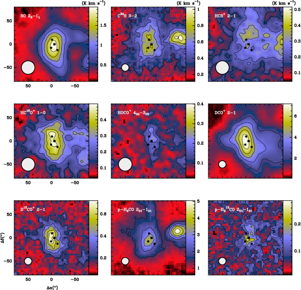
Figure 2: Integrated intensity maps of the SO 2₂$\rightarrow$1₁, C³⁴S 3$\rightarrow$2, HCS⁺ 2$\rightarrow$1, HC¹⁸O⁺ 1$\rightarrow$0, HOCO⁺ 4₀₄$\rightarrow$3₀₃, DCO⁺ 2$\rightarrow$1, D¹³CO⁺ 2$\rightarrow$1, p-H₂CO 2₀₂$\rightarrow$2₀₁, and p-H₂¹³CO 2₀₂$\rightarrow$2₀₁ lines. The HPBW of the 30-m telescope at each line frequency is drawn in the bottom-left corner of the panel. The stars indicate the positions of B1b-N, B1b-S and B1b-W. The black square shows the position targeted in the unbiased spectral survey.

Barnard 1 (B1) belongs to the Perseus molecular cloud complex (D=235 pc). The Barnard 1 dark cloud itself is subdivided into several dense cores at different evolutionary stages of star formation. While B1-a and B1-c are known to host class 0 sources associated with high velocity outflows (Hatchell et al., 2005, 2007), the B1-b core appears to be more quiet, although its western edge is interacting with an outflow that is possibly arising from sources B1-a or B1-d, which are both located 1$\arcmin$ SW of B1-b (see a sketch in Fig. 1).

The B1b region was mapped in many molecular tracers, for example, HCO⁺, CS, NH₃, ¹³CO (Bachiller & Cernicharo, 1984; Bachiller et al., 1990), N₂H⁺ (Huang & Hirano, 2013), H¹³CO⁺ (Hirano et al., 1999), or CH₃OH (Hiramatsu et al., 2010; Öberg et al., 2010). Interferometric observations of Barnard 1b revealed that this compact core hosts two young stellar objects (YSOs), B1b-N and B1b-S (Huang & Hirano, 2013), and a third more evolved source, hereafter B1b-W, with deep absorption from ices (Jørgensen et al., 2006). The two first sources are deeply embedded in the surrounding protostellar envelope, which seems essentially unaffected by the embedded sources as shown by the large column density, N(H₂)$\sim$7.6$\times$10²² cm^-2 (Daniel et al., 2013), and cold kinetic temperature, T_K = 12 K (Lis et al., 2010). Based on Herschel fluxes and subsequent SED modeling, Pezzuto et al. (2012) concluded that B1b-N and B1b-S were younger than Class 0 sources and proposed these as first hydrostatic core (FHSC) candidates. Using NOEMA, Gerin et al. (2015) obtained high resolution maps of the protostellar ouflows and their envelope, confirming the young ages of B1b-N and B1b-S ($\sim$1000 yr and $\sim$3000 yr) and the high density of the surrounding core ($\sim$ a few 10⁵ cm^-3 for the outflowing gas).

From the chemical point of view, B1b is characterized by a rich chemistry. Indeed, many molecules were observed for the first time in this object, like HCNO (Marcelino et al., 2009) or CH₃O (Cernicharo et al., 2012). Additionally, B1b shows a high degree of deuterium fractionation and has been associated with first detections of multiply deuterated molecules, such as ND₃ (Lis et al., 2002) or D₂CS (Marcelino et al., 2005), which is consistent with the expected chemistry in a dense and cold core.

Table 1: Observing and telescope parameters.

Freq (GHz)	$\Delta$v (km s-1)	HPBW1	$B_{eff}$	rms(Ta) (mK)
82.5$-$117.6	0.1255	29$\arcsec$$-$21$\arcsec$	0.81$-$0.78	3$-$52
130.0$-$172.7	0.3424	19$\arcsec$$-$14$\arcsec$	0.74	6$-$103
200.6$-$275.9	0.2839	12$\arcsec$$-$9$\arcsec$	0.63$-$0.49	5$-$10

¹HPBW(arcsec)$\approx$2460/Freq(GHz); ²rms$\sim$240 mK for $\nu$$>$114 GHz,; ³rms$\sim$500 mK for $\nu$$>$169 GHz.

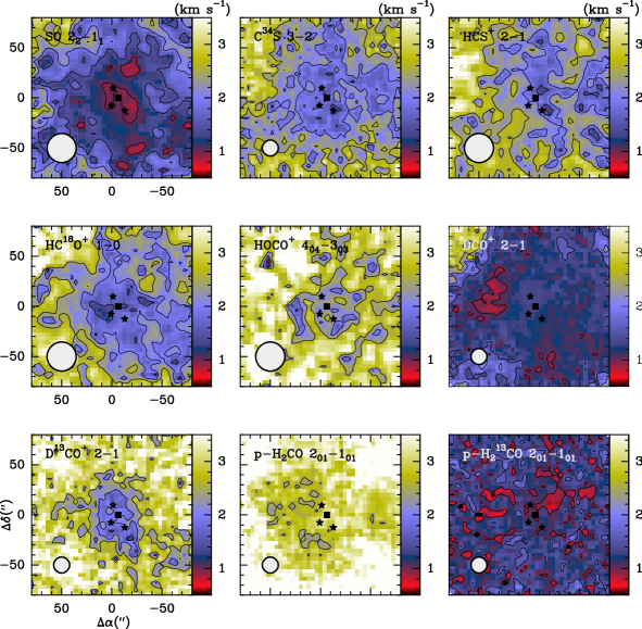
Figure 3: Maps of the linewidths of the SO 2₂$\rightarrow$1₁, C³⁴S 3$\rightarrow$2, HCS⁺ 2$\rightarrow$1, HC¹⁸O⁺ 1$\rightarrow$0, HOCO⁺ 4₀₄$\rightarrow$3₀₃, DCO⁺ 2$\rightarrow$1, D¹³CO⁺ 2$\rightarrow$1, p-H₂CO 2₀₂$\rightarrow$2₀₁, p-H₂¹³CO 2₀₂$\rightarrow$2₀₁ lines. Symbols are the same as in Fig. 2.

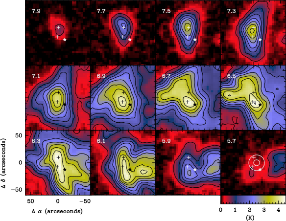
Figure 4: Spectral maps of the DCO⁺ 2$\rightarrow$1 line as observed with the IRAM 30-m telescope. The central velocity is indicated in the top-left corner. Contours are 0.5 K to 4.5 K by steps of 0.5 K. The crosses indicate the positions of the protostellar cores B1b-N and B1b-S. The star denotes the position of B1b-W. In the last panel we plot the beam at 144.277 GHz.

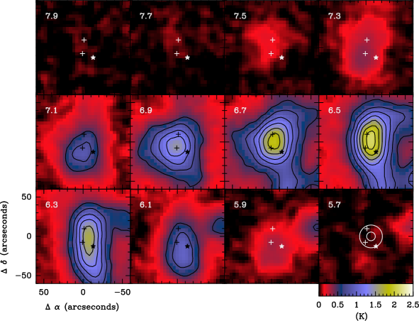
Figure 5: Spectral maps of the SO 2₂$\rightarrow$1₁ line as observed with the IRAM 30-m telescope. The central velocity is indicated in the top-left corner. Contours are 0.5 K to 4.5 K by steps of 0.25 K. The crosses indicate the positions of the protostellar cores B1b-N and B1b-S.The star denotes the position of B1b-W. In the last panel we plot the beam at 86.094 GHz.

2 Observations

We carried out a spectral survey toward Barnard B1b ($\alpha_{\rm J2000}$=03$\mathrm{h}$ 33 $\mathrm{m}$ 20.8 $\mathrm{s}$,  $\delta_{\rm J2000}$=31^∘ 07’ 34”.0) using the IRAM 30-m telescope at Pico Veleta (Spain). This position is in between the two FHSC candidates B1b-N and B1b-S. The two protostellar cores lie inside the HPBW of the 30-m telescope at 3 mm, but they are missed at 1 mm wavelengths (see Fig. 2).

The 3 mm observations were performed between January and May 2012 (see Cernicharo et al., 2012), which used the narrow mode of the FTS allowing a higher spectral resolution of 50 kHz. The observing mode in this case was frequency switching with a frequency throw of 7.14 MHz, which removes standing waves between the secondary and the receivers. Several observing periods were scheduled on July and February 2013 and January and March 2014 to cover the 1 and 2 mm bands shown in Table 1. The Eight MIxer Receivers (EMIR) and the Fast Fourier Transform Spectrometers (FTS) with a spectral resolution of 200 kHz were used for these observations. The observing procedure was wobbler switching with a throw of 200$\arcsec$ to ensure flat baselines. In Table 1 we show the half power beam width (HPBW), spectral resolution, and sensitivity achieved in each observed frequency band. The whole dataset will be published elsewhere but this paper is centered on the ionic species and sulfur compounds.

We complemented the unbiased spectral survey with 175$\arcsec$$\times$175$\arcsec$ maps of the SO 2₂$\rightarrow$1₁, C³⁴S 3$\rightarrow$2, HCS⁺ 2$\rightarrow$1, HC¹⁸O⁺ 1$\rightarrow$0, HOCO⁺ 4₀₄$\rightarrow$3₀₃, DCO⁺ 2$\rightarrow$1, D¹³CO⁺ 2$\rightarrow$1, p-H₂CO 2₀₂$\rightarrow$2₀₁, p-H₂¹³CO 2₀₂$\rightarrow$2₀₁ lines (see Fig. 2). These maps were simultaneously observed at 3 and 2 mm with a combination of the EMIR receivers and the Fourier transform spectrometers, which yields a bandwidth of 1.8 GHz per sideband per polarization at a channel spacing of 49 kHz. The tuned frequencies were 85.55 and 144.90 GHz. We used the on-the-fly scanning strategy with a dump time of 0.5 seconds and a scanning speed of 10.9$\arcsec$/s to ensure a sampling of at least three dumps per beam at the 17.8$\arcsec$ resolution of the 2 mm lines. The 175$\arcsec$$\times$175$\arcsec$ region was covered using successive orthogonal scans along the RA and DEC axes. The separation between two successive rasters was 6.5$\arcsec$ ($\sim$ $\lambda$/2D) to ensure Nyquist sampling at the highest observed frequency, i.e., 145 GHz. A common reference position located at offsets (200$\arcsec$, 150$\arcsec$) was observed for 10 seconds every 77.5 seconds. The typical IRAM 30 m position accuracy is 3$\arcsec$.

The data reduction and line identification were carried out with the package GILDAS/CLASS software.

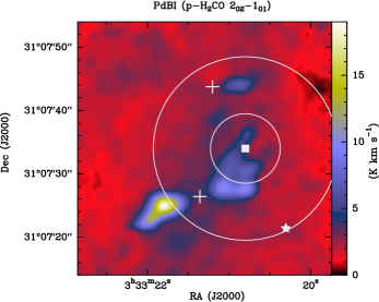
Figure 6: Interferometric integrated intensity map of the outflows associated with B1b-N and B1b-S in the H₂CO 2_0,2$-$1_0,1 line (Gerin et al., 2015). The crosses indicate the positions of the protostellar cores, B1b-N and B1b-S, and the star, of B1b-W. The position targeted by our spectral survey is drawn with a white square and the beams of the 30-m telescope at 3nmm and 1mm are indicated by white circles.

3 Methodology

Our goal is to use the database provided by the IRAM large program ASAI together with previous millimeter data from our group (Marcelino et al., 2005, 2009, 2010; Cernicharo et al., 2012, 2013; Daniel et al., 2013; Cernicharo et al., 2014; Gerin et al., 2015) and complementary mapping to accurately determine the fundamental chemical parameters.

Within our spectral survey we detected the following ions: HCO⁺, H¹³CO⁺, HC¹⁸O⁺, HC¹⁷O⁺, DCO⁺, D¹³CO⁺, HOCO⁺, DOCO⁺, HCS⁺, SO⁺, HC³⁴S⁺, DCS⁺, HCNH⁺, H₂COH⁺, HC₃NH⁺, NNH⁺, NND⁺, N¹⁵NH⁺, and ¹⁵NNH⁺. This is probably the first secure detection of the deuterated ions DCS⁺ and DOCO⁺. A tentative detection of DOCO⁺ was reported by Fechtenbaum & Bontemps (2013) toward the massive protostar CIGX-N63. Daniel et al. (2013) modeled the emission of NNH⁺, NND⁺, N¹⁵NH⁺, and ¹⁵NNH⁺ ions in this core. We use their results to compare with our chemical models without repeating the analysis. Our final list of detections is the most complete inventory of molecular ions observed in this source and, therefore, an unprecedented opportunity to improve our knowledge of the ionization fraction. The main destruction mechanism of the observed protonated ions is the rapid recombination with $e^{-}$ to give back the neutral parent species. For this reason, the [XH⁺]/[X] ratios are very sensitive to the gas ionization fraction and are commonly used to estimate it. We also include the lines of the parent molecules in our analysis to compare with chemical models (see Table. A.1). It is interesting to note that we have not detected CO⁺ and HOC⁺. These ions react with molecular hydrogen and only reach significant abundances in the external layers of photon-dominated regions that are not fully molecular (see, e.g., Fuente et al., 2003; Rizzo et al., 2003). The non-detection of these ions mainly supports the interpretation that we are probing a dense molecular core in which the ionization is dominated by cosmic rays.

The second key ingredient in gas-phase chemical models is the depletion factors. The sensitivity of the chemistry to the elemental abundances in the gas phase was discussed by Graedel et al. (1982), who introduced the concept of $``$low-metal$"$ elemental abundances, in which the abundances of metals, silicon, and sulfur are depleted by a factor of 100 with respect to the values typically used until then (those observed in the diffuse cloud $\zeta$ Oph). This choice of elemental abundances provides a reasonable agreement with the observed molecular abundances in dark clouds (see review by Agúndez & Wakelam (2013)). In recent decades, there has been increasing evidence that these abundances are decreasing with density because molecules are frozen onto the grain surfaces and reach the lowest values in dense prestellar cores. This phenomenon is quantified by the so-called depletion factor, that is, the ratio between the total (ice plus gas) abundance and that observed in the gas phase. The depletion is defined for a specific molecule or for the total amount of atoms of a given element. The depletion factor of each species depends on the local physical conditions, time evolution, and binding energy. For a given molecule, the depletion factor is evaluated by measuring the gas-phase abundance as a function of the gas density within the core. Tafalla et al. (2006) have shown that CO presents a strong variation while the effect is moderate for HCN and almost null for N₂H⁺.

Determining the depletion factor of a given element is more complex, since it depends on the gas chemical composition and, eventually, on the binding energy of the compound(s) that are the most abundant. To derive the elemental gas abundances of C, O, N, and S, we need to include the main reservoirs of these elements in our analysis. The CO abundance is four orders of magnitude larger than that of any other molecule except H₂. Therefore, we can assume that in a dense core, such as Barnard 1b, all the carbon is locked in CO. The main reservoirs of nitrogen are atomic nitrogen (N) and molecular nitrogen (N₂), which are not observable. The nitrogen abundance can be derived by applying a chemical model and fitting the observed abundances of nitriles (HCN, HNC, and CN) and N₂H⁺. The most abundant oxygenated molecules, O₂, H₂O, and OH, cannot be observed in the millimeter domain and the oxygen depletion factor has to be derived indirectly. In the case of sulfur, the abundances of S-bearing species are very sensitive to the C/O gas-phase ratio, and hence the oxygen depletion factor. A complete chemical modeling is needed to have a reasonable estimate of the O and S depletion factors.

4 Results

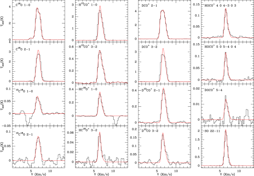
Figure 14: Spectra as observed with the IRAM 30-m telescope. The scale is in main beam brightness temperature. Negative features are artefacts of the frequency switching observing procedure. In red, the fits shown in Table B.1.

Figures 14 to  22 show the spectra of the neutral and protonated species considered in this work. In all cases, the protonated and neutral species present similar line profiles suggesting that both come from the same region. All the lines show two narrow velocity components, at $\sim$6.5 km s^-1 and $\sim$7.0 km s^-1, respectively. We use the 30 m maps to explore the origin of the different species and the two velocity components. The integrated intensity maps of the SO 2₂$\rightarrow$1₁, C³⁴S 3$\rightarrow$2, HCS⁺ 2$\rightarrow$1, HC¹⁸O⁺ 1$\rightarrow$0, HOCO⁺ 4₀₄$\rightarrow$3₀₃, DCO⁺ 2$\rightarrow$1, D¹³CO⁺ 2$\rightarrow$1, p-H₂CO 2₀₂$\rightarrow$2₀₁, and p-H₂¹³CO 2₀₂$\rightarrow$2₀₁ lines are shown in Fig. 2. The emission of the HC¹⁸O⁺, HOCO⁺, C³⁴S, DCO⁺, D¹³CO⁺, and SO lines is concentrated in the elongated filament that contains B1b-N and B1b-S (see Fig. 2). The emission of the N₂H⁺ 1$\rightarrow$0 line, as reported by Daniel et al. (2013), is also concentrated in this dense filament. In the case of HOCO⁺, the elongated emission seems to be slightly shifted to the west although the map is too noisy to conclude. In all these cases, the line intensities are similar toward the N and S protostars. On the contrary, the emission of the o-NH₂D 1${}_{11}s$$\rightarrow$0${}_{01}a$ line peaks toward B1b-N (Daniel et al., 2013). Another exception is H₂CO whose emission presents an intense peak toward B1b-S. The emission of the HCS⁺ 2$\rightarrow$1 line presents a flat spatial distribution suggesting that this emission is coming from the cloud envelope.

Linewidths can also provide information about the origin of the molecular emission. On basis of low angular resolution observations, Bachiller et al. (1990) proposed a correlation between the linewidths and the depth into the B1 cloud with the narrowest lines ($\sim$1 km s^-1) coming from the highest extinction regions. Similar results were obtained by Daniel et al. (2013) on basis of the observation of HCN, HNC, N₂H⁺, NH₃, and their isotopologues. The line profiles were well reproduced by a collapsing dense core (infall velocity = 0.1 km s^-1) with a turbulent velocity of 0.4 km s^-1 surrounded by a static lower density envelope with a turbulent velocity of 1.5 km s^-1. In Fig. 3, we show the spatial distribution of the linewidths for the set of maps shown in Fig. 2. In agreement with previous works, we find a clear decrease of the linewidth with the distance from the core center in the SO 2₂$\rightarrow$1₁ line. Linewidths are $\sim$2 km s^-1 in the most external layer and decrease to $\sim$0.7 km s^-1 toward the core center. However, the linewidths of the HCS⁺ 2$\rightarrow$1 lines are $\sim$2 km s^-1 all over the region without a clear pattern. This supports the interpretation of the HCS⁺ emission coming from an external layer of the cloud. The only position where the linewidths of the HCS⁺ line becomes $<$1 km s^-1 is toward the IR star B1b-W. For HC¹⁸O⁺, DCO⁺, and D¹³CO⁺, we do see a trend, with the linewidths decreasing with the decreasing radius from the core center. However, their linewidths are always $>$1 km s^-1 suggesting that the emission is not dominated by the innermost layers of the envelope. The linewidth of the p-H₂CO line is very constant over the whole core. This line is more likely to be optically thick and its emission is only tracing the outer layers of the core.

Figures 4 and 5 show the spectral maps of the DCO⁺ 2$\rightarrow$1 and SO 2₂$\rightarrow$1₁ lines, respectively. The emission of DCO⁺ extends from $\sim$5.5 km s^-1 to $\sim$8.0 km s^-1, while the SO emission is detected in a narrower velocity range between $\sim$5.9 km s^-1 to $\sim$7.5 km s^-1, i.e., SO is mainly coming from the 6.5 km s^-1 component. The intensity peak at 6.5 km s^-1 is shifted $\sim$5^′′ west from the peak at 7.0 km s^-1. It is interesting to note that DCO⁺ presents an emission peak toward B1b-N at a velocity of $\sim$7.5 km s^-1 in agreement with the N₂H⁺ and NH₂D observations by Daniel et al. (2013). Recent interferometric observations revealed the kinematical structure of this region at scales of $\sim$500-1000 AU (Huang & Hirano, 2013; Gerin et al., 2015). Huang & Hirano (2013) detected intense emission of the N₂D⁺ 3$\rightarrow$2 lines toward the two protostellar cores B1b-N and B1b-S using the SMA. The N₂D⁺ emission is centered at $\sim$7.0$\pm$0.2 km s^-1 toward B1b-N and at $\sim$6.5$\pm$0.2 km s^-1 toward B1b-S, confirming the existence of the two velocity components.

In the cases of H₂¹³CO, H₂S, HOCO⁺, and in one transition of CCS, OCS, and SO₂ (see Table B.1), we detect wings at redshifted velocities. Compact outflows are detected toward each protostellar core with wings in the 0 to 15 km s^-1 velocity range (Gerin et al., 2015). In Fig. 6 we overlay the 30 m beam at 3 mm and 1 mm on the interferometric H₂CO map. The B1b-N outflow and the red wing of the B1b-S outflow lie within our beam at 3 mm, but the whole B1b-N outflow and a fraction of the red lobe of the B1b-S outflow are missed in the 2 mm and 1 mm observations. The emission at the outflow velocities is not taken into account in our calculations because we are only interested in the two velocity components associated with the core emission (see Sect. 5 for details).

Table 2: Column density calculations

Molecule	LTE					LVG1
	6.5 km s-1		7.0 km s-1		Total	6.5 km s-1	7.0 km s-1	Total
	Trot(K)	NX(cm-2)	Trot(K)	NX(cm-2)	NX(cm-2)	NX(cm-2)	NX(cm-2)	NX(cm-2)
Ions						Ions
HC18O+	4.4${}_{-0.2}^{+0.2}$	1.7${}_{-0.1}^{+0.1}$$\times$1011	4.2${}_{-0.7}^{+0.4}$	1.5${}_{-0.3}^{+0.2}$$\times$1011	3.2$\times$1011	2.0${}_{-0.1}^{+0.1}$$\times$1011	1.4${}_{-0.3}^{+0.2}$$\times$1011	3.4$\times$1011
D13CO+	7.8${}_{-0.5}^{+0.5}$	1.2${}_{-0.2}^{+0.2}$$\times$1011	4.5${}_{-0.2}^{+0.2}$	3.9${}_{-0.5}^{+0.5}$$\times$1011	5.1$\times$1011	2.0${}_{-0.1}^{+0.1}$$\times$1011	4.5${}_{-0.1}^{+0.1}$$\times$1011	6.5$\times$1011
HOCO+	11.9${}_{-0.3}^{+0.3}$	5.2${}_{-0.3}^{+0.3}$$\times$1011	10.7${}_{-1.0}^{+1.3}$	2.4${}_{-0.7}^{+1.0}$$\times$1011	7.6$\times$1011	5.2${}_{-0.2}^{+0.2}$$\times$1011	3.0${}_{-0.2}^{+0.2}$$\times$1011	8.2$\times$1011
DOCO+	11a	7.0${}_{-0.9}^{+0.9}$$\times$1010	11a	4.0${}_{-2.0}^{+2.0}$$\times$1010	1.1$\times$1011	9.0${}_{-1.1}^{+1.1}$$\times$1010	5.0${}_{-2.0}^{+2.0}$$\times$1010	1.1$\times$1011
SO+	9.0${}_{-0.7}^{+0.8}$	7.6${}_{-1.6}^{+2.0}$$\times$1011	8.3${}_{-1.4}^{+2.2}$	4.8${}_{-2.2}^{+4.1}$$\times$1011	1.2$\times$1012
HCS+	10.6${}_{-3.0}^{+6.5}$	2.1${}_{-1.3}^{+3.6}$$\times$1011	7.5${}_{-0.6}^{+0.5}$	6.2${}_{-0.2}^{+0.2}$$\times$1011	8.3$\times$1011	5.5${}_{-0.1}^{+0.1}$$\times$1011	5.5${}_{-0.1}^{+0.1}$$\times$1011	1.1$\times$1012
DCS+	10b	5.0${}_{-1.0}^{+1.0}$$\times$1010			5.0$\times$1010	4.5${}_{-1.1}^{+1.1}$$\times$1010		4.5$\times$1010
HCNH+	29.0${}_{-12}^{+50}$	5.1${}_{-0.7}^{+4.1}$$\times$1012	8.9${}_{-2.9}^{+5.3}$	3.8${}_{-0.5}^{+1.5}$$\times$1012	8.9$\times$1012	3.7${}_{-0.4}^{+0.4}$$\times$1012	4.0${}_{-0.4}^{+0.4}$$\times$1012	7.7$\times$1012
H2COH+			10a	2.0${}_{-1.0}^{+1.0}$$\times$1011	2.0${}_{-1.0}^{+1.0}$$\times$1011
CO+			10a	$<$6.0$\times$1010	$<$6.0$\times$1010
HOC+			10a	$<$2.0$\times$1010	$<$2.0$\times$1010
Neutrals						Neutrals
13C18O	5.5${}_{-0.9}^{+1.3}$	2.4${}_{-0.2}^{+0.2}$$\times$1013	10.9${}_{-1.4}^{+0.9}$	5.2${}_{-0.1}^{+0.1}$$\times$1013	7.6$\times$1013	3.0${}_{-0.2}^{+0.2}$$\times$1013	6.0${}_{-0.3}^{+0.3}$$\times$1013	9.0$\times$1013
o-H213CO	5.5${}_{-0.6}^{+0.8}$	6.1${}_{-1.5}^{+2.1}$$\times$1011	5.2${}_{-0.3}^{+0.9}$	4.9${}_{-1.9}^{+3.2}$$\times$1011	1.1$\times$1012	1.1${}_{-0.6}^{+0.6}$$\times$1012	1.3${}_{-0.7}^{+0.7}$$\times$1012	2.4$\times$1012
13CS	7.1${}_{-1.1}^{+1.6}$	7.8${}_{-5.7}^{+2.0}$$\times$1011	3.2${}_{-0.7}^{+0.4}$	3.1${}_{-1.6}^{+3.2}$$\times$1012	3.9$\times$1012	1.3${}_{-0.1}^{+0.1}$$\times$1012	9.0${}_{-0.3}^{+0.3}$$\times$1011	2.2${}_{-0.1}^{+0.1}$$\times$1012
S18O	6.8${}_{-0.6}^{+0.6}$	1.6${}_{-0.5}^{+0.6}$$\times$1012	8.2${}_{-1.4}^{+2.0}$	0.6${}_{-0.3}^{+0.4}$$\times$1012	2.3$\times$1012	2.2${}_{-0.1}^{+0.1}$$\times$1012	8.0${}_{-0.3}^{+0.3}$$\times$1011	3.0$\times$1012
33SO	12.3${}_{-4.0}^{+7.3}$	1.6${}_{-0.6}^{+1.0}$$\times$1012	18.9${}_{-8.3}^{+71}$	0.7${}_{-0.4}^{+0.7}$$\times$1012	2.3$\times$1012	3.8${}_{-0.1}^{+0.1}$$\times$1012	6.0${}_{-2.0}^{+2.0}$$\times$1011	4.4$\times$1012
34SO2	5.8${}_{-1.2}^{+2.0}$	1.1${}_{-0.5}^{+1.0}$$\times$1012				1.1${}_{-0.1}^{+0.1}$$\times$1012
SO2	10.1${}_{-1.0}^{+1.0}$	7.9${}_{-2.0}^{+3.0}$$\times$1012	10.2${}_{-1.2}^{+2.0}$	2.9${}_{-0.9}^{+1.3}$$\times$1012	1.1$\times$1013	1.6${}_{-0.1}^{+0.1}$$\times$1013	4.5${}_{-0.1}^{+0.1}$$\times$1012	2.0$\times$1013
OC34S	8.7${}_{-0.5}^{+0.6}$	1.2${}_{-0.2}^{+0.2}$$\times$1012				1.0${}_{-0.3}^{+0.3}$$\times$1012
OCS	11.7${}_{-4.0}^{+13.0}$	1.5${}_{-0.6}^{+0.9}$$\times$1013	20.4${}_{-1.3}^{+1.4}$	4.9${}_{-0.6}^{+0.6}$$\times$1012	1.9$\times$1013	1.7${}_{-0.1}^{+0.1}$$\times$1013	8.0${}_{-4.0}^{+4.0}$$\times$1011	1.7$\times$1013
H213CSc	7.4	1.6${}_{-0.3}^{+0.3}$$\times$1011
CCS	8.3${}_{-0.6}^{+0.7}$	5.9${}_{-1.7}^{+2.4}$$\times$1012	8.2${}_{-0.6}^{+0.7}$	3.6${}_{-1.0}^{+1.3}$$\times$1012	9.5$\times$1012	9.3${}_{-0.1}^{+0.1}$$\times$1012	5.2${}_{-0.1}^{+0.1}$$\times$1012	1.4$\times$1013
CC34S						3.5${}_{-0.7}^{+0.7}$$\times$1011	2.5${}_{-0.7}^{+0.7}$$\times$1011	6.0$\times$1011
CCCS
C13CCS
o-H2S	10d	7.0${}_{-0.2}^{+0.2}$$\times$1012	10	3.0${}_{-0.2}^{+0.2}$$\times$1012	1.0$\times$1013
NS	10d	5.4${}_{-0.2}^{+0.2}$$\times$1012	10	9.0${}_{-0.2}^{+0.2}$$\times$1012	1.4$\times$1013

¹ LVG calculations assuming T_k=12 K and n(H₂)=10⁵ cm^-3; ^a Assuming the rotation temperature of HOCO⁺; ^b Assuming the rotation temperature of HCS⁺; ^c In this case the ortho and para species are treated together (ortho-to-para(OTP)=3) and we assumed the rotation temperature calculated for H₂CS by Marcelino et al. (2005); ^d Reasonable guess for the rotation temperature.

Table 3: Fractional abundances and abundance ratios

Molecule	LTE			LVG1
	6.5 km s-1	7.0 km s-1	Total	6.5 km s-1	7.0 km s-1	Total
Ions				Ions
X(HC18O+)$\times$550	3.9$\times$10-9	1.8$\times$10-9	2.5$\times$10-9	4.6$\times$10-9	1.7$\times$10-9	2.7$\times$10-9
X(D13CO+)$\times$60	2.7$\times$10-10	4.7$\times$10-10	4.0$\times$10-10	4.6$\times$10-10	5.4$\times$10-10	5.1$\times$10-10
X(HOCO+)	2.0$\times$10-11	4.8$\times$10-12	1.0$\times$10-11	2.0$\times$10-11	6.0$\times$10-12	1.1$\times$10-11
X(DOCO+)	2.9$\times$10-12	8.0$\times$10-13	1.4$\times$10-12	3.6$\times$10-12	1.0$\times$10-12	1.4$\times$10-12
X(SO+)	3.1$\times$10-11	9.6$\times$10-12	1.6$\times$10-11
X(HCS+)	8.1$\times$10-12	1.2$\times$10-11	1.1$\times$10-11	2.1$\times$10-11	1.1$\times$10-11	1.4$\times$10-11
X(DCS+)	1.9$\times$10-12		6.6$\times$10-13	1.7$\times$10-12		5.9$\times$10-13
X(HCNH+)	2.0$\times$10-10	7.6$\times$10-11	1.2$\times$10-10	1.4$\times$10-10	8.0$\times$10-11	1.0$\times$10-10
X(H2COH+)		4.0$\times$10-12	2.6$\times$10-12
X(CO+)			$<$7.9$\times$10-13
X(HOC+)			$<$2.6$\times$10-13
X(NNH+)			1.4$\times$10-9∗
X(NND+)			5.0$\times$10-10∗
Neutrals				Neutrals
X(13C18O)	1.0$\times$10-9	1.0$\times$10-9	1.0$\times$10-9	1.2$\times$10-9	1.2$\times$10-9	1.2$\times$10-9
X(H213CO)$\times$60a	1.9$\times$10-9	7.8$\times$10-10	1.1$\times$10-9	3.4$\times$10-9	2.1$\times$10-9	2.5$\times$10-9
X(13CS)$\times$60	1.8$\times$10-9	3.7$\times$10-9	3.1$\times$10-9	3.0$\times$10-9	1.1$\times$10-9	1.7$\times$10-9
X(S18O)$\times$550	3.7$\times$10-8	6.3$\times$10-9	1.8$\times$10-8	5.0$\times$10-8	9.0$\times$10-9	2.2$\times$10-8
X(33SO)$\times$135	9.0$\times$10-9	1.8$\times$10-9	4.0$\times$10-9	1.9$\times$10-8	1.6$\times$10-9	7.9$\times$10-9
X(34SO2)$\times$22.5	1.0$\times$10-9			1.0$\times$10-9
X(SO2)	3.3$\times$10-10	5.6$\times$10-11	1.4$\times$10-10	6.7$\times$10-10	9.0$\times$10-11	2.6$\times$10-10
X(OC34S)$\times$22.5	1.1$\times$10-9			9.4$\times$10-10
X(OCS)	6.2$\times$10-10	9.4$\times$10-11	2.4$\times$10-10	7.0$\times$10-10	1.5$\times$10-11	2.2$\times$10-10
X(H213CS)$\times$60	4.0$\times$10-10
X(CCS)	2.4$\times$10-10	6.9$\times$10-11	1.2$\times$10-10	3.9$\times$10-10	1.0$\times$10-10	1.8$\times$10-10
X(H2S)a	3.9$\times$10-10	7.7$\times$10-11	1.7$\times$10-10
X(NS)	2.2$\times$10-10	1.7$\times$10-10	1.8$\times$10-10
X(HCN)			1.2$\times$10-8∗
Ion/Neutral and Ion/Ion				Ion/Neutral and Ion/Ion
$\frac{N(HCO^{+})}{N(CO)}$	1.1$\times$10-4	4.8$\times$10-5	6.9$\times$10-5	1.1$\times$10-4	4.3$\times$10-5	6.8$\times$10-5
$\frac{N(DCO^{+})}{N(HCO^{+})}$	0.07	0.26	0.15	0.1	0.32	0.19
$\frac{N(DCO^{+})}{N(CO)}$	9.0$\times$10-6	1.2$\times$10-5	1.1$\times$10-5	1.1$\times$10-5	1.4$\times$10-5	1.2$\times$10-5
$\frac{N(HOCO^{+})}{N(HCO^{+})}$	0.005	0.003	0.004	0.004	0.003	0.004
$\frac{N(SO^{+})}{N(SO)}$	8.0$\times$10-4	0.0014	9.5$\times$10-4
$\frac{N(HCS^{+})}{N(CS)}$	0.004	0.003	0.0035	0.007	0.01	0.008
$\frac{N(DCS^{+})}{N(HCS^{+})}$	0.24		0.06	0.08		0.04
$\frac{N(HCS^{+})}{N(HCO^{+})}$	0.003	0.007	0.004	0.004	0.006	0.005
$\frac{N(HCNH^{+})}{N(HCN)}$			0.01			0.008
$\frac{N(H_{2}COH^{+})}{N(H_{2}CO)}$		0.005	0.002
$\frac{N(CO^{+})}{N(HCO^{+})}$			$<$3$\times$10-4
$\frac{N(HOC^{+})}{N(HCO^{+})}$			$<$1$\times$10-4
Neutral/Neutral				Neutral/Neutral
$\frac{N(SO)}{N(CS)}$	19	1.8	5	17	8	13
$\frac{N(SO_{2})}{N(SO)}$	0.03	0.008	0.008	0.01	0.009	0.01
$\frac{N(CCS)}{N(CS)}$	0.13	0.02	0.04	0.12	0.09	0.11
$\frac{N(H_{2}CS)}{N(CS)}$	0.20
$\frac{N(OCS)}{N(CS)}$	0.57	0.03	0.08	0.22	0.01	0.13

¹ LVG calculations assuming T_k=12 K and n(H₂)=10⁵ cm^-3; numbers in boldface are used in Fig. 7 to Fig. 11 to compare with observations. ^∗ From Daniel et al. (2013); ^a From Table 2 assuming OTP=3.

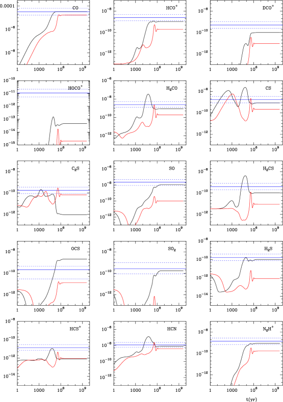
Figure 7: Results of our best-fit model ($\zeta_{H_{2}}$=4.0$\times$10^-17 s^-1, O/H=3.0 10^-5, N/H=6.4 10^-5, C/H=1.7 10^-5, and S/H=6.0 10^-7). We assume a density of n(H₂)=10⁵ cm^-3 and T_k=12 K. The thick and dashed blue lines indicate the observed values and their uncertainty, which are considered to be a factor of 2 for most molecules (see text), respectively. In the case of SO, SO₂, and OCS, their abundances change by more than a factor of 2 between the 6.5 km s^-1 and 7.0 km s^-1 velocity components. In the panels corresponding to these species, the dashed lines indicate the abundance for each component separately. In red we show model calculations for the same conditions and n(H₂)=10⁴ cm^-3.

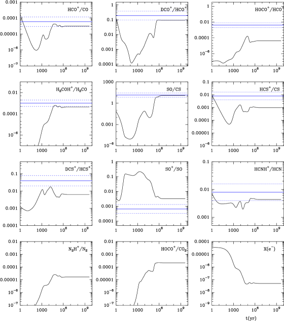
Figure 8: Results of our best-fit model ($\zeta_{H_{2}}$=4.0$\times$10^-17 s^-1, O/H=3.0 10^-5, N/H=6.4 10^-5, C/H=1.7 10^-5, and S/H=6.0 10^-7). We assume a density of n(H₂)=10⁵ cm^-3 and T_k=12 K. The thick and dashed blue lines indicate the observed values and their uncertainties.

5 Column density calculations

In order to investigate abundance variations between the two velocity components, we carried out a separate analysis for each. The spectral resolution of our observations is different for the 3 mm, 2 mm and 1 mm bands. To carry out a uniform analysis, we degraded the velocity resolution to a common value of 0.25 km s^-1 and then fitted Gaussians to each one. In the fitting, we fixed the central velocities to 6.5 km s^-1 and $\sim$7.0 km s^-1, and the linewidths to $\Delta$v=0.7 km s^-1 and 1.0 km s^-1, respectively. The fitting returns the integrated intensity for each component. This procedure gives an excellent fit for most lines and neglects possible line wings with velocities $>$7.5 km s^-1. The final integrated intensities are shown in Table B.1. We are aware that this simple method is not able to cleanly separate the contribution from each component. There is some unavoidable velocity overlap between the two components along the line of sight and our spatial resolution is limited (see Fig 4 and Fig 5). In spite of that, our simple method help to detect possible chemical gradients.

Several isotopologues of each molecule were detected as expected taking the large extinction in this core into account (A_v$\sim$76 mag). As zero-order approximation, we derived the column densities and fractional abundances of the different species using the rotation diagram technique. This technique gives a good estimate of the total number of molecules within our beam as far as the observed lines are optically thin. To be sure of this requirement, we selected the rarest isotopologue of each species. Furthermore, we assumed that the emission is filling the beam. To calculate the column densities and abundances of the main isotopologues, we adopted ¹²C/¹³C=60, ¹⁶O/¹⁸O=550, ³²S/³⁴S=22.5, and ³⁴S/³³S=6 (Chin et al., 1996; Wilson et al., 1999).

In Table 2 we show the results of our rotational diagram calculations. The errors in the rotation temperatures and column densities are those derived from the least squares fitting. There are, however, other kind of uncertainties that are not considered in these numbers. One source of uncertainty is the unknown beam filling factor. Since the beam is dependent on the frequency, this could bias the derived rotation temperature. To estimate the error from this uncertainty, we calculated the column densities with an alternative method. Daniel et al. (2013) modeled the density structure of the Barbard 1b core on the basis of dust continuum at 350 $\mu$m and 1.2 mm. These authors obtained that the mean density in the $\sim$29$\arcsec$ beam is n(H₂)$\approx$10⁵ cm^-3. Lis et al. (2010) derived a gas kinetic temperature of T_K = 12 K from NH₃ observations. We adopted these physical conditions to derive the molecular column densities by fitting the integrated intensity of the lowest energy transition using the LVG code MADEX (Cernicharo, 2012). The results are shown in Table 2. Column densities derived using the rotation diagram technique and LVG calculations agree within a factor of 2 for all the compounds. We consider that our estimates are accurate within this factor.

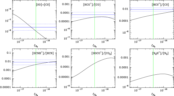
Figure 9: Steady-state calculations of fractional abundances and abundance ratios. All the input parameters except $\zeta_{H_{2}}$ are the same as in Fig. 7. Horizontal blue lines correspond to the observed values and their uncertainty that is considered a factor of 2. Vertical green lines indicate the estimated value of the cosmic ray ionization rate, $\zeta_{H_{2}}$=4$\times$10^-17 s^-1.

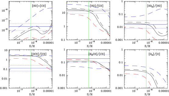
Figure 10: Steady-state calculations of fractional abundances and abundance ratios. All the input parameters except S/H are the same as in Fig. 7. Horizontal blue lines correspond to the observed values and their uncertainty. Vertical green lines indicate the estimated value of the sulfur elemental abundance, S/H=6$\times$10^-7. The solid black line represents our best model fit, $\zeta_{H_{2}}$=4$\times$10^-17 s^-1. The dashed blue, black, and red lines correspond to $\zeta_{H_{2}}$=1, 4 and 10$\times$10^-17 s^-1, respectively.

Figure 11: Predicted fractional abundances using the same parameters as in Fig 7. The abundances of SO, SO₂ and SO⁺, and O₂ dramatically increase after 1 Myr.

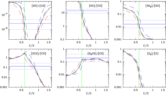
Figure 12: Steady-state calculations of fractional abundances and abundance ratios. All the input parameters except O/H are the same as in Fig. 7. Horizontal blue lines correspond to the observed values and their uncertainty. Vertical green lines indicate the estimated value of C/O elemental ratio, C/O=0.6. The dashed blue, black, and red lines correspond to $\zeta_{H_{2}}$=1, 4 and 10$\times$10^-17 s^-1, respectively.

In Table 3 we show the fractional abundances of the studied species and some interesting molecular abundance ratios. To estimate the fractional abundances for each velocity component, we assumed that the abundance of ¹³C¹⁸O is the same for the two components and adopted a total molecular hydrogen column density of N(H₂)=7.6 10²² cm^-2 (Daniel et al., 2013). Most of the fractional abundances and abundance ratios agree within the uncertainties for the two velocity components. There are, however, significant chemical differences for some species. One difference is that the HCO⁺ deuterium fraction is a factor $\sim$3 higher in the 7 km s^-1 component than in the 6.5 km s^-1 one. The spectral velocity maps of the DCO⁺ 2$\rightarrow$1 and D¹³CO⁺ 2$\rightarrow$1 lines show that the 7 km s^-1 component is associated with the cold protostar B1b-N. The second difference is that the SO/CS abundance ratio is 2$-$10 times larger in the $\sim$6.5 km s^-1 component than in the $\sim$7.0 km s^-1 component. High SO abundances, up to $\sim$10^-7, are found in bipolar outflows because of the release of sulfuretted compounds into the gas phase (Bachiller & Pérez Gutiérrez, 1997). One could think that the high SO abundances could then result from the interaction of the cold core with the B1b-S outflow, or, more likely, of the interaction of the dense core with the B1a and/or B1d outflows. However, the profiles of the SO lines are very narrow, which is contrary to one would expect if the emission were coming from a shock or a turbulent medium. In Sect. 6, we discuss in detail the sulfur chemistry and possible explanations for the high SO abundance in Barnard 1.

One important result is that the [XH⁺]/[X] ratios do not present variations between the two velocity components. This supports our interpretation that the ionization fraction is mainly driven by CR and is consistent with the measured H₂ column density (7.6$\times$10²² cm^-2). The core is expected to be thoroughly permeable to CR and the ionization does not present significant fluctuations across the envelope.

6 Chemical modeling

We perform chemical modeling to constrain the physical and chemical properties in Barnard B1b. We do not include here the accretion/desorption mechanisms of gas-phase molecules on the grains and instead vary the amount of elemental abundances of heavy atoms available in the gas phase to mimic these effects. We explicitly consider, however, the formation on grains of the molecular hydrogen, H₂, and the isotopic substituted forms HD and D₂. Such an approach, although primitive, allows us to disentangle the main gas-phase processes at work. We use both a steady-state and time-dependent model to explore the chemistry and verified that the steady-state results are recovered by the time-dependent code for sufficiently large evolution time (typically 10 Myr).

Our chemical network contains 261 species linked through more than 5636 chemical reactions. Ortho and para forms of H₂, H${}_{2}^{+}$, H${}_{3}^{+}$, D₂, H₂D⁺, D₂H⁺, and D${}_{3}^{+}$ are explicitly introduced, following the pioneering papers of Flower et al. (2004, 2006) for heavily depleted regions, and including the chemistry of carbon, oxygen, nitrogen, and sulfur. Discriminating between para and ortho forms of H₂ is particularly critical for deuteration in cold regions via the H${}_{3}^{+}$ + HD $\leftrightarrow$ H₂D⁺ + H₂ reaction as the endothermicity of the reverse reaction is of the same order of magnitude as the rotational energy of H₂, as first emphasized by Pagani et al. (1992). Nitrogen chemistry is also very sensitive to the ortho and para forms of H₂, as pointed out by Le Bourlot (1991), because of the small endoergicity of the N⁺ + H₂ $\rightarrow$ NH⁺ + H reaction. Whereas a definitive understanding of this reaction is still pending (Zymak et al., 2013), we follow the prescription of Dislaire et al. (2012) for the reaction rate coefficients of N⁺ + H₂(p/o) reaction. Our chemical network also contains the recent updates coming from experimental studies of reactions involving neutral nitrogen atoms as reviewed in Wakelam et al. (2013). We also introduced species containing two nitrogen atoms, such as C₂N₂ and C₂N₂H⁺, following the recent detection of C₂N₂H⁺ by Agúndez et al. (2015) for which the reaction rate coefficients have essentially been taken from the UMIST astrochemical database (McElroy et al., 2013). An important feature that is not fully recognized is the link between sulfur and nitrogen chemistry as shown by the detection of NS, which is found both in regions of massive star formation and in cold dark clouds (McGonagle et al., 1994; McGonagle & Irvine, 1997). The main formation reaction is through S + NH whose rate is given as 10^-10 cm³ s^-1 in astrochemical databases, which then also induces that sulfur chemistry may depend on o/p ratio of H₂.

Our methodology is the following: We run the time-dependent model for a set of standard elemental abundances and cosmic ray ionization rates to determine which molecular abundances and molecular abundance ratios reach the steady state in a few 0.1$-$1 Myr, which is the estimated age for Barnard B1b. These molecular abundances and abundance ratios are expected to be in equilibrium and are used to explore the parameter space using steady-state calculations. On basis of the steady-state calculations, we select the most plausible values and run the time-dependent model to confirm that our fit is correct. In all our calculations, we assume uniform physical conditions and fix n(H₂)=10⁵ cm^-3 and T_k=12 K, according with previous works (Lis et al., 2010; Daniel et al., 2013). We iterate several times to get the best match with the observations. The predictions of our best-fit model are compared with observations in Figs. 7 and  8.

6.1 Cosmic ray ionization rate

The [HCO⁺]/[CO] ratio has been extensively used to estimate the cosmic ray ionization rate. The results of our time dependent model confirms that it is, very likely, the most reliable diagnostic since it reaches the equilibrium in 0.1 Myr and its chemistry is well known. Other [XH⁺]/[X] ratios, such as [HCS⁺]/[CS] and [HCNH⁺]/[HCN], are also expected to be in equilibrium at the typical ages of a molecular cloud. Figure 9 shows the variation of the [HCO⁺]/[CO], [HCNH⁺]/[HCN], and [HCS⁺]/[CS] as a function of the cosmic ray ionization rate in steady-state calculations. Assuming an uncertainty of a factor of 2 in the derived abundance ratios, values of $\zeta_{H_{2}}$ in the interval between 3$\times$10^-17 s^-1 to 1$\times$10^-16 s^-1 are consistent with the observed [HCO⁺]/[CO] and [HCNH⁺]/[HCN] ratios. These values are at the upper end of the values inferred for cloud cores (Caselli et al., 1998) and are higher than those of the typical dark cloud L1544, $\zeta_{H_{2}}$ $\sim$1$\times$10^-18 (Galli & Padovani, 2015). This could explain the higher gas and dust temperature in this dense core of T_d$\sim$12 K, compared with dust temperature in L1544 of T_d$<$6$-8$ K (Crapsi et al., 2007).

The [HCS⁺]/[CS] ratio is not fitted by any reasonable value of $\zeta_{H_{2}}$. This is not surprising since the HCS⁺ emission is mainly coming from the low density envelope. In Fig. 7 we show model predictions for a density of n(H₂)=10⁴ cm^-3. The abundances of most molecules decrease while the HCS⁺ abundance remains constant and that of CCS increases. These calculations were carried out assuming the same elemental abundances as in the high density case. This is not realistic since lower depletions are expected in the envelope and, therefore, the HCS⁺ abundance would be higher. Moreover, this core is illuminated on its eastern side by the nearby Herbig Ae stars LkH$\alpha$ 327 and LkH$\alpha$ 328 (Walawender et al., 2009; Young et al., 2015). The UV photons are expected to increase the HCS⁺ abundance. In fact, the HCS⁺ 2$\rightarrow$1 emission is maximum toward the illuminated side (see Fig. 2).

Our estimate of the cosmic ray ionization rate permits us to obtain an estimate of the N₂ abundance in this core. Since it is one of the main nitrogen reservoirs, N₂ cannot be observed at (sub)millimeter wavelengths because of its lack of dipole moment. We can only estimate its abundance indirectly through the protonated compound, N₂H⁺. The N₂H⁺ abundance is very sensitive to the cosmic ray ionization rate. In Fig. 9, we present the [N₂H⁺]/[N₂] ratio as a function of the cosmic ray ionization rate. Assuming $\zeta_{H_{2}}$=4$\times$10^-17 s^-1 and on the basis of our observational data, we derive [N₂]$\sim$8$\times$10^-5, which is consistent with the typical value of the N elemental abundance in a dark cloud, N/H=6.4$\times$10^-5.

The HOCO⁺ molecule (protonated carbon dioxide) is thought to form via a standard ion-molecule reaction, the transfer of a proton from H${}_{3}^{+}$ to CO₂ (see, e.g., Turner et al., 1999). To date HOCO⁺ has been detected toward the Galactic center, a few starless translucent clouds (Turner et al., 1999), a single low-mass Class 0 protostar (Sakai et al., 2008), and the protostellar shock L1157-B1 (Podio et al., 2014). Interestingly, this molecule is particularly abundant, $\sim$10^-9, in the Galactic center region (Minh et al., 1988, 1991; Deguchi et al., 2006; Neill et al., 2014). We derive an HOCO⁺ abundance of $\sim$10^-11, i.e, two orders of magnitude lower than that derived in the Galactic center clouds (Deguchi et al., 2006; Neill et al., 2014) and L1157-B1 (Podio et al., 2014), and a factor of $\sim$10 lower than that in translucent clouds (Turner et al., 1999). This is not unexpected sine the HOCO⁺ abundance is inversely proportional to the gas density (Sakai et al., 2008) and B1b is a dense core. Our model underpredicts the HOCO⁺ abundance by a factor 200 (see Fig. 7). As commented below, HOCO⁺ is proxy of CO₂, which is not efficiently formed in the gas phase (Turner et al., 1999).

The lack of an electric dipole moment of CO₂ makes gas-phase detections difficult. The abundance of CO₂ in the solid phase has been investigated through its two vibrational modes at 4.3 and 15.0 $\mu$m. In the solid phase, the typical abundance is $\sim$10^-6 relative to total H₂ (Gerakines et al., 1999; Gibb et al., 2004). In the gas phase, the typical detected abundance is 1$-$3$\times$10^-7 (van Dishoeck et al., 1996; Boonman et al., 2003; Sonnentrucker et al., 2006). Assuming the [HOCO⁺]/[CO₂] ratio predicted by our model, 2.2$\times$10^-4, we estimate a CO₂ abundance of $\sim$5$\times$10^-8. This value is at the lower end of those measured in star-forming regions but 200 times larger than that predicted by our gas-phase model. Photodesorption and sputtering of the icy mantles are more likely to be the main CO₂ production mechanisms.

6.2 Sulfur chemistry: C, O, and S elemental abundances

The initial elemental abundances in the gas phase are an essential parameter in the chemical modeling. In cloud cores (A_v$>$10 mag), as long as the C elemental abundance is lower than O, we can assume that the abundance of C is equal to that of CO and conclude that C/H=1.7$\times$10^-5; we note that fractional abundances are given with respect to H₂. The main source of uncertainty in this value comes from the uncertainty in the CO abundance, which is estimated to be a factor of 2.

To estimate the amount of S in the gas phase requires a detailed modeling of its chemistry. As shown in Fig. 10, the cosmic ray ionization rate is a critical paramenter to estimate the S/H. The main sulfur reservoirs in a dense core are atomic sulfur (S) and SO (see Fig. 11). Unfortunately, chemical models make a poor work in predicting the fractional abundance of SO, because the predicted SO abunance depends on two uncertain factors: i) the S + O₂ $\rightarrow$ SO + O and S + OH $\rightarrow$ SO + H reaction rates and ii) the O₂ and OH abundances.

Table 4: Elemental abundances relative to H

Solar			Dark cloud: TMC11		Barnard 1b2
	X/H3	fD4	X/H	fD	X/H	fD
C	1.4 10-4	$\sim$1	1.4 10-4	$\sim$1	1.7 10-5	$\sim$8
O	3.1 10-4	$\sim$1	1.3 10-4	$\sim$2	3.0 10-5	$\sim$10
N	7.7 10-5	$\sim$1	6.2 10-5	$\sim$1	6.4 10-5	$\sim$1
S	1.5 10-5	$\sim$1	8.0 10-8	$\sim$200	6.0 10-7	$\sim$25

¹ From the compilation by Agúndez & Wakelam (2013); ² This work;
³ Elemental abundance in the gas phase; ⁴ Depletion factor = (X/H)_⊙/(X/H).

The S + O₂ reaction rate coefficient at low temperatures is not known. Experimental measurements have only been performed above 200 K. Lu et al. (2004) reviewed the various theoretical and experimental results and adopted a value of 2 $\times$ 10^-12 cm³ s^-1 at 298 K. The UMIST and KIDA databases suggest different values. In KIDA, a constant value of 2.1 $\times$ 10^-12 cm³ s^-1 is suggested in the 250$-$430 K temperature range whereas the latest version of the UMIST database gives 1.76 $\times$ 10^-12 (T/300)^0.81 exp(30.8/T) cm³ s^-1 in the 200$-$3460 K temperature interval. This small activation barrier would imply rates as low as 10^-23 cm³ s^-1 at the temperature of 12 K and a decrease in the SO, SO₂, and SO⁺ abundances. Quasiclassical trajectory calculations were carried out for the reaction S + O₂ and its reverse by Rodrigues & Varandas (2003). With 6000 trajectories they obtain that the reaction rate remains constant or decreases very slowly for temperatures between 50 K and 1000 K. Using the same potential, we performed new quasiclassical trajectory calculations with 100 000 trajectories for temperatures between 10 K and 50 K (see Appendix A). Our results confirm that the reaction rate remains very constant (within 30%) in the 10 K to 50 K range. Therefore, we adopted the KIDA value, 2.1 $\times$ 10^-12 cm³ s^-1, in our calculations.

The second more important reaction for the formation of SO is S + OH. DeMore et al. (1997) measured a value of 6.6 $\times$ 10^-11 cm³ s^-1 at 398 K, which is the value adopted in our calculations. Recent theoretical calculations by Goswami et al. (2014) predicted a value a factor of $\sim$2 lower. These calculations were performed for a range of temperatures between 10$-$500 K and the reaction rate remains very constant over this range with an increase of a factor of $\sim$1.6 for temperatures close to 10 K. Our adopted experimental value is very likely good by a factor of 2 for the physical conditions of B1.

The oxygen and sulfur chemistries are tightly linked. Since S is rapidly converted to SO by reacting with O₂ and OH, its abundance is very dependent on the amount of molecular oxygen in the gas phase, that itself depends on the C/O ratio (see Fig 12). Conversely, a large abundance of S in the gas phase ($>$10^-6) leads to a rapid destruction of O₂ and decreases the [O₂]/[O] ratio (see Fig 10). We find a good agreement with the observations, assuming C/O=0.6 and S/H in the interval between 6$\times$10^-7 and 10^-6. With these parameters we have an excellent fit of the SO abundance and the [SO]/[CS], [SO₂/[SO], and [H₂CS]/[CS] ratios, although the agreement is worse for OCS (Fig 10 and 12). We do not have a good explanation for the low observed abundance of OCS. It may be frozen onto the grain mantles in this cold core. Taking into account the limitations of our model, of one single n(H₂) and T, we consider, however, that the overall agreement with observational data is quite good. Assuming these values, our chemical model predicts a steady-state O₂ abundance of $\sim$4$\times$10^-7. There is no measurement of the O₂ abundance in B1b, but this predicted abundance is higher than the upper limits derived for other dark clouds (Pagani et al., 2003) and that reported in $\rho$ Oph A ($\sim$5$\times$10^-8) (Liseau et al., 2012). The low O₂ abundance measured in dark clouds is usually explained in terms of time evolution. O₂ is a late-type molecule that presents low abundance ($\sim$10^-8) at typical ages of dark clouds (a few 0.1 Myr). Another possibility is that O₂ becomes frozen on grain mantles. Regarding the sulfur chemistry, a lower O₂ abundance would decrease the SO production via the S + O₂ reaction. In this case, we would need to increase S/H to reproduce the observations and our estimate would be a lower limit.

Finally, our chemical model does not include surface chemistry. The main effect of dust grains is to decrease the abundance of sulfur bearing molecules, especially SO₂, because of adsorption on grain mantles. The most abundant species in Barnard 1b, SO, is thought to form in the gas phase. As long as this remains true, we consider that our measurement of the sulfur depletion is reliable.

7 Barnard B1b chemistry

We have used a state-of-the-art, gas-phase model to derive the cosmic ionization rate and elemental abundances toward the dense core Barnard 1b. Our model fit predicts the observed abundances and abundance ratios reasonably well (within a factor of two), but it fails, by several orders of magnitude to predict the abundances of HCS⁺ and HOCO⁺. As commented above, HCS⁺ is very likely coming from the lower density envelope instead of the dense core and cannot be accounted by our single point (n,T) model. In the case of HOCO⁺, the model failure is not surprising since CO₂ is mainly formed by surface reactions.

In Table  4 we compare the initial abundances derived toward Barnard 1b with typical values in dark clouds and diffuse clouds (Agúndez & Wakelam, 2013). The depletion of C and O is ten times larger than those measured in prototypical dark clouds such as TMC 1 and L134N. These values are similar to those found in prestellar cores and young stellar objects where high values of CO depletion ($\sim$5$-$10) and high deuterium fractions ($\sim$0.01) are measured (Caselli et al., 1999; Jørgensen et al., 2002; Crapsi et al., 2005; Emprechtinger et al., 2009; Alonso-Albi et al., 2010). High values of the deuterium fractions are observed in Barnard 1b (Lis et al., 2002; Marcelino et al., 2005), which further confirm this similarity. However, the relatively low S depletion in this source is unexpected. A sulfur depletion factor of $\sim$100 is adopted to explain the chemistry in dark clouds and dense cores (Tafalla et al., 2006; Agúndez & Wakelam, 2013). A higher gas-phase sulfur abundance approaching the solar value of 1.5$\times$10^-5 has only been found in bipolar outflows (Bachiller & Pérez Gutiérrez, 1997; Anderson et al., 2013), photodissociation regions (Goicoechea et al., 2006), and hot cores (Esplugues et al., 2013, 2014). In these cases, this abundance was intrepreted as the consequence of the release of the S-species from the icy grain mantles because of thermal and nonthermal desorption and sputtering. Contrary to dark clouds and prestellar cores, in Barnard 1b the S depletion is comparable to that of C and O, which explains the high abundances of S-bearing species in this core.

The abundance of sulfur in grains is very uncertain. Thus far, the only S-bearing molecule unambiguously detected in ice mantles is OCS, because of its large band strength in the infrared (Geballe et al., 1985; Palumbo et al., 1995), and maybe SO₂ (Boogert et al., 1997), but there are only upper limits of the solid H₂S abundance (Jiménez-Escobar & Muñoz Caro, 2011), which is thought to be the main sulfur reservoir in the ice. Measurements of the sulfur depletion are derived by comparing the predictions of gas-phase chemical models with the observed abundances of the main S-bearing species. As reported above, chemical models are limited by the uncertainty in the reaction rates and the poorly known [O]/[O₂] ratio and the exact value of the sulfur depletion is uncertain. Our results suggest, however, that the sulfur depletion in Barnard 1b is not as extreme as in dark clouds where the abundance of S-bearing species is lower.

This moderate sulfur depletion could be the consequence of the star formation activity in the region. B1b is irradiated on its eastern side by UV photons from the nearby Herbig Ae stars LkH$\alpha$ 327 and LkH$\alpha$ 328 (Walawender et al., 2009; Young et al., 2015). On its western side, B1b is impacted by the outflows associated with B1a and B1d (Hatchell et al., 2007). Not unrelated, the level of turbulence in B1 ($\sim$0.4 km s^-1) is higher than in cold cores such as L1544, TMC-1 or L134N ($\sim$0.1 km s^-1). Sputtering induced by collisions may be efficient in this turbulent environment to erode the icy mantles and release the sulfuretted species to the gas phase. Sputtering could also explain the high abundances of complex molecules observed in this core (Marcelino et al., 2009; Cernicharo et al., 2012). The main drawback of this interpretation is that it would also imply a low depletion of CO that is not observed.

Another possibility is that the moderate sulfur depletion is a consequence of the rapid collapse of B1b. Aikawa et al. (2005) investigated the impact of different collapse timescales on the gas chemistry. The initial conditions of their first model lie close to the critical Bonnor-Ebert sphere with a central density of $\sim$10⁴ cm^-3. When the central density of the core reaches 10⁵ cm^-3, the S-bearing species were totally depleted at R$\sim$5000 AU. In the second case, internal gravity overwhelms pressure and the collapse is much faster (about 0.1 Myr). When the central density of the core reaches 10⁵ cm^-3, molecules such as CS, SO, and C₂S have abundances of $\sim$10^-10 in the core center while CO is significantly depleted. These abundances are too low compared with our measurements, but this is partially due to the adopted S elemental abundance in the Aikawa model (S/H=9.14$\times$10^-8). We have not targeted the position of the protostar but a nearby position at R$\sim$2500 AU, where the sulfur depletions is expected to be lower. Moreover, our position is spatially coincident with the red wing of the B1b-S outflow. Higher spatial resolution observations are needed to determine the possible influence of the B1b-S outflow on the S chemistry.

Summarizing, we propose that the low sulfur depletion in this region could be the result of two different factors, which are both related to the star formation activity. The enhanced UV fields and the surrounding outflows could be the cause of peculiar initial conditions with low sulfur depletion and high abundances of complex molecules. The star formation activity could also have induced a rapid collapse of the B1-b core that preserves the high abundances of the sulfuretted species. The compact outflow associated with B1b-S could also heat the surroundings and contribute to halting the depletion of S-molecules.

8 Summary and conclusions

On the basis of our spectral survey toward Barnard 1b, we selected a set of neutral and ionic species to determine the value of the cosmic ray ionization rate and depletion factors of the C, N, O, and S. These are the parameters that determine the gas ionization fraction and, hence, the dynamical evolution of this core. In our survey, we detected the following ions: HCO⁺, H¹³CO⁺, HC¹⁸O⁺, HC¹⁷O⁺, DCO⁺, D¹³CO⁺, HOCO⁺, DOCO⁺, HCS⁺, SO⁺, HC³⁴S⁺, DCS⁺, HCNH⁺, H₂COH⁺, HC₃NH⁺, NNH⁺, NND⁺, N¹⁵NH⁺, and ¹⁵NNH⁺. This is the most complete inventory of molecular ions in this core and, probably, the first secure detection of the deuterated ion DOCO⁺ and DCS⁺in any source.

We use a state-of-art, pseudo-time-dependent, gas-phase chemical model that includes the ortho and para forms of H₂, H${}_{2}^{+}$, D${}_{2}^{+}$, H${}_{3}^{+}$, H₂D⁺, D₂H⁺, D₂, and D${}_{3}^{+}$. Our model assumes n(H₂)=10⁵ cm^-3 and T_k=12 K, which is derived from previous works. The observational data are well fitted with $\zeta_{H_{2}}$=(3$-$10) $\times$10^-17 s^-1 and the elemental abundances O/H=3$\times$10^-5, N/H=(6.4$-$8)$\times$10^-5, C/H=1.7$\times$10^-5, and S/H=(6.0$-$10) 10^-7. On basis of the HOCO⁺ and N₂H⁺ observations, we derive abundances of $\sim$5$\times$10^-8 and (6.4$-$8)$\times$ 10^-5 for CO₂ and N₂, respectively.

Barnard 1b presents similar depletion of C and O as those measured in prestellar cores. The depletion of S is, however, moderate more similar to that found in bipolar outflows, hot cores, and photon-dominated regions. This high C and O depletion, together with the moderate S depletion, produces a peculiar chemistry that is very rich in sulfuretted species. We propose that the low S depletion is the consequence of the peculiar initial conditions (important outflows and enhanced UV fields in the surroundings) and a rapid collapse ($\sim$0.1 Myr) that allows most S- and N-bearing species to remain in the gas phase. The compact outflow associated with B1b-S could also contribute to enhance the abundance of S-molecules.

Appendix A Appendix

The S+O₂ $\rightarrow$ SO +O reaction was studied using a quasiclassical method with the most up-to-date potential energy surface for the ground singlet state of Rodrigues et al. (2002). This reaction is exothermic by 2345 K and presents a SO₂ deep well with a depth of 10831 K, and there is no barrier along the minimum energy path when S approaches O₂. This potential, however, presents several minima connected among them with saddle points.

A quasiclassical method was employed to calculate the rates for selected states of O${}_{2}(v,j)$ and for temperatures in the 10-300 K temperature interval. This method is very analogous to that employed by Rodrigues & Varandas (2003) for higher temperatures. The MIQCT code was used (Dorta-Urra et al., 2015) in which the initial conditions for a particular rovibrational state of O₂ are determined according to Karpus and coworkers (Karplus et al., 1965). The $E_{vj}$ energies of O₂ are determined by solving numerically the monodimensional quantum Schrödinger equation. The initial translational energy between the reagents is sampled from a Maxwell-Boltzmann distribution. A set of $N_{t}$=10⁵ initial conditions are propagated for each initial rovibrational state and temperature considered. The state-selected rate coefficients are then obtained as

$$k_{vj}(T)=g_{e}(T)\,\sqrt{{8k_{B}T\over\pi\mu}}\,{N_{r}\over N_{t}}\,\pi b_{max}^{2},$$ (1)

where $N_{r}$ denotes the number of reactive trajectories and $b_{max}$ is the maximum impact parameter for which reaction takes place. Finally, $g_{e}$ is the electronic partition function obtained assuming that only the ground singlet state, of the 27 spin-orbit states of the S(${}^{3}P$)+ O${}_{2}(^{3}\Sigma_{g}^{-})$, is reactive, taking the form (Rodrigues & Varandas, 2003)

$$g_{e}(T)=\left\{3\left(5+3e^{-570/T}+e^{-825/T}\right)\right\}^{-1}.$$ (2)

The results obtained are shown in Fig. 13.

Figure 13: State-selected reaction rates for O${}_{2}(v,j)$ + S $\rightarrow$ SO +O collisions as a function of the translational temperatures for selected initial rovibrational states of O₂.

For the initial rotational state, $j=0$, the rate increases with temperature, while for $j=$1 or 2 the rate is nearly constant. This behavior is attributed to the series of wells and saddle points in the entrance channel: when O₂ is not rotationally excited and finds one of these barriers is reflected back. On the contrary, when O₂ is rotationally excited it overcomes those barriers leading to reaction. This is not a simple question of excess of energy, since the rate also increases with temperature for $v=$1 or 2 and $j=0$.

At 10 K, the population in $j$=0 is less than 20%, and the average reaction rate is 4.8$\times$$10^{-12}$ cm³ s^-1, which is higher than the value in the KIDA datebase of 2.1$\times$$10^{-12}$ cm³ s^-1, and can be considered approximately constant since it only varies between 4.8 and 5.5 for temperatures between 10 and 50 K.

Appendix B Tables

Table 5: Line integrated intensities

Mol.	Trans.	Freq.	Eu	6.5 km s-1	7.0 km s-1
		(MHz)	(K)	Area(K km s-1)	Area(K km s-1)
C18O	1$\rightarrow$0	109782.16	5.3	1.520 (0.001)	3.559 (0.001)
	2$\rightarrow$1	219560.36	15.8	0.568 (0.008)	3.088 (0.010)
13C18O	1$\rightarrow$0	104711.39	5.0	0.029 (0.002)	0.054 (0.003)
	2$\rightarrow$1	209419.16	15.1	0.019 (0.006)	0.085 (0.007)
C17O	1$\rightarrow$0	112359.29	5.4	0.091 (0.004)	0.756 (0.005)
H13CO+	1$\rightarrow$0	86754.29	4.2	1.545 (0.002)	1.553 (0.003)
	3$\rightarrow$2	260255.34	25.0	0.329 (0.005)	0.323 (0.006)
HC18O+	1$\rightarrow$0	85162.22	4.1	0.209 (0.002)	0.148 (0.003)
	3$\rightarrow$2	255479.39	24.5	0.042 (0.005)	0.010 (0.006)
HC17O+	1$\rightarrow$0	87057.53	4.2	0.012 (0.003)	0.028 (0.003)
DCO+	2$\rightarrow$1	144077.24	10.4	1.943 (0.248)	2.579 (0.248)	Component at $\sim$6.0 km s-1
	3$\rightarrow$2	216112.58	20.7	1.535 (0.004)	2.008 (0.004)
D13CO+	2$\rightarrow$1	141465.13	10.2	0.169 (0.006)	0.342 (0.008)
	3$\rightarrow$2	212194.49	20.4	0.103 (0.003)	0.080 (0.006)
HOCO+	40,4$\rightarrow$30,3	85531.51	10.3	0.082 (0.002)	0.043 (0.002)
	50,5$\rightarrow$40,4	106913.56	15.4	0.077 (0.002)	0.025 (0.003)
	100,10$\rightarrow$90,9	213813.385	56.4	0.010 (0.003)	0.001 (0.002)
DOCO+	50,5$\rightarrow$40,4	100359.55	14.5	0.008 (0.001)	0.005 (0.002)
SO	22$\rightarrow$11	86093.96	19.3	1.322 (0.001)	0.573 (0.001)
	23$\rightarrow$12	99299.89	9.2	3.208 (0.001)	2.410 (0.002)
	54$\rightarrow$44	100029.55	38.6	0.048 (0.002)	0.004 (0.002)
	32$\rightarrow$21	109252.18	21.1	1.393 (0.003)	0.533 (0.004)
	34$\rightarrow$23	138178.65	15.9	2.021 (0.005)	2.129 (0.005)
	43$\rightarrow$32	158971.81	28.7	0.928 (0.002)	1.009 (0.003)
	54$\rightarrow$43	206176.01	38.6	0.717 (0.006)	0.240 (0.007)
	55$\rightarrow$44	215220.65	44.1	0.613 (0.007)	0.205 (0.008)
	56$\rightarrow$45	219949.39	35.0	1.271 (0.007)	0.573 (0.009)
	21$\rightarrow$12	236452.29	15.8	0.098 (0.009)	0.033 (0.010)
	32$\rightarrow$23	246404.59	21.1	0.040 (0.006)	0.035 (0.007)
	67$\rightarrow$56	261843.70	47.6	0.813 (0.008)	0.312 (0.010)
	43$\rightarrow$34	267197.74	28.7	0.010 (0.007)	0.025 (0.008)
34SO	22$\rightarrow$11	84410.68	19.2	0.071 (0.002)	0.020 (0.002)
	23$\rightarrow$12	97715.40	9.1	0.748 (0.002)	0.349 (0.002)
	32$\rightarrow$21	106743.36	20.9	0.090 (0.002)	0.018 (0.002)
	34$\rightarrow$23	135775.65	15.6	0.578 (0.003)	0.170 (0.004)
	43$\rightarrow$32	155506.80	28.4	0.071 (0.006)	0.062 (0.008)
	44$\rightarrow$33	168815.11	33.4	0.069 (0.008)	0.018 (0.009)
	54$\rightarrow$43	201846.65	38.1	0.047 (0.008)	0.001 (0.009)
	55$\rightarrow$44	211013.02	43.5	0.049 (0.005)	0.001 (0.005)
	56$\rightarrow$45	215839.92	34.4	0.142 (0.005)	0.060 (0.006)
	65$\rightarrow$54	246663.39	49.9	0.017 (0.005)	0.004 (0.006)
	66$\rightarrow$55	253207.02	55.7	0.001 (0.006)	0.020 (0.004)
	67$\rightarrow$56	256877.81	46.7	0.044 (0.005)	0.016 (0.006)
33SO	2 3 7/2$\rightarrow$1 2 7/2	98443.84	9.2	0.006 (0.001)	0.001 (0.002)
	2 3 5/2$\rightarrow$1 2 5/2	98455.19	9.2	0.008 (0.001)	0.001 (0.002)
	2 3 3/2$\rightarrow$1 2 3/2	98460.49	9.2	0.004 (0.002)	0.007 (0.002)
	2 3 3/2$\rightarrow$1 2 1/2	98474.60	9.2	0.024 (0.001)	0.001 (0.002)
	2 3 5/2$\rightarrow$1 2 3/2	98482.30	9.2	0.039 (0.002)	0.001 (0.002)
	2 3 7/2$\rightarrow$1 2 5/2	98489.23	9.2	0.047 (0.001)	0.011 (0.004)
	2 3 9/2$\rightarrow$1 2 7/2	98493.64	9.2	0.074 (0.001)	0.011 (0.004)
	3 2 7/2$\rightarrow$2 1 5/2	107953.80	21.0	0.006 (0.002)	0.001 (0.007)
	3 4 7/2$\rightarrow$2 3 5/2	136939.36	15.7	0.035 (0.004)	0.007 (0.005)
	3 4 9/2$\rightarrow$2 3 7/2	136943.67	15.7	0.014 (0.014)	0.039 (0.005)	Component at$\sim$ 6.0 km s-1
	3 4 11/2$\rightarrow$2 3 9/2	136946.19	15.7	0.041 (0.004)	0.025 (0.005)
	4 3 7/2$\rightarrow$2 3 5/2	157173.54	28.5	0.023 (0.004)	0.001 (0.005)
	4 3 5/2$\rightarrow$2 3 3/2	157173.54	28.5
S18O	23$\rightarrow$12	93267.38	8.7	0.162 (0.002)	0.052 (0.002)
	32$\rightarrow$21	99803.66	20.5	0.012 (0.001)	0.001 (0.004)
	43$\rightarrow$32	145874.49	27.5	0.015 (0.004)	0.008 (0.005)
	44$\rightarrow$33	159428.31	32.4	0.015 (0.005)	0.001 (0.005)
	45$\rightarrow$34	166285.31	22.9	0.061 (0.005)	0.058 (0.007)
	56$\rightarrow$45	204387.94	32.7	0.027 (0.008)	0.012 (0.009)
SO+	5/2$\rightarrow$3/2 (e)	115804.40	8.9	0.157 (0.008)	0.111 (0.010)
	5/2$\rightarrow$3/2 (f)	116179.95	8.9	0.196 (0.007)	0.071 (0.008)
	7/2$\rightarrow$5/2 (e)	162198.60	16.7	0.075 (0.003)	0.115 (0.004)
	7/2$\rightarrow$5/2 (f)	162574.06	16.7	0.084 (0.004)	0.117 (0.004)
	9/2$\rightarrow$7/2 (e)	208590.02	26.7	0.079 (0.006)	0.008 (0.007)
	9/2$\rightarrow$7/2 (f)	208965.42	26.8	0.067 (0.005)	0.020 (0.006)
	11/2$\rightarrow$9/2 (e)	254977.93	38.9	0.025 (0.005)	0.019 (0.006)
	11/2$\rightarrow$9/2 (f)	255353.24	39.0	0.026 (0.005)	0.019 (0.006)
CS	2$\rightarrow$1	97980.95	7.1	2.250 (0.038)	1.064 (0.001)	Self-absorbed
	3$\rightarrow$2	146969.02	14.1	1.301 (0.036)	1.483 (0.043)	Self-absorbed
	5$\rightarrow$4	244935.55	35.3	0.676 (0.021)	0.455 (0.025)	Bad fit
C34S	2$\rightarrow$1	96412.95	6.9	0.578 (0.003)	0.505 (0.004)
	3$\rightarrow$2	144617.10	13.9	0.298 (0.006)	0.213 (0.006)
	5$\rightarrow$4	241016.09	34.7	0.038 (0.006)	0.021 (0.007)
13CS	2$\rightarrow$1	92494.27	6.7	0.259 (0.004)	0.159 (0.005)
	3$\rightarrow$2	138739.26	13.3	0.070 (0.004)	0.162 (0.005)
	5$\rightarrow$4	231220.68	33.3	0.032 (0.006)	0.001 (0.027)
13C34S	2$\rightarrow$1	90925.99	6.5	0.009 (0.003)	0.007 (0.003)
C33S	2$\rightarrow$1	97172.06	7.0	0.103 (0.006)	0.085 (0.007)
	3$\rightarrow$2	145755.73	14.0	0.044 (0.006)	0.037 (0.007)	Bad fit
HCS+	2$\rightarrow$1	85347.87	6.1	0.122 (0.002)	0.110 (0.002)
	4$\rightarrow$3	170691.62	20.5	0.014 (0.025)	0.137 (0.029)
	5$\rightarrow$4	213360.65	30.7	0.037 (0.004)	0.048 (0.005)
	6$\rightarrow$5	256027.11	43.0	0.016 (0.004)	0.001 (0.005)
HC34S+	2$\rightarrow$1	83965.63	6.0	0.017 (0.002)	0.001 (0.002)
DCS+	3$\rightarrow$2	108108.01	10.4	0.008 (0.002)	0.001 (0.002)
HCNH+	2$\rightarrow$1	148221.46	10.7	0.032 (0.003)	0.032 (0.004)
	3$\rightarrow$2	222329.30	21.3	0.050 (0.007)	0.022 (0.008)
o$-$H213CO	212$\rightarrow$111	137449.95	6.6	0.135 (0.007)	0.149 (0.008)
	211$\rightarrow$110	146635.67	7.3	0.118 (0.005)	0.064 (0.006)	Red wing
	313$\rightarrow$212	206131.62	16.5	0.074 (0.006)	0.041 (0.007)
	312$\rightarrow$211	219908.48	17.8	0.040 (0.005)	0.033 (0.005)
p$-$H213CO	202$\rightarrow$101	141983.75	10.2	0.079 (0.006)	0.072 (0.007)
	303$\rightarrow$202	212811.19	20.4	0.053 (0.007)	0.016 (0.009)
H2COH+	11,0$\rightarrow$10,1	168401.14	11.1	0.012 (0.006)	0.019 (0.008)
	11,1$\rightarrow$00,0	226746.31	10.9	0.001 (0.004)	0.021 (0.008)
	40,4$\rightarrow$30,3	252870.34	30.4	0.001 (0.006)	0.018 (0.006)
OCS	7$\rightarrow$6	85139.10	16.3	0.174 (0.002)	0.007 (0.003)
	8$\rightarrow$7	97301.21	21.0	0.167 (0.002)	0.058 (0.003)
	9$\rightarrow$8	109463.06	26.3	0.130 (0.002)	0.055 (0.003)
	11$\rightarrow$10	133785.90	38.5	0.055 (0.004)	0.055 (0.005)	Red wing
	12$\rightarrow$11	145946.81	45.5	0.034 (0.004)	0.043 (0.005)
	13$\rightarrow$12	158107.36	53.1	0.042 (0.005)	0.029 (0.006)
OC34S	7$\rightarrow$6	83057.97	15.9	0.011 (0.003)
	8$\rightarrow$7	94922.80	20.5	0.009 (0.002)
	9$\rightarrow$8	106787.39	25.6	0.006 (0.003)
H213CS	31,3$\rightarrow$21,2	97632.20	7.8	0.010 (0.002)
	31,2$\rightarrow$21,1	100534.75	8.0	0.007 (0.001)
	30,3$\rightarrow$20,2	99077.84	9.5	0.006 (0.002)
SO2	81,7$\rightarrow$80,8	83688.09	36.7	0.079 (0.003)	0.028 (0.004)
	22,0$\rightarrow$31,3	100878.11	12.6	0.013 (0.002)
	31,3$\rightarrow$20,2	104029.43	7.7	0.677 (0.002)	0.216 (0.002)
	101,9$\rightarrow$100,10	104239.30	54.7	0.020 (0.002)
	80,8$\rightarrow$71,7	116980.45	32.7	0.197 (0.015)
	51,5$\rightarrow$40,4	135696.02	15.7	0.453 (0.005)	0.133 (0.005)
	62,4$\rightarrow$61,5	140306.17	29.2	0.077 (0.004)	0.026 (0.005)	Red wing
	42,2$\rightarrow$41,3	146605.52	19.0	0.168 (0.005)
	22,0$\rightarrow$21,1	151378.66	12.6	0.131 (0.005)	0.052 (0.006)
	32,2$\rightarrow$31,3	158199.78	15.3	0.222 (0.005)
	100,10$\rightarrow$91,9	160827.84	49.7	0.060 (0.007)
	52,4$\rightarrow$51,5	165144.65	23.6	0.127 (0.006)
	71,7$\rightarrow$60,6	165225.45	27.1	0.239 (0.006)
	32,2$\rightarrow$21,1	208700.34	15.3	0.237 (0.006)	0.095 (0.007)
	42,2$\rightarrow$31,3	235151.72	19.0	0.242 (0.007)	0.042 (0.008)
	52,4$\rightarrow$41,3	241615.80	23.6	0.154 (0.006)	0.042 (0.007)
	63,3$\rightarrow$62,4	254280.54	41.4	0.019 (0.005)
	43,1$\rightarrow$42,2	255553.30	31.3	0.020 (0.005)
	33,1$\rightarrow$32,2	255958.04	27.6	0.029 (0.005)
	53,3$\rightarrow$52,4	256246.95	35.9	0.021 (0.005)
	72,6$\rightarrow$61,5	271529.02	35.5	0.050 (0.006)	0.041 (0.007)
34SO2	31,3$\rightarrow$20,2	102031.88	7.6	0.052 (0.003)
	51,5$\rightarrow$40,4	133471.43	15.5	0.041 (0.005)
	42,2$\rightarrow$41,3	141158.94	18.7	0.010 (0.004)
	32,2$\rightarrow$21,1	203225.06	15.0	0.035 (0.010)
CCS	76$\rightarrow$65	86181.41	23.3	0.162 (0.003)	0.111 (0.003)
	77$\rightarrow$66	90686.38	26.1	0.133 (0.002)	0.079 (0.002)
	78$\rightarrow$67	93870.09	19.9	0.420 (0.002)	0.238 (0.002)
	87$\rightarrow$76	99866.50	28.1	0.119 (0.002)	0.070 (0.002)
	88$\rightarrow$77	103640.75	31.1	0.119 (0.002)	0.059 (0.003)
	89$\rightarrow$78	106347.73	25.0	0.286 (0.002)	0.156 (0.002)
	98$\rightarrow$87	113410.20	33.6	0.077 (0.002)	0.047 (0.002)
	99$\rightarrow$88	116594.78	36.7	0.090 (0.008)	0.056 (0.010)
	1011$\rightarrow$910	131551.96	37.0	0.084 (0.004)	0.066 (0.005)
	1110$\rightarrow$109	140180.74	46.4	0.032 (0.005)	0.016 (0.005)	Red wing
	1111$\rightarrow$1010	142501.69	49.7	0.014 (0.004)	0.013 (0.005)
	1112$\rightarrow$1011	144244.82	43.9	0.067 (0.004)
	1213$\rightarrow$1112	156981.65	51.5	0.032 (0.007)
CC34S	78$\rightarrow$67	91913.53	19.5	0.015 (0.003)	0.011(0.003)
	88$\rightarrow$77	101371.04	30.6	0.005 (0.001)
	89$\rightarrow$78	104109.33	24.5	0.006 (0.002)	0.006 (0.002)
CCCS	15$\rightarrow$14	86708.38	33.3	0.052 (0.003)	0.205 (0.003)	overlapped with HCO
	16$\rightarrow$15	92488.49	37.7	0.034 (0.003)	0.022 (0.003)
	17$\rightarrow$16	98268.52	42.4	0.021 (0.002)	0.015 (0.002)
	18$\rightarrow$17	104048.45	47.4	0.017 (0.002)
	19$\rightarrow$18	109828.29	52.7	0.015 (0.003)
C13CCS	15$\rightarrow$14	85838.10	33.0	0.006 (0.002)
o-H2S	11,0$\rightarrow$10,1	168762.75	8.1	0.892 (0.016)	0.381 (0.019)	Red wing
NS	${}^{2}\pi_{1/2}$ 5/21,7/2$\rightarrow$3/2-1,5/2	115153.93	8.8	0.236 (0.007)	0.393 (0.008)
	${}^{2}\pi_{1/2}$ 5/21,5/2$\rightarrow$3/2-1,3/2	115156.81	8.8	0.141 (0.007)	0.273 (0.008)
	${}^{2}\pi_{1/2}$ 5/21,3/2$\rightarrow$3/2-1,1/2	115162.98	8.8	0.049 (0.011)	0.166 (0.013)	Bad baseline
	${}^{2}\pi_{1/2}$ 5/21,3/2$\rightarrow$3/2-1,3/2	115185.34	8.8	0.040 (0.009)
	${}^{2}\pi_{1/2}$ 5/21,5/2$\rightarrow$3/2-1,5/2	115191.46	8.8		0.068 (0.012)
	${}^{2}\pi_{1/2}$ 5/2-1,5/2$\rightarrow$3/21,5/2	115489.41	8.9	0.067 (0.009)
	${}^{2}\pi_{1/2}$ 5/2-1,3/2$\rightarrow$3/21,3/2	115524.60	8.9	0.036 (0.009)
	${}^{2}\pi_{1/2}$ 5/2-1,7/2$\rightarrow$ 3/21,5/2	115556.25	8.9	0.471 (0.010)
	${}^{2}\pi_{1/2}$ 5/2-1,5/2$\rightarrow$3/21,3/2	115570.76	8.9	0.318 (0.009)
	${}^{2}\pi_{1/2}$ 5/2-1,3/2$\rightarrow$3/21,1/2	115571.95	8.9	0.194 (0.008)

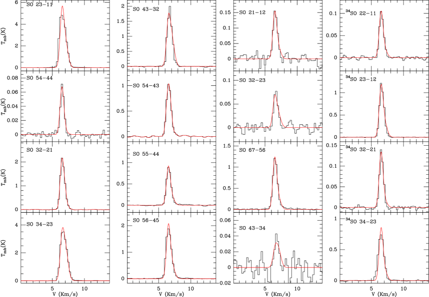
Figure 15: The same as Fig 14

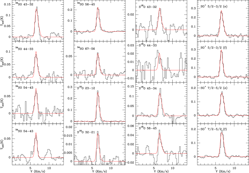
Figure 16: The same as Fig 14

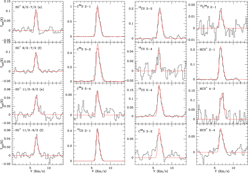
Figure 17: The same as Fig 14

Figure 18: The same as Fig 14

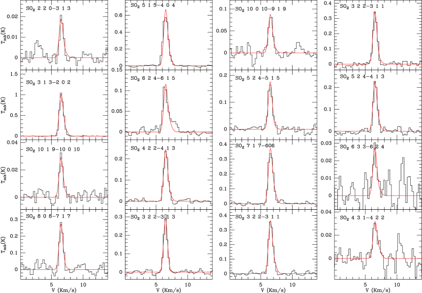
Figure 19: The same as Fig 14

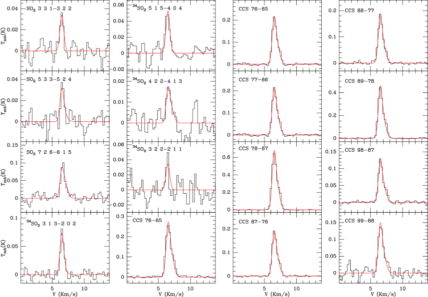
Figure 20: The same as Fig 14

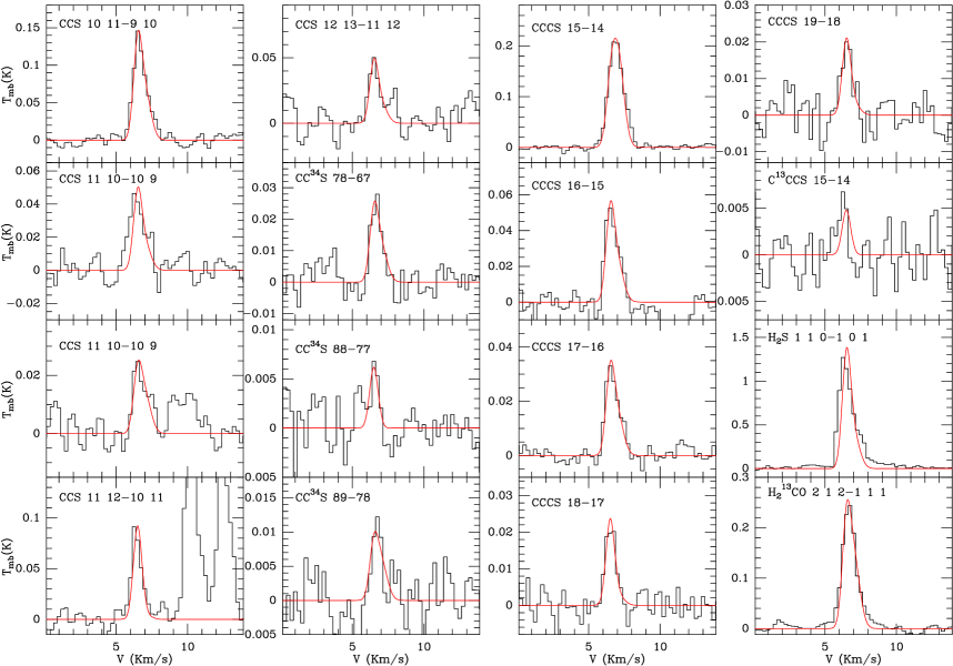
Figure 21: The same as Fig 14

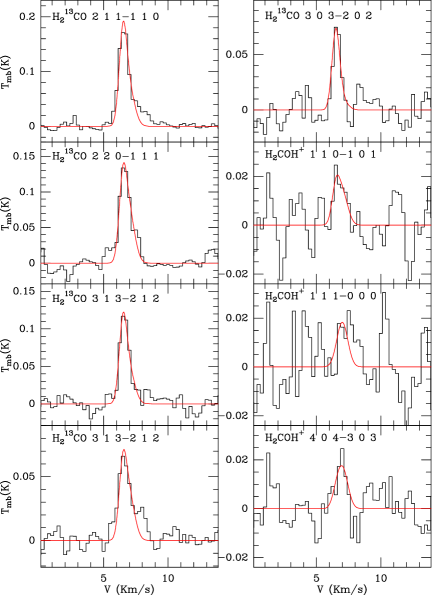
Figure 22: The same as Fig 14