Characteristics of persistent spin current components in a quasi-periodic Fibonacci ring with spin-orbit interactions: Prediction of spin-orbit coupling and on-site energy

Abstract

In the present work we investigate the behavior of all three components of persistent spin current in a quasi-periodic Fibonacci ring subjected to Rashba and Dresselhaus spin-orbit interactions. Analogous to persistent charge current in a conducting ring where electrons gain a Berry phase in presence of magnetic flux, spin Berry phase is associated during the motion of electrons in presence of a spin-orbit field which is responsible for the generation of spin current. The interplay between two spin-orbit fields along with quasi-periodic Fibonacci sequence on persistent spin current is described elaborately, and from our analysis, we can estimate the strength of any one of two spin-orbit couplings together with on-site energy, provided the other is known.

I Introduction

The study of spin dependent transport in low-dimensional quantum systems, particularly ring-like geometries, has always been intriguing due to their strange behavior and possible potential applications in designing spintronic devices. To do this proper spin regulation is highly important. Several attempts dev1 ; th1 ; th2 ; th3 ; th4 ; th5 ; th6 ; th7 ; th8 ; th9 ; th10 have been made in the last couple of decades, and undoubtedly, a wealth of literature knowledge has been established towards this direction. Mostly external magnetic fields or ferromagnetic leads were used conv1 ; conv2 to control electron spin but none of these are quite suitable from experimental perspective. This is because confining a large magnetic field in a small

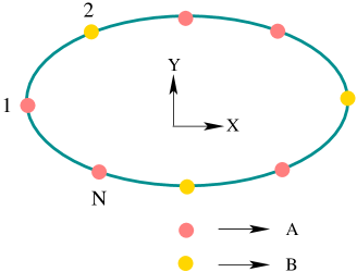
Figure 1: (Color online). Schematic view of a $8$-site mesoscopic Fibonacci ring ($5$th generation) subjected to Rashba and Dresselhaus spin-orbit interactions. The ring is constructed with two basic atomic units $A$ and $B$, and they are described by two colored filled circles.

region e.g., ring-like geometry is always a difficult task, and at the same footing major problem arises during spin injection from ferromagnetic leads through a conducting junction due to large inconsistency in resistivity. Certainly it demands new methodologies and attention has been paid towards the intrinsic properties so1 ; so2 ; so3 ; so4 ; so5 ; so6 ; so7 ; so8 ; so9 ; so10 ; n1 ; n2 like spin-orbit (SO) coupling of the materials. Usually two types of SO fields are encountered in studying spin dependent transport phenomena. One is known as Rashba SO coupling rashba which is generated due to breaking of symmetry in confining potential, and thus, can be regulated externally guo by gate electrodes. While the other, defined as Dresselhaus SO coupling dressel , is observed due to the breaking of structural symmetry. The SO field plays an essential role in spintronic applications as it directly couples to the electron’s spin degree of freedom.

In presence of such SO field a net circulating spin current is established qf1 in a conducting ring, analogous to magnetic flux driven persistent charge current ab1 ; ab2 ; ab3 . The magnetic flux introduces a phase, called Berry phase, to moving electrons which produces net charge current by breaking time reversal symmetry between clockwise and anti-clockwise moving electrons, while a spin Berry phase is associated in presence of SO coupling which generates spin current.

The works involving persistent spin current in ring-like geometries studied so far are mostly confined to the perfect periodic lattices or completely random ones ding ; AC ; san1 ; san2 . But, to the best of our knowledge, no one has addressed the behavior of SO-interaction induced spin current in quasi-periodic lattices which can bridge the gap between an ordered lattice and a fully random one. In addition, the earlier studies essentially focused on only one component (viz, $Z$-component), though it is extremely interesting and important too to study all three components of spin current to analyze spin dynamics of moving electrons in presence of SO fields. Motivated with this, in the present work we explore the behavior of persistent spin current in a one-dimensional (1D) quasi-periodic ring geometry where lattice sites are arranged in a Fibonacci sequence site1 ; site2 ; site3 , the simplest example of a quasi-periodic system. A Fibonacci chain is constructed by two basic units $A$ and $B$ following the specific rule $A\rightarrow AB$ and $B\rightarrow A$. Thus, applying successively this substitutional rule, staring from $A$ lattice or $B$ lattice we can construct the full lattice for any particular generation, say $p$-th generation, obeying the prescription $F_{p}=F_{p-1}\otimes F_{p-2}$, and connecting its two ends we get the required ring model. Thus, if we start with $A$ lattice then $A$, $AB$, $ABA$, $ABAAB$, $ABAABABA$, $\dots$, etc., are the first few generations, and the series is characterized by the ratio of total number of $A$ and $B$ atoms which is called as Golden mean $\tau$ ($=1+\sqrt{5}/2$). Now, instead of considering $A$ and $B$ as lattice points if we assign them as bond variables then bond model of Fibonacci generation is established bond1 ; bond2 , and when both these lattice and bond models are taken into account it becomes a mixed model site2 . In our model we consider only site representation of Fibonacci sequence starting with lattice $A$, for the sake of simplification. The response of other will be discussed elsewhere in our future work.

In this work, we address the behavior of all three components of persistent spin current in a Fibonacci ring subjected to Rashba and Dresselhaus SO couplings. Within a tight-binding framework we calculate the current components using second-quantized approach which is the most convenient tool for such calculations. The interplay between Rashba and Dresselhaus SO fields on the current components exhibits several interesting patterns that can be utilized to estimate any one of the SO fields if we know the other one, and also we can estimate the site energy of $A$- or $B$-type site provided any one of these two is given. Our analysis can be utilized to explore spin dependent phenomena in any correlated lattices subjected to such kind of SO fields. This is the first step towards this direction.

The work is arranged as follows. In Sec. II we present the model and theoretical framework for calculations. The results are discussed in Sec. III, and finally we conclude in Sec. IV.

II Model and Theoretical Formulation

The mesoscopic Fibonacci ring subjected to Rashba and Dresselhaus SO couplings is schematically depicted in Fig. 1, and the Hamiltonian of such a ring reads as,

$$\mbox{\boldmath$H$}=\mbox{\boldmath$H$}_{\mbox{\tiny 0}}+\mbox{\boldmath$H$}_{\mbox{\tiny R}}+\mbox{\boldmath$H$}_{\mbox{\tiny D}}$$ (1)

which includes the SO-coupled free term ($\mbox{\boldmath$H$}_{\mbox{\tiny 0}}$), Rashba Hamiltonian ($\mbox{\boldmath$H$}_{\mbox{\tiny R}}$) and the Dresselhaus Hamiltonian ($\mbox{\boldmath$H$}_{\mbox{\tiny D}}$). Using tight-binding (TB) framework we can express these Hamiltonians site3 for a $N$-site ring as follows:

$$\mbox{\boldmath$H$}_{\mbox{\tiny 0}} = \sum\limits_{n}\mbox{\boldmath$c$}_{n}^{\dagger}\mbox{\boldmath$\epsilon$}_{n}\mbox{\boldmath$c$}_{n}+\sum\limits_{n}\left(\mbox{\boldmath$c$}_{n+1}^{\dagger}\mbox{\boldmath$t$}\mbox{\boldmath$c$}_{n}+\mbox{\boldmath$c$}_{n}^{\dagger}\mbox{\boldmath$t$}\mbox{\boldmath$c$}_{n+1}\right)$$ (2a)

$$\mbox{\boldmath$H$}_{\mbox{\tiny R}} = -\sum\limits_{n}\left(\mbox{\boldmath$c$}_{n+1}^{\dagger}\left(i\mbox{\boldmath$\sigma$}_{x}\right)\mbox{\boldmath$\alpha$}\cos\phi_{n,n+1}\mbox{\boldmath$c$}_{n}+h.c.\right)$$

$$-\sum\limits_{n}\left(\mbox{\boldmath$c$}_{n+1}^{\dagger}\left(i\mbox{\boldmath$\sigma$}_{y}\right)\mbox{\boldmath$\alpha$}\sin\phi_{n,n+1}\mbox{\boldmath$c$}_{n}+h.c.\right)$$ (2b)

$$\mbox{\boldmath$H$}_{\mbox{\tiny D}} = \sum\limits_{n}\left(\mbox{\boldmath$c$}_{n+1}^{\dagger}\left(i\mbox{\boldmath$\sigma$}_{y}\right)\mbox{\boldmath$\beta$}\cos\phi_{n,n+1}\mbox{\boldmath$c$}_{n}+h.c.\right)$$

$$+\sum\limits_{n}\left(\mbox{\boldmath$c$}_{n+1}^{\dagger}\left(i\mbox{\boldmath$\sigma$}_{x}\right)\mbox{\boldmath$\beta$}\sin\phi_{n,n+1}\textbf{c}_{n}+h.c.\right)$$ (2c)

where the site index $n$ runs from $1$ to $N$, and we use the condition $N+1=1$. The other factors are: $\mbox{\boldmath$\epsilon$}_{n}=\left(\begin{array}[]{cc}\epsilon_{n\uparrow}&0\\ 0&\epsilon_{n\downarrow}\end{array}\right)$, $\mbox{\boldmath$t$}=\left(\begin{array}[]{cc}t&0\\ 0&t\end{array}\right)$, $\mbox{\boldmath$c$}_{n}=\left(\begin{array}[]{cc}c_{n\uparrow}\\ c_{n\downarrow}\end{array}\right)$, $\mbox{\boldmath$\alpha$}=\left(\begin{array}[]{cc}\alpha&0\\ 0&\alpha\end{array}\right)$, $\mbox{\boldmath$\beta$}=\left(\begin{array}[]{cc}\beta&0\\ 0&\beta\end{array}\right)$ where $t$ is the nearest-neighbor hopping integral and $\epsilon_{n\uparrow}$ ($\epsilon_{n\downarrow}$) represents the on-site energy of an up (down) spin electron sitting at the $n$th site. As we are not considering any magnetic type interaction the site energies for up and down spin electrons become equal i.e., $\epsilon_{n\uparrow}=\epsilon_{n\downarrow}=\epsilon_{n}$ (say). For the $A$-type sites we refer $\epsilon_{n}=\epsilon_{A}$, and similarly, $\epsilon_{n}=\epsilon_{B}$ for $B$-type atomic sites. When these two site energies are identical (viz, $\epsilon_{A}=\epsilon_{B}$) the Fibonacci ring becomes a perfect one, and in that case we set them to zero without loss of any generality. $\alpha$ and $\beta$ are the Rashba and Dresselhaus SO coupling strengths, respectively, and $\phi_{n,n+1}=\left(\phi_{n}+\phi_{n+1}\right)/2,$ where $\phi_{n}=2\pi(n-1)/N$. $\mbox{\boldmath$\sigma$}_{i}$’s ($i=x$, $y$, $z$) are the Pauli spin matrices in $\mbox{\boldmath$\sigma$}_{z}$ diagonal representation.

Looking carefully the Rashba and Dresselhaus Hamiltonians (Eqs. 2(b) and 2(c)) one can find that these two Hamiltonians are connected by a unitary transformation $\mbox{\boldmath$H$}_{\mbox{\tiny D}}=\mbox{\boldmath$U$}\mbox{\boldmath$H$}_{\mbox{\tiny R}}\mbox{\boldmath$U$}^{\dagger}$, where $\mbox{\boldmath$U$}=\mbox{\boldmath$\sigma$}_{z}(\mbox{\boldmath$\sigma$}_{x}+\mbox{\boldmath$\sigma$}_{y})/\sqrt{2}$. This hidden transformation relation leads to several interesting results, in particular when the strengths of these two SO couplings are equal, which will be available in our next section (Sec. III).

To calculate spin current components we define the operator ding $\mbox{\boldmath$I$}_{k}=\frac{1}{2N}\left(\mbox{\boldmath$\sigma$}_{k}\dot{\mbox{\boldmath$x$}}+\dot{\mbox{\boldmath$x$}}\mbox{\boldmath$\sigma$}_{k}\right)$, where $k=x$, $y$, $z$ depending on the specific component. In this expression $\dot{\mbox{\boldmath$x$}}$ is obtained by taking the commutation of position operator $x$ ($=\sum\limits_{n}\mbox{\boldmath$C$}_{n}^{\dagger}n\mbox{\boldmath$C$}_{n}$) with the Hamiltonian $H$. After simplification the current operator gets the form:

$$\mbox{\boldmath$I$}_{k} = \frac{i\pi}{N}\sum\limits_{n}\left(\mbox{\boldmath$c$}_{n}^{\dagger}\mbox{\boldmath$\sigma$}_{k}\mbox{\boldmath$t$}_{\phi}^{\dagger n,n+1}\mbox{\boldmath$c$}_{n+1}-h.c.\right)$$ (3)

$$+\frac{i\pi}{N}\sum\limits_{n}\left(\mbox{\boldmath$c$}_{n}^{\dagger}\mbox{\boldmath$t$}_{\phi}^{\dagger n,n+1}\mbox{\boldmath$\sigma$}_{k}\mbox{\boldmath$c$}_{n+1}-h.c.\right)$$

where, $\mbox{\boldmath$t$}_{\phi}^{n,n+1}$ is a ($2\times 2$) matrix whose elements are ${\mbox{\boldmath$t$}_{\phi}^{n,n+1}}_{1,1}=t$ ${\mbox{\boldmath$t$}_{\phi}^{n,n+1}}_{2,2}=t$ ${\mbox{\boldmath$t$}_{\phi}^{n,n+1}}_{1,2}=-i\alpha e^{-i\phi_{n,n+1}}+\beta e^{i\phi_{n,n+1}}$ ${\mbox{\boldmath$t$}_{\phi}^{n,n+1}}_{2,1}=-i\alpha e^{i\phi_{n,n+1}}-\beta e^{i\phi_{n,n+1}}$. Once the current operator is established (Eq. 3), the individual current components carried by each eigenstate, say $|\psi_{m}\rangle$, can be easily found from the operation $I_{k,m}=\langle\psi_{m}|\mbox{\boldmath$I$}_{k}|\psi_{m}\rangle$, where $|\psi_{m}\rangle=\sum\limits_{n}\left(a_{n\uparrow}^{m}|n\uparrow\rangle+a_{n\downarrow}^{m}|n\downarrow\rangle\right)$. $a_{n\sigma}^{m}$’s are the coefficients. Doing a quite long and straightforward calculation we eventually get the following current expressions for three different directions ($X$, $Y$ and $Z$) as follows:

$$I_{z,m} = \frac{2\pi it}{N}\sum\limits_{n}\left[\left\{a_{n,\uparrow}^{m\ast}a_{n+1,\uparrow}^{m}-h.c.\right\}-\left\{a_{n,\downarrow}^{m\ast}a_{n+1,\downarrow}^{m}-\right.\right.$$

$$\left.\left.h.c.\right\}\right]$$ (4a)

$$I_{x,m} = \frac{2\pi it}{N}\sum\limits_{n}\left\{\left(a_{n,\uparrow}^{m\ast}a_{n+1,\downarrow}^{m}+a_{n,\downarrow}^{m\ast}a_{n+1,\uparrow}^{m}\right)-h.c.\right\}$$

$$+\frac{2\pi}{N}\sum\limits_{n}\left\{\left(a_{n+1,\uparrow}^{m\ast}a_{n,\uparrow}^{m}+a_{n+1,\downarrow}^{m\ast}a_{n,\downarrow}^{m}\right)+h.c.\right\}\times$$

$$\left(\beta\sin\phi_{n,n+1}-\alpha\cos\phi_{n,n+1}\right)$$ (4b)

$$I_{y,m} = \frac{2\pi t}{N}\sum\limits_{n}\left\{\left(a_{n+1,\downarrow}^{m\ast}a_{n,\uparrow}^{m}-a_{n+1,\uparrow}^{m\ast}a_{n,\downarrow}^{m}\right)+h.c.\right\}$$

$$+\frac{2\pi}{N}\sum\limits_{n}\left\{\left(a_{n+1,\uparrow}^{m\ast}a_{n,\uparrow}^{m}+a_{n+1,\downarrow}^{m\ast}a_{n,\downarrow}^{m}\right)+h.c.\right\}\times$$

$$\left(\beta\cos\phi_{n,n+1}-\alpha\sin\phi_{n,n+1}\right)$$ (4c)

Thus, at absolute zero temperature, the net current for a $N_{e}$ electron system becomes

$$I_{k}=\sum\limits_{m=1}^{N_{e}}I_{k,m}.$$ (5)

III Results

Based on the above theoretical framework now we present our numerical results which include three different current components carried by individual energy eigenstates, net currents of all three components for a particular electron filling $N_{e}$, and the possibilities of determining any one of the SO fields as well as on-site energies provided the other is known. As we are not focusing on quantitative analysis considering a particular material, we choose $c=e=h=1$ for the sake of simplification and fix the nearest-neighbor hopping integral $t=1.5$ throughout the analysis. The values of other parameters are given in subsequent figures.

III.1 Current components carried by distinct energy levels

Before analyzing net current components for a specific filling factor, let us first focus on the behavior of individual state currents as they give more clear conducting signature of separate energy levels which essentially govern the net response of any system.

In Fig. 2 we present the variation of $Z$-component of spin current carried by individual energy levels for a completely perfect (left column) and a Fibonacci ring (right column) in presence of different

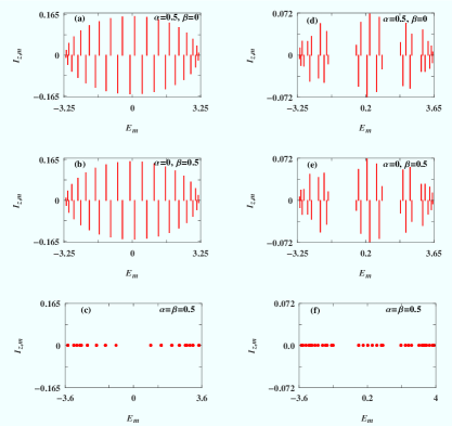
Figure 2: (Color online). $Z$-component of spin current ($I_{z,m}$) carried by individual energy levels (levels are indexed by the parameter $m$ and $E_{m}$ being the energy eigenvalue of $m$th level) for $34$-site ring ($8$th generation) considering different values of $\alpha$ and $\beta$, where the first and second columns correspond to $\epsilon_{A}=\epsilon_{B}=0$ and $\epsilon_{A}=-\epsilon_{B}=1$, respectively.

SO couplings. Several interesting features are observed. (i) In presence of any one of the two SO fields individual state currents exhibit a nice pattern for the perfect case where the current starts increasing (each vertical line represents the current amplitude for each state) from the energy band edge and reaches to a maximum at the band centre. While, for the Fibonacci ring sub-spectra with finite gaps, associated with energy sub-bands, are obtained which is the generic feature of any Fibonacci lattice, like other quasi-crystals g1 ; g2 . In each sub-band higher currents are obtained from central energy levels while edge states provide lesser currents, similar to a perfect ring. Thus, setting the Fermi energy, associated with electron filling $N_{e}$, at the centre or towards the edge of each sub-band one can regulate current amplitude and this phenomenon can be visualized at multiple energies due to the appearance of multiple energy sub-bands. Here it is also crucial to note that no such phenomenon will be observed in a completely random disordered ring as it exhibits only localized states for the entire energy band region. (ii) Successive energy levels carry currents in opposite directions which gives an important conclusion that the net $Z$-component of current is controlled basically by the top most filled energy level, similar to that what we get in the case of conventional magnetic flux induced persistent charge current in a conducting mesoscopic ring. (iii) Finally, it is important to see that the direction of individual state currents in a ring subjected to only Rashba SO coupling gets exactly reversed when the ring is described with only Dresselhaus SO interaction, without changing any magnitude. Thus, if both these two SO fields are present in a particular sample and if they are equal in magnitude then current carried by different eigenstates drops exactly to zero due to mutual cancellation of current caused by these fields. This vanishing nature of spin current can be proved as follows. It is already pointed out that $\mbox{\boldmath$H$}_{\mbox{\tiny R}}$ and $\mbox{\boldmath$H$}_{\mbox{\tiny D}}$ are connected by a unitary transformation $\mbox{\boldmath$H$}_{\mbox{\tiny D}}=\mbox{\boldmath$U$}\mbox{\boldmath$H$}_{\mbox{\tiny R}}\mbox{\boldmath$U$}^{\dagger}$. Therefore, if $|\psi_{m}\rangle$ be an eigenstate of $\mbox{\boldmath$H$}_{\mbox{\tiny R}}$ then $\mbox{\boldmath$U$}|\psi_{m}\rangle$ ($=|\psi_{m}^{\prime}\rangle$) will be the eigenstate of the Hamiltonian $\mbox{\boldmath$H$}_{\mbox{\tiny D}}$. This immediately gives us the following relation:

$$I_{z,m}|_{\mbox{\tiny D}} = \langle\psi_{m}^{\prime}|\mbox{\boldmath$I$}_{z,m}|\psi_{m}^{\prime}\rangle$$ (6)

$$= \langle\psi_{m}|\mbox{\boldmath$U$}^{\dagger}\mbox{\boldmath$I$}_{z,m}\mbox{\boldmath$U$}|\psi_{m}\rangle$$

$$= \langle\psi_{m}|\mbox{\boldmath$U$}^{\dagger}\frac{1}{2N}\left(\mbox{\boldmath$\sigma$}_{z}\dot{\mbox{\boldmath$x$}}+\dot{\mbox{\boldmath$x$}}\mbox{\boldmath$\sigma$}_{z}\right)\mbox{\boldmath$U$}|\psi_{m}\rangle$$

$$= \langle\psi_{m}|\frac{1}{2N}\left(-\mbox{\boldmath$\sigma$}_{z}\dot{\mbox{\boldmath$x$}}-\dot{\mbox{\boldmath$x$}}\mbox{\boldmath$\sigma$}_{z}\right)|\psi_{m}\rangle$$

$$= -I_{z,m}|_{\mbox{\tiny R}}$$

From the above mathematical argument the sign reversal of $I_{z,m}$ under interchanging the roles played by $\alpha$ and $\beta$ can be easily understood. Certainly this vanishing behavior can be exploited to determine any one among these two SO fields if the other is given. In particular the determination of Dresselhaus strength will be much easier as for a specific material it is constant, while Rashba strength can be tuned with the help of external gate potential. Here, it is worthy to note that the interplay of Rashba and Dresselhaus SO couplings has also been reported in several other contexts, and particularly when these two strengths are equal, persistent spin helix sh1 ; sh2 ; sh3 ; sh4 has observed which is of course one of the most important and attractive areas of spintronics.

In Figs. 3 and 4 we present the characteristics of $X$ and $Y$ components of spin current, respectively, carried by individual energy levels for the identical ring size and parameter values as taken in Fig. 2 for finer comparison of all three components. The observations are noteworthy. (i) For the perfect ring (viz, $\epsilon_{A}=\epsilon_{B}=0$), both $X$ and $Y$ components of current are zero for each energy eigenstates, while non-zero contribution comes from the Fibonacci ring. In order to explain this behavior let us focus on Fig. 5, where the velocity direction of a moving electron is schematically shown at different lattice points of a ring placed in the $X$-$Y$ plane. Now, consider the Rashba and Dresselhaus Hamiltonians in a continuum representation where they get the forms: $\mbox{\boldmath$H$}_{\mbox{\tiny R}}=\alpha\left(\mbox{\boldmath$\sigma$}_{y}\mbox{\boldmath$p$}_{x}-\mbox{\boldmath$\sigma$}_{x}\mbox{\boldmath$p$}_{y}\right)$ and $\mbox{\boldmath$H$}_{\mbox{\tiny D}}=\beta\left(\mbox{\boldmath$\sigma$}_{y}\mbox{\boldmath$p$}_{y}-\mbox{\boldmath$\sigma$}_{x}\mbox{\boldmath$p$}_{x}\right)$ where $\mbox{\boldmath$p$}_{x}$ and $\mbox{\boldmath$p$}_{y}$ are the components of $p$ along $X$ and $Y$ directions, respectively. Thus, at the point A of a pure Rashba ring

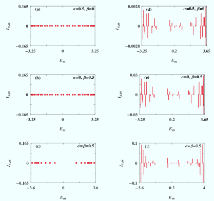
Figure 3: (Color online). $X$-component of spin current ($I_{x,m}$) carried by distinct energy levels of a mesoscopic ring where different spectra correspond to the identical meanings as described in Fig. 2. The ring size and other physical parameters are also same as taken in Fig. 2.

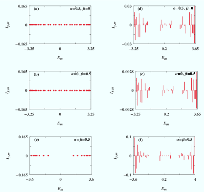
Figure 4: (Color online). $Y$-component of persistent spin current ($I_{y,m}$) for separate energy levels of a conducting ring in presence of $\alpha$ and $\beta$, where the different spectra represent the similar meanings as described in Fig. 2. The physical parameters remain unchanged as taken in Fig. 2.

only $\mbox{\boldmath$p$}_{y}$ will contribute (since here $\mbox{\boldmath$p$}_{x}=0$) to $\mbox{\boldmath$H$}_{\mbox{\tiny R}}$, while it is $-\mbox{\boldmath$p$}_{y}$ at the point C (Fig. 5). Similarly, for the points B and D the contributing terms are $\mbox{\boldmath$p$}_{x}$ and $-\mbox{\boldmath$p$}_{x}$, respectively. As a result of this the net contribution to $\mbox{\boldmath$H$}_{\mbox{\tiny R}}$ becomes zero, and this is equally true for any other diagonally opposite points (though in these cases both $\mbox{\boldmath$p$}_{x}$ and $\mbox{\boldmath$p$}_{y}$ contribute) which leads to a vanishing spin current along $X$ and $Y$ directions for a perfect Rashba ring. The same argument is also valid in the case of a pure Dresselhaus

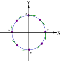
Figure 5: (Color online). Velocity direction (green arrow) of a moving electron at some typical points (filled colored circles) of a ring placed in the $X$-$Y$ plane.

ring. But, as long as the symmetry between the diagonally opposite points is broken the mutual cancellation does not take place which results a finite non-zero spin current along these two directions. This is exactly what we get in a Fibonacci ring, and in the same footing, we can expect non-zero spin current for any other disordered rings. (ii) In the Fibonacci ring the $X$-component ($Y$-component) of spin current in presence of $\alpha$ maps exactly in the opposite sense (i.e., identical magnitude but opposite in direction) to the $Y$-component ($X$-component) of current under swapping the roles played by $\alpha$ and $\beta$ (right columns of Figs. 3 and 4). This phenomenon can be explained from the following mathematical analysis.

$$I_{y,m}|_{\mbox{\tiny D}} = \langle\psi^{\prime}_{m}|\mbox{\boldmath$I$}_{y,m}|\psi^{\prime}_{m}\rangle$$ (7)

$$= \langle\psi_{m}|\mbox{\boldmath$U$}^{\dagger}\mbox{\boldmath$I$}_{y,m}\mbox{\boldmath$U$}|\psi_{m}\rangle$$

$$= \langle\psi_{m}|\mbox{\boldmath$U$}^{\dagger}\frac{1}{2N}\left(\mbox{\boldmath$\sigma$}_{y}\dot{\mbox{\boldmath$x$}}+\dot{\mbox{\boldmath$x$}}\mbox{\boldmath$\sigma$}_{y}\right)\mbox{\boldmath$U$}|\psi_{m}\rangle$$

$$= \langle\psi_{m}|\frac{1}{2N}\left(-\mbox{\boldmath$\sigma$}_{x}\dot{\mbox{\boldmath$x$}}-\dot{\mbox{\boldmath$x$}}\mbox{\boldmath$\sigma$}_{x}\right)|\psi_{m}\rangle$$

$$= -I_{x,m}|_{\mbox{\tiny R}}$$

and

$$I_{x,m}|_{\mbox{\tiny D}} = \langle\psi^{\prime}_{m}|\mbox{\boldmath$I$}_{x,m}|\psi^{\prime}_{m}\rangle$$ (8)

$$= \langle\psi_{m}|\mbox{\boldmath$U$}^{\dagger}\mbox{\boldmath$I$}_{x,m}\mbox{\boldmath$U$}|\psi_{m}\rangle$$

$$= \langle\psi_{p}|\mbox{\boldmath$U$}^{\dagger}\frac{1}{2N}\left(\mbox{\boldmath$\sigma$}_{x}\dot{\mbox{\boldmath$x$}}+\dot{\mbox{\boldmath$x$}}\mbox{\boldmath$\sigma$}_{x}\right)\mbox{\boldmath$U$}|\psi_{m}\rangle$$

$$= \langle\psi_{m}|\frac{1}{2N}\left(-\mbox{\boldmath$\sigma$}_{y}\dot{\mbox{\boldmath$x$}}-\dot{\mbox{\boldmath$x$}}\mbox{\boldmath$\sigma$}_{y}\right)|\psi_{m}\rangle$$

$$= -I_{y,m}|_{\mbox{\tiny R}}$$

Equations 7 and 8 clearly describe the interchange of $X$ and $Y$ components of current under the reciprocation of $\alpha$ and $\beta$. (iii) Quite interestingly we see that both for these two components ($X$ and $Y$) the states lying towards the energy band edge carry higher current compared to the inner states, unlike the $Z$-component of current where opposite signature is noticed. This feature is also observed in other quasi-periodic rings as well as in a fully random one. In addition, a significant change in current amplitude takes place between the two current components when the ring is subjected to either $\alpha$ or $\beta$, even if these strengths are identical (Figs. 3(d) and (e); (Figs. 4(d) and (e)), though its proper physical explanation is not clear to us. (iv) Finally, it is important to note that at $\alpha=\beta$ none of these $X$ and $Y$ components of current vanishes (see Figs. 3(f) and 4(f)) since $I_{y,m}|_{\mbox{\tiny D}}\neq-I_{y,m}|_{\mbox{\tiny R}}$ and also $I_{x,m}|_{\mbox{\tiny D}}\neq-I_{x,m}|_{\mbox{\tiny R}}$.

III.2 Components of net current for a particular electron filling

Now we focus on the behavior of all three components of spin current for a particular electron filling and the total spin current taking the contributions from these individual components.

In Fig. 6 we present the variation of $Z$-component of spin

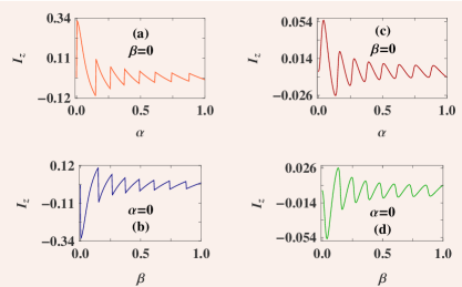
Figure 6: (Color online). $Z$-component of spin current ($I_{z}$) as a function of any one of two SO fields (keeping the other at zero) for a $89$-site ring ($10$th generation) considering $N_{e}=50$, where the left and right columns correspond to $\epsilon_{A}=\epsilon_{B}=0$ and $\epsilon_{A}=-\epsilon_{B}=1$, respectively.

current as a function of SO coupling for a $89$-site ring considering $N_{e}=50$. In the first column the results are shown for a perfect ring, while for the Fibonacci ring they are presented in the other column. The current exhibits an anomalous oscillation with SO coupling and its amplitude gradually decreases with increasing the coupling strength. This oscillation is characterized by the crossing of different distinct energy levels (viz, degeneracy) of the system, and also observed in other context san1 ; site3 . The other feature i.e., the phase reversal of $I_{z}$ by interchanging the parameters $\alpha$ and $\beta$ can be well understood from our

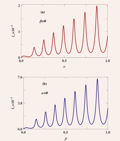
Figure 7: (Color online). $X$-component of spin current ($I_{x}$) as a function of any one of the two SO interactions for a $89$-site ($10$th generation) Fibonacci ring ($\epsilon_{A}=-\epsilon_{B}=1$) considering $N_{e}=50$.

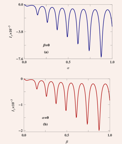
Figure 8: (Color online). $Y$-component of spin current ($I_{y}$) as a function of any one of the two SO interactions for a $89$-site ($10$th generation) Fibonacci ring ($\epsilon_{A}=-\epsilon_{B}=1$) considering $N_{e}=50$.

previous analysis, and thus, the net $Z$-component of spin current should vanish under the situation $\alpha=\beta$, which is not shown here to save space. In addition, it is also observed that the net current amplitude in the Fibonacci ring (right column of Fig. 6) for any $\alpha$ or $\beta$ is much smaller than the perfect one (left column of Fig. 6), and it is solely associated with the conducting nature of different energy levels those are contributing to the current. The nature of current carrying states can be clearly noticed from the spectra given in Fig. 2, where the currents carried by distinct energy levels of the Fibonacci ring are much smaller compared to the perfect one.

The behaviors of other two current components (viz, $X$ and $Y$) are shown in Figs. 7 and 8. Since both these two components are zero for the perfect ring, here we present the results only for a Fibonacci ring considering the identical parameter values and electron filling as taken in Fig. 6. The current exhibits an oscillation, and unlike $Z$-component, the oscillating peak increases with increasing SO interaction.

Finally, focus on the spectra shown in Fig. 9 where we present the variation of net spin current $I_{s}$ taking the individual contributions from three different components. It is defined as

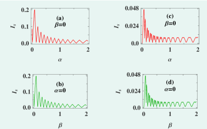
Figure 9: (Color online). Net spin current $I_{s}$ (considering the contributions from all three components) as a function of any one of two SO interactions (setting the other at zero) for a $89$-site ($10$th generation) ring with $50$ electrons, where the first and second columns correspond to $\epsilon_{A}=\epsilon_{B}=0$ and $\epsilon_{A}=-\epsilon_{B}=1$, respectively.

$I_{s}=\sqrt{I_{x}^{2}+I_{y}^{2}+I_{z}^{2}}$. Both the perfect and Fibonacci rings are taken into account those are placed in the first and second columns of Fig. 9, respectively. In both these two cases we find oscillating behavior of current following the current components as discussed in Figs. 6-8. For the ordered ring since the contribution comes only from $I_{z}$, the oscillation of $I_{s}$ gradually dies out with SO coupling. While for the Fibonacci ring as $I_{x}$ and $I_{y}$ along with $I_{z}$ contribute to $I_{s}$, a finite but small oscillation still persists even for higher values of SO coupling. The another feature obtained from the spectra i.e., lesser $I_{s}$ in Fibonacci ring compared to the perfect one for any non-zero SO coupling is quite obvious.

III.3 Prediction of on-site energy

In this sub-section we discuss the possibilities of estimating any one of the two on-site potentials ($\epsilon_{A}$ and $\epsilon_{B}$) of a Fibonacci ring if we known the other one.

This can be done quite easily by analyzing the behavior of current amplitude of individual components as a function of either $\epsilon_{A}$ or $\epsilon_{B}$, setting the other constant, keeping in mind that a distinct feature may appear when these two site energies become identical since the current components are significantly influenced by the disorderness.

In Fig. 10 we show the variation of $I_{z}$ as a function of

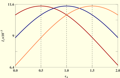
Figure 10: (Color online). $I_{z}$ vs. $\epsilon_{A}$ for a $55$-site ($9$th generation) Fibonacci ring for three distinct values of $\epsilon_{B}$, where the red, navy and orange curves correspond to $\epsilon_{B}=0.5$, $1$ and $1.5$, respectively. The other physical parameters are: $N_{e}=55$, $\alpha=1$ and $\beta=0$.

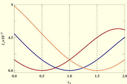
Figure 11: (Color online). Same as Fig. 10 where the variation of $I_{x}$ with $\epsilon_{A}$ is shown.

$\epsilon_{A}$ for a $55$-site Fibonacci ring with $55$ electrons considering three distinct values of $\epsilon_{B}$ those are represented by three different colored curves. Here we take $\alpha=1$ and fix $\beta$ to zero. Interestingly we see that $I_{z}$ reaches to the maximum (shown by the dotted line) when the two site energies are equal. While, the current amplitude gets reduced with increasing the deviation of site energies i.e., $|\epsilon_{A}-\epsilon_{B}|$. This is solely associated with localizing behavior of electronic waves and directly linked with previous analysis. Thus, for a particular material composed of two different lattices one can determine the site energy of any one by varying the other and observing the maximum of $I_{z}$. It takes place only when $\epsilon_{A}=\epsilon_{B}$.

In the same footing, we can also find a definite condition from the other two current components through which site energy is predicted. The results

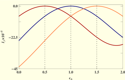
Figure 12: (Color online). Same as Fig. 10 where the variation of $I_{y}$ with $\epsilon_{A}$ is shown.

are presented in Figs. 11 and 12 for the identical ring and parameter values as taken in Fig. 10. From these spectra it is clearly seen that when $\epsilon_{A}$ becomes equal to $\epsilon_{B}$, both $X$ and $Y$ components of spin current drop exactly zero, and this vanishing behavior leads to the possibility of determining site energy.

Before we end this sub-section it is important to note that from the practical point of view one may think how site energies of a large number of $A$-type or $B$-type sites can be tuned for large sized ring. This is of course a difficult task. But, through the present analysis we intend to establish that if we take a ring geometry with few foreign atoms, then this prescription will be useful since tuning the site energies of only these few atoms by means of external gate potential site energies of parent atoms can be estimated.

IV Summary and conclusions

In summary, we have made a comprehensive analysis of all three components of persistent spin current in a quasi-periodic Fibonacci ring with Rashba and Dresselhaus SO interactions. Within a tight-binding framework we compute all the current components based on second-quantized approach. Several distinct features have been observed those can be utilized to determine any one of the two SO fields as well as the site energies when the other is known.

The results studied in this work are for a generic model, not related to any specific material, and thus, can be extended to any such correlated as well as uncorrelated lattice models and can provide some basic inputs towards spin dependent transport phenomena.

V Acknowledgment

MP is thankful to University Grants Commission (UGC), India for research fellowship.

References

- (1) S. A. Wolf, D. D. Awschalom, R. A. Buhrman, J. M. Daughton, S. von Molnár, M. L. Roukes, A. Y. Chtchelkanova, and D. M. Treger, Science 294, 1488 (2001).
- (2) I. Zutic, J. Fabian, and S. Das Sarma, Rev. Mod. Phys. 76, 323 (2004).
- (3) S. Datta and B. Das, Appl. Phys. Lett. 56, 665 (1990).
- (4) S. Bellucci and P. Onorato, Phys. Rev. B 78, 235312 (2008).
- (5) P. Földi, B. Molnár, M. G. Benedict, and F. M. Peeters, Phys. Rev. B 71, 033309 (2005).
- (6) P. Földi, M. G. Benedict, O. Kálmán, and F. M. Peeters, Phys. Rev. B 80, 165303 (2009).
- (7) S. Bellucci and P. Onorato, J. Phys.: Condens. Matter 19, 395020 (2007).
- (8) S.-Q. Shen, Z.-J. Li, and Z. Ma, Appl. Phys. Lett. 84, 996 (2004).
- (9) D. Frustaglia and K. Richter, Phys. Rev. B 69, 235310 (2004).
- (10) D. Frustaglia, M. Hentschel, and K. Richter, Phys. Rev. Lett. 87, 256602 (2001).
- (11) M. Hentschel, H. Schomerus, D. Frustaglia, and K. Richter, Phys. Rev. B 69, 155326 (2004).
- (12) W. Long, Q. F. Sun, H. Guo, and J. Wang, Appl. Phys. Lett. 83, 1397 (2003).
- (13) P. Zhang, Q. K. Xue, and X. C. Xie, Phys. Rev. Lett. 91, 196602 (2003).
- (14) Q. F. Sun and X. C. Xie, Phys. Rev. B 91, 235301 (2006).
- (15) Q. F. Sun and X. C. Xie, Phys. Rev. B 71, 155321 (2005).
- (16) F. Chi, J. Zheng, and L. L. Sun, Appl. Phys. Lett. 92, 172104 (2008).
- (17) T. P. Pareek, Phys. Rev. Lett. 92, 076601 (2004).
- (18) W. J. Gong, Y. S. Zheng, and T. Q. Lü, Appl. Phys. Lett. 92, 042104 (2008).
- (19) H. F. Lü and Y. Guo, Appl. Phys. Lett. 91, 092128 (2007).
- (20) M. C. Chang, Phys. Rev. B 71, 085315 (2005).
- (21) W. Yang and K. Chang, Phys. Rev. B 73, 045303 (2006).
- (22) M. Wang and K. Chang, Phys. Rev. B 77, 125330 (2008).
- (23) M. Dey, S. K. Maiti, and S. N. Karmakar, J. Appl. Phys. 109, 024304 (2011).
- (24) N. Hatano, R. Shirasaki, and H. Nakamura, Phys. Rev. A 75, 032107 (2007).
- (25) J. Chen, M. B. A. Jalil, and S. G. Tan, J. Appl. Phys. 109, 07C722 (2011).
- (26) Y. A. Bychkov and E. I. Rashba, JETP Lett. 39, 78 (1984).
- (27) T. W. Chen, C. M. Huang, and G. Y. Guo, Phys. Rev. B 73, 235309 (2006).
- (28) G. Dresselhaus, Phys. Rev. 100, 580 (1955).
- (29) Q.-f. Sun, X. C. Xie, and J. Wang, Phys. Rev. Lett. 98, 196801 (2007).
- (30) M. Büttiker, Y. Imry, and R. Landauer, Phys. Lett. 96A, 365 (1983).
- (31) H. F. Cheung, Y. Gefen, E. K. Riedel, and W. H. Shih, Phys. Rev. B 37, 6050 (1988).
- (32) B. L. Altshuler, Y. Gefen, and Y. Imry, Phys. Rev. Lett. 66, 88 (1991).
- (33) G. H. Ding and B. Dong, Phys. Rev. B 76, 125301 (2007).
- (34) L. G. Wang and Y. L. Huang, Superlattices and Microstructures 66, 148 (2014).
- (35) S. K. Maiti, J. Appl. Phys. 110, 064306 (2011).
- (36) S. K. Maiti, M. Dey, and S. N. Karmakar, Physica E 64, 169 (2014).
- (37) X. F. Hu, R. W. Peng, L. S. Cao, X. Q. Huang, M. Wang, A. Hu, and S. S. Jiang, J. Appl. Phys. 97, 10B308 (2005).
- (38) G. J. Jin, Z. D. Wang, A. Hu, and S. S. Jiang, Phys. Rev. B 55, 9302 (1997).
- (39) M. Patra and S. K. Maiti, Eur. Phys. J. B 89, 88 (2016).
- (40) S. N. Karmakar, A. Chakrabarti, and R. K. Moitra, Phys. Rev. B 46, 3660 (1992).
- (41) R. K. Moitra, A. Chakrabarti, and S. N. Karmakar, Phys. Rev. B 66, 064212 (2002).
- (42) A.-M. Guo, Phys. Rev. E 75, 061915 (2007).
- (43) H. Lei, J. Chen, G. Nouet, S. Feng, Q. Gong, and X. Jiang, Phys. Rev. B 75, 205109 (2007).
- (44) B. A. Bernevig, J. Orenstein, and S.-C. Zhang, Phys. Rev. Lett. 97, 236601 (2006).
- (45) M.-H. Liu, K.-W. Chen, S.-H. Chen, and C.-R. Chang, Phys. Rev. B 74, 235322 (2006).
- (46) H.-W. Lee, S. Caliskan, and H. Park, Phys. Rev. B 72, 153305 (2005).
- (47) Z. B. Siu, M. B. A. Jalil, and C.-R. Chang, IEEE Trans. Magn. 50, 1300604 (2014).