Rogue waves in multiphase solutions of the focusing NLS equation

Abstract

Rogue waves appearing on deep water or in optical fibres are often modelled by certain breather solutions of the focusing nonlinear Schrödinger (fNLS) equation which are referred to as solitons on finite background (SFBs). A more general modelling of rogue waves can be achieved via the consideration of multiphase, or finite-band, fNLS solutions of whom the standard SFBs and the structures forming due to their collisions represent particular, degenerate, cases. A generalised rogue wave notion then naturally enters as a large-amplitude localised coherent structure occurring within a finite-band fNLS solution. In this paper, we use the winding of real tori to show the mechanism of the appearance of such generalized rogue waves and derive an analytical criterion distinguishing finite-band potentials of the fNLS equation that exhibit generalised rogue waves.

1 Introduction

Rogue waves are waves of unusually large amplitude $A_{m}$, whose appearance statistics deviates from the Gaussian distribution by exhibiting “heavy tails” in the probability density function (see [34] and references therein). The conventional amplitude criterion for rogue waves is $A_{m}/A_{s}>2$, where $A_{s}$ is the significant wave height defined in oceanography as the average wave height (trough to crest) of the highest third of waves (see e.g. [22], [1]). To have some workable amplitude criterion one can use the significant wave height computed over Gaussian statistics. For a random complex Gaussian wave field $\psi(x,t)$ one has the Rayleigh probability distribution function for $|\psi|$ (see e.g. [24]), resulting in the convenient formal amplitude criterion for rogue waves: $A_{m}^{2}/\langle|\psi|^{2}\rangle>8$, where $\langle|\psi^{2}|\rangle$ is the mean value of the wave intensity (see e.g. [1]).

Recent experiments in water waves [25], [8] and in fibre optics [30], [20], [21], [15] (see also review articles [4], [9]) have convincingly demonstrated that rogue waves are a generic physical phenomenon deserving a comprehensive investigation [26], [4]. It has also been understood that rogue waves play important role in the characterization of the nonlinear stage of modulational instability [38], [16] and particularly, in the development of integrable turbulence [37], [1], [34]. One of the universal mathematical models for the rogue wave description is the one-dimensional focusing Nonlinear Schrödinger (fNLS) equation,

$$i\psi_{t}+\psi_{xx}+2|\psi|^{2}\psi=0.$$ (1)

The fNLS equation has a number of relatively simple exact solutions that are often considered as analytical “prototypes” or models of rogue waves, the principal representatives being the Akhmediev breather (AB), the Kuznetsov-Ma (KM) breather and the Peregrine breather (see e.g. [10]). These solutions represent solitons on finite background (SFBs), and their amplitude can satisfy the described above formal rogue wave criterion, the background amplitude $A_{0}$ being the amplitude of the underlying plane wave. All three above types of SFBs have been realised in physical experiments (see [4] and references therein). In these experiments, initial conditions have been carefully designed to instigate the occurrence of the particular type of a rogue wave.

Physical mechanisms of the “spontaneous” generation of rogue waves have been the subject of many research studies (see e.g. [26], [4], [9] and references therein). Some of them relate the rogue wave appearance to the development of modulational instability of the plane wave due to small perturbations (see, e.g., [29], [1], [16]) or large-scale initial modulations [17]. Other proposed mechanisms involve interactions of individual solitons [13], [31] or interaction of solitons with the plane wave [38]. The appearance of the higher-order rogue waves has been attributed to the interactions of elementary SFBs [3]. In all cases, the modelling of individual rogue waves has been done within the framework of the solitary wave structures: either $N$-solitons or SFBs. However, recent analytical [6], [12] and numerical [28] studies of the large-amplitude wave generation from rather general classes of initial data strongly suggest that typical rogue waves are generally described by the so-called finite-band, or multiphase, NLS solutions (also often referred to as finite-gap solutions) [5], [32] of whom $N$-solitons, SFBs and the structures forming due to their collisions represent special degenerate cases, see [27].

Finite-band solutions appear as a leading order approximation of the evolving fNLS solution (and thus, enter the rogue wave theory) via two basic scenarios realised within the small-dispersion (semi-classical) fNLS evolution framework. In the first scenario, finite-band potentials exhibiting high local amplitudes approximate the coherent structures regularising the gradient catastrophe forming in the evolution of an (analytic) modulated high frequency plane wave solution [6]. The prominent feature of this scenario is the formation of expanding chains of Peregrine breathers right beyond the gradient catastrophe point. In the second scenario, the high-amplitude breather lattices are formed as a result of interaction of dispersive shock waves (dam break flows) generated in the fNLS evolution of a rectangular initial potential [12].

Motivated by the previous studies [27], [12], [28], we introduce in this paper the notion of a generalised NLS rogue wave as a large-amplitude localized “fluctuation” appearing within a generic finite-band NLS solution. Given some formal amplitude criterion for such a rogue wave event, it is clear that not all finite-band solutions of the fNLS equation can exhibit rogue waves. By employing the recently obtained ([7]) explicit formula for the maximum of the wave field amplitude for finite-band potentials, see (9), (for the genus 2 case this result was established in [35]), we provide a simple analytical criterion for distinguishing the finite-band potentials exhibiting (generalised) rogue waves.

Finite-band potentials are known to be quasiperiodic functions of $x$ and $t$ [5] specifying integrable dynamics on multi-dimensional tori, the dimension of the torus being equal to the genus of the hyperelliptic Riemann surface on which the finite-band potential is defined. We then use the winding of real tori to explain the occurrence of rogue waves within finite-band potentials. The natural (uniform) probability measure on the torus $\mathbb{T}^{g}$ gives rise to a random process generated by the function $\psi_{g}(x,t)$ (see [11] for the corresponding construction in the framework of the Korteweg – de Vries equation). This makes possible the determination of the statistics of generalised rogue waves occurring within finite-band potentials. Such a statistical study will be the subject of a separate work.

2 Rogue waves on a finite-band potential background

The simplest solution to the fNLS equation (1) is a plane wave (sometimes called a “condensate”),

$$\psi=qe^{2iq^{2}t}\equiv\psi_{0}.$$ (1)

The plane wave solution (1) is well known to be modulationally unstable with respect to small long-wave perturbations [32]. As is widely appreciated (see e.g. [32], [27], [14]), one of the general mathematical frameworks for the description of the development of modulational instability is the so-called finite-gap theory [5], which is a (nontrivial) extension of the IST to fNLS with periodic boundary conditions [18], [23]. A $g$-phase finite-band solution of (1) is defined in terms of the Riemann theta-function $\Theta_{g}$ associated with the hyperelliptic Schwarz symmetrical Riemann surface $\mathcal{R}$ of genus $g$ specified by

$$R(z)=\prod_{j=0}^{g}(z-\alpha_{j})^{\frac{1}{2}}(z-\bar{\alpha}_{j})^{\frac{1}{2}},\qquad\alpha_{j}=a_{j}+ib_{j},\ \ b_{j}>0,$$ (2)

$z\in{\mathbb{C}}$ being the complex spectral parameter (see e.g. [5]). It will be convenient for us to write this solution in the form ([19], [33], [7])

$$\psi_{g}(x,t)=\frac{\Theta_{g}(2\mathbf{u}_{\infty}+{\boldsymbol{\eta}}(x,t))\Theta_{g}(0)}{\Theta_{g}(2\mathbf{u}_{\infty})\Theta(\boldsymbol{\eta}(x,t))}\sum_{j=0}^{g}b_{j}e^{2iG(x,t)},$$ (3)

where the phase vector

$$\boldsymbol{\eta}(x,t)=\boldsymbol{k}\,t+\boldsymbol{\omega}\,x+\boldsymbol{\eta}^{0}$$ (4)

has (real) components $\eta_{j}=k_{j}x+\omega_{j}t+\eta_{j}^{0}$, $j=1,\dots,g$, the constant vector $\mathbf{u}_{\infty}\in{\mathbb{C}}^{g}$ is the value of the Abel map on $\mathcal{R}$ (with the base point $\alpha_{0}$) evaluated at $\infty_{+}$ (on the main sheet) and $G(x,t)$ is a real valued, linear in $x,t$ function (which does not affect $|\psi_{g}|$ and plays no role in this paper). In (3), the wavenumber vector $\boldsymbol{k}=(k_{1},\dots,k_{g})$ and the frequency vector $\boldsymbol{\omega}=(\omega_{1},\dots,\omega_{g})$ are defined in terms of the branch points $\alpha_{j}$ alone, and $\boldsymbol{\eta}^{0}$ is the initial phase vector. (In more technical terms, vectors $\boldsymbol{k},\boldsymbol{\omega}$ are the vectors of $\mathbf{B}$-periods of the normalised meromorphic differentials $dP,dQ$ of the second kind on $\mathcal{R}$, which have poles only at $\infty_{\pm}$ and have the corresponding principal parts $\mp\frac{1}{\zeta^{2}}d\zeta$, $\mp\frac{2}{\zeta^{3}}d\zeta$ respectively, $\zeta=\frac{1}{z}$.) Based on (3), a remarkably simple formula (9) for $\max|\psi_{g}(x,t)|$ was recently proved in [7].

The plane wave (1) itself represents a genus zero solution and lives on the Riemann surface $\mathcal{R}$ specified by Eq. (2) with $g=0$ and $\alpha_{0}=iq$, $q>0$, i.e. $R(z)=\sqrt{(z-iq)(z+iq)}$. Thus the spectral portrait of the plane wave is a vertical branch cut between the simple spectrum points $\alpha_{0}=iq$ and $\bar{\alpha}_{0}=-iq$.

For $g\geq 1$ the theta-solution (3) is a (quasi-)periodic function of $x$ and $t$ depending on $g$ nontrivial oscillatory phases $\eta_{j}(x,t)$, so that $|\psi_{g}(x,t)|=f_{g}(\boldsymbol{\eta})$, where $\boldsymbol{\eta}=(\eta_{1},\dots,\eta_{g})\in{\mathbb{R}}^{g}$ and $f_{g}(\boldsymbol{\eta})=f_{g}(\boldsymbol{\eta}+\boldsymbol{e})$ for an arbitrary $\boldsymbol{e}\in{\mathbb{Z}}^{g}$. Thus $|\psi_{g}|=f_{g}$ can be viewed as a (smooth) function on the $g$-dimensional real torus ${\mathbb{T}}^{g}$. We denote by $|\psi_{g}|_{m}$ the maximal value of $f_{g}$ over ${\mathbb{T}}^{g}$.

The wavenumbers $k_{j}$ and the frequencies $\omega_{j}$ can be calculated through the following expressions ([14], [32])

$$k_{j}=-2i\varkappa_{j,1}\,,\qquad\omega_{j}=-2i\left[\tfrac{1}{2}\sum\limits_{k=0}^{g}(\alpha_{k}+\bar{\alpha}_{k})\ \varkappa_{j,1}+\varkappa_{j,2}\right],\quad j=1,\dots,g,$$ (5)

where $\varkappa_{j,k}=\varkappa_{j,k}(\boldsymbol{\alpha},\boldsymbol{\bar{\alpha}})$ are found from the system (see (A.5))

$$\sum\limits_{i=1}^{g}\varkappa_{j,i}\oint_{\mathbb{A}_{k}}\frac{\zeta^{g-i}}{R(\zeta)}d\zeta=\delta_{jk}\,,\quad j,k=1,\dots,g.$$ (6)

Here $\delta_{ik}$ is the Kronecker symbol, $\boldsymbol{\alpha}=(\alpha_{0},\dots,\alpha_{g})$ and $\mathbb{A}_{k}$ is a negatively (clockwise) oriented loop around the branch cut connecting $\bar{\alpha}_{k}$ and $\alpha_{k}$. Loosely speaking, the genus $g$ solution can be viewed as a “nonlinear superposition” of $g+1$ nonlinear modes (including the trivial, plane wave mode).

As was mentioned in the Introduction, the fNLS solutions traditionally considered as “analytical prototypes” for rogue waves are the Akhmediev breather (AB), the Kuznetsov-Ma (KM) breather and their limiting case, the Peregrine breather (see e.g. [10]). These SFB solutions represent degenerate genus two solutions of the fNLS equation (as the branch points $\alpha_{1}$ and $\alpha_{2}$ merge together) and are spectrally defined by a basic branch cut between the points $\alpha_{0}$ and $\bar{\alpha}_{0}$ of the simple spectrum and two complex conjugate double points $\alpha_{*}\equiv\alpha_{1}=\alpha_{2}$, $\bar{\alpha}_{*}\equiv\bar{\alpha}_{1}=\bar{\alpha}_{2}$. If the rogue wave is stationary the double points $\alpha_{*}$ and $\bar{\alpha}_{*}$ are located on the imaginary axis. Let $\alpha_{0}=iq$, $\alpha_{*}=ib_{*}$, $b_{*}>0$. If $b_{*}>q$, the genus two solution becomes the KM breather $\psi_{M}$, a time-periodic, spatially localised solution with the asymptotic behaviour $\psi_{M}\to\psi_{0}$ as $x\to\pm\infty$; if $b_{*}<q$, then the solution is the spatially-periodic, time-localised AB $\psi_{AB}$, so that $\psi_{AB}\to\psi_{0}$ as $t\to\pm\infty$ [10]. Finally, if $b_{*}=q$ then the solution represents the Peregrine breather $\psi_{P}$, which is localised both in time and space and has the asymptotic behaviour $\psi_{P}\to\psi_{0}$ as $(x,t)\to(\pm\infty,\pm\infty)$ [10]. All the described solutions represent the first-order SFBs. More sophisticated, higher order SFBs, are possible (see e.g. [2]), which represent degenerate fNLS solutions with genus $g>2$.

For the Peregrine breather the “rogue wave ratio” $K=|\psi_{P}|_{m}^{2}/\langle|\psi_{0}|^{2}\rangle=9>8$ (see the Introduction), i.e. it satisfies the amplitude rogue wave criterion. Here and henceforth, $|\psi|_{m}$ denotes the maximal amplitude of $\psi$. For the KM breather, $K>9$ so it can also be considered as a possible prototype for a rogue wave. For the Akhmediev breather to be considered as a rogue wave prototype one must have $8<K<9$. We stress that in a physical context, all statements about the rogue wave nature of a large-amplitude coherent structure should be considered in conjunction with the statistics of its occurrence.

Clearly, SFBs represent very special solutions of the fNLS equation. Indeed, as was suggested in [12] and explicitly demonstrated in [28], the evolution of generic (including random) initial conditions leads to the formation of complex coherent nonlinear wave structures that are locally well approximated by modulated finite-band solutions $\psi_{g}(x,t)$ defined by the spectral branch points $\alpha_{j}$, $j=0,1,\dots,g$ ([5], [27]). The genus $g$ of the approximating solution is generally different in different regions of $x,t$-plane. These finite-band solutions can exhibit very significant amplitudes $|\psi_{g}|_{m}$ satisfying the generalized rogue wave amplitude criterion

$$K_{g}=\frac{|\psi_{g}|^{2}_{m}}{\langle|\psi^{2}_{g}|\rangle}>C_{r},$$ (7)

where $\langle|\psi_{g}^{2}|\rangle$ is the mean value of the wave intensity $|\psi_{g}(x,t)|^{2}=f^{2}_{g}(\boldsymbol{\eta})$ over the phase torus ${\mathbb{T}}^{g}$ (assuming incommensurability of the wave numbers $k_{j}$ and of the frequencies $\omega_{j}$ defined by (5).) The constant $C_{r}$ should be appropriately defined using statistical properties of finite-band solutions of the fNLS equation. In the calculations of this paper, to be consistent with the traditional rogue wave amplitude criterion for SFBs, we shall be simply assuming that $C_{r}=8$ with the understanding that all the quantitative conclusions made could be readily adapted to an arbitrary positive value of $C_{r}$.

We now note that, assuming incommensurable wavenumbers $k_{j}$ and incommensurable frequencies $\omega_{j}$, the average over the torus is equivalent to the spatial and temporal averages (ergodicity). One of the consequences of ergodicity is that the value $\langle|\psi_{g}^{2}|\rangle$ does not depend on time. It is also assumed in (7) that $\langle|\psi^{2}_{g}|\rangle$ is separated from zero, so that the fundamental NLS solitons living on a zero background are excluded from the definition of a rogue wave. Clearly, for SFBs one should have $\langle|\psi_{g}^{2}|\rangle=|\psi_{0}^{2}|=q^{2}$ (see Appendix for the proof for $g=2$).

The exact formula for the average value of the intensity $\langle|\psi_{g}^{2}|\rangle$ is derived in the Appendix, see (A.8). With the additional but nonrestrictive simplifying assumption $\sum_{j=0}^{g}a_{j}=0$, see (2), this formula becomes

$$\langle|\psi_{g}^{2}|\rangle=2\sum_{j=1}^{g}\varkappa_{j,1}\oint_{\mathbb{A}_{j}}\frac{z^{g+1}dz}{R(z)}+\sum_{j=0}^{g}(b_{j}^{2}-a_{j}^{2}),$$ (8)

where the coefficients $\varkappa_{j,1}$ are defined by (6). As expected (see Appendix for the proof), for the two-phase ($g=2$) finite-band solution $\psi$, the quantity (8) approaches the square of the amplitude of the background (the “condensate”) of the corresponding SFB.

For the value of $|\psi_{g}|_{m}$, which is the maximum of $|\psi_{g}|$ over ${\mathbb{T}}^{g}$, an elegant and intuitive formula

$$|\psi_{g}|_{m}=\sum\limits_{j=0}^{g}b_{j}\,$$ (9)

was found in [7] using the $g$-band solution in the form (3) (for $g=2$ case this result was established in [35]). Importantly, if the wavenumbers $k_{j}$ are incommensurable, the value $|\psi_{g}|_{m}$ is the supremum of $|\psi_{g}|$ over $x\in\mathbb{R}$ for any fixed $t$. To attain this value at a particular point $x,t$, or, more generally, within a certain $x,t$-domain, one has to make an appropriate choice of the initial phases $\boldsymbol{\eta}^{0}\in\mathbb{T}^{g}$, see (3), (4). A similar statement is true for incommensurable frequencies $\omega_{j}$ and the maximal value of $|\psi_{g}|$ for any fixed $x$. Assuming random (uniform) phase distribution over the torus one naturally arrives at the problem of the statistical description of the rogue wave occurrence within a given family of finite-band potentials.

In view of (8) and (9), the finite-band potential defined by the spectral points $\alpha_{0},\alpha_{1},\dots,\alpha_{g}$ and c.c. will exhibit rogue waves if

$$K_{g}(\boldsymbol{\alpha},\boldsymbol{\bar{\alpha}})=\frac{(\sum\limits_{j=0}^{g}b_{j})^{2}}{2\sum_{j=1}^{g}\varkappa_{j,1}\oint_{\mathbb{A}_{j}}\frac{z^{g+1}dz}{R(z)}+\sum_{j=0}^{g}(b_{j}^{2}-a_{j}^{2})}>C_{r}.$$ (10)

As was mentioned above, in what follows we will assume $C_{r}=8$ for the sake of definiteness. It is not difficult to show (see Appendix for details) that for the Akhmediev, Kuznetsov-Ma and Peregrine breathers formula (10) transforms into the original rogue wave criterion (7) with $\langle|\psi^{2}|\rangle=q^{2}$ and $|\psi|_{m}=q+2b_{*}$ (the latter formula appears in [27]). An important consequence of formula (10) is that, even if the maximum local value $|\psi_{g}|_{m}$ attainable by the finite-band potential, is large, it does not guarantee that there are rogue waves within the potential due to the (possibly large) value of the averaged background $\langle|\psi^{2}_{g}|\rangle$ in the denominator of Eq. (10). We stress that criterion (10) applies to the whole family of finite-band potentials associated with a given Riemann surface $\mathcal{R}$ and parametrised by the initial phase vector ${\boldsymbol{\eta}}^{0}\in\mathbb{T}^{g}$.

3 Winding of real tori and rogue waves

To get a better insight into the mechanism of the rogue wave occurrence within finite-band potentials we first consider the case $g=2$ which can be conveniently illustrated using the standard mapping of the two-dimensional torus ${\mathbb{T}}^{2}$ onto the square $D=[-0.5,0.5]^{2}$ with coordinates $\eta_{1},\eta_{2}$. Figs. 1a and 2a show the graphs of $|\psi_{2}(\eta_{1},\eta_{2})|$ for ${(\eta_{1},\eta_{2})}\in D$. The values of the branchpoints of the spectral Riemann surface used for plotting Figs. 1 , 2 are chosen as follows. The plot in Fig. 1 is constructed using formula (3) with: $\boldsymbol{\alpha}=(-0.0133+i,-0.0033+i,0.0167+i)$ (case 1); Fig. 2: $\boldsymbol{\alpha}=(-0.6667+i,-0.1667+i,0.8333+i)$ (case 2). One can see that in both cases the plots of $|\psi_{2}(x)|$ exhibit fairly regular structure of “breather lattices”. As follows from (9), in both cases the amplitude maximum $|\psi|_{m}=3$ but, due to the different values of the mean intensity $\langle|\psi_{g}^{2}|\rangle$ the values of the rogue wave ratio $K_{2}$ (10) are different. As a result, the potential in Fig. 1 has $K_{2}=8.77>8$ and hence, exhibits rogue waves while the one in Fig. 2 has $K_{2}=4.61$ and is “rogue wave free”. Notice that in the first case the three branchpoints $\alpha_{j}$, $j=0,1,2$ are close to each other (and so are their c.c), so that the graph of $|\psi_{2}|$ in Fig. 1a is close to the graph of the Peregrine breather. It is also evident that in this case the mean $\langle|\psi_{2}^{2}|\rangle$ is close to one. A slow evolution of a genus 2 breather lattice from a “rogue wave free” configuration to the configuration exhibiting rogue waves was shown in [12] to naturally occur in the semi-classical fNLS with initial data in the form of a rectangular barrier (the “box” problem).

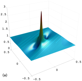
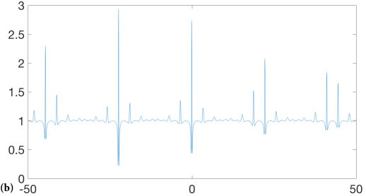
Figure 1: $g=2$:  $\boldsymbol{\alpha}=(-0.0133+i,-0.0033+i,0.0167+i)$; ${\bf k}=(0.5830,0.3147)$; $\langle|\psi_{2}^{{2}}|\rangle=1.0266$; Max amplitude = 3; $K_{2}=8.76680$. (a) Winding of $\mathbb{T}^{2}$;  (b) Plot of $|\psi_{2}(x)|$ corresponding to the winding in (a). According to (10), this configuration of the branchcuts supports rogue waves.

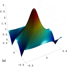
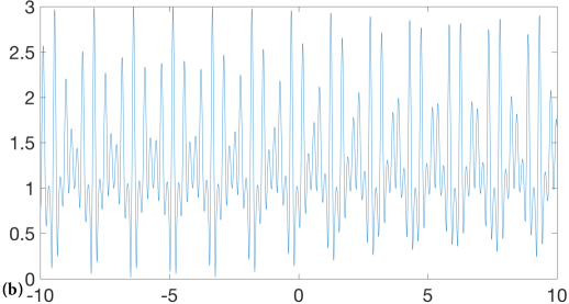
Figure 2: $g=2$:   $\boldsymbol{\alpha}=(-0.6667+i,-0.1667+i,0.8333+i)$; ${\bf k}=(4.58112.6112)$; $\langle|\psi_{2}^{{2}}|\rangle=1.9534$; Max amplitude $|\psi_{2}|_{m}=3$; the rogue wave ratio $K_{2}=4.60735$. (a) Winding of $\mathbb{T}^{2}$;  (b) Plot of $|\psi_{2}(x)|$ corresponding to the winding in (a). According to (10), this configuration of the branchcuts does not support rogue waves.

The black curves in Figs. 1a, 2a show the windings corresponding to the particular choices of the initial point $\boldsymbol{\eta}^{0}$ on the torus. Each winding is parametrised by coordinate $x$, and its direction is defined by the wavenumber vector ${\bf k}$ whose components $k_{j}$ are computed in terms of the branchpoints $\boldsymbol{\alpha}$ by formulae (5). The dependencies $|\psi_{2}(x)|$ corresponding to the particular windings in Figs. 1a, 2a are shown in Figs. 1b and 2b. Given incommensurability of the values of $k_{j}$, each winding covers the corresponding phase torus densely so the probability of the rogue wave occurrence within the given potential $\psi_{2}(x,t;\boldsymbol{\alpha})$ is given by the ratio of the area of the part of the 2D torus confined to the level curve $|\psi_{2}(\eta_{1},\eta_{2})|=C_{r}\langle|\psi_{2}|\rangle$ to the total area of the torus (the unit square).

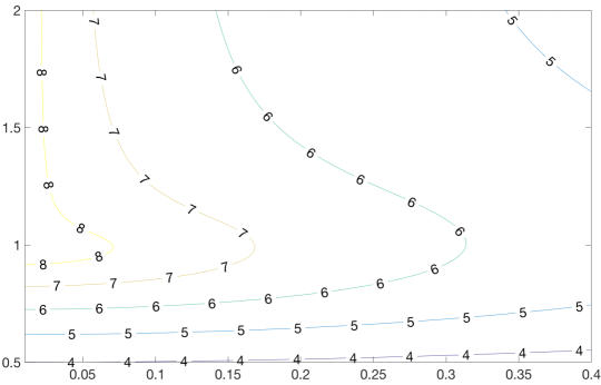
Figure 3: $g=2$. Level curves $K_{2}=4,5,6,7,8$ of the function $K_{2}(\boldsymbol{\alpha},\boldsymbol{\bar{\alpha}})$ (10), where $\alpha_{0}=i$, $\alpha_{1}=-a+ib$, $\alpha_{2}=a+ib$, in the $(a,b)$-plane. Only the potentials with parameters within the area enclosed by the curve $K_{2}=8$ exhibit rogue waves.

It is also instructive to plot the level curves of $K_{2}({\boldsymbol{\alpha},\boldsymbol{\bar{\alpha}}})$ (10) in the space of the spectral parameters $\boldsymbol{\alpha}$. These curves are shown on Fig. 3 for a particular band configuration described below. Without loss of generality we put $\alpha_{0}=i$, i.e. we set one of the bands to be located on the imaginary axis and to have the total height equals to $2$. We shall call it the central band. We then place two other bands of equal height $b_{1}=b_{2}=b$ symmetrically with respect to the central band so that $\alpha_{1}=-a+ib$, $\alpha_{2}=a+ib$. The level curves $b(a)$ of the function $K_{2}(\boldsymbol{\alpha},\boldsymbol{\bar{\alpha}})$ (10) for such potentials are shown in Fig.1 for $K_{2}=4,5,6,7,8$ (only the $a>0$ part of the countour plot is shown, the part with $a<0$ is symmetric with respect to the vertical axis). According to the criterion (10) with $C_{r}=8$, rogue waves are exhibited only by the potentials with spectral parameters in the region enclosed by the curve $K_{2}=8$. One of the immediate conclusions one can make is that, for a genus 2 potential with the described above symmetric band configuration to exhibit rogue waves, it has to have the side bands that: a) have sufficiently large height; and b) are located sufficiently close to the central band. The curve $K_{2}=8$ intersects the imaginary axis ($a=0$) at $b=\frac{\sqrt{8}-1}{2}$. One can see then that the ABs with $a=0$, $\frac{\sqrt{8}-1}{2}<b<1$, the Peregrine breather ($a=0,b=1$) and the KM breathers ($a=0,b>1$) are all inside the “rogue wave region” as expected.

An analogous construction of the finite-band rogue wave identification can be realized for $g>2$, although obviously, the winding of $\mathbb{T}^{g}$ cannot be as easily illustrated. In Figures 4 and 5 we present 3D ($|\psi(x,t)|$) and 2D ($|\psi(x,t^{*})|$) plots of the fNLS finite-band solutions for $g=3$ and $g=4$ respectively. The parameters of both potentials are chosen in such a way that they exhibit rogue waves according to criterion (10).

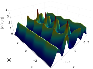
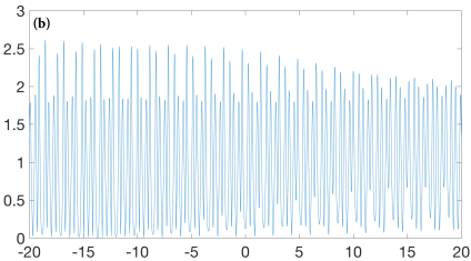
Figure 4: $g=3$; $\boldsymbol{\alpha}=(-0.28808+i,-0.09886+i,0.096952+i,0.28999+i)$; $\left\langle|\psi_{3}|^{2}\right\rangle=1.4563$; $K_{3}=10.9865$. a) Plot of $|\psi_{3}(x,t)|$; b) Plot $|\psi_{3}(x)|$ for a fixed $t$.

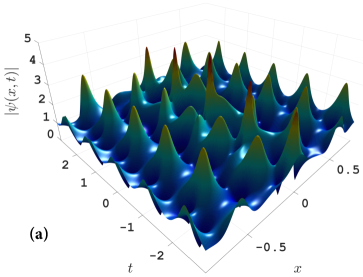
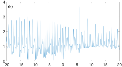
Figure 5: $g=4$; $\boldsymbol{\alpha}=(-0.39271+i,-0.21336+i,0.010556+i,0.20525+i,0.39027+i)$; $\left\langle|\psi_{4}|^{2}\right\rangle=1.6452$; $K_{4}=15.1959$. a) Plot of $|\psi_{4}(x,t)|$; b) Plot $|\psi_{4}(x)|$ for a fixed $t$.

4 Conclusions and outlook

In this paper, we extend the traditional analytical approach to modelling rogue waves by the special SFB solutions of the fNLS equation. Our construction uses finite-band ($g$-phase nonlinear wave, $g\in\mathbb{N}$) solutions of fNLS of whom the known SFB solutions (the Peregrine breather, the Kuznetsov-Ma breather and the Akhmediev breather) are particular, degenerate, cases. In general, a $g$-phase nonlinear wave solution $\psi_{g}$ is defined by a fixed set of $g+1$ vertical (spectral) bands $\gamma_{j}\subset{\mathbb{C}}$ and an arbitrary vector $\boldsymbol{\eta}^{0}$ of $g$ initial phases, where $\boldsymbol{\eta}^{0}\in{\mathbb{T}}^{g}$ - the torus in ${\mathbb{R}}^{g}$. More precisely: i) the spectral bands define a hyperelliptic Riemann surface $\mathcal{R}$ of genus $g$; ii) the finite-band solution $\psi_{g}(x,t)$ is expressed in terms of the Riemann Theta functions (3) on $\mathcal{R}$ so that $|\psi_{g}(x,t)|=f_{g}(\boldsymbol{\eta}(x,t))$, where $\boldsymbol{\eta}(x,t)=\boldsymbol{k}x+\boldsymbol{\omega}t+\boldsymbol{\eta}^{0}$ with $\boldsymbol{\eta}^{0}\in{\mathbb{T}}^{g}$. We introduce the notion of a generalised rogue wave appearing within a $g$-phase nonlinear wave solution $\psi_{g}$ using the traditional amplitude criterion that the maximum of $|\psi_{g}|^{2}$ is at least $C_{r}$ times larger than the mean field $\langle|\psi^{{2}}_{g}|\rangle$. The particular value of $C_{r}$ is at our disposal. To be specific, we use the value $C_{r}=8$ suggested by the previous rogue wave studies. Note that, generically, the wavenumbers $k_{j}$, $j=1,\dots,g$ are incommensurable, so that by ergodicity the mean value $\langle|\psi^{{2}}_{g}|\rangle$ over $\mathbb{T}^{g}$ coincides with mean value of $|\psi^{{2}}_{g}(x,t)|$ over $x\in{\mathbb{R}}$ and $\max_{{\mathbb{T}}^{g}}[f_{g}]=\sup_{x\in{\mathbb{R}}}|\psi_{g}(x,t)|$ with a fixed arbitrary $t$ in both cases.

The recently obtained [7] explicit formula for the maximum of $|\psi_{g}|$ on ${\mathbb{T}}^{g}$ and the formula (A) for $\langle|\psi^{{2}}_{g}|\rangle$ derived in the Appendix allow us to introduce an explicit criterion (10) for the presence of rogue waves within finite-band potentials. Note that this criterion is written in terms of the Riemann surface $\mathcal{R}$: its branchpoints ${\boldsymbol{\alpha},\boldsymbol{\bar{\alpha}}}$, its normalised holomorphic differentials and some abelian integrals. Thus, what is essentially described is not a rogue wave, represented by a particular finite-band solution $\psi_{g}(x,t)$ to the fNLS (1), but a possibility of a rogue wave appearance in the family of the finite-band solutions specified by the spectral branchpoints $\boldsymbol{\alpha},\boldsymbol{\bar{\alpha}}$ and parametrised by $\boldsymbol{\eta}^{0}\in{\mathbb{T}}^{g}$. Our construction thus opens up a consistent way to introduce a statistical description of the generalised rogue waves through the uniform distribution of the initial phase vector $\boldsymbol{\eta}^{0}$ in ${\mathbb{T}}^{g}$. Such a description is currently under the development.

Appendix A Computation of the mean intensity

Here we derive the explicit expression for the average value of $|\psi^{2}(x,t)|$ over $x\in{\mathbb{R}}$. Let $\eta(z)$ be the normalized Abelian integral of the second kind with simple poles at $\infty_{\pm}$ that has expansions

$$\eta(z)=\pm\left(z+R_{0}+R_{1}z^{-1}+O(z^{-2})\right)~{}~{}~{}~{}{\rm so~{}that}~{}~{}~{}~{}~{}\eta^{\prime}(z)=\pm\left(1-R_{1}z^{-2}+O(z^{-3})\right)$$ (A.1)

as $z\rightarrow\infty$, where $R_{0},R_{1}\in{\mathbb{C}}$. It follows from eq. (6.13) of [18] that

$$\langle|\psi^{2}|\rangle=2R_{1}.$$ (A.2)

If $R(z)=\prod_{j=0}^{g}(z-\alpha_{j})^{\frac{1}{2}}(z-\bar{\alpha}_{j})^{\frac{1}{2}}$ then direct calculations yield

$$\frac{1}{R(z)}=z^{-g-1}\left(1+\frac{\sum_{j=0}^{g}a_{j}}{z}+\frac{(\sum_{j=0}^{g}a_{j})^{2}+\sum_{j=0}^{g}(a_{j}^{2}-b_{j}^{2})}{2z^{2}}+O(z^{-3})\right).$$ (A.3)

Representing the normalized meromorphic differential $\eta^{\prime}dz$ near $\infty_{+}$ and taking into account (A.3), we obtain

$$\eta^{\prime}(z)=\frac{z^{g+1}-z^{g}\sum_{j=0}^{g}a_{j}+\sum_{j=1}^{g}\beta_{j}p_{j}(z)}{R(z)},$$ (A.4)

where $\beta_{j}\in{\mathbb{C}}$ and

$$p_{j}(z)=\varkappa_{j,1}z^{g-1}+\varkappa_{j,2}z^{g-2}+\dots+\varkappa_{j,g},\quad j=1,\dots,g$$

are polynomials such that $\nu_{j}=\frac{p_{j}(z)dz}{R(z)}$, $j=1,\dots,g$ are the normalised holomorphic differentials of the hyperelliptic Riemann surface $\mathcal{R}$ of $R(z)$ with the coefficients $\varkappa_{j,i}$ defined by

$$\oint_{\mathbb{A}_{k}}\nu_{j}=\delta_{k,j},$$ (A.5)

where $\delta_{k,j}$ is the Kronecker symbol (see also (6)).

The normalisation condition of $\eta$ means that $\oint_{\mathbb{A}_{k}}\eta^{\prime}(z)dz=0$ for all $k=1,\dots,g$. Thus we obtain

$$\beta_{k}=-\oint_{\mathbb{A}_{k}}\frac{z^{g+1}-z^{g}\sum_{j=0}^{g}a_{j}}{R(z)}dz,~{}~{}~{}~{}~{}~{}~{}k=1,\dots,g.$$ (A.6)

Note that according to (A.1), (A.4), $-R_{1}$ is the $O(z^{-2})$ term in the expansion (A.4) of $\eta^{\prime}$ near $z=\infty$. So, we need to find the leading coefficients $\varkappa_{j,i}$ of the polynomilas $p_{j}(z)=\varkappa_{j,1}z^{g-1}+\varkappa_{j,2}z^{g-2}+\dots+\varkappa_{j,g}$, $j=1,\dots,g$. If

$$\mathbf{A}=\begin{pmatrix}\oint_{\mathbb{A}_{1}}\frac{z^{g-1}dz}{R(z)}&\oint_{\mathbb{A}_{1}}\frac{z^{g-2}dz}{R(z)}&\cdots\oint_{\mathbb{A}_{1}}\frac{dz}{R(z)}\\ \oint_{\mathbb{A}_{2}}\frac{z^{g-1}dz}{R(z)}&\oint_{\mathbb{A}_{2}}\frac{z^{g-2}dz}{R(z)}&\cdots\oint_{\mathbb{A}_{2}}\frac{dz}{R(z)}\\ \cdots&\cdots&\cdots&\\ \oint_{\mathbb{A}_{g}}\frac{z^{g-1}dz}{R(z)}&\oint_{\mathbb{A}_{g}}\frac{z^{g-2}dz}{R(z)}&\cdots\oint_{\mathbb{A}_{g}}\frac{dz}{R(z)}\end{pmatrix}~{}~{}~{}~{}{\rm then}~{}~{}~{}~{}\boldsymbol{\varkappa}_{j}=(\varkappa_{j,1},\dots,\varkappa_{j,g})={\rm Row}_{1}(\mathbf{A}^{-1})$$ (A.7)

So, according to (A.2)-(A.6),

$$\langle|\psi^{2}|\rangle=2\sum_{j=1}^{g}\varkappa_{j,1}\oint_{\mathbb{A}_{j}}\frac{z^{g+1}-z^{g}\sum_{j=0}^{g}a_{j}}{R(z)}dz+\left(\sum_{j=0}^{g}a_{j}\right)^{2}+\sum_{j=0}^{g}(b_{j}^{2}-a_{j}^{2}).$$ (A.8)

In particular, without any loss of generality, we can assume $\sum_{j=0}^{g}a_{j}=0$. Then (A.8) simplifies to (8).

Appendix B SFB limit of $\langle|\psi^{2}|\rangle$

In this subsection we show that the SFB limit (the limit as $a\rightarrow 0$) of $\langle|\psi^{2}|\rangle$ for a two-phase finite-band solution $\psi$ with the spectral bands $\gamma_{0}=[-iq,iq]$, $\gamma_{1}=[\bar{\alpha},\alpha]$ and $\gamma_{2}=[-\alpha,-\bar{\alpha}]$, where $\alpha=a+ib$, coincides with the intensity $q^{2}$ of the background plane wave. Indeed, in this case $R(z)=\sqrt{(z^{2}+q^{2})(z^{2}-\alpha^{2})(z^{2}-\bar{\alpha}^{2})}$ is an odd function when $z\not\in\gamma_{0}$. In this case the leading coefficients $\varkappa_{j,1}$ of the normalized holomorphic differentials

$$\nu_{j}(z)=\frac{p_{j}(z)dz}{R(z)},$$ (B.1)

where $p_{j}(z)=\varkappa_{j,1}z+\varkappa_{j,2}$, can be defined by the system of equations

$$\left(\oint_{\hat{\gamma}_{1}}-\oint_{\hat{\gamma}_{2}}\right)\nu_{1}=1,~{}~{}~{}~{}\left(\oint_{\hat{\gamma}_{1}}-\oint_{\hat{\gamma}_{2}}\right)\nu_{2}=-1.$$ (B.2)

Deforming the contour of integration on $i{\mathbb{R}}$ and using the fact that $R(z)$ is odd, we reduce the system (B.2) to

$$\varkappa_{1,1}=-\varkappa_{2,1}=\frac{1}{2\int_{iq}^{i\infty}\frac{zdz}{R(z)}}.$$ (B.3)

Then, the first sum in (A.8) becomes

$$\sum_{j=1}^{2}\varkappa_{j,1}\oint_{\mathbb{A}_{j}}\frac{z^{3}dz}{R(z)}=\frac{\left(2\int_{iq}^{i\rho}+\int_{\sigma}\right)\frac{z^{3}dz}{R(z)}}{2\int_{iq}^{i\infty}\frac{zdz}{R(z)}},$$ (B.4)

where $\rho>b$ and $\sigma$ is a positively oriented arc of the circle $|z|=\rho$ from $\frac{\pi}{2}$ to $\frac{3\pi}{2}$.

Consider now the case when $b>q$ and $a\rightarrow 0$, that is, the KM breather limit. Taking the limit $a\rightarrow 0$ in (B.4) and using the fact that

$$\lim_{\varepsilon\rightarrow 0^{+}}\int_{-i}^{i}\frac{\phi(z)dz}{\sqrt{z^{2}-\varepsilon^{2}}}=-2\ln\varepsilon\phi(0)+O(1),$$ (B.5)

where $\phi(z)$ is a smooth function that does not depend on $\varepsilon$, we obtain

$$\lim_{a\rightarrow 0^{+}}\sum_{j=1}^{2}\varkappa_{j,1}\oint_{\mathbb{A}_{j}}\frac{z^{3}dz}{R(z)}=-b^{2}.$$ (B.6)

Here we used the fact that the main contribution in the integrals of the right hand side of (B.4) come from a neighborhood of $z=ib$. Thus, we have shown that in the KM limit ( $a\rightarrow 0$) of $\psi$ we have

$$\lim_{a\rightarrow 0^{+}}\langle|\psi^{2}|\rangle=q^{2}.$$ (B.7)

To obtain the limit (B.7) in the case of AB (when $b<q$) breather, we choose $\rho=q$ in (B.4) and represent

$$\int_{\sigma}\frac{z^{3}dz}{R(z)}=\int_{\sigma}\frac{(z^{3}+zb^{2})dz}{R(z)}-2b^{2}\int_{iq}^{i\infty}\frac{zdz}{R(z)}.$$ (B.8)

To complete the proof of (B.7) it remains to notice that $\lim_{a\rightarrow 0}R(z)=\sqrt{z^{2}+q^{2}}(z^{2}+b^{2})$ and, thus,

$$\lim_{a\rightarrow 0^{+}}\int_{\sigma}\frac{(z^{3}+zb^{2})dz}{R(z)}=\int_{\sigma}\frac{zdz}{\sqrt{z^{2}+q^{2}}}.$$ (B.9)

However, the latter integral is zero since the integrand is odd if the contour $\sigma$ is deformed into $[-iq,iq]$. Thus, we proved (B.7) for the AB limit.

References

- [1] D.S. Agafontsev and V.E. Zakharov, Integrable turbulence and formation of rogue waves, Nonlinearity 28, 2791- 2821 (2015).
- [2] N. Akhmediev, A. Ankiewicz and J.M. Soto-Crespo, Rogue waves and rational solutions of the nonlinear Schrödinger equation, Phys. Rev. E 80, 026601 (2009).
- [3] N. Akhmediev, J.M. Soto-Crespo and A. Ankiewicz, Extreme waves that appear from nowhere: On the nature of rogue waves, Phys. Lett. A 373, 2137-2145 (2009).
- [4] N. Akhmediev, J.M. Dudley, D.R. Solli, and S.K. Turitsyn, Recent progress in investigating optical rogue waves, J. Opt. 15, 060201 (2013).
- [5] E.D. Belokolos, A.I. Bobenko, V.Z. Enol’skii, A.R. Its and V.B. Matveev, Algebro-Geometric Approach to Nonlinear Integrable Equations Berlin etc., Springer-Verlag (1994)
- [6] M. Bertola and A. Tovbis, Universality for the focusing nonlinear Schrodinger equation at gradient catastrophe point: rational breathers and poles of the tritronqu e solution to Painlevé I. Comm. Pure Appl. Math. 66, 678-752 (2013).
- [7] M. Bertola and A. Tovbis, Maximum amplitudes of finite-gap solutions for the focusing Nonlinear Schrödinger Equation, arXiv:1601.00875.
- [8] A. Chabchoub, N. Hoffmann, N. Akhmediev, Rogue wave observation in a water wave tank, Phys. Rev. Lett. 106, 204502 (2011) .
- [9] J. M. Dudley, F. Dias, M. Erkintalo, G. Genty, Instabilities, breathers and rogue waves in optics, Nature Photonics 8, 755 - 764 (2014)
- [10] K.B. Dysthe, and K. Trulsen, Note on breather type solutions of the NLS as models for freak-waves. Phys. Scripta 82, 48-52 (1999).
- [11] G.A. El, A.L. Krylov, S.A. Molchanov and S. Venakides, Soliton turbulence as the thermodynamic limit of stochastic soliton lattices, Advances in Nonlinear Mathematics and Science, Physica D 152-153, 653-664 (2001).
- [12] G.A. El, E.G. Khamis and A. Tovbis, Dam break problem for the focusing nonlinear Schrödinger equation and the generation of rogue waves, arXiv:1505.01785
- [13] M. Erkintalo, G. Genty, and J. M. Dudley, Giant dispersive wave generation through soliton collision, Opt. Express 35, 658 - 660 (2010).
- [14] M.G. Forest and J.E. Lee, Geometry and modulation theory for periodic nonlinear Schrödinger equation, in Oscillation Theory, Computation, and Methods of Compensated Compactness, Eds. C. Dafermos et al, IMA Volumes on Mathematics and its Applications 2, (Springer, N.Y., 1987).
- [15] B. Frisquet, B. Kibler, and G. Millot, Collision of Akhmediev Breathers in Nonlinear Fiber Optics, Phys. Rev. X 3, 041032 (2013).
- [16] A.A. Gelash and V.E. Zakharov, Superregular solitonic solutions: A novel scenario for the nonlinear stage of modulation instability, Nonlinearity 27, R1-R39 (2014).
- [17] R.H.J. Grimshaw and A. Tovbis, Rogue waves: analytical predictions, Proc. R. Soc. A 469, 20130094 (2013).
- [18] A.R. Its, V.P. Kotlyarov, Explicit formulas for solutions of the Schrödinger nonlinear equation. Doklady Akad. Nauk Ukrainian SSR, ser.A, 10, 965-968 (1976).
- [19] S. Kamvissis, K. D. T.-R. McLaughlin, and P. D. Miller. Semiclassical soliton ensembles for the focusing nonlinear Schrödinger equation, volume 154 of Annals of Mathematics Studies. Princeton University Press, Princeton, NJ (2003).
- [20] B. Kibler, J. Fatome, C. Finot, G. Millot, F. Dias, G. Genty, N. Akhmediev, and J. M. Dudley, The Peregrine soliton in nonlinear fibre optics, Nature Physics 6, 790-795 (2010)
- [21] B. Kibler, J. Fatome, C. Finot, G. Millot, G. Genty, B. Wetzel, N. Akhmediev, F. Dias, and J. M. Dudley, Observation of Kuznetsov-Ma soliton dynamics in optical fibre, Sci Rep. 2 463 (2012).
- [22] C. Kharif, E. Pelinovsky and A. Slunyaev, Rogue waves in the ocean, vol. 14. Advances in Geophysical and Environmental Mechanics and Mathematics. Berlin, Germany: Springer (2009).
- [23] Y. C. Ma and M. J. Ablowitz, The periodic cubic Schrödinger equation, Stud. Appl. Math. 65, 113-158 (1981)
- [24] S. Nazarenko, Wave turbulence, Lecture Notes in Physics, Springer, 2011
- [25] M. Onorato, A.R. Osborne, M. Serio, C. Brandini, C.T. Stansberg, Observation of strongly non-Gaussian statistics for random sea surface gravity waves in wave flume experiments, Physical Review E 70 (2004) 067302.
- [26] M. Onorato, S. Residori, U. Bortolozzo, A. Montina, and F.T. Arecchi, Rogue waves and their generating mechanisms in different physical contexts, Phys. Rep. 528 47 - 89 (2013).
- [27] A. R. Osborne, Nonlinear ocean waves and the inverse scattering transform. Amsterdam, The Netherlands: Elsevier (2010)
- [28] S. Randoux, P. Suret and G. El, Identification of rogue waves from scattering transform analysis of periodized waveforms, arXiv:1512.04707, submitted.
- [29] V.I. Shrira and V.V. Geogjaev, What makes the Peregrine soliton so special as a prototype of freak waves?, J. Eng. Math. 67, 11-22 (2010).
- [30] D.R. Solli, C. Ropers, P. Koonath, and B. Jalali, Optical rogue waves, Nature 450, 1054-1057 (2007).
- [31] J. Soto-Crespo, N. Devine, and N. Akhmediev, Integrable turbulence and rogue waves: breathers or solitons? Phys. Rev. Lett. 116, 103901 (2016).
- [32] E.R. Tracy and H.H. Chen, Nonlinear self-modulation: An exactly solvable model Phys. Rev. A 37, 815-839 (1988).
- [33] A. Tovbis, S. Venakides, and X. Zhou. On semiclassical (zero dispersion limit) solutions of the focusing nonlinear Schrödinger equation. Comm. Pure Appl. Math., 57(7), 877-985, (2004).
- [34] P. Walczak, S. Randoux, P. Suret, Optical Rogue Waves in integrable turbulence, Phys. Rev.Lett 114, 143903 (2015).
- [35] O. Wright, Effective integration of ultra-elliptic solutions of the focusing nonlinear Schrödinger equation, Physica D 321-322, 16 - 38 (2016)
- [36] V.E. Zakharov and A.B. Shabat, Exact theory of two-dimensional self-focusing and one-dimensional self-modulation of waves in nonlinear media, Sov. Phys. JETP 34, 62-69 (1972).
- [37] V.E. Zakharov, Turbulence in integrable systems, Stud. Appl. Math. 122, 219 - 234 (2009).
- [38] V.E. Zakharov and A.A. Gelash, Nonlinear stage of modulational instability, Phys. Rev. Lett. 111, 054101 (2013).