Magnetohydrodynamic simulations of mechanical stellar feedback in a sheet-like molecular cloud

Abstract

We have used the AMR hydrodynamic code, MG, to perform 3D magnetohydrodynamic simulations with self-gravity of stellar feedback in a sheet-like molecular cloud formed through the action of the thermal instability. We simulate the interaction of the mechanical energy input from a 15 M_⊙ star and a 40 M_⊙ star into a 100 pc-diameter 17000 M_⊙ cloud with a corrugated sheet morphology that in projection appears filamentary. The stellar winds are introduced using appropriate Geneva stellar evolution models. In the 15 M_⊙ star case, the wind forms a narrow bipolar cavity with minimal effect on the parent cloud. In the 40 M_⊙ star case, the more powerful stellar wind creates a large cylindrical cavity through the centre of the cloud. After 12.5 Myrs and 4.97 Myrs respectively, the massive stars explode as supernovae (SNe). In the 15 M_⊙ star case, the SN material and energy is primarily deposited into the molecular cloud surroundings over $\sim 10^{5}$ years before the SN remnant escapes the cloud. In the 40 M_⊙ star case, a significant fraction of the SN material and energy rapidly escapes the molecular cloud along the wind cavity in a few tens of kiloyears. Both SN events compress the molecular cloud material around them to higher densities (so may trigger further star formation), and strengthen the magnetic field, typically by factors of 2-3 but up to a factor of 10. Our simulations are relevant to observations of bubbles in flattened ring-like molecular clouds and bipolar HII regions.

1 Introduction

Stellar feedback, through both winds and supernovae (SNe), is recognized as having significant influence on galactic and extra-galactic scales. Winds and SNe not only chemically enrich the interstellar medium (ISM), but also drive structural evolution and motion within it. Massive stars embedded within molecular clouds most likely affect star formation, with the ability to both inhibit further star formation, as their winds and ionizing radiation disperse the molecular gas, and in some cases trigger new star formation (Koenig et al., 2012) and even new cluster formation (Beuther, Linz & Henning, 2008; Gray & Scannapieco, 2011). Winds are particularly important to consider as they can introduce similar amounts of mass and energy as SNe and strongly affect the environment into which SNe explode.

Stellar wind feedback into an inhomogeneous environment has been studied by Harper-Clark & Murray (2009). They postulate that the non-uniform surrounding medium causes gaps in the swept-up shell surrounding the wind-blown bubble where some of the high-pressure gas in the bubble interior can leak out. Lopez et al. (2011) supported this scenario concluding that such leakage may be occurring within 30 Doradus. They also conclude that direct stellar radiation pressure dominates the interior dynamics, but this claim has proved far more controversial, and other works are in favour of the thermal pressure of hot X-ray emitting plasma shaping the large-scale structure and dynamics in 30 Doradus (e.g. Pellegrini et al., 2011). More recently, Lopez et al. (2014) concluded that the warm ionised gas pressure dominates in HII regions on scales of $10-100$ pc.

The possibility that the pressure exerted by stellar radiation may be dynamically important in massive young stellar clusters has also received much attention in recent years, with Krumholz & Matzner (2009), Fall, Krumholz & Matzner (2010) and Murray, Quataert & Thompson (2010) all arguing that radiation pressure is the dominant feedback mechanism. However, these works disagree on the net momentum coupling between the radiation field and the gas, partially because this depends on the degree of inhomogeneity of the gas and the effect that this has on the radiation field (e.g. Krumholz & Thompson, 2012). Complementary work on the ionised gas pressure has shown that ionization feedback into a highly inhomogeneous medium is not very effective at high cluster masses (Dale & Bonnell, 2011), but becomes more so at lower masses (Dale, Ercolano & Bonnell, 2012; Walch et al., 2012).

Recent work has also explored the effect of supernovae on the multi-phase ISM and molecular clouds (Gatto et al., 2015; Walch & Naab, 2015; Walch et al., 2015; Girichidis et al., 2015; Körtgen, 2015; Körtgen et al., 2016). Girichidis et al. (2015) employed 3D MHD simulations of the ISM in a vertically stratified box including self-gravity, an external potential due to the stellar component of the galactic disc, and stellar feedback in the form of an interstellar radiation field and SNe. They also used a sophisticated cooling prescription based on full tracking of a chemical network following the abundances of H⁺, H, H₂, C⁺ and CO, taking into account shielding in a consistent fashion. They varied the SN feedback with different rates, clustering and positioning in the disc. Positioning, either randomly or at peak density locations, had a major impact on the dynamics. Only for random SN positions is the energy injected in sufficiently low-density environments as to reduce energy losses and enhance the kinetic coupling of the SNe with the gas, leading to more realistic velocity dispersions and strong outflows. SNe placed in density peaks do not drive any noticeable outflow. However, the effect of the SN-preceding stellar wind was not accounted for and very recent simulations (Simpson et al., 2016) accounting for the production of cosmic rays in supernova events has shown that they are able to drive outflows from SNe placed at density peaks, with similar mass loading as obtained from random placement of SNe with no cosmic rays.

Offner & Arce (2015) used MHD simulations to model winds launching within turbulent molecular clouds and explored the impact of wind properties on cloud morphology and turbulence. They used the AMR code ORION to model an isothermal molecular cloud. In 7 out of 9 cases they use a $\beta$ of 0.1 - a magnetic pressure $10\times$ greater than the thermal pressure and hence a magnetic field that strongly influences the evolution. They introduce stellar winds with constant mass-loss rates and constant velocities. They found that the winds do not produce clear features in turbulent statistics such as the Fourier spectra of density and momentum, but do impact on the Fourier velocity spectrum. They showed that stellar mass-loss rates for individual stars must be greater than 10^-7 M_⊙ yr^-1, similar to those estimated from observations, in order to reproduce shell properties.

Körtgen, in his recent PhD work (Körtgen, 2015) and resulting publication (Körtgen et al., 2016), performed MHD simulations of converging turbulent (Mach $\sim$ 2) warm neutral medium flows in order to form magnetised and turbulent molecular clouds. SN feedback was then introduced into these clouds, through the form of thermal and kinetic energy according to E_SN=10⁵¹ erg with E_th=0.65 E_SN and E_kin=0.35 E_SN in a spherical control volume of radius 0.06 pc. They found that SN feedback alone failed to disrupt the entire molecular cloud, but was able to disperse small-sized ($\sim$10 pc) regions on timescales of less than 1 Myr. Efficient radiative cooling of the SN remnant as well as strong compression of the surrounding gas result in non-persistent energy and momentum input from the SNe. Multiple clustered SNe with short intervals (at a rate much higher than typical IMF calculations) are able to combine to form large hot bubbles that disperse larger regions of the parental cloud, and give an upper limit on the efficiency of SN feedback given the assumptions in the model. Kim & Ostriker (2015) also analysed SNe exploding in a two-phase ISM (see also Martizzi, Faucher-Giguère & Quataert, 2015) with no feedback prior to the SNe and found the net momentum input is nearly independent of the environment. However, this conclusion may well change if pre-SN (wind and ionizing radiation) feedback is considered.

Simulations of momentum-driven or isothermal winds (Dale et al., 2014; Dale, Ercolano & Bonnell, 2015; Offner & Arce, 2015) give a lower limit to their impact. Pre-SN feedback has been found to enhance the impact of SNe (Rogers & Pittard, 2013; Fierlinger et al., 2016), and, in whole galaxy models, clears dense gas from star forming regions, reducing the star formation rate (e.g., Agertz et al., 2013). However, whole galaxy models remain very sensitive to assumptions in the feedback scheme.

In recent work by our group (Rogers & Pittard, 2013, 2014), we examined the extent to which the mechanical energy input from a cluster of massive stars is confined by and shapes the local environment, focusing on feedback due to SNe and the preceding stellar winds. 3D hydrodynamic models simulated the interaction of the mechanical energy from three massive stars with a giant molecular cloud clump containing 3240 M_⊙ of material within a 4 pc radius. The stars were evolved through 3 idealized evolutionary phases: O-star main sequence (MS), red supergiant (RSG), and Wolf-Rayet (WR), before exploding as SNe. The clump structure was based upon the simulations of Vázquez-Semadini et al. (2008) of turbulent and clumpy molecular clouds. The combined cluster wind from the three O-stars was found to blow out of the inhomogeneous molecular clump along paths of least resistance. Hot, high-speed gas flows away from the cluster through these low-density channels, into which denser clump material is entrained. These channels are directly related to the initial cloud structure. Molecular material is gradually removed by the cluster wind during which mass-loading factors in excess of several 100 were obtained, but this process is relatively slow and a substantial amount of molecular material remains near the cluster when the first SN occurs. However, because this material has a small volume filling fraction, the environment is highly porous to the transport of wind and SN energy, and the majority of the wind energy and essentially all of the SN energy escaped to the wider surroundings. Nevertheless, the winds appeared to be better at removing molecular material from the cluster environment, despite injecting less energy then the SNe. The molecular material was found to be almost completely dispersed and destroyed after 6 Myr. This work demonstrated the complexity of the interaction of a cluster wind with an inhomogeneous environment, and is far removed from simple spherically symmetric models.

A key conclusion of Rogers & Pittard (2013) is that massive stars that form at high density locations are able to disperse surrounding material through the action of their winds, aiding the relatively unhindered escape of SN energy. Therefore, the effect of the preceding stellar wind phase should be considered when calculating the impact of SN explosions on the surrounding gaseous environment.

In our previous work the simulated results were strongly linked to the initial clump structure and did not include magnetic fields, realistic stellar wind evolution or self-gravity. A parameterised heating/cooling rate per unit volume was also employed. In the work presented here we make several improvements in our exploration of the effect of stellar feedback on molecular clouds. Firstly, we use a self-consistent cloud structure, which has formed naturally under the influence of the thermal instability, magnetic fields and self-gravity (Wareing et al., 2016, hereafter Paper I). In our previous paper feedback occurred into a roughly spherical, but inhomogeneous, region. Here we explore the other extreme, where the stellar feedback occurs into a sheet-like structure, as formed when the initial plasma beta is unity. Such flattened cloud morphologies have been inferred in recent work by Beaumont & Williams (2010). We also examine feedback from a single star (of mass 15 M_⊙ and 40 M_⊙), employing realistic Geneva stellar evolution tracks for the time-varying wind properties, rather than the multiple stars and simplified wind evolution considered by Rogers & Pittard (2013). Finally, we use a more accurate heating and cooling prescription (albeit leaving photoionisation and the full tracking of chemical species and their interplay to a future work).

In the next section, we present our numerical method and define the initial conditions used in our model. In Section 3 we present and discuss our results. In Section 4 we consider the global energy, density, phase and mixing behaviour. In Section 5 we further analyse those results with comparison to previous work and relevant recent observational results. We summarise and conclude the work in Section 6.

2 Numerical Methods and initial conditions

2.1 Numerical methods

We present 3D, magneto-hydrodynamical (MHD) simulations of stellar feedback with self-gravity using the established astrophysical code MG (Falle, 1991) as recently used in Paper I. The code employs an upwind, conservative shock-capturing scheme and is able to employ multiple processors through parallelisation with the message passing interface (MPI) library. MG uses piece-wise linear cell interpolation to solve the Eulerian equations of hydrodynamics. The Riemann problem is solved at cell interfaces to obtain the conserved fluxes for the time update. Integration in time proceeds according to a second-order accurate Godunov method (Godunov, 1959). A Kurganov Tadmor Riemann solver is used in this work (Kurganov & Tadmor, 2000). Self-gravity is computed using a full-approximation multigrid to solve the Poisson equation. The magnetic field components are cell-centered and the $\nabla\cdot B$ criterion is enforced using divergence cleaning (Dedner et al., 2002).

The adaptive mesh refinement (AMR) method (Falle, 2005) employs an unstructured grid approach. By default, the two coarsest levels (G0 and G1) cover the whole computational domain; finer grids need not do so. Refinement or derefinement is based on error. Where there are steep gradients of variable magnitudes such as at filaments, flow boundaries or discontinuities, this automated meshing strategy allows the mesh to be more refined than in more uniform areas. Each level is generated from its predecessor by doubling the number of computational grid cells in each spatial direction. This technique enables the generation of fine grids in regions of high spatial and temporal variation, and conversely, relatively coarse grids where the flow field is numerically smooth. Defragmentation of the AMR grid in hardware memory is performed at every time-step, gaining further speed improvements for negligible cost through reallocation of cells into consecutive memory locations. The simulations presented below employed 8 levels of AMR at a minimum, with resolution tests to 10 levels of AMR. Physical domain sizes and hence physical resolutions are as detailed below.

2.2 Heating and cooling processes

Care has been taken to continue our implementation of realistic heating and cooling as used in Paper I, as it is the balance of these processes that formed the initial molecular cloud condition. In the ISM, heating as defined by the coefficient $\Gamma$, varies with increasing density as the starlight, soft X-ray and cosmic ray flux are attenuated by the high column density associated with dense clouds. Because the exact form of the attenuation depends on details which remain uncertain (e.g. the size and abundance of PAHs), the heating rate at T $\leq$ 10⁴ K is similarly uncertain. In this work, following on from the filament formation work, we have assumed that $\Gamma=2\times 10^{-26}$ erg s^-1 (independent of density or temperature). For the low-temperature cooling ($\leq 10^{4}$ K), we have followed the detailed prescription of Koyama & Inutsuka (2000), fitted by Koyama & Inutsuka (2002), and corrected according to Vázquez-Semadini et al. (2007), namely

$$\begin{array}[]{ll}\displaystyle{\frac{{\Lambda(T)}}{\Gamma}=}&\displaystyle{{10^{7}}\exp\left({\frac{{-1.184\times{{10}^{5}}}}{{T+1000}}}\right)}\\ &\\ &\displaystyle{+1.4\times{10^{-2}}\sqrt{T}\exp\left({\frac{{-92}}{T}}\right)}.\end{array}$$ (1)

At higher temperatures we have followed the prescription of Gnat & Ferland (2012) who used CLOUDY 10.00, enabling us to define cooling rates over the temperature range from 10 K to 10⁸ K. This has been implemented into MG as a lookup table for efficient computation.

2.3 Initial conditions

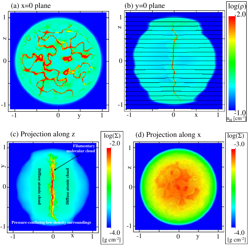
Figure 1: Initial condition. Snapshot of a $\beta=1.0$ filamentary cloud after 38.8 Myrs of evolution used as the initial condition in this work. Shown are logarithm of mass density on planes (a) x=0 and (b) y=0 and projected column density perpendicular to the field direction in (c) and parallel to the field direction in (d). Length is scaled in units of 50 pc. Field lines are shown where appropriate.

Paper I focused on the study of filamentary molecular cloud formation under the influence of the thermal instability (Parker, 1953; Field, 1965). In that work, we examined the evolution of diffuse clouds varying $\beta$, the ratio of thermal pressure to magnetic pressure. We examined three cases, $\beta$ = 0.1, 1.0 and $\infty$ (equivalent to the hydrodynamic case of zero magnetic field). Following Paper I, the initial condition consists of a stationary cloud of radius 50 pc with a number density of hydrogen throughout the cloud of n_H = 1.1 cm^-3. In the cloud, 10% density variations about the uniform initial density were introduced, giving the cloud a total mass of $\sim$17,000 M_⊙. The pressure was set according to the local density and thermal equilibrium between heating and cooling prescriptions at P_eq/k = $4700\pm 300$ K cm^-3, resulting in an initial temperature T_eq = $4300\pm 700$ K (an unstable part of the equilibrium curve - for more details see Paper I). The pressure of the lower density (n_H = 0.1 cm^-3) surroundings was set equal to that of the unperturbed cloud.

The domain was initially threaded with uniform $B$-field along the $x$ direction, i.e. B = $B_{0}$ $\hat{\textbf{I}}_{x}$. For the moderate field case of $\beta=1.0$, the initial cloud condition was pressure equality, i.e. the thermal pressure of the initial cloud with n_H = 1.1 cm^-3 led to $B_{0}$ = 1.15 $\mu$G. This is a typical Galactic field strength at an inner ($\sim$ 4 kpc) location. Evolved molecular clouds have been noted to have magnetic field strengths over 10$\times$ greater than these, but it is not clear how these field strengths have been generated. Having shown in Paper I that filament formation under the action of the thermal instability cannot intensify the magnetic field, we also examine in this work whether stellar feedback generating super-sonic, super-Alfvénic motions can intensify the field to such levels.

The computational domain consists of a 150 pc³ box with free-flow boundary conditions (non-periodic for self-gravity) and AMR level G0 containing 4³ cells. Eight levels of AMR mean an effective resolution of 512³ cells, although G5 with 128³ cells is the finest fully populated level (rather than the MG default of G1, in order to resolve the action of the thermal instability). Such a large number of AMR levels is employed in order to efficiently compute the self-gravity on the coarsest levels and also fully resolve the structures formed in the molecular cloud. The finest physical resolution is 0.293 pc. The large number of AMR levels is computationally costly. Each 3D MHD simulation with stellar feedback and self-gravity presented here with 8 AMR levels took approximately 60,000 CPUhours ($\sim$10-12 48-hour cycles on 128 cores of the MARC1 high performance computing facility at Leeds), so 120,000 CPUhours for the two runs presented. Supporting investigations including a parameter exploration of the initial condition (see Paper I), high resolution tests, stellar feedback tests & tests with other stellar masses etc. mean the total computational cost of the work presented in this paper approaches 200,000 CPUhours. A large-scale parameter exploration is thus prohibitively expensive. Regarding the choice of number of AMR levels used for the base case, each further level of AMR introduces a computational-cost-multiplier of between 3 and 4 for this model, thus making complete higher resolution simulations prohibitively expensive at this time.

The influence of the thermal instability causes the cloud to evolve into multiple clumps without any magnetic field and into a filamentary structure under the influence of magnetic field. Specifically, with $\beta=\infty$, molecular clumps formed across the diffuse cloud. In the other two cases, molecular filaments formed across the cloud, eventually forming intersecting bundles of filaments and corrugated sheets. Seen in projection, the filaments closely resemble those observed. Densities, column densities, widths, velocity dispersions and separations all resemble derived properties of observed filaments. Self-gravity accelerates the contraction of the cloud and makes the cloud more filamentary. Besides exploring the importance of the thermal instability in molecular cloud evolution, the secondary aim of Paper I was to provide a more realistic initial condition for this work, by including more accurate heating and cooling, the effect of thermal instability, self-gravity and magnetic fields, as compared to our previous feedback studies (Rogers & Pittard, 2013, 2014).

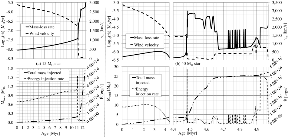
Figure 2: Stellar evolution tracks (Vink et al., 2000, 2001; Ekström et al., 2012) for the (a) 15 M_⊙ star and the (b) 40 M_⊙ star, showing mass-loss rate and wind velocity on the upper graphs, and energy injection rate and total injected mass on the lower graphs.

In this work, we take as our initial condition a repeat of a $\beta=1.0$ filamentary cloud simulation following the method of Paper I. Different random seeds results in a simulation that is qualitatively the same as the $\beta=1.0$ case in Paper I, but quantitatively different. After 32.9 Myrs of evolution, densities in the filamentary structures formed in this new simulation have reached 100 cm^-3 - the density threshold often used for injection of stars in similar simulation work (e.g., Fogerty et al., 2016). At a density of 100 cm^-3, the free-fall time due to gravity is 5.89 Myrs. Therefore, we choose to introduce stars into our simulation after 38.8 Myrs of evolution. We show snapshots of this initial condition in Figure 1 and refer the interested reader to Paper I for a full description of the evolutionary process that led to the formation of this cloud. It is important to note though that this time-scale should not be considered as the ‘age’ of the parent molecular cloud - this is the length of time required to go from a diffuse cloud with an average density of n_H = 1.1 cm^-3 to a structured molecular cloud where feedback can be introduced. Grid levels G6 and G7 are 18% and 10% populated respectively at this simulation time, leading to an initial total of $18.5\times 10^{6}$ grid cells.

We consider two scenarios, each employing this initial condition, in order to examine the effect of stellar feedback.

2.3.1 Scenario 1 - a 15 M_⊙ star

In this scenario we introduce a 15 M_⊙ star at the position (x,y,z) = (-0.025, 0.0, 0.0125) where the coordinates are given in scaled code units. This location has been selected as the highest density location in the sheet, closest to the centre of the domain. Further, enough mass is present in a spherical volume with a 5-cell radius centred at this point, that can form a 15 M_⊙ star assuming $\sim$100% material conversion from cloud to star. For this first investigation, the mass is removed at the switch on of the stellar wind, t_wind=0. Whilst this may seem inconsistent, if the mass is left in the injection region, the stellar wind rapidly and unrealistically cools and hence the feedback effects are significantly underestimated. The location of the star remains constant throughout this work. In future work, we plan to convert the mass into a ‘star’ particle following the method in MG of Van Loo, Butler & Tan (2013) and Van Loo et al. (2015). The star can then move through the domain whilst feeding back into the domain through winds and SNe and remain consistent with self-gravity in the simulation. The stable position of the molecular cloud does not require particles for these simulations.

For the stellar evolution, a 15 M_⊙ non-rotating Geneva stellar evolution model calculated by Ekström et al. (2012) is used in order to provide a realistic mass-loss rate over the lifetime of the star. We use the mass, temperature, luminosity and metallicity together with the prescriptions of Vink et al. (2000, 2001) in order to calculate the wind velocity. Ekström et al. (2012) describe lower mass star tracks, but the minimum stellar mass that can be used with the Vink et al. (2000, 2001) method is 15 M_⊙. The calculated mass-loss rate and wind velocity are shown in Fig. 2(a). Also shown in Fig. 2(a) are the energy injection rate and total injected mass. The stellar wind is introduced as a mass and energy source, directly using the mass-loss rate as a density source and the kinetic energy of the wind as a thermalised energy source. No momentum source is introduced in this work. The wind is introduced over the same spherical region of the grid with a radius of 5 cells at the finest grid level that was used to remove the equivalent or greater mass of molecular material. An advected scalar, $\alpha_{wind}$, previously set to zero throughout the grid, is set to 1 in the wind injection region in order to track the movement and mixing of the wind material. The total mass and total energy injected by the star prior to supernova explosion are 1.75 M_⊙ and $1.05\times 10^{49}$ erg respectively. The wind rapidly expands outside the injection region.

After 12.5 Myrs, the star explodes as a SN, injecting 10 M_⊙ of stellar material and 10⁵¹ ergs of energy into the same wind injection volume. The mass and energy is injected over 500 yrs, roughly consistent with the time taken for a remnant to reach the size of the injection volume. A second advected scalar, $\alpha_{SN}$, previously set to zero throughout the grid, is set to 1 in the supernova injection region in order to track the movement and mixing of the SN material. At this time the wind scalar $\alpha_{wind}$ is set to zero.

Limited numerical convergence testing has shown the introduction of a finer grid level accelerates the wind more quickly given the increased source terms, but that the simulations here capture the large-scale interaction of the wind and filamentary molecular cloud that we are interested in. Computationally, even the use of a single further fine AMR level becomes very expensive and time-consuming, as discussed in the preceding subsection.

Gravity plays less of a role during the stellar wind phase and the early SN phase, due to the comparatively powerful dynamics even in the 15 M_⊙ star case, but we continue to include it for consistency within the cloud and to explore the evolution post-SN when it again plays more of a role. However, assessing gravity’s relative importance post-SN, as compared to the flow dynamics induced by the SNR, the triggered thermal instability, and any numerical effects now present is difficult.

2.3.2 Scenario 2 - a 40 M_⊙ star

In this scenario we introduce a 40 M_⊙ star using the same method and position as in scenario 1. A spherical volume of material slightly larger than in the previous scenario was removed in order to conserve mass in introducing the star, but again this was small enough to be unimportant in terms of the global evolution of the wind-cloud interaction. A 40 M_⊙ non-rotating stellar evolution model calculated by Ekström et al. (2012) is used in order to provide a realistic mass-loss rate over the lifetime of the star in the same manner as in the first scenario. The calculated mass-loss rate and wind velocity are shown in Fig. 2(b). Also shown in Fig. 2(b) are the energy injection rate and total injected mass. The total mass and total energy injected by the star prior to supernova explosion are 27.2 M_⊙ and $2.50\times 10^{50}$ erg respectively, comparable to the material and energy introduced in a SN event. After 4.97 Myrs, the star explodes as a SN in the same manner as in the first scenario.

2.4 Neglected processes and simplifications

This work represents a step forward in modelling mechanical stellar feedback in molecular cloud conditions. We have necessarily made a number of simplifications and approximations, a number of which have been outlined above but for completeness we consider the rest here.

We neglect the role of carbon monoxide (CO). Without a full treatment of heating according to column density and shielding to allow the formation of CO, it is difficult to justify the inclusion of any CO effects into the cooling curve, although this was done in our previous work through an amendment to the parameterised low temperature cooling (Rogers & Pittard, 2013, 2014). In terms of molecular cloud evolution, we found in tests carried out as part of our previous work (Wareing et al., 2016) that the increased cooling introduced by CO at lower temperature allows the clumps and filaments to cool further (and increase in density) to temperatures on the order of 10-15 K. With regard to this work, the tenuous stellar winds and SNe interact with this material and it is therefore likely that we observe the maximum effect that winds and SNe can have on the filamentary structures, as higher densities in these structures will lead to longer ablation times.

We have not included sink particles at this time, but, as already noted, the cloud does not contract further due to self-gravity and we plan to adopt this technique in future work. However, there is, as yet, no really satisfactory way of identifying the gravitationally collapsing regions that can be turned into sink particles.

Photoionisation and radiative feedback are not included at this time. Inclusion of such should speed up the destruction of molecular material. Having said this, photoevaporation may be suppressed in regions where the ram or thermal pressure of the surrounding medium is greater than the pressure of the evaporating flow (Dyson, 1994). Either way, the results of Simpson et al. (2016) suggest further study in this area is required as a matter of urgency and we are developing numerical techniques in order to include these effects.

We also note that dust can dramatically affect the cooling within hot bubbles if it can be continuously replenished, perhaps by the evaporation/destruction of dense clumps (Everett & Churchwell, 2010) which will also mass-load the bubble (see e.g. Pittard et al., 2001a, b). The presence of dust will also affect the photoionization rate throughout the cloud. Clearly the effects of dust warrant further study.

3 Results

In this section we present our results. We present both 2D slices through the computational domains created within MG and 3D contour and volume visualisations, created using the VisIt software (VisIt Collaboration, 2012). Line profiles on the 2D slices are shown in the Appendix. Raw data can be obtained from http://doi.org/10.5518/114.

3.1 Scenario 1 - a 15 M_⊙ star

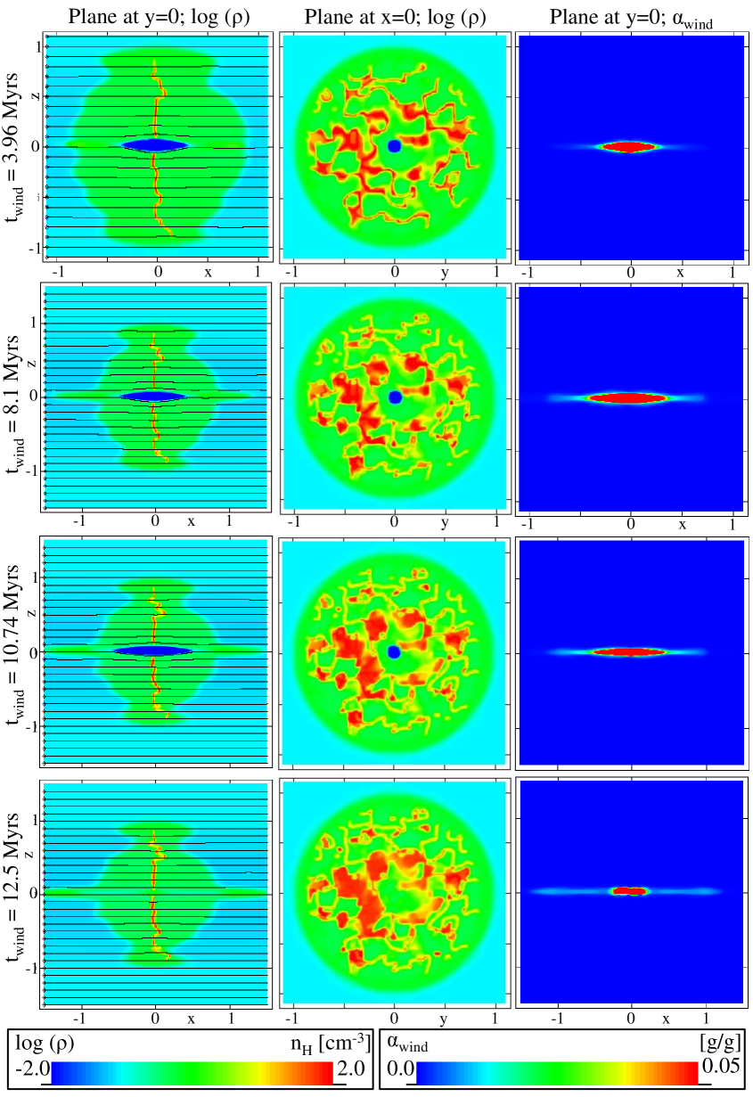
Figure 3: Cloud-wind interaction during the lifetime of a 15 M_⊙ star. Shown is: column 1 - the logarithm of mass density on the plane at $y=0$; column 2 - the logarithm of mass density on the plane at $x=0$; column 3 - the wind scalar on the plane at $y=0$. Length is scaled in units of 50 pc. For line profiles on these planes, see Figure 16.

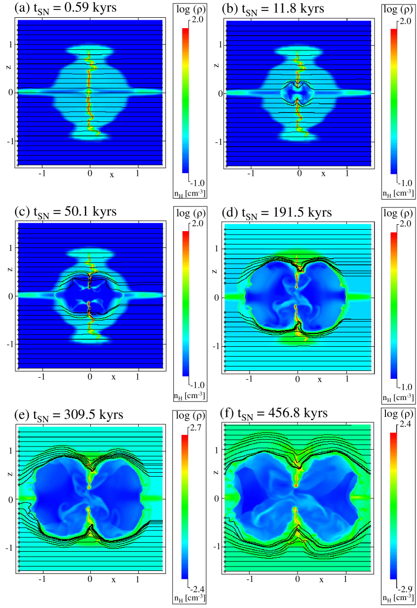
Figure 4: SN-wind-cloud interaction during the SN phase of a 15 M_⊙ star. Shown is the logarithm of mass density on the plane at y=0 at various times through the SN evolution. Length is scaled in units of 50 pc. For line profiles on these planes, see Figure 17.

In Fig. 3 (see also Fig. 16) we show density slices through the domain during the evolution of the 15 M_⊙ star up to the end of its life. The low mass-loss rate and corresponding low energy injection rate have minimal effect on the cloud structure, generating only a small bipolar cavity parallel to the magnetic field at the location of the star. This creates a hole in the corrugated sheet of filamentary molecular cloud, but does not emerge from the surrounding diffuse cloud, only pushing material ahead of it along fieldlines, as can be seen in the left column of Fig. 3. A plane at $z=0$ rather than at $y=0$ reveals the same structure for all timepoints. This structure is a result of the weak wind in combination with the comparatively high-density filamentary cloud structure, collimating the weak stellar wind into a bipolar outflow away from the plane of the cloud at $y=0$. The filamentary molecular cloud structure is relatively unaffected across the corrugated sheet of the cloud, with only a 5 pc diameter hole punched through the 100 pc-diameter sheet at the location of the star, as can be seen in the middle column of Fig. 3. Examining the movement of the stellar wind material as shown in the right column of Fig. 3, we see that very little wind material gets more than 25 pc away from the star.

During the red super giant (RSG) phase of evolution, from t_wind=11.2 Myr until its SN explosion, the slow dense wind deposits considerable amounts of material into the cavity formed by the earlier wind, as can be seen in the change of density around the star between rows 3 and 4 of Fig. 3. The RSG wind has a lower energy injection rate and so the main sequence wind-blown-bubble collapses somewhat. There is no Wolf-Rayet (WR) stage during the stellar evolution of the 15 M_⊙ star (cf. Georgy et al., 2015).

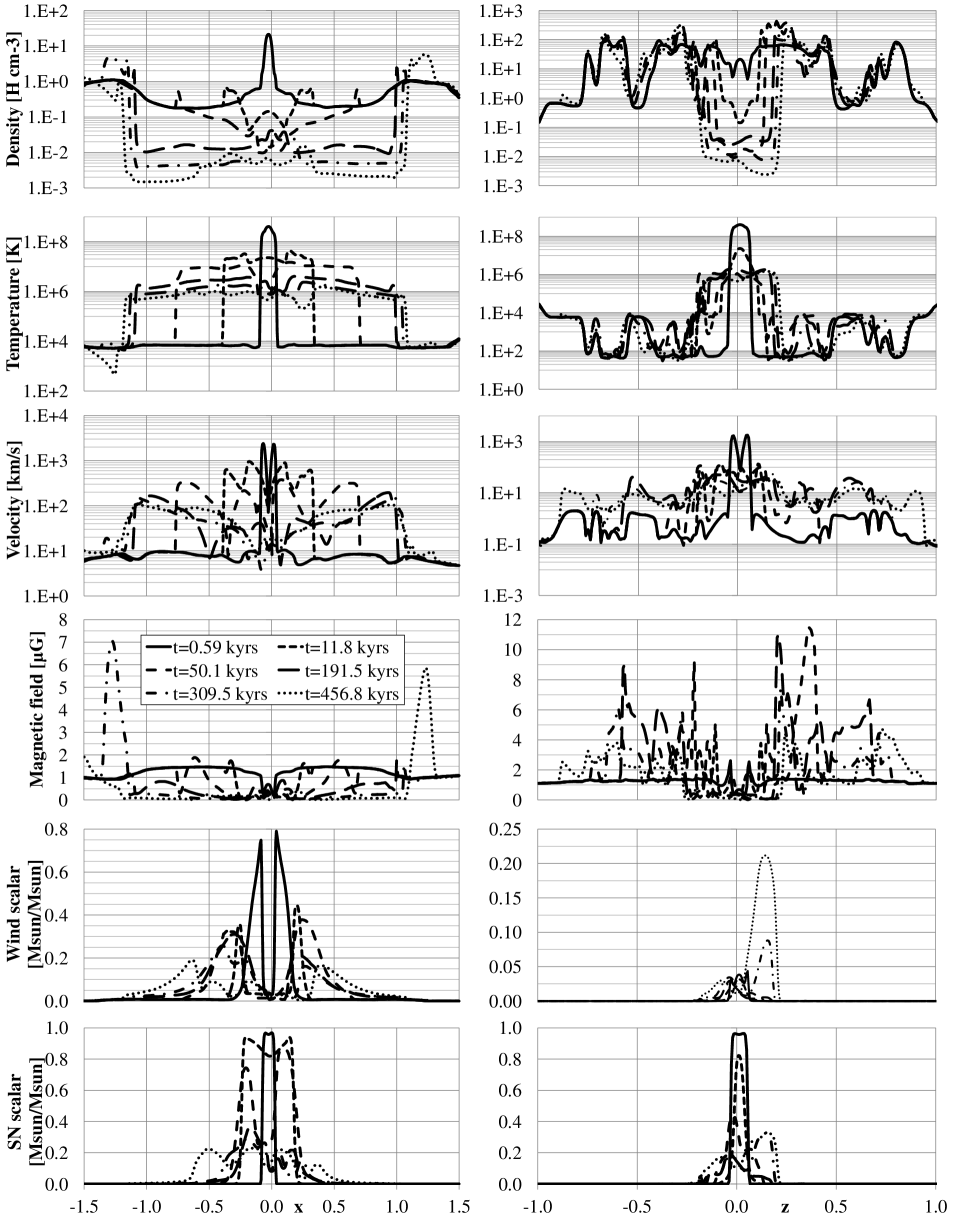
Figure 17: Line profiles of the SN-wind-cloud structure shown in Figure 4 for the 15 M_⊙ star simulation. Left column: profiles along the magnetic field in the $x$ direction at the location of the central star ($y$,$z$) = (0.0, 0.0125). Right column: profiles across the magnetic field in the $z$ direction and across the corrugated sheet of the molecular cloud at the location of the central star ($x$,$y$) = (-0.025, 0.0).

The accumulation of RSG wind material around the location of the star affects the early evolution of the following SN, as shown in Figs. 4 and 17. However, since the total mass-lost during the RSG stage ($\sim 1.5$ M_⊙) is much less than the mass of the SN ejecta, the RSG wind can only be a small perturbation to the initial development of the SN remnant. By 11.8 kyrs, as shown in Fig. 4(b), the forward shock of the SN is clear. The expansion is only being hindered by the comparatively high-density corrugated sheet of filamentary molecular cloud. Elsewhere, the forward shock is expanding most quickly into the remains of the wind cavity, sweeping up tenuous wind material. Given the nature of the explosive SN event, the pressure-driven forward shock is also expanding into the lower density surroundings of remnant diffuse cloud, sweeping up material from the cloud ahead of the shock. The high-density filamentary structure is beginning to be ablated by the SN remnant, mixing molecular, wind and SN material in flows away from the stellar location. In Fig. 4(c) the more rapid expansion through the wind cavity is clearer, as the thin shells sweeping up the tenuous wind material are furtherest from the stellar location by this time, 50 kyrs after the SN event. The sweeping up of the magnetic field lines as the shell expands is also clear. Panels (d), (e) and (f) of Fig. 4 show the continued expansion of the SN remnant with ablation of the molecular cloud until it reaches the edge of the computational domain. The progression of shocks internal to the SN remnant are particularly clear comparing panels (e) and (f), carrying material away from the ablating molecular cloud and introducing internal density structure to the SN remnant.

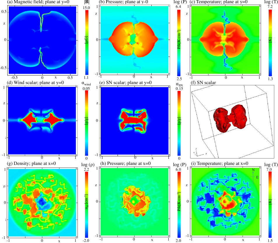
Figure 5: Details of the SN-wind-cloud interaction 50.1 kyrs into the SN phase of a 15 M_⊙ star. Length is scaled in units of 50 pc.

In Fig. 5 we show more detail of the SN remnant at one point in time, 50.1 kyrs after the SN explosion, as previously shown in the third row of Fig. 4. In Fig. 5(a) we show the magnetic field strength, detailing the enhancements in the shell and at the edges of the filamentary structure alluded to in the previous paragraph. Magnetic field strengths in the swept up shell have increased from the initial uniform 1.15 $\mu$G by up to a factor of 4 around the shell away from the filamentary cloud. At the edges of the corrugated sheet of the filamentary molecular cloud structure, magnetic field strengths have increased by a factor of 10 or more, up to 16 $\mu$G at most. This strengthening is not confined to the ablating edge of the molecular cloud closest to the star location, but extends and strengthens along the filament towards the location of the SN forward shock. The correlation with adiabatic compression of material would suggest this amplification is due to adiabatic compression. Generation of shear flows by the passage of the SN shock may also have contributed and led to the highest fields observed in specific locations. There is no evidence in this simulation of small-scale dynamo effects.

It is thus apparent that SN events in molecular clouds can increase magnetic field strengths, through shock-driven compression of the molecular cloud itself, in line with observed increased magnetic field strength in molecular clouds. Examining the evolution of the field before and after this time, it is apparent that the magnetic field strengthens in the filamentary molecular cloud from 2-3 $\mu$G a short time after the SN, to the temporary peak of 16 $\mu$G, reducing to at most 11 $\mu$G 191.5 kyrs after the SN (Fig. 4(d)) and then 7.4 $\mu$G 309.5 kyrs after the SN (Fig. 4(e)). Localised regions of increased field strength then persist in the filamentary molecular cloud, decreasing from 7-8 $\mu$G at this time until long after the SN event and wider destruction of the cloud occurs, discussed later. Temporary localised increases in magnetic field strength around the edge of the expanding SN remnant are briefly apparent, reaching up to 8 $\mu$G. It is possible to conclude that SN events in molecular clouds can temporarily increase magnetic field strengths by a factor of 10 over timescales of 50 kyrs after the SN and create persisting magnetic fields four times stronger than the ambient field strength for hundreds of thousands of years after the SN.

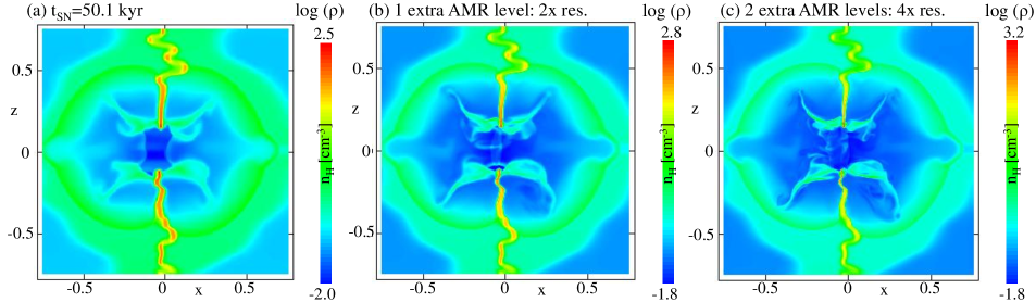
Figure 6: Results of a resolution test simulating the SN phase of a 15 M_⊙ star. (a) 8 levels of AMR, as presented previously; (b) one extra level of AMR doubling the resolution; (c) two extra levels of AMR, doubling the resolution again from (b). Length is scaled in units of 50 pc.

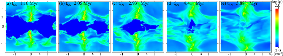
Figure 7: Late SN-wind-cloud interaction during the SN phase of a 15 M_⊙ star. Shown is the logarithm of mass density on the plane at y=0 at various times through the SNR evolution. The SN forward shock has evolved off the grid and hence boundary effects are now present. Ideally a larger grid is required, but the figure is shown to demonstrate the possible late-stage evolution of the SN-affected filamentary cloud. Length is scaled in units of 50 pc.

In the rest of Fig. 5 we show the further details of the expanding SN in order to highlight various properties of the remnant at this time. Figs. 5(b) and 5(c) show the pressure and temperature in the SN remnant, clearly illustrating the pressure-driven nature of the SN at this time and the high temperatures (up to 10⁷ K) behind the forward shock. The low temperatures in the filamentary molecular cloud are also clear in Fig 5(c), persisting through the passage of the SN shock. The distribution of stellar wind material at this time is shown in Fig 5(d) - note the scaling from 0 to 0.05 to elucidate the extended distribution of wind material. The forward shock of the SN has passed over nearly all the wind material, raising its temperature to 10⁷ K, but densities are low, hence any emission from this material will be minimal. The distribution of material ejected from the star in the SN event is shown in Fig. 5(e), again scaled to elucidate it’s furthest extent. The distribution at this time has been shaped by the escape of ejected material from the star’s location along the wind cavity. The motion of SN ejecta directly along the $z=0$ axis has been impeded by the wind material, with which it now mixes. Ablation of the molecular material from the inside edges of the hole in the molecular cloud has led to the ‘X’ shape (missing the central section) apparent in density, pressure and temperature plots on the $y=0$ plane and made conspicuous by the absence of wind and SN material in the scalar plots. It should be noted that in the arms of the ‘X’ is hot ($>$10⁵ K), comparatively high density ($>$10 cm^-3) material that originated in the molecular cloud and that is likely to be emitting relatively strongly in a SN remnant such as this.

The volume rendition in Fig. 5(f) shows the full extent of the ejected SN material - reminiscent of a mushroom cloud reflected about the plane of the molecular cloud ($x\sim 0$), with ‘dimples’ at the top of the cloud showing the impeding effect of the swept-up stellar wind material. Shown in panels (g), (h) and (i) of Fig. 5 are the density, pressure and temperature on the $x=0$ plane, to show the extent to which the expanding SN remnant has affected the corrugated sheet of the molecular cloud. Compared to plots of density on the same plane in Fig. 3, there is little to no difference outside the SNR, where the SN has compressed and heated some of the molecular material. Placing a compass on the figure (as shown in Fig. 5(i)), in the regions to the south-east the SN has expanded the furthest and raised the pressure and temperature of material swept up by the forward shock. This is not surprising, as consideration of the same region in Fig. 3 shows the lowest density structure in this direction and hence naively the least resistance to an expanding SN shock.

In order to reassure ourselves that we are resolving the cooling lengths in this simulation, we have checked that this is the case and whilst the resolution is close to the cooling length in the expanding SN shock, the cell size is always less than the cooling length. To reassure ourselves further, we have also performed extra, high resolution simulations of the very early SN phase, starting from the point at which the SN ejecta and energy have just been injected. We show the results of this resolution test in Fig. 6. In panel (a) we show the distribution of density on a logarithmic scale as previously shown in Fig. 3, 50.1 kyrs after the SN explosion. We plot the density on the same plane at the same time for a simulation with 1 extra level of AMR (doubling the resolution) in panel (b) and a further extra level of AMR, equalling 10 in all, in panel (c), doubling the resolution again. Whilst the qualitative details of the internal shock structures vary within the SN remnant, it’s clear that the expanding forward shock is in the same place, as is the ablating edge of the molecular cloud, and trails of ablated material away from this edge. The internal structure may be more sharply resolved in both higher resolution cases, but this is not particularly important to the overall evolution of the cloud and the cost of such simulations prohibits execution at these higher resolutions. Each further level of AMR introduces a computational-cost-multiplier of between 3 and 4 to the base resolution cost of 60,000 CPUhours per feedback case. It is notable though that the extra resolution allows for the refined capture of the compression of the corrugated molecular sheet behind the ablating edges, reaching densities up to 1500 cm^-3 in the highest resolution simulation. Such densities might be high enough to trigger star formation at these locations.

In Fig. 7 we show the late time evolution of this simulation. Note that the following results are indicative of the resulting evolution, and should not be taken too literally, since the forward shock has now left the computational domain and boundary effects have come into play. Nevertheless, they can be used as a guide to the sort of behaviour one might expect to see. We are particularly interested in the fate of the corrugated molecular sheet. At 1.164 Myr after the SN (panel (a)), the filamentary molecular cloud is still reasonably recognizable in the simulation, albeit being driven away from the location of the SN, overcoming the self-gravity of the cloud. However, after 3 Myrs (panel (c)), the molecular cloud is clearly dispersing, with little high density structure (on this plane) compared to earlier times, and by 6 Myrs, the cloud has been dispersed. Self-gravity in the dispersed clumps is now likely to dominate their evolution, possibly leading to further star formation. It is highly likely that the disruption of the molecular cloud is caused by the SN event, but to be sure future simulations with a larger computational volume are necessary. Further questions over the fate of the remaining molecular material and whether the SN triggers any further formation of cold material by disrupting the thermal stability of the cloud material are addressed in Section 4.

3.2 Scenario 2 - a 40 M_⊙ star

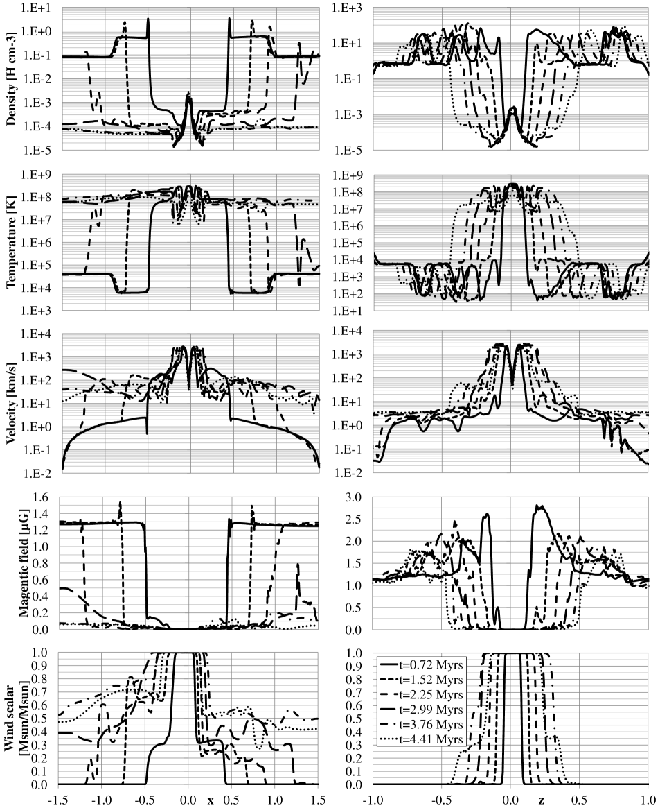
Figure 18: Line profiles of the wind-cloud structure shown in Figure 8 for the 40 M_⊙ star simulation. Left column: profiles along the magnetic field in the $x$ direction at the location of the central star ($y$,$z$) = (0.0, 0.0125). Right column: profiles across the magnetic field in the $z$ direction and across the corrugated sheet of the molecular cloud at the location of the central star ($x$,$y$) = (-0.025, 0.0).

In Fig. 8 (see also Fig. 18) we show the logarithm of density on a plane at $y=0$ including the location of the 40 M_⊙ star. At only 0.722 Myrs into the main sequence evolution of the star, the impact on the molecular cloud is significant and clearly different from the 15 M_⊙ star case, as shown in Fig. 8(a). The stellar wind is forming a bipolar cavity around the location of the star, with a narrow-waist coincident with the corrugated sheet structure of the molecular cloud. This time, the wind is powerful enough to sweep up diffuse cloud material ahead of it and affect the magnetic field, trebling the magnetic field strength in the swept up diffuse cloud material. Again, indications are that this is due to adiabatic compression. No magnetic field is injected with the stellar wind in these simulations but in general the stellar magnetic field is not expected to be strong enough to significantly affect the dynamics.

The bipolar cavity grows as the wind establishes a distinct reverse shock by 1.52 Myrs, shown in Fig. 8(b). By 2.25 Myrs, the bipolar wind bubble has expanded to the edge of the diffuse cloud and is 100 pc across. Magnetic field strengths have dropped to 2.5 $\mu$G from the earlier peak. Once the stellar wind has broken out of the diffuse cloud, it rapidly accelerates away into the surrounding tenuous medium. This results in a cylindrical cavity through the cloud by 3.76 Myrs, whose diameter has only increased slightly by 4.41 Myrs when the star evolves off the main sequence. By 4.41 Myrs, the corrugated sheet structure of the molecular cloud has been driven back to the edge of the cylindrical cavity, approximately 25 pc from the location of the star. As such, the star now exists inside a large cylindrical tunnel-like cavity punching through the centre of the molecular cloud. This cavity is filled with hot, tenuous stellar wind material, moving away from the star at speeds over 1000 km s^-1. Much of the injected wind material flows out of the cavity at the edge of the grid, taking $\sim 10^{5}$ years to do so. The orientation of this channel is stable throughout the latter stages of stellar evolution.

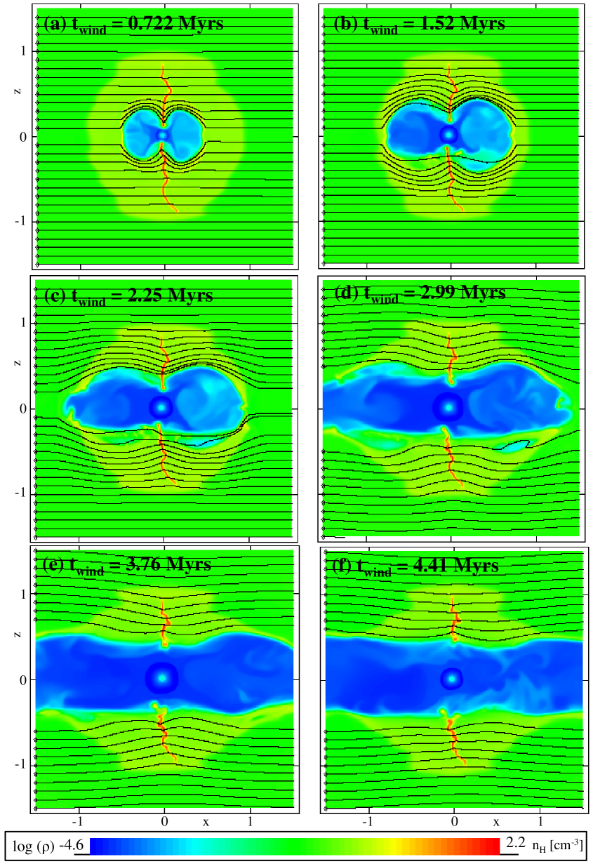
Figure 8: Intra-molecular cloud evolution of the wind-blown-bubble from a 40 M_⊙ star. Shown is the logarithm of mass density on a plane at y=0. Length is scaled in units of 50 pc. For line profiles on these planes, see Figure 18.

Next, the star enters the LBV phase. The wind mass-loss rate increases by two orders of magnitude to $\sim 10^{-4}$ M_⊙ yr^-1, and the terminal wind speed reduces to $\sim 100$ km s^-1. This slow dense wind sweeps up a new shell into the previous wind phase and forms a high density environment around the location of the star, which eventually contains $\sim 20$ M_⊙ of LBV wind material. This phase lasts approximately 200 kyrs and is followed by the WR phase of stellar evolution, where a variable, faster, less dense wind sweeps up the LBV wind over the course of the final 400 kyrs of the star’s life. The resulting environment into which the SN mass and energy are injected is shown in Fig. 9(a). A 25 pc diameter near-spherical high density structure is located in the centre of the stellar wind cavity, isolated from the molecular cloud by the 25 pc radial extent of the main sequence wind tunnel-like cavity.

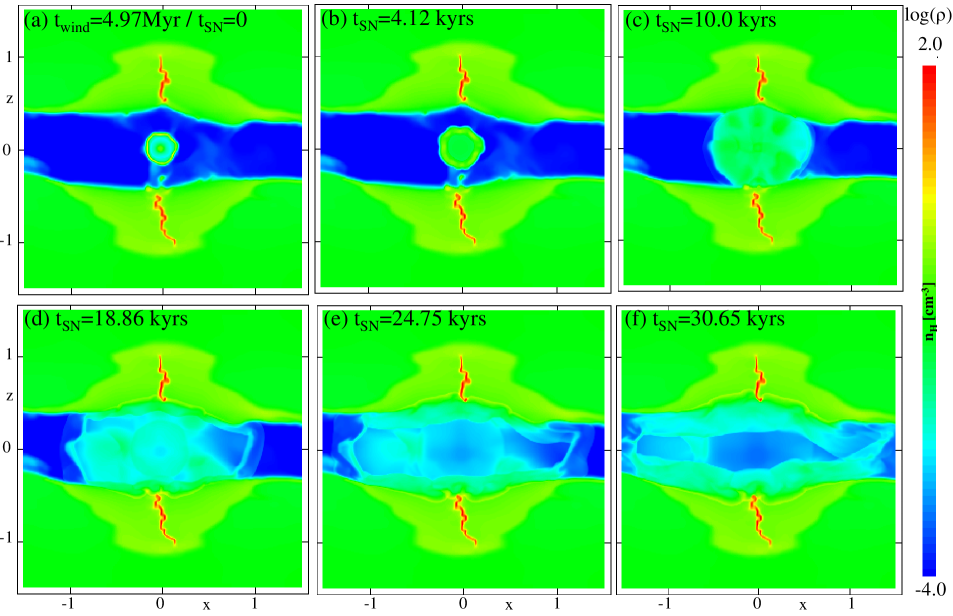
Figure 9: Intra-wind cavity evolution of the SN phase of a 40 M_⊙ star. Shown is the logarithm of mass density on a plane at y=0. Length is scaled in units of 50 pc. For line profiles on these planes, see Figure 19.

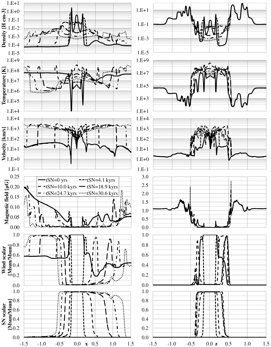
Figure 19: Line profiles of the early-time SN-wind-cloud structure shown in Figure 9 for the 40 M_⊙ star simulation. Left column: profiles along the magnetic field in the $x$ direction at the location of the central star ($y$,$z$) = (0.0, 0.0125). Right column: profiles across the magnetic field in the $z$ direction and across the corrugated sheet of the molecular cloud at the location of the central star ($x$,$y$) = (-0.025, 0.0).

In the rest of Fig. 9 (see also Fig. 19), we show the evolution of the SNR. After 4 kyrs the SNR shock has propagated through the LBV/WR wind-blown-bubble material and is beginning to interact with the tenuous wind material from the MS phase of evolution. The expanding remnant remains almost spherical until it reaches the high density “wall” of the tunnel-like MS wind cavity, encountering then the high density filamentary molecular cloud and the diffuse cloud surrounding the location of the former star. In contrast, the SNR expands almost unhindered along the MS wind cavity towards the edge of the domain. After only 19 kyrs, the SN shell has reached 50 pc along the cavity from the location of the SN (travelling at an average speed of 2600 km s^-1. Elsewhere, the progress of the SN forward shock has been dramatically slowed by the denser diffuse cloud and molecular sheet. Reverse shocks are also reflecting back from the cavity wall towards the central axis of the cavity, progressing rapidly throughout the cavity as shown in panels (d), (e) and (f) of Fig. 9. After 30.65 kyrs, the SN shell has reached the edge of the computational domain, 75 pc from the SN location, along the wind cavity. As a comparison, the SN in the case of the 15 M_⊙ star took 50 kyrs to reach the edge of the diffuse cloud and a further 400 kyrs to expand to the edge of the same computational domain. The introduction of the strong stellar wind from the 40 M_⊙ star has wide-reaching consequences; the majority of the SN energy and material is able to leave the molecular cloud relatively unhindered, due to the cavity formed by the stellar wind.

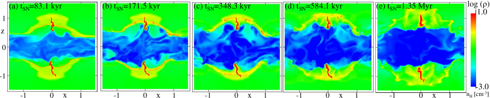
Figure 10: SN-cloud interaction during the post-SN-cavity-interaction phase of a SN from a 40 M_⊙ star. Shown is the logarithm of mass density on a plane at y=0. Length is scaled in units of 50 pc. For line profiles on these planes, see Figure 20.

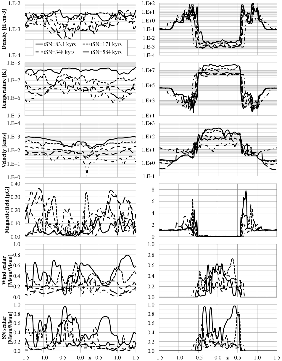
Figure 20: Line profiles of the SN-wind-cloud structure shown in Figure 10 for the 40 M_⊙ star simulation. Left column: profiles along the magnetic field in the $x$ direction at the location of the central star ($y$,$z$) = (0.0, 0.0125). Right column: profiles across the magnetic field in the $z$ direction and across the corrugated sheet of the molecular cloud at the location of the central star ($x$,$y$) = (-0.025, 0.0).

During this short intra-cavity stage, the SN remnant also begins to expand into the filamentary molecular cloud and its parent diffuse cloud. It takes considerably longer to pass through these regions - 1.35 Myrs. We show snapshots of this period in Fig. 10 (see also Fig. 20). 83 kyrs after the SN explosion, as shown in Fig. 10(a), the SN shock is sweeping up diffuse cloud material ahead of it, leaving material behind the shock to flow into the cavity. The flow along the cavity and off the grid is primarily driven by the earlier expansion of the remnant out of the cavity, but also by reverse shocks off the cavity walls. This effect is further pronounced in Figs. 10(b) and 10(c), 171.5 and 348.3 kyrs after the SN explosion. The slowing down of the forward shock as it sweeps up the diffuse cloud between these times is also apparent. By 584 kyrs after the explosion (Fig. 10(d)), the SN remnant has expanded and cooled far enough to reach the radiative phase of evolution. The shell becomes subject to Rayleigh-Taylor instabilities and breaks up into individual clumps, as can be seen most clearly in Fig. 10(e), 1.35 Myrs after the initial SN event. Interestingly, the filamentary molecular cloud survives this phase of its evolution remarkably intact, apart from the large hole in the centre of the corrugated sheet that was originally caused by the stellar wind. This hole has expanded in diameter by 20% during its interaction with the SN. The corrugated sheet has also expanded outwards, driven by the SN, but has retained its form and high density. Magnetic fields in and around the filament and at the edges of the SN remnant are temporarily increased by factors of 3 or 4, but no more, and by 1.35 Myrs have returned to around 2 $\mu$G, having started out in the diffuse cloud at 1.15 $\mu$G.

The accuracy of this phase of the simulation can be questioned, due to the SN shock having expanded along the cavity off the grid. Progress of the SN shock into the diffuse cloud and filamentary sheet does not appear to be affected by boundary effects that may have affected the evolution of the intra-cavity material, and for this reason we can be reasonably confident in the description of the evolution until 1.35 Myrs post explosion. After 1.35 Myrs, the SN evolution follows a path remarkably similar to the 15 M_⊙ star case, refilling the domain and eventually disrupting the host molecular cloud on the same 6 Myr timescale. It is likely that in this case, physical causes include the interactions of the shocks that bounced off the inside of the cavity and back towards the location of the star. These then progress across the whole cavity and generate further shock echoes, which all drive weaker yet destructive shocks into the molecular cloud. Gravity also begins to play a role at this time, but because boundary effects will progressively affect the simulation past this point we do not show any further details, which will require additional larger domain simulations.

4 Analysis

4.1 Energy

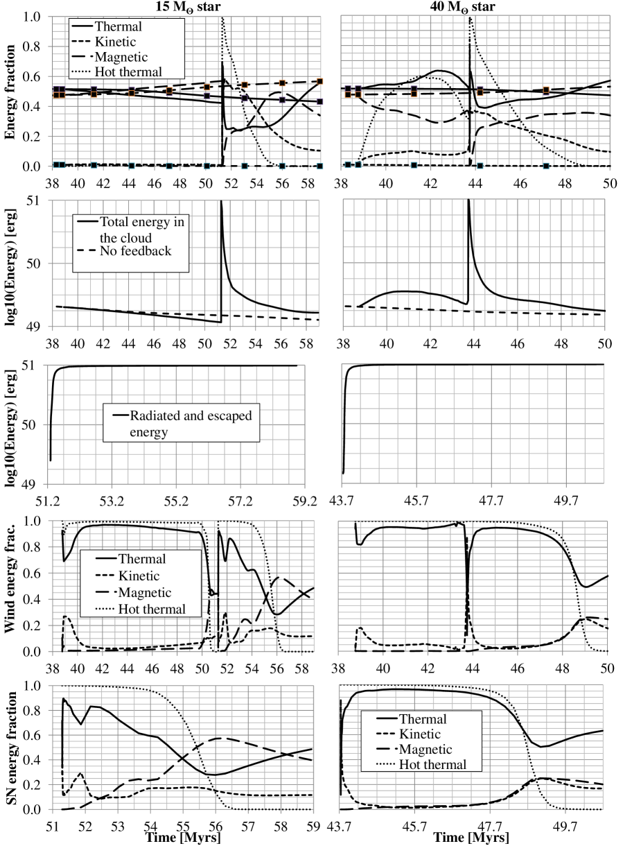
Figure 11: Time profiles of energy fractions, totals and escaped amounts of energy in the cloud and separately for wind energy and SN energy. The thermal, kinetic and magnetic energy fractions together sum to 1.0 i.e. we are ignoring the change in gravitational energy. The ‘hot thermal’ profile indicates the fraction of the thermal energy which is hot (above $10^{4}$ K), and so also has a range between 0.0 and 1.0. In the first row, lines with markers indicate the energy behaviour in the cloud with no stellar feedback. In the third row, the “radiated and escaped energy” is the total cloud energy subtracted from the injected energy of the SN, 10⁵¹ erg.

Across the first row of Fig. 11 we show how the distribution of energy between kinetic, magnetic, thermal and hot thermal (i.e. material above 10,000K) varies over time following the introduction of stellar feedback, with reference to a simulation of the cloud evolution without feedback (indicated by lines with markers). The thermal, kinetic and magnetic energy fractions together sum to 1.0 i.e. we are ignoring gravitational energy.

In the 15 M_⊙ star case, the fractions do not change considerably during the wind phase, as compared to the reference case. This was expected from the minimal dynamic and structural impact the star has on the cloud. It is also supported by the fact that the majority of the energy in the wind is thermal, as shown in the fourth row of Fig. 11, highlighting the minimal kinetic energy introduced by the relatively weak stellar wind. In fact the star introduces so little energy, that the overall energy in the cloud reduces during the wind phase, as compared to the ‘no feedback’ reference case. This likely arises due to a combination of: i) some small fraction of material leaving the cloud; ii) relatively efficient radiation of the energy injected by the stellar wind, perhaps due to weakly compressing and heating neighbouring cloud material.

The introduction of the thermalised SN kinetic energy is most obvious in the total energy plot, as the discontinuity at 51.3 Myrs. Since the SN energy is injected thermally, both the thermal energy and the ‘hot thermal’ phase spike at this time. Over time, the thermal fraction drops off to 25%, as some of the SN thermal energy transforms into kinetic energy, and as the SNR cools. For the first $10^{5}$ yrs, the SNR is expanding into diffuse cloud with $n_{\rm H}\sim 1\,{\rm cm\,s^{-1}}$ and into the cold corrugated sheet with $n_{\rm H}\sim 100\,{\rm cm\,s^{-1}}$. The timescale for the transition of a SNR into its radiative phase was determined by Blondin et al. (1998) to be $\approx 1.5t_{\rm tr}$, where $t_{\rm tr}$ is given by their Eq. 3. For these densities, we expect the remnant to become radiative after $\approx 5\times 10^{4}$ yr expanding into the diffuse cloud and $\approx 4\times 10^{3}$ yr expanding into the cold corruagted sheet. This is in keeping with our simulation results: in the “radiated and escaped energy” plot, 80% of the SN energy radiates away prior to the SNR starting to leave the grid ($\approx 0.3$ Myrs after the explosion, or 51.6 Myrs since the start of the simulation).

Once the SN remnant has left the grid, it is no surprise that the kinetic energy fraction falls against the rising thermal and magnetic energy fractions (although with no injection of magnetic energy, in reality the total magnetic energy is either maintained or decreases over time as material leaves the grid). The variations of energy fraction during the SN phase are most clearly shown in the plot of the SN energy fraction on the fifth row. We remind the reader that all plots should be interpreted with caution at times after the SNR first reaches the boundaries of the numerical domain.

For the 40 M_⊙ star case, the stellar wind has a considerably larger effect on the energy fractions. The star introduces a large amount of hot thermal and kinetic energy, raising both fractions considerably above the reference case. The magnetic energy fraction goes down, but this reflects an increase of total energy in the simulation during the wind phase (as shown in the second row) rather than a reduction of magnetic energy. Given that the wind blows a hot bubble, it’s likely that radiative losses are responsible for the drop in total energy approaching the end of the star’s life, before the introduction of 10⁵¹ erg in the SN event. In this case, the SN would appear to have less of an effect on the energy fractions than the 15 M_⊙ star - no surprise given the ease with which SN ejecta leave the cloud along the tunnel. Closer inspection has shown that there is a spike in kinetic energy up to 0.8 for 30,000 years post-SN as the SN material is ejected down the tunnel and out of the cloud. This fraction drops rapidly as the SN shell expands into the cloud, as shown in the second row and in detail in the final row of the figure, where the initial kinetic energy peak is clearer. 5 Myrs post-SN, the energy balances change considerably from their previous post-SN behaviour. It is most likely that this is influenced by boundary effects after the forward shock of the SNR has crossed the grid boundary. As such, we again reiterate that results late after the SN must be treated with caution.

4.2 Maximum density

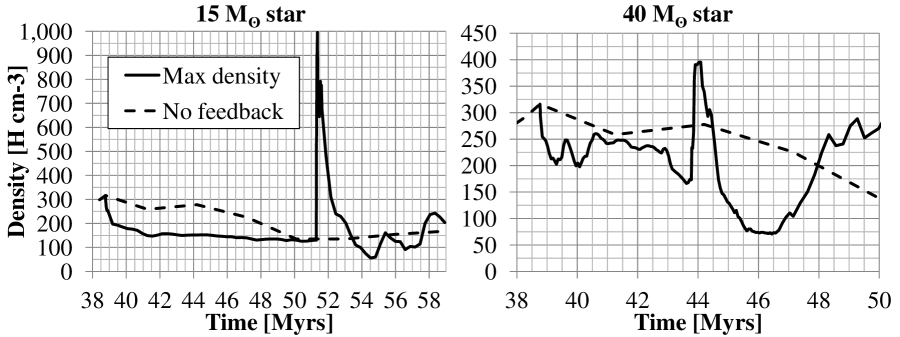
Figure 12: Maximum density in the two stellar feedback simulations (solid lines) shown with the maximum density in a continued simulation of the same initial conditions without feedback (dotted line) for reference.

In Fig. 12 we show the maximum densities reached in the simulations, compared to the maximum density at the same time in the reference case without stellar feedback. In the 15 M_⊙ star case, the maximum density during the wind phase is considerably lower than the reference case, until just before the SN. Since we chose to position the star and inject the wind at the highest density location close to the centre of the cloud, this behaviour reflects that choice. The final wind stages inject a considerable amount of mass at low velocity around the star’s location, raising the density back to ‘no feedback’ levels. The SN instantly raises the density in the injection location, but the spikes seen in the plot are not associated with the SN injection, but instead with compression of the filamentary cloud by the SN shock, leading to maximum densities far above the ‘no feedback’ case for nearly 2 Myrs after the SN event. Later peaks in the maximum density plot for the 15 M_⊙ star may be associated with the formation of new cold material after SN affected material returns to the thermally unstable phase. These peaks again cross the threshold at which we formed our star and at which other authors inject stars, which if incorporated would ‘trigger’ further star formation.

The plot of maximum density for the 40 M_⊙ star shows a much more variable maximum density during the wind phase. Initially this is less than the reference case, but at times it comes close to returning to the reference case. The variations are not due to the variations in the stellar wind - it is relatively steady for 4 Myrs as shown in Fig. 2 - but instead are due to the compressional effect the stellar wind has on the cloud, creating first the bipolar bubble (generating the spikes in maximum density) and then blowing out the tunnel through the cloud (reducing the maximum density once the tunnel has become established). The final stellar wind stages and the SN event are the cause of the peak in maximum density at 44 Myrs. There is not enough energy to drive as high a peak as in the 15 M_⊙ star case; a lot of the energy is ‘vented’ along the tunnel and therefore there is less compression of the gas. The rise in density is sustained for a period after the SN event of approximately 0.5 Myrs, before maximum densities in this case drop far below the reference case. Whilst a significant fraction of the SN ejecta may have left the cloud along the tunnel, clearly the SNR still has a strong effect on the parent cloud over the next 3 Myrs, reducing densities far below the reference case and based on our criterion, turning off any further star formation. After this time, maximum densities in the simulation begin to rise again. This correlates with the increase in cold material triggered by both the wind and the SN forcing material back into the thermally unstable phase, discussed in more detail in the next section.

4.3 Phases

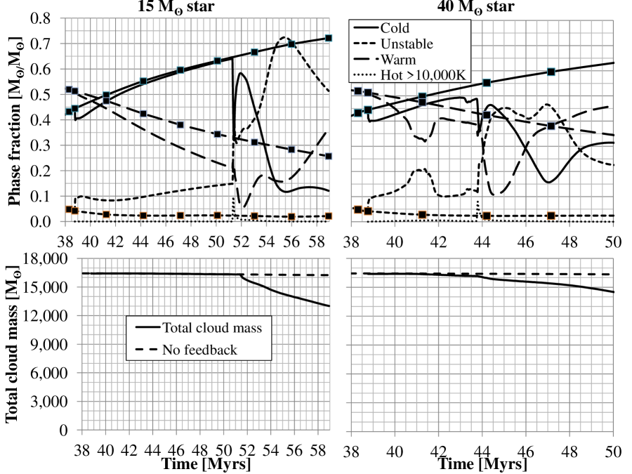
Figure 13: Phase fraction and total cloud mass for the two stellar feedback simulations. The reference case without feedback is indicated by lines with markers in the phase fraction plots and dashed lines in the total cloud mass plots.

In Fig. 13 we show the phase fraction and total cloud mass for the two feedback simulations. Prior to feedback beginning, the cloud is thermally in equilibrium with 50% of its mass in the warm phase (with temperature between 5,000 K and 10,000 K) and $\approx 45$% of its mass in the cold phase (with temperature below 160 K). The remaining 5% is in the unstable equilibrium part of the pressure-density phase-space between 160 K and 5,000 K. Once mechanical feedback starts, the hot shocked gas moves out of thermal equilbrium and takes a cooling time to radiate away its excess energy. The low density shocked stellar wind gas has a comparatively long cooling timescale, while the denser and cooler swept-up gas has a much shorter cooling timescale. Similarly, the hot SN ejecta and the gas it sweeps up have comparatively long cooling timescales (see also the earlier discussion in Section 4.1).

Fig. 13 shows that during the wind phase of the 15 M_⊙ star case, the fraction of cold material increases very much like the reference case with no feedback - the cloud continues to form. However, the introduction of stellar feedback has caused the amount of warm thermally stable material to decrease as compared to the reference case. The temperature of this material has presumably been increased by the compacting and pressurising effect of the stellar wind, thereby changing it back into the thermally unstable state (between 160 K and 5,000 K). The presence of a larger quantity of unstable material as compared to the reference case enables the condensation of more cold material, allowing the fraction of cold material to return to the level without feedback.

Since the 15 M_⊙ star only introduces a few solar masses of material during the wind phase, the total cloud mass barely changes until the SN. The SN then launches hundreds and eventually thousands of solar masses of material out of the cloud (as seen in the bottom left panel of Fig. 13). The SN rapidly heats nearly 10% of the cloud material into the hot thermal phase (above 10,000 K), but the majority of this material radiatively cools quickly and the fraction of hot material drops back close to zero before the SNR leaves the grid (at 51.6 Myrs as noted in Section 4.1). The amount of cold material decreases very rapidly post-SN, returns to a high fraction of 0.58 after 0.5 Myrs - the point at which the SN forward shock has progressed through the cloud - and then decreases as the remnant evolves. These changes can be understood as the sweeping up and ejection of diffuse material from the cloud by the SN, whilst the cold filamentary material reacts much more slowly. Some of this behaviour may also be due to the (SN) shock heating and subsequent cooling of dense material, as found by Rogers & Pittard (2013).

Eventually though, the cold dense material is stripped out of the cloud. This reduction in dense cold material is matched by an increase in lower density unstable material, indicating the disruption of the cloud by the SN. At 4 Myrs post-SN, around 55 Myrs into the evolution of the cloud, the fraction of unstable material peaks.

At this time only $\sim$15% of the cold phase cloud remains. However, 85% of the total cloud mass remains on the grid. Thus the majority of the mass remains in the cloud, though now mostly in the thermally unstable phase. Some cold material does survive the SN, and there is evidence for a slight increase 6 Myrs post-SN. However, this result is at the limit of applicability of these simulations, as numerical issues are present due to the forward SN shock having long since passed off the grid. Confirming an increase in cold cloud material - or in other words new cloud formation - requires further study.

To summarize, for the 15 M_⊙ star case, the wind phase has very little effect on the cold cloud material - there is little variation in the cold phase fraction compared with the ‘no feedback’ case. It is only after the SN that the cloud is strongly dissipated.

In the 40 M_⊙ star case, the fraction of cold material is initially reduced by the injection of the stellar wind but then gradually rises until the late stages of the star’s evolution, when the large effect of the stellar wind has led to considerable differences as compared to the no feedback case. During the time taken to establish the tunnel through the cloud, between the initial formation of the star at 38.8 Myrs, and the time when the wind bubble reaches the grid boundaries at $\approx 41$ Myrs, the structural changes driven by the stellar wind significantly affect the diffuse parts of the parent cloud. Once the wind tunnel through the cloud has been firmly established (from $\approx 42$ Myrs to the SN explosion at 43.7 Myrs), the fraction of cloud material in the unstable phase is roughly constant, whilst the warm and cold material fractions change. The fact that the rates of change of the fractions of warm and cold material match the ‘no feedback’ case indicate that this is due to continuing cloud evolution in the parts of the cloud that are relatively unaffected by the stellar wind. The total mass of the cloud slowly reduces, especially once the tunnel has become established, as the flow through the tunnel entrains some of the cloud material from the tunnel walls and carries it off the simulation grid.

The behaviour at and after the SN is similar to the 15 M_⊙ case albeit with less extreme fractional changes, in accordance with a significant part of the SN energy leaving the grid along the wind tunnel. After a similarly short period, the hot phase material has cooled and the hot fraction has returned to zero. After 3.5 Myrs post-SN, the cold and warm fractions again rise, with material moving out of the unstable phase. However, since the grid boundaries may have affected these results this observation should again be treated with caution and requires further investigation.

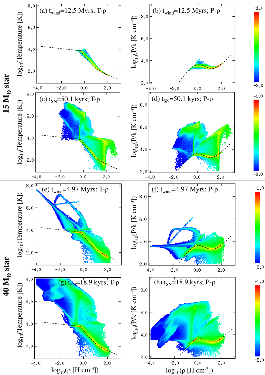
Figure 14: Mass-weighted phase space probability distributions for the two simulations presented here at different times during the stellar evolution. Over-plotted dashed lines indicate the approximate thermal equilibrium between heating and cooling prescriptions used herein.

In Fig. 14 we plot the temperature-density (in the left column) and pressure-density (in the right column) distributions for the two cases considered in this work using 200 bins in log density and 200 bins in log temperature/pressure. We also over-plot the approximate thermal equilibrium curve for the heating and cooling prescriptions used in this work. In the first row, we show the distributions at the end of the wind phase for the case of the 15 M_⊙ star. Most of the material remains in thermal equilibrium, tracing the equilibrium curve. Two distinct stable phases (warm and cold) are in approximate pressure equilibrium with each other.

In the second row, we show the distributions 50 kyrs after the SN. Towards the upper left of each distribution is the low density, hot phase, which consists of SN shock heated gas. It is not yet in pressure equilibrium with the warm phase, but evolves towards this equilibrium as the simulation progresses beyond that shown here. The distribution at low density is reasonably wide in pressure and temperature. The reason for this is the presence of both shock heated and adiabatically cooled gas, as noted in a similar analysis of such distributions influenced by feedback simulated by Walch et al. (2015). The SN has also shock-heated an appreciable amount of the cold dense material, spreading the distribution upwards at high density in both plots.

In the third row of Fig. 14, we show the distributions for the case of the 40 M_⊙ star at the end of the wind phase. The distributions are considerably different to the lower mass star case. The two distinct stable cloud phases are still present in thermal equilibrium, but are now accompanied by the low density tunnel indicated by the branch stretching away from the equilibrium curve horizontally to the left at the same P/k$\sim 10^{3.5}$ K cm^-3 in the pressure-density distribution. The ”bubble within a bubble” that is the wind-blown shell around the star that formed during the last stages of stellar evolution is responsible for the branch and arc of material out of equilibrium at higher pressure. Specifically, the diagonal line that spans from (P,$\rho$)=($10^{6}$,$10^{-1}$) down to connect to the tunnel branch at (P,$\rho$)=($10^{3.5}$,$10^{-2.75}$) is the wind injection region and region of undisturbed wind material up to the reverse shock. The reverse shock is indicated by the jump back up in pressure to the over-pressured (with respect to the cloud and tunnel) “bubble within a bubble” that is itself indicated by the horizontal branch at P/k$\sim 10^{5}$ K cm^-3 that arcs back to the equilibrium curve. The greater power of the wind has also driven a broadening of the distributions, with heated material above the equilibrium curve radiatively cooling towards the equilibrium curve. Cooling by expansion has led to low density, cool gas below the equilibrium curve.

Similarly to the 15 M_⊙ star case, the SN event has created a low-density, hot phase in the upper left of the distribution and this hot gas component is considerably more pronounced (the younger age of the remnant in the 40 M_⊙ star case means that the maximum temperature and pressure on the grid is higher). Unlike the previous case though, the SN has had far less effect on the cold material. Only late post-SN is there any sign that the SN has heated the dense material, with less of an effect than the previous case. Eventually, the hot gas pressure adjusts to the local pressure of the cloud, as is expected on larger scales for a given galaxy following the effect of supernovae (Ostriker, McKee & Leroy, 2010), again lending credibility to our simulations.

4.4 Mixing

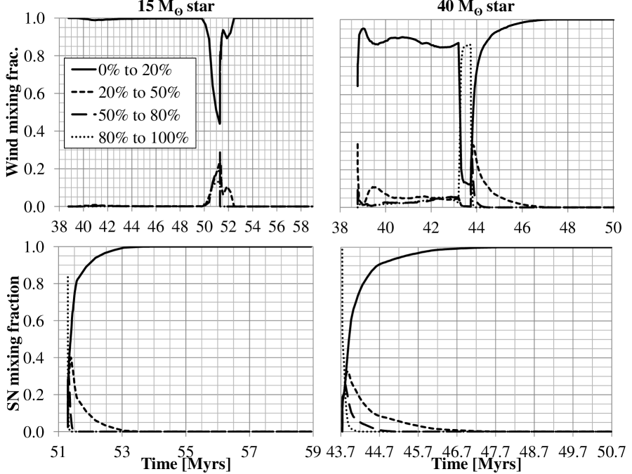
Figure 15: Levels of mixing of the wind material (top) and SN material (bottom) with the cloud material throughout the stellar feedback simulations. A value of 100% indicates no mixing of the wind/SN material with the cloud material.

In Fig. 15 we show the mixing of the stellar wind material (on the top row) and the SN material (on the bottom row) with cloud material. In the 15 M_⊙ star case, wind material is immediately well mixed, since it is all at fractions of no higher than 20% with respect to the cloud material. Whilst an equivalent amount of mass was taken out of the injection region to make the star, some cloud material remained in the injection region. The weakness of the wind implies that even in the very initial stages of switching on the wind, there is no brief period when the injection region is almost entirely wind material i.e. there is no transition observed from “no mixing” (at 100%) down to well mixed. Only during the late phases of evolution is the slow dense wind not completely mixed (though most of it still is). The subsequent SN then mixes well both the wind and SN material with the cloud material. This is perhaps not surprising as neither the stellar wind, nor the SN, inject large amounts of material. Therefore, it can be concluded that mixing is very efficient for both the wind and the SN associated with the 15 M_⊙ star.

Fig. 15 also shows that the stellar wind of the 40 M_⊙ star is not as well mixed as that of the 15 M_⊙ star. In this case, the brief initial period of mixing down from almost 100% in the injection region is indicated by the sharp initial transience. Approximately 90% of it is mixing down to less than 20% fraction of the material in a cell, but a non-zero fraction does not mix below 80% stellar wind material. This is the material which stays in the wind tunnel and escapes the grid along the tunnel. Again reflecting the isolating effect of the tunnel, this time between the SN and cloud material, the SN material takes far longer to mix with the cloud material than in the 15 M_⊙ star case. However, over time, the wind and SN material post-SN gradually mix more completely with the cloud material. Mixing for both the 15 M_⊙ star case and the 40 M_⊙ star case would appear to be efficient in these simulations.

For these simulations, we have not quantitatively examined the nature of the material leaving the grid. The wind tunnel in the 40 M_⊙ star case does not allow for as efficient entrainment of cloud material off the grid, but in both cases the SN drives material out of the cloud, as investigations of the phase fractions of material have shown in the previous section. Further investigations may shed more light on mass-loading and the entrainment of material leaving the grid. We will examine this in a future work.

5 Comparisons to previous work and observations

5.1 Comparisons to previous work

It is not immediately straight forward to compare the present work with our previous efforts (Rogers & Pittard, 2013, 2014) due to the large differences in initial conditions. However, there are certainly some key differences, such as the way that wind energy is transferred to the wider surroundings (through a multitude of porous channels in Rogers & Pittard (2013) compared to the expansion of a coherent bubble in the present work). There are also similarities, such as the ability of SNe to transport large amounts of energy without strongly affecting the parent cloud (at least not quickly). In both works the key factor in this respect is the shaping effect of the pre-SN stellar winds, which makes the cloud highly porous (Rogers & Pittard, 2013), or as in this work opens up large-scale channels which direct the SN energy.

Other work has noted how difficult it is for SN feedback alone to entirely disrupt more massive molecular clouds. For instance, Walch & Naab (2015) find that a single SN has very little impact on a $10^{5}$ M_⊙ cloud unless it explodes into a low density environment. Subsequent SNe help only if the second explosion happens during the snowplough phase of the first one. Similarly, Körtgen et al. (2016) find that single SNe disperse $\sim$10 pc-sized regions but do not disrupt entire clouds, which instead requires clustered, short-interval SNe to form large hot bubbles. Our simulations focus on feedback in a cloud of lower mass than the Walch & Naab (2015) and Körtgen et al. (2016) studies, and also include the effect of the stellar wind, so our conclusions are naturally somewhat different. In our current simulations we also find differences in the nature of the feedback in the 15 M_⊙ and 40 M_⊙ star cases, including the initial effect of the SN on the cloud, although in both cases the molecular sheet and the surrounding diffuse cloud are eventually dispersed. These differences are caused by the different structures that the SN explodes into. In the 15 M_⊙ star case the weak preceding wind barely creates a wind-blown cavity, and the molecular sheet has only a small hole in its centre. The resulting SNR sweeps up the molecular sheet but also expands into the diffuse cloud in which the molecular sheet resides (see Fig. 4). The molecular sheet is pushed back and disrupted over the following several Myr (see Fig. 7). On the other hand, in the 40 M_⊙ star case the SN explosion occurs at the centre of a large hole in the molecular sheet, and the SN ejecta initially expand almost unhindered through low density wind material (see Fig. 9). A significant part of the SNR energy then appears to be focused along the wind-blown cavity, and is carried away from the molecular cloud. Nevertheless, we find that the molecular sheet is still pushed back on Myr timescales and is eventually disrupted. Our work clearly highlights the importance of capturing the effect of the preceding stellar wind phase on the resulting SNR dynamics.

Turbulence resists the shaping effect of stellar winds. High levels of turbulence ($Mach\sim$ 2-3) have been shown (Offner & Arce, 2015; Körtgen et al., 2016) to resist and dilute the effects of winds and SN. However, questions have now arisen over the presence of such turbulent conditions in dark molecular clouds. Hacar et al. (2016) claim that the supersonic line-spreading taken to indicate supersonic turbulence in the L1517 region of the Taurus cloud is in fact misleading and at most transonic large-scale velocities are present in the small-scale dark cores, giving rise to supersonic lines through superposition of multiple transonic line velocity components separated by supersonic velocity differences. We generate transonic large-scale velocities in our model as material flows and cools onto the filamentary sheet-like cloud. Our results would indicate that structured transonic velocities do not pose a barrier to the shaping effects of stellar winds. Offner & Arce (2015) also found that stellar mass-loss rates must be greater than 10^-7 M_⊙ yr^-1 in order to reproduce shell properties. In the 15 M_⊙ star case we have considered, mass-loss rates are less than this limit for the entire MS evolution of the star, rising from 10^-8 M_⊙ yr^-1 to only 10^-7.4 M_⊙ yr^-1. On the other hand, the 40 M_⊙ star always has a mass-loss rate above this limit - during its MS evolution it loses mass at between 10^-6.4 and 10^-6 M_⊙ yr^-1. Our results, albeit testing only these two cases, appear to be in agreement with the Offner & Arce result - the wind from the 15 M_⊙ has little effect on its parent cloud, restricted to a few pc radius in the corrugated sheet of the cloud. In contrast, the wind from the 40 M_⊙ star evacuates a large tunnel-like cavity through the cloud, strongly affecting the parent molecular cloud within a $\sim$20 pc radius of the star’s location.

5.2 Bubbles Interacting With Flattened Clouds and Bipolar HII regions

Observations of wind-blown-bubbles often reveal that the surrounding cold gas has a ring-like, rather than a spherical, morphology (Beaumont & Williams, 2010; Deharveng et al., 2010). These observations detect little CO emission towards the bubble centres, with the implication that the molecular clouds which the bubbles are embedded in have thicknesses of only a few parsecs. The current work is highly relevant to such observations. For instance, Fig. 8 shows that when a massive star is located in a relatively thin sheet the bubble that forms initially has a bipolar structure and a ring of swept-up material forms within the sheet. If the magnetic field in the surrounding medium is perpendicular to the sheet the out-flowing wind material is then directed along the field lines and flows perpendicular to the molecular sheet. Although we have not included photoionization in our simulations, we expect that a bipolar HII region would have formed if we had (see, e.g., Bodenheimer et al., 1979; Deharveng et al., 2015). A detailed comparison to such observations is clearly warranted.

6 Summary and conclusions

In this work we have explored the effects of mechanical stellar wind and supernova (SN) feedback on realistic molecular clouds in magnetic and thermal pressure equilibrium. Our initial condition has been based on the work of Wareing et al. (2016) in which a diffuse atomic cloud was allowed to form structure through the action of the thermal instability, under the influence of gravity and magnetic fields, but without injected turbulence. The resulting structure is best described as a corrugated molecular sheet surrounded by a diffuse atomic cloud. The molecular sheet appears filamentary in projection. Once densities in the sheet had reached 100 cm^-3, a single massive star was introduced at the highest density location after a further gravitational free-fall time of $\sim$5 Myrs. We considered two cases: formation of a 15 M_⊙ star or a 40 M_⊙ star. Their stellar winds (based on realistic Geneva stellar evolution models) subsequently affect the parent cloud, and at the end of each star’s life a SN explosion is modelled.

In the 15 M_⊙ star case the stellar wind has very little effect on the molecular cloud, forming only a small bipolar cavity. The SN is virtually oblivious to the wind cavity: instead, it is primarily shaped by the presence of the molecular sheet and the magnetic field which threads the cloud. The SN strongly affects the sheet-like molecular cloud and its diffuse atomic surroundings. The remnant sweeps up molecular material, creating a ring in the sheet. In the diffuse cloud the remnant achieves a somewhat bipolar morphology. The interaction between the remnant and the molecular sheet results in material in the sheet being ablated into the SN remnant. The ablated material is comparatively hot and dense and hence likely to radiate strongly enough to be observable. Additional simulations at higher resolution show that high densities are achieved in the molecular sheet where ablation is taking place, raising the possibility of SN-triggered star formation, and also convince us that we are resolving the cooling in these simulations accurately.

The SNR also temporarily raises the initial magnetic field strength by a factor of 10 (in line with observations of molecular clouds that show strong magnetic fields). Field strengths four times greater than the initial field strength persist for hundreds of thousands of years. At late time (6 Myrs) the SN has largely dispersed the molecular cloud into multiple fragments, with some evidence for the formation of further cold cloud material after the SN caused material to become thermally unstable again. However, the domain size affects the simulations once the SNR shock reaches the grid boundary, so interpretation of results past this point must be treated with care.

In contrast, in the 40 M_⊙ star case, the stellar wind has a significant effect on the molecular cloud, forming a large tunnel-like cavity through the centre of the corrugated-sheet-like molecular cloud. In this case, the stellar wind also affects the magnetic field, initially increasing field strengths by factors of three or more, after which they return to close to their initial values. At the end of the main sequence, the star enters the Luminous Blue Variable (LBV) and then Wolf-Rayet (WR) phases of stellar evolution. The result at the end of the WR phase is a dense shell of mostly LBV material which has been swept up by the faster WR wind. This structure is nearly spherical and has a diameter of $\sim$25 pc at the moment the star explodes as a SN. Once the SNR has swept up the LBV/WR shell, the forward shock rapidly progresses along the tunnel-like cavity, directing significant energy away from the sheet-like molecular cloud. The initial impact of the SN on the molecular sheet is also reduced by the additional distance at which the sheet lies from the explosion site.

It can be concluded from this work that SNe from the lower mass end of the range of stars undergoing core-collapse have an equally important, if not greater effect, on their parent molecular cloud than higher-mass stars, on an individual star by star basis. The weakened forward SN shock in the 40 M_⊙ star case continues to expand into the molecular cloud and diffuse cloud, but has less of an effect on it as it cools into the radiative phase of its evolution, and its shell breaks up through Rayleigh-Taylor instabilities after 500 kyrs. Again, at late time, the molecular cloud is completely disrupted. Cold cloud material still exists in the simulations, indicating cloud remnants are still present, but there is no structural resemblance to the corrugated sheet-like nature of the initial condition. There is evidence that both stars cause stable material to return to the thermally unstable phase after the SN and in the 40 M_⊙ star case, the amount of cold, dense material shows a sharp increase 3 Myrs post-SN. However, since boundary effects may be influencing our results at this time further numerical work is required to consider this late part of the cloud evolution more accurately.

Similarities exist between the stellar wind bubble in the 40 M_⊙ star case and the rings and bubbles seen in some observations (Beaumont & Williams, 2010; Deharveng et al., 2010). Our work is also relevant to understanding structures created by a cluster of young massive stars, such as the Rosette Nebula, and even to understanding bipolar HII regions (e.g. Deharveng et al., 2015). Further work is required to explore these similarities and to directly compare detailed models to the wealth of relevant observational data.

It should also be noted in this work that we have taken a single initial condition, realistic but formed from the action of the thermal instability. Different initial conditions could lead to considerably different conclusions, the key parameters being the amount of mass and degree of inhomogeneity of the parent molecular cloud, and the pressure, density and magnetic field strength of the environment. Molecular cloud masses in the Milky Way reach 10^5-6 M_⊙, considerably more than the 17,000 M_⊙ of material in the cloud investigated here. The nature and distribution of this material is key to how the stellar winds and SN affect the molecular cloud. In future work we will explore further how these parameters affect the resistance of molecular clouds to winds, supernovae, and ionising radiation.

Appendix A Line profiles

Figure 16: Line profiles of the wind-cloud structure shown in Figure 3 for the 15 M_⊙ star simulation. Left column: profiles along the magnetic field in the $x$ direction at the location of the central star ($y$,$z$) = (0.0, 0.0125). Right column: profiles across the magnetic field in the $z$ direction and across the corrugated sheet of the molecular cloud at the location of the central star ($x$,$y$) = (-0.025, 0.0).

References

- Agertz et al. (2013) Agertz O., Kravtsov A. V., Leitner S., Gnedin N. Y., 2013, ApJ, 770, 25
- Anderson et al. (2011) Anderson L. D., Bania T. M., Balser D. S., Rood R. T., 2011, ApJSS, 194, 32
- Beaumont & Williams (2010) Beaumont C. N., Williams J. P., 2010, ApJ, 709, 791
- Beuther, Linz & Henning (2008) Beuther H., Linz H., Henning T., eds, 2008, ASp Conf. Ser. Vol. 387. Massive Star Formation: Observations Confront Theory. Astron. SOc. Pac., San Francisco
- Blondin et al. (1998) Blondin J. M., Wright E. B., Borkowski K. J., Reynolds S. P., 1998, ApJ, 500, 342
- Bodenheimer et al. (1979) Bodenheimer P., Tenorio-Tagle G., Yorke H. W., 1979, ApJ, 233, 85
- Dale & Bonnell (2011) Dale J. E., Bonnell I. A., 2011, MNRAS, 414, 321
- Dale, Ercolano & Bonnell (2012) Dale J. E., Ercolano B., Bonnell I. A., 2012, MNRAS, 424, 377
- Dale et al. (2014) Dale J. E., Ngoumou J., Ercolano B., Bonnell I. A., 2014, MNRAS, 442, 694
- Dale, Ercolano & Bonnell (2015) Dale J. E., Ercolano B., Bonnell I. A., 2015, MNRAS, 451, 987
- Dedner et al. (2002) Dedner A., Kemm F., Kröner D., Munz C.-D., Schnitzer T., Wesenberg M., 2002, J. Comput. Phys., 175, 645
- Deharveng et al. (2010) Deharveng L., et al., 2010, A&A, 523, A6
- Deharveng et al. (2015) Deharveng L., et al., 2015, A&A, 582, A1
- Dyson (1994) Dyson J. E., 1994, Lecture Notes Phys., 431, 93
- Ekström et al. (2012) Ekström S., et al. 2012, A&A, 537, id.A146
- Everett & Churchwell (2010) Everett J. E., Churchwell E., 2010, ApJ, 713, 592
- Fall, Krumholz & Matzner (2010) Fall S. M., Krumholz M. R., Matzner C. D., 2010, ApJ, 710, L142
- Falle (1991) Falle S. A. E. G., 1991, MNRAS, 250, 581
- Falle (2005) Falle S. A. E. G., 2005, Proceedings of the Chicago Workshop on Adaptive Mesh Refinement Methods, Springer Lecture Notes in Computational Science and Engineering (Springer, New York, USA), 41, 235
- Field (1965) Field G. B., 1965, ApJ, 142, 531
- Fierlinger et al. (2016) Fierlinger K. M., Burkert A., Ntormousi E., Fierlinger P., Schartmann M., Ballone A., Krause M. G. H., Diehl R., 2016, MNRAS, 456, 710
- Fogerty et al. (2016) Fogarty E., Frank A., Heitsch F., Carroll-Nellenback J., Haig C., Adams M., MNRAS submitted, arXiv:1602.01417v1
- Gatto et al. (2015) Gatto A., et al. 2015, MNRAS, 449, 1057
- Georgy et al. (2015) Georgy C., Ekström S., Hirschi R., Meynet G., Groh J., Eggenberger P., 2015, in ”Wolf-Rayet Stars: Proceedings of an International Workshop” held in Potsdam, Germany, 1-5 June 2015 (Eds. Haimann W.-R., Sander A., Todt H.), published by Universitätsverlag Potsdam, pp. 229-232. arXiv: 1508.04650
- Girichidis et al. (2015) Girichidis P., et al. 2015, MNRAS, accepted, arXiv: 1508.06646
- Gnat & Ferland (2012) Gnat O., Ferland G. J., 2012, ApJS, 199, article id. 20
- Godunov (1959) Godunov S. K., 1959, Mat. Sbornik 47, 271
- Gray & Scannapieco (2011) Gray W. J., Scannapieco E., 2011, ApJ, 733, 88
- Hacar et al. (2016) Hacar A., Alves J., Burkert A., Goldsmith P., 2016 A&A accepted, arXiv:1603.08521v1
- Harper-Clark & Murray (2009) Harper-Clark E., Murray N., 2009, ApJ, 693, 1696
- Heitsch et al. (2005) Heitsch F., Burkert A., Hartmann L. W., Slyz A. D., Devriendt J. E. G., 2005, ApJ, 633, L113
- Kim & Ostriker (2015) Kim C.-G., Ostriker E. C., 2015, ApJ, 802, 99
- Koenig et al. (2012) Koenig X. P., Leisawitz D. T., Benford D. J., Rebull L. M., Padgett D. L., Assef R. J., 2012, ApJ, 744, 130
- Körtgen (2015) Körtgen B., 2015, PhD Thesis, Fachbereich Physik der Universität Hamburg
- Körtgen et al. (2016) Körtgen B., Seifried D., Banerjee R., Vázquez-Semadeni E., Zamora-Avilés M., 2016, MNRAS, 459, 3460
- Koyama & Inutsuka (2000) Koyama H., Inutsuka S.-I., 2000, ApJ, 532, 980
- Koyama & Inutsuka (2002) Koyama H., Inutsuka S.-I., 2002, ApJ, 564, L97
- Krumholz & Matzner (2009) Krumholz M. R., Matzner C. D., 2009, ApJ, 703, 1352
- Krumholz & Thompson (2012) Krumholz M. R., Thompson T. A., 2012, ApJ, 760, 155
- Kurganov & Tadmor (2000) Kurganov A., Tadmor E., 2000, J. Co. Ph., 160, 241
- Lopez et al. (2011) Lopez L. A., Krumholz M. R., Bolatto A. D., Prochaska J. X., Ramirez-Ruiz E., 2011, ApJ, 731, 91
- Lopez et al. (2014) Lopez L. A., Krumholz M. R., Bolatto A. D., Prochaska J. X., Ramirez-Ruiz E., Castro D., 2014, ApJ, 795, 121
- Martizzi, Faucher-Giguère & Quataert (2015) Martizzi D., Faucher-Giguère C.-A., Quataert F., 2015, MNRAS, 450, 504
- Meaburn et al. (1988) Meaburn J., Dyson J. E., Hartquist T. W., 1988, MNRAS, 230, 243
- Menon (1962) Menon T. K., 1962, ApJ, 135, 394
- Murray, Quataert & Thompson (2010) Murray N., Quataert E., Thompson T., 2010, ApJ, 709, 191
- Offner & Arce (2015) Offner S. S. R., Arce H. G., 2015, ApJ, 811, article i.d. 146
- Ostriker, McKee & Leroy (2010) Ostriker E. C., McKee C. F., Leroy A. K., 2010, ApJ, 721, 975
- Parker (1953) Parker E. N., 1953, ApJ, 117, 431
- Pellegrini et al. (2011) Pellegrini E. W., Baldwin J. A., Ferland G. J., 2011, ApJ, 738, 34
- Pittard et al. (2001a) Pittard J. M., Dyson J. E., Hartquist T. W., 2001a, A&A, 367, 1000
- Pittard et al. (2001b) Pittard J. M., Hartquist T. W., Dyson J. E., 2001b, A&A, 373, 1043
- Pittard et al. (2010) Pittard J. M., Hartquist T. W., Falle S. A. E. G., 2010, MNRAS, 405, 821
- Rogers & Pittard (2013) Rogers H., Pittard J. M., 2013, MNRAS, 431, 1337
- Rogers & Pittard (2014) Rogers H., Pittard J. M., 2014, MNRAS, 441, 964
- Sharma et al. (2014) Sharma P., Roy A., Nath B. B., Shchekinov Y., 2014, MNRAS, 443, 3463
- Silich, Tenorio-Tagle & Rodríguez-González (2004) Silich S., Tenorio-Tagle G., Rodríguez-González A., 2004, ApJ, 610, 226
- Simpson et al. (2016) Simpson C.M., Pakmor R., Marinacci F., Pfrommer C., Springel V., Glover S.C.O., Clark P.C., Smith R.J., 2016, ApJL, 827, article i.d. L29
- Truelove et al. (1997) Truelove J.K., Klein R.I., McKee C.F., et al. 1997, ApJ, 489, L179
- Van Loo, Butler & Tan (2013) Van Loo S., Butler M.J., Tan J.C., 2013, ApJ, 764, 36
- Van Loo et al. (2014) Van Loo S., Keto E., Zhang Q., 2014, ApJ, 789, article id. 37
- Van Loo et al. (2015) Van Loo S., Tan J. C., Falle S. A. E. G., 2015, ApJL, 800, article id. L11
- Vázquez-Semadini et al. (2006) Vázquez-Semadini E., Ryu D., Passot T., González R. F., Gazol A., 2006, ApJ, 643, 245
- Vázquez-Semadini et al. (2007) Vázquez-Semadini E., Gómez G.C., Jappsen A. J., Ballasteros-Paredes J., González R. F., Klessen R. S., 2007, ApJ, 657, 870
- Vázquez-Semadini et al. (2008) Vázquez-Semadini E., González R. F., Ballesteros-Paredes J., Gazol A., Kim J., 2008, MNRAS, 390, 769
- Vink et al. (2000) Vink J. et al. 2000, A&A, 362, 295
- Vink et al. (2001) Vink J. et al. 2001, A&A, 369, 574
- VisIt Collaboration (2012) VisIt Collaboration, 2012, in “High Performance Visualisation – Enabling Extreme-Scale Scientific Insight”, pp. 357-372
- Walch et al. (2012) Walch S. K., Whitworth A. P., Bisbas T., Wünsch R., Hubber D., 2012, MNRAS, 427, 625
- Walch & Naab (2015) Walch S. K., Naab T., 2015, MNRAS, 451, 2757
- Walch et al. (2015) Walch S. K., et al. 2015, MNRAS, 454, 238
- Wareing et al. (2016) Wareing C. J., Pittard J. M., Falle S. A. E. G., Van Loo S., 2016, MNRAS, 459, 1803