Classical and quantum Brownian motion in an electromagnetic field FQMT15

Abstract

The dynamics of a Brownian particle in a constant magnetic field and time-dependent electric field is studied in the limit of white noise, using a Langevin approach for the classical problem and the path-integral Feynman-Vernon and Caldeira-Leggett framework for the quantum problem. We study the time evolution in configuration space of the probability distribution of an initial pure state represented by an asymmetrical Gaussian wave function and show that it can be described as the superposition of (a) the classical motion of the center of mass, (b) a rotation around the mean position, and (c) a spreading processes along the principal axes.

I Introduction

The problem of a Brownian particle in a magnetic field arises in different fields from condensed-matter (e.g. the Hall effect) to cosmology (e.g. cosmic rays). The present paper focuses on Brownian motion in a constant magnetic field and a spatially homogeneous, possibly time-dependent) electromagnetic field, a problem studied so far by various authors both in the classical regime Taylor1961a ; Kursunoglu1962a ; Kursunoglu1963a ; Liboff1966a ; Karmeshu1973a ; Karmeshu1974a ; Xiang1993a ; Singh1996a ; Lemons1999a ; Czopnik2001a ; Czopnik2001b ; Dodin2005a ; Simoes2005a ; Jimenez2006a ; Jimenez2007a ; Jimenez2008c ; Paraan2008a ; Voropajeva2008a ; Hou2009a ; Dattagupta2010a ; Lagos2011a ; Dattagupta2014a ; Friz2015a and in the quantum regime Furuse1970a ; Das1981a ; Das1982a ; Jayannavar1981a ; Marathe1989a ; Dattagupta1996a ; Mitra2010a ; Xiang1993a ; Dattagupta2010a ; Dattagupta2014a .

In the absence of noise and dissipation, a close analogy links a particle in a constant magnetic field to the harmonic oscillator, both in the classical Landau2 and in the quantum Landau3 problem. At a classical level, the particle performs periodic harmonic motion with frequency $\omega$, with $\omega=\sqrt{k/m}$ for a harmonic oscillator of mass $m$ and elastic constant $k$ and with the cyclotron frequency $\omega=|q\boldsymbol{B}|/mc$ for a particle of charge $q$ in a magnetic field $\boldsymbol{B}$ ($c$ is the speed of light). At a quantum level, the energy spectrum of both systems has equidistant energy levels $E_{n}$ with energy spacing $\Delta E=E_{n+1}-E_{n}=\hbar\omega$. However, an arbitrary small internal noise breaks this analogy and turns the harmonic-like motion of a particle in a magnetic field into one similar to that of a free Brownian particle, see Refs. Taylor1961a ; Kursunoglu1962a ; Singh1996a ; Karmeshu1974a ; Czopnik2001a for the classical case and Refs. Marathe1989a ; Li1990a ; Dattagupta1996a for the quantum case. In this paper we study the time evolution of the probability density in configuration space of a Brownian particle in a constant magnetic field and a homogeneous electric field, in the white noise approximation. We outline the main steps in the derivation of the results — further details will be presented elsewhere. For the quantum problem, the time evolution of an asymmetrical Gaussian wave packet is worked out within the framework of the Feynman-Vernon Feynman1963a and Caldeira-Leggett Caldeira1983a models.

II Classical problem

In the Langevin approach a classical Brownian particle in an electromagnetic field is described (in the limit of white noise) by the following stochastic equation Singh1996a ,

$$m\frac{d\boldsymbol{v}}{dt}=q\boldsymbol{E}+\frac{q}{c}\boldsymbol{v}\times\boldsymbol{B}-m\gamma\boldsymbol{v}+\boldsymbol{R}(t)\ .$$ (1)

Here $\boldsymbol{v}(t)=(v_{x}(t),v_{y}(t),v_{z}(t))=d\boldsymbol{r}(t)/dt$ is the particle velocity at time $t$; $\boldsymbol{r}(t)=(x(t),y(t),z(t))$ is the particle position; the first two terms on the right hand side are the electric and the Lorentz force, respectively; the last two terms represent the environment forces, i.e., the dissipative force $-m\gamma\boldsymbol{v}$ ($\gamma$ is the friction coefficient) and the random force $\boldsymbol{R}(t)=(R_{x}(t),R_{y}(t),R_{z}(t))$, assumed as a Gaussian zero-mean $\delta$-correlated stochastic process ($i,j=x,y,z,$),

$$\left\langle R_{i}(t)\right\rangle=0\ ,~{}~{}~{}\left\langle R_{i}(t)R_{j}(s)\right\rangle=\frac{2m\gamma}{\beta}\delta(t-s)\delta_{ij},$$ (2)

where $\beta=1/k_{B}T$ is the inverse temperature and $\left\langle\dots\right\rangle$ represents a statistical averaging over the stochastic force configurations.

Decomposing the velocity $\boldsymbol{v}=\boldsymbol{v}_{\parallel}+\boldsymbol{v}_{\perp}$, with $\boldsymbol{v}_{\parallel}$ parallel and $\boldsymbol{v}_{\perp}$ perpendicular to the magnetic field, and analogously for the electric field, $\boldsymbol{E}=\boldsymbol{E}_{\parallel}+\boldsymbol{E}_{\perp}$, and the random force, $\boldsymbol{R}=\boldsymbol{R}_{\parallel}+\boldsymbol{R}_{\perp}$, Eq. (1)becomes decoupled,

$$m\frac{d\boldsymbol{v}_{\parallel}}{dt} = q\boldsymbol{E}_{\parallel}-m\gamma\boldsymbol{v}_{\parallel}+\boldsymbol{R}_{\parallel}(t)\,,$$ (3)

$$m\frac{d\boldsymbol{v}_{\perp}}{dt} = q\boldsymbol{E}_{\perp}+\frac{q}{c}\boldsymbol{v}_{\perp}\times\boldsymbol{B}-m\gamma\boldsymbol{v}_{\perp}+\boldsymbol{R}_{\perp}(t)\,.$$ (4)

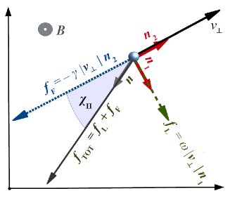
Figure 1: Lorentz force $f_{\mathrm{L}}$, friction force $f_{\mathrm{F}}$, and resulting generalized friction force $f_{\mathrm{TOT}}$ proportional to $|\boldsymbol{v}_{\perp}|$, forming a constant angle $\chi_{\mathrm{H}}$ with respect to $\boldsymbol{v}_{\perp}$; see text for details.

The motion parallel to the magnetic field is equivalent to that of a one-dimensional Langevin particle acted upon only by the force $q\boldsymbol{E}_{\parallel}(t)$ and will not be considered further. It is now useful to define the versors

$$\boldsymbol{n}_{2}=\frac{\boldsymbol{v}_{\perp}^{\,}}{|\boldsymbol{v}_{\perp}|^{\,}}\,,~{}~{}~{}~{}\boldsymbol{n}_{1}=\boldsymbol{n}_{2}\times\frac{\boldsymbol{B}}{|\boldsymbol{B}|}\,,$$ (5)

see Fig. 1, and rewrite Eq. (4) as

$$\frac{d\boldsymbol{v}_{\perp}}{dt}=\frac{q}{m}\boldsymbol{E}_{\perp}+(\omega\,\boldsymbol{n}_{1}-\gamma\,\boldsymbol{n}_{2})|\boldsymbol{v}_{\perp}|+\frac{1}{m}\boldsymbol{R}_{\perp}(t),~{}~{}$$

$$=\frac{q}{m}\boldsymbol{E}_{\perp}+(\sin\chi_{\mathrm{H}}\,\boldsymbol{n}_{1}\!-\!\cos\chi_{\mathrm{H}}\,\boldsymbol{n}_{2})\varGamma|\boldsymbol{v}_{\perp}|+\frac{1}{m}\boldsymbol{R}_{\perp}(t).~{}~{}$$ (6)

Here $\sin\chi_{\mathrm{H}}=\omega/\varGamma$, $\cos\chi_{\mathrm{H}}=\gamma/\varGamma$ are the force direction cosines in the $(\boldsymbol{n}_{1},\boldsymbol{n}_{2})$ frame and

$$\tan\chi_{\mathrm{H}}=\frac{\omega}{\gamma}\ ,~{}~{}~{}~{}~{}\varGamma=\sqrt{\gamma^{2}+\omega^{2}}\ ,$$ (7)

are the Hall angle Ashcroft1976a and the “effective damping constant”. Equation (6) displays the similarity between the Lorentz and the friction forces, both proportional to $|\boldsymbol{v}_{\perp}|$, merging in an effective viscous force still proportional to $|\boldsymbol{v}_{\perp}|$ with intensity $\varGamma$, forming an angle $\chi_{\mathrm{H}}$ (the Hall angle) with $\boldsymbol{v}_{\perp}$ — see Fig. 1. Note that even if $\boldsymbol{n}_{1}(t)$ and $\boldsymbol{n}_{2}(t)$ are time-dependent, $\varGamma$ and $\chi_{\mathrm{H}}$ are constant in time. The Hall angle $\chi_{\mathrm{H}}$ (known from the Hall effect Ashcroft1976a where both a magnetic and an electric field are present) measures the relative strengths of Lorentz to friction force, playing a key role also when only a magnetic field is present.

The time scales associated to $\omega$ and $\gamma$ and the parameters $\varGamma$ and $\chi_{\mathrm{H}}$ can be related to each other through the complex friction coefficient

$$\widetilde{\varGamma}=\gamma+i\omega=\varGamma\exp\left(i\chi_{\mathrm{H}}\right)\ ,$$ (8)

which is relevant both in the classical and in the quantum problem — $\gamma$ and $\omega$ represent the real and imaginary parts of $\widetilde{\varGamma}$, while the Hall angle $\chi_{\mathrm{H}}$ and the effective damping constant $\varGamma$ represent its modulus and phase, respectively.

II.1 Constant $\boldsymbol{B}$ and homogeneous $\boldsymbol{E}(t)$

We assume a homogeneous electric field $\boldsymbol{E}(t)$, an $\omega=qB/mc>0$, and a constant magnetic field,

$$\boldsymbol{B}=(0,0,B)\,.$$ (9)

It is convenient to introduce the complex coordinate Landau2

$$Z(t)=x(t)+iy(t)\ ,$$ (10)

and the complex forces $q\widetilde{E}(t)=qE_{x}(t)+iqE_{y}(t)$, $\widetilde{R}(t)=R_{x}(t)+iR_{y}(t)$. Using Eq. (1), one finds that $Z(t)$ follows the complex Langevin equation

$$m\ddot{Z}(t)=-m\widetilde{\varGamma}\dot{Z}(t)+q\widetilde{E}(t)+\widetilde{R}(t)\,.$$ (11)

Here the Lorentz and friction forces merged in the generalized friction force given by the term $-m\widetilde{\varGamma}\dot{Z}(t)$, where $\widetilde{\varGamma}$ is defined in Eqs. (7). By integrations of Eq. (11) between $t=t_{a}$ and $t=t_{b}$, one obtains the complex velocity $\dot{Z}(t_{b})$ and coordinate $Z(t_{b})$,

$$\dot{Z}(t_{b}) =\dot{Z}_{0}\exp\left(-\widetilde{\varGamma}t\right)+\frac{1}{m}\dot{F}[q\widetilde{E}+\widetilde{R}\,],~{}~{}$$ (12)

$$Z(t_{b}) =Z_{0}+\frac{\dot{Z}_{0}}{\widetilde{\varGamma}}\left[1-\exp\left(-\widetilde{\varGamma}t\right)\right]+\frac{1}{m}\!F[q\widetilde{E}+\widetilde{R}].~{}~{}$$ (13)

Here $t=t_{b}-t_{a}$, $Z_{0}=Z(t_{a})=x(t_{a})+iy(t_{a})$, $\dot{Z}_{0}=\dot{Z}(t_{a})=\dot{x}(t_{a})+i\dot{y}(t_{a})$; the functionals $F$ and $\dot{F}=dF[f]/dt_{b}$ represent the inhomogeneous contributions of $\widetilde{E}$ and $\widetilde{R}$,

$$F[\tilde{f}\,]=\frac{1}{\widetilde{\varGamma}}\int_{t_{a}}^{t_{b}}ds\,\left\{1-\exp\left[-\widetilde{\varGamma}(t_{b}-s)\right]\right\}\tilde{f}(s),$$ (14)

where $\tilde{f}\equiv q\widetilde{E}+\widetilde{R}$.

II.2 Constant magnetic field

Here we consider the particular case of zero electric field. For convenience we rewrite the initial conditions on the complex variable $Z$ as

$$Z_{0} =x_{0}+iy_{0}\ ,~{}~{}~{}~{}~{}~{}\dot{Z}_{0} =\dot{x}_{0}+i\dot{y}_{0}\equiv v_{0}\exp\left(i\varphi_{0}\right),~{}~{}$$ (15)

where $x_{0}\equiv x(t_{a})$, $\dot{x}_{0}\equiv\dot{x}(t_{a})$, and analogously for the $y$ components, and we have introduced the initial modulus $v_{0}=|\boldsymbol{v}_{0}|$ and angle $\varphi_{0}$ formed with the $x$-axis,

$$v_{0}=\sqrt{\dot{x}_{0}^{2}+\dot{y}_{0}^{2}},~{}~{}~{}~{}~{}\tan\varphi_{0}~{}=\frac{\dot{y}_{0}}{\dot{x}_{0}}\,.$$ (16)

From Eqs. (13) and (2), separating $\left\langle Z(t)\right\rangle$ into real and imaginary parts, one obtains the average coordinates,

$$\left\langle x(t)\right\rangle = x_{c}-\frac{v_{0}}{\varGamma}\exp(-\gamma t)\cos\left(\omega t-\varphi_{0}+\chi_{\mathrm{H}}\right)\ ,$$

$$\left\langle y(t)\right\rangle = y_{c}+\frac{v_{0}}{\varGamma}\exp(-\gamma t)\sin\left(\omega t-\varphi_{0}+\chi_{\mathrm{H}}\right)\ ,$$ (17)

where $t=t_{b}-t_{a}$ and $x_{c}$, $y_{c}$ are the coordinates of the position eventually approached for $t\gg\gamma^{-1}$,

$$x_{c} = \langle x(t\!\gg\!\gamma^{-1}\!)\rangle=x_{0}+\frac{v_{0}}{\varGamma}\cos(\chi_{\mathrm{H}}-\varphi_{0})\ ,$$

$$y_{c} = \langle y(t\!\gg\!\gamma^{-1}\!)\rangle=y_{0}-\frac{v_{0}}{\varGamma}\sin(\chi_{\mathrm{H}}-\varphi_{0})\ .$$ (18)

This provides a simple geometrical interpretation of the Hall angle $\chi_{\mathrm{H}}$ as the total deflection angle of the particle with respect to its initial velocity, while the effective friction coefficient $\varGamma$ defines the total distance covered by the particle, $d_{B}=[(y_{c}-y_{0})^{2}+(x_{c}-x_{0})^{2}]^{1/2}=v_{0}/\varGamma$.

In polar coordinates, choosing the origin in the asymptotic position $(x_{c},y_{c})$, from Eqs. (17) one obtains

$$r(t) =\sqrt{[\left\langle x(t)\right\rangle-x_{c}]^{2}+[\left\langle y(t)\right\rangle-y_{c}]^{2}}=\frac{v_{0}}{\varGamma}\,\mathrm{e}^{-\gamma t},$$ (19)

$$\theta(t) =\arctan\left[\frac{\left\langle y(t)\right\rangle-y_{c}}{\left\langle x(t)\right\rangle-x_{c}}\right]=\varphi_{0}-\chi_{\mathrm{H}}-\omega t\,.$$ (20)

By eliminating the time variable one finds that the shape of the trajectory is an exponential spiral,

$$r(\theta)=\frac{v_{0}}{\varGamma}\exp\left(-\frac{\theta-\varphi_{0}+\chi_{\mathrm{H}}}{\tan\chi_{\mathrm{H}}}\right)\,.$$ (21)

Notice in Eq. (19) that the particle approaches the asymptotic position $(x_{c},y_{c})$ with time scale $\gamma^{-1}$ — as in the problem without magnetic field — and, at the same time, Eq. (20) shows a uniform angular motion with angular velocity $\omega$ — as in the frictionless problem with a constant magnetic field. These complementary features are due to the fact that the Lorentz force acts perpendicularly to the particle velocity, leaving its modulus and therefore the relaxation dynamics unaffected, so that the only effect of the magnetic field is to bend the trajectory. Whereas the friction force — being anti-parallel to the particle velocity— changes the velocity modulus as if no magnetic field is present, without influencing the direction.

The position uncertainties can be expressed through the second moments

$$\left\langle\Delta x(t)^{2}\right\rangle =\left\langle[x(t)-\left\langle x(t)\right\rangle]^{2}\right\rangle\,,$$ (22)

$$\left\langle\Delta y(t)^{2}\right\rangle =\left\langle[y(t)-\left\langle y(t)\right\rangle]^{2}\right\rangle\,,$$ (23)

$$\left\langle\Delta x(t)\Delta y(t)^{\!}\right\rangle =\left\langle[x(t)\!-\!\left\langle x(t)\right\rangle]\!\times\![y(t)\!-\!\left\langle y(t)\right\rangle]\right\rangle\,,$$ (24)

where $\Delta x(t)=x(t)-\left\langle x(t)\right\rangle$ and $\Delta y(t)=y(t)-\left\langle y(t)\right\rangle$ are the $x$ and $y$ displacements, which can be computed from $\langle\Delta Z(t)^{2}\rangle$ and $\langle|\Delta Z(t)|^{2}\rangle$. One finds $\langle\Delta x(t)^{2}\rangle=\langle\Delta y(t)^{2}\rangle$ and a radial mean square displacement Singh1996a ; Williamson1968a

$$\langle\Delta r(t)^{2}\rangle=\langle\Delta x(t)^{2}\rangle+\langle\Delta y(t)^{2}\rangle=\frac{2\cos\!\chi_{\mathrm{H}}^{\ 2}}{m\beta\gamma^{2}}\bigg{\{}\,2\gamma t~{}~{}~{}$$

$$+4\cos\chi_{\mathrm{H}}\Big{[}\mathrm{e}^{-\gamma t}\!\cos(\omega t\!+\!\chi_{\mathrm{H}})\!-\!\cos\chi_{\mathrm{H}}\Big{]}\!+\!1\!-\!\mathrm{e}^{-2\gamma t}\!\bigg{\}}.~{}~{}~{}$$ (25)

For $\chi_{\mathrm{H}}\to 0$ ($B\to 0$) this expression reduces to the mean square displacement of a Langevin particle in a plane Wang1945a , while in the asymptotic limit $\gamma t\gg 1$ one obtains

$$\left\langle\Delta r^{2}\right\rangle_{t}=4D_{B}t\ ,~{}~{}~{}~{}~{}D_{B}=\frac{\gamma}{m\beta\varGamma^{2}}\equiv{\rm Re}\left(\frac{1}{m\beta\widetilde{\varGamma}}\right)\ .$$ (26)

The latter equation resembles the Einstein relation, with $1/\gamma$ replaced by (the real part of) $1/\widetilde{\varGamma}$.

II.3 Constant electromagnetic field

It is easy to show from Eq. (13) that a homogeneous electric field modifies the mean position but not the mean square displacements. The well known case of a constant electric field $\boldsymbol{E}$ with modulus $E_{0}$ and components $E_{x}=E_{0}\cos\alpha$ and $E_{y}=E_{0}\sin\alpha$ can be recovered from Eq. (17) and is characterized by an asymptotic motion with an angle $\chi_{\mathrm{H}}$ with respect to the electric field,

$$\left\langle x(t)\right\rangle=\left\langle x(t)\right\rangle_{\boldsymbol{E}=0}+qE_{0}\cos(\alpha-2\chi_{\mathrm{H}})/m\varGamma^{2},$$

$$~{}~{}~{}~{}~{}+(qE_{0})/(m\varGamma^{2})\exp(-\gamma t)\cos\left(\omega t+2\chi_{\mathrm{H}}-\alpha\right)+V_{x}t\ ,$$

$$\left\langle y(t)\right\rangle=\left\langle y(t)\right\rangle_{\boldsymbol{E}=0}+qE_{0}\sin(\alpha-2\chi_{\mathrm{H}})/m\varGamma^{2}$$

$$~{}~{}~{}~{}~{}-(qE_{0})/(m\varGamma^{2})\exp(-\gamma t)\sin\left(\omega t+2\chi_{\mathrm{H}}-\alpha\right)+V_{y}t\ ,$$ (27)

where the drift velocities $V_{x}t$ and $V_{y}t$ are given by

$$V_{x}=\frac{qE_{0}}{m\varGamma}\cos(\alpha-\chi_{\mathrm{H}})\ ,~{}~{}~{}~{}~{}~{}V_{y}=\frac{qE_{0}}{m\varGamma}\sin(\alpha-\chi_{\mathrm{H}})\ .$$ (28)

The velocity modulus is $V_{0}=qE_{0}/m\varGamma$, confirming the role of $\varGamma$ as an effective friction coefficient.

III Quantum problem

In this section we study the time evolution of a quantum wave packet between times $t_{a}$ and $t_{b}$ ($t_{a}<t_{\rm b}$).

III.1 Initial state

It is assumed that the wave function $\varPsi(x_{a},y_{a},z_{a},t_{a})$ at the initial time $t_{a}$ is known and factorized,

$$\varPsi(x_{a},y_{a},z_{a},t_{a})=\psi(x_{a},y_{a},t_{a})\times\phi(z_{a},t_{a})\ ,$$ (29)

so that the $x$-$y$ motion, on which we concentrate, is decoupled from the $z$-motion. The problem is undetermined by a phase factor due to gauge invariance, i.e., if $\psi\to\psi\times\exp[i\varLambda]$ ($\varLambda\equiv\varLambda(x,y)$ is an arbitrary function) and ${\bf A}\to{\bf A}+\nabla\varLambda$. We assume a magnetic field ${\bf B}=(0,0,B)\equiv\nabla\times{\bf A}$ coming from a vector potential

$${\bf A}=(\ (\lambda-1)By/2,\ (\lambda+1)Bx/2,\ 0\ )\ ,$$ (30)

with arbitrary gauge parameter $\lambda$. A Gaussian shape is assumed for the initial wave function in the $x$-$y$-plane,

$$\psi(x_{a},y_{a},t_{a})=\sqrt{N_{0}}\exp\bigg{[}-\frac{(x_{a}-x_{0})^{2}}{4\sigma_{x}^{2}}-\frac{(y_{a}-y_{0})^{2}}{4\sigma_{y}^{2}}$$

$$+\frac{i}{\hbar}\left(q_{x}x_{a}+q_{y}y_{a}+\frac{\mu m\omega}{2}x_{a}y_{a}\right)\bigg{]}\,,$$ (31)

associated to a Gaussian probability density,

$$P(x_{a},y_{a},t_{a})=|\psi(x_{a},y_{a},t_{a})|^{2}$$

$$=N_{0}\exp\left[-\frac{(x_{a}-x_{0})^{2}}{2\sigma_{x}^{2}}-\frac{(y_{a}-y_{0})^{2}}{2\sigma_{y}^{2}}\right].$$ (32)

Here $N_{0}=1/2\pi\sigma_{x}\sigma_{y}$ is a normalization factor, the coordinates $(x_{0},y_{0})=(\left\langle x_{a}\right\rangle,\left\langle y_{a}\right\rangle)$ are the initial average positions ($\left\langle\dots\right\rangle$ denoting in this section a quantum average), and $\sigma_{x}$, $\sigma_{y}$ are the corresponding standard deviations, $\left\langle(x_{a}-x_{0})^{2}\right\rangle=\sigma_{x}^{2}$, $\left\langle(y_{a}-y_{0})^{2}\right\rangle=\sigma_{y}^{2}$. We assumed, without loss of generality, that there is no mixed term $\propto xy$ and an anisotropic wave function with $\sigma_{x}\neq\sigma_{y}$. Finally, the parameters $q_{x}$, $q_{y}$ and $\mu$ are related to the average initial velocity $\widehat{{\bf v}}=(v_{x},v_{y})=\widehat{{\bf p}}/m=-i\nabla/m\hbar-e{\bf A}/mc$, that from Eq. (31) is

$$v_{x}=\frac{q_{x}}{m}+\frac{\mu\!-\!\lambda\!+\!1}{2}\omega y_{0},~{}v_{y}=\frac{q_{y}}{m}+\frac{\mu\!-\!\lambda\!-\!1}{2}\omega x_{0}.~{}~{}~{}$$ (33)

Note that $\widehat{{\bf v}}$ (as any other observable quantity) only depends on the difference

$$\alpha=\mu-\lambda\ ,$$ (34)

exhibiting the gauge invariance of the problem.

The quantum treatment discussed below is based on the density matrix, given at the initial time $t=t_{a}$ by

$$\rho(x_{a},y_{a},x_{a}^{\prime},y_{a}^{\prime},t_{a})=\psi(x_{a},y_{a},t_{a})\psi^{*}(x_{a}^{\prime},y_{a}^{\prime},t_{a})\ .$$ (35)

It is convenient to introduce the new coordinates

$$X=\frac{x^{\prime}\!+\!x}{2},~{}Y=\frac{y^{\prime}\!+\!y}{2},~{}\xi=\frac{x^{\prime}\!-\!x}{2},~{}\eta=\frac{y^{\prime}\!-\!y}{2},~{}~{}$$ (36)

with inverse relations $x=X-\xi/2$, $y=Y-\eta/2$, and $x^{\prime}=X+\xi/2$, $y^{\prime}=Y+\eta/2$, that are useful for simplifying calculations and because they provide a physical interpretation of the results. In terms of the new variables, the initial density matrix becomes

$$\rho(X_{a},Y_{a},\xi_{a},\eta_{a},t_{a})$$ (37)

$$= \psi\left(X_{a}-\frac{\xi_{a}}{2},Y_{a}-\frac{\eta_{a}}{2}\right)\psi^{*}\left(X_{a}+\frac{\xi_{a}}{2},Y_{a}+\frac{\eta_{a}}{2}\right)$$

$$= N_{0}\exp\bigg{\{}-\frac{(X_{a}-x_{0})^{2}}{2\sigma_{x}^{2}}-\frac{(Y_{a}-y_{0})^{2}}{2\sigma_{y}^{2}}-\frac{\xi_{a}^{2}}{8\sigma_{x}^{2}}-\frac{\eta_{a}^{2}}{8\sigma_{y}^{2}}$$

$$-\frac{i}{\hbar}\left(q_{x}\xi_{a}+q_{y}\eta_{a}+\frac{\mu m\omega}{2}\left(\xi_{a}Y_{a}+X_{a}\eta_{a}\right)\right)\bigg{\}}\ .$$

III.2 Time evolution

The reduced density matrix $\rho(X,\-Y,\-\xi,\-\eta,t)$ evolves with time in a way similar to the wave function,

$$\rho(X_{b},Y_{b},\xi_{b},\eta_{b},t_{b})$$ (38)

$$=\int dX_{a}dY_{a}d\xi_{a}d\eta_{a}J(x_{b},y_{b},t_{b}|x_{a},y_{a},t_{a})\rho(x_{a},y_{a},t_{a})\,,$$

where the effective propagator $J$ is conveniently expressed in terms of the effective action $S[X,Y,\xi,\eta]$ as

$$J(X_{b},Y_{b},\xi_{b},\eta_{b},t_{b}|X_{a},Y_{a},\xi_{a},\eta_{a},t_{a})$$

$$=\int_{a}^{\,b}\!\!DXDYD\xi D\eta\exp\left\{\frac{i}{\hbar}S[X,Y,\xi,\eta]\right\}.$$ (39)

Here $a$ represents the boundary conditions at time $t_{a}$: $X(t_{a})=X_{a}$, $Y(t_{a})=Y_{a}$, $\xi(t_{a})=\xi_{a}$, and $\eta(t_{a})=\eta_{a}$, and analogously for $b$. For an isolated system the effective action $S[X,Y,\xi,\eta]$ is the difference between the actions of the isolated system, $S[X,Y,\xi,\eta]\!=\!S_{0}[X\!-\!{1\over 2}\xi,\!Y\!-\!{1\over 2}\eta]\!-\!S_{0}[X\!+\!{1\over 2}\xi,\!Y\!+\!{1\over 2}\eta]$ — and the effective propagator factorizes in the product of two propagators for $\psi(x,y,t)$ and $\psi^{*}(x^{\prime},y^{\prime},t)$, where, for a non-relativistic particle Landau3 ,

$$S_{0}[x,y]=\int_{t_{a}}^{t_{b}}dt\left[\frac{m}{2}\left(\dot{x}^{2}+\dot{y}^{2}\right)+\frac{e}{c}\left(\dot{x}A_{x}+\dot{y}A_{y}\right)\right].$$ (40)

For a non-isolated system, the effective action contains also the influence phase $\varPhi_{2}$, coming from the integration of the environment degrees of freedom Feynman1963a ; Feynman1965a ,

$$S[X,Y,\xi,\eta] = S_{0}\left[X-\frac{\xi}{2},Y-\frac{\eta}{2}\right]-S_{0}\left[X+\frac{\xi}{2},Y+\frac{\eta}{2}\right]$$ (41)

$$+ \hbar\,\varPhi_{2}[X,Y,\xi,\eta]\ .$$

Here we focus on the dynamics of the probability density $P(X,Y,t)$ in configuration space, which is given by the diagonal elements of $\rho(x,x^{\prime},y,y^{\prime},t)$, i.e., $P(X,Y,t)=\left[\rho(x,x^{\prime},y,y^{\prime},t)\right]_{x=x^{\prime}=X;\,y=y^{\prime}=Y}$. If the coordinates $X,Y,\xi,\eta$ are used, one can obtain $P$ setting $\xi=\eta=0$, i.e., $P(X,Y,t)=\rho(X,Y,\xi=0,\eta=0,t)$. Then the probability density at time $t_{b}$, from Eqs. (39), is

$$P(X_{b},Y_{b},t_{b})=\rho(X_{b},Y_{b},0,0,t_{b})$$

$$=\int dX_{a}dY_{a}d\xi_{a}d\eta_{a}J(X_{b},Y_{b},0,0,t_{b}|X_{a},Y_{a},\xi_{a},\eta_{a},t_{a})\times$$

$$\times\rho(X_{a},Y_{a},\xi_{a},\eta_{a},t_{a})\ .$$ (42)

We now proceed to obtain $\varPhi_{2}[X,Y,\xi,\eta]$ and $J$.

III.3 Influence functional and phase

The influence phase $\varPhi$ — or equivalently the influence functional $\mathcal{F}=\exp(i\varPhi)$ — is the central quantity in the study of a non-isolated quantum system, since it describes the effect of the interaction with the environment. In the framework of the Feynman-Vernon model Feynman1963a a dissipative environment is represented in one dimension by an infinite set of harmonic oscillators interacting with the central particle. We make the simple hypothesis that the two-dimensional environment is obtained by a straightforward generalization of the one-dimensional case assuming that the central particle interacts with a set of two-dimensional oscillators, which are harmonic and isotropic in the $x$-$y$-plane.

Thus, the starting action of the total system, depending on the coordinates of the central particle $(x,y)$ and of the oscillators $\{x_{n},y_{n}\}$ ($n=1,2,\dots$) Patriarca1996a is

$$S_{\rm tot}[x,y,\{x_{n}\},\{y_{n}\}]=S_{0}[x,y]$$

$$\!+\,\frac{m}{2}\!\!\sum_{n}\!\!\int_{t_{a}}^{t_{b}}\!\!\!\!\!dt\big{\{}\dot{x}_{n}^{2}\!+\!\dot{y}_{n}^{2}\!+\!\omega_{n}^{2}\left[(x_{n}\!-\!x)^{2}\!+\!(y_{n}\!-\!y)^{2}\right]\!\!\big{\}}.$$ (43)

Notice that the oscillators have been assigned their equilibrium positions coinciding with the central particle position, as requested by general symmetry constraints Patriarca1996a . This determines both the structure of the total Lagrangian, Eq. (43), and the form of the (correlated) thermal equilibrium initial conditions — see Ref. Patriarca1996a for details. In Eq. (43), the interaction between central particle and environment oscillators factorizes into a sum of two terms for the $x$ and the $y$ dimension. Correspondingly, $x$- and $y$-factorized thermal equilibrium initial conditions at time $t=t_{a}$ are assumed for the $x$ and $y$ coordinates of the environment oscillators in the form of (one-dimensional) equilibrium density matrices at temperature $\beta^{-1}$. Within the Caldeira-Leggett model Caldeira1983a , the integration of the $x$ or $y$ environment degrees of freedom proceeds as in the 1D case Patriarca1996a and results in the influence phase

$$\varPhi_{2}[X,Y,\xi,\eta]=\varPhi_{1}[X,\xi]+\varPhi_{1}[Y,\eta]\ ,$$ (44)

(and $\mathcal{F}_{2}[X,Y,\xi,\eta]=\mathcal{F}_{1}[X,\xi]\mathcal{F}_{1}[Y,\eta]$), implying as a limit of the present model the hypothesis of dynamical and statistical independence of the $x$ and $y$ environment degrees of freedom (second properties of influence functionals Feynman1963a ). In the white noise approximation the 1D influence phase reads

$$\hbar\varPhi_{1}[X,\xi]=m\gamma\int_{t_{a}}^{t_{b}}dt\left[\xi(t)X(t)+\frac{i}{\beta\hbar}\xi^{2}(t)\right]\ .$$ (45)

Replacing $\varPhi_{1}$ and the unperturbed action (40) in Eq. (41) one obtains the effective action

$$S[X,Y,\xi,\eta]=m\int_{t_{a}}^{t_{b}}dt\bigg{[}\!-\dot{X}\dot{\xi}-\dot{Y}\dot{\eta}$$

$$+\frac{\omega(\dot{X}\eta\!+\!Y\dot{\xi}\!-\!X\dot{\eta}\!-\!\dot{Y}\xi)}{2}\!+\!\gamma(\dot{X}\xi\!+\!\dot{Y}\eta)\!+\!\frac{i\gamma(\xi^{2}\!+\!\eta^{2})}{\beta\hbar}\!\bigg{]}.~{}~{}~{}~{}~{}$$ (46)

The first two terms in the integral are the kinetic ones, the term $\propto\omega$ is due to the magnetic field, the real term $\propto\gamma$ to dissipation, and the last imaginary term to thermal fluctuations. Since this is a quadratic functional of $X(t)$, $Y(t)$, $\xi(t)$, and $\eta(t)$, then the propagator ( 39) can be calculated exactly and can be written as

$$J(X_{b},Y_{b},\xi_{b},\eta_{b},t_{b}|X_{a},Y_{a},\xi_{a},\eta_{a},t_{a})\!=\!N\!(t)\exp\!\left\{\!\frac{i\bar{S}}{\hbar}\!\right\},~{}~{}$$ (47)

where $N(t)$ is a normalization factor and $\bar{S}$ is the effective action $S$ computed along the trajectories which make it an extremum,

$$\!\!\!\frac{1}{m}\frac{\delta S}{\delta\xi(t)} = \ddot{X}(t)+\gamma\dot{X}(t)-\omega\dot{Y}(t)+\frac{2i\gamma}{\beta\hbar}\xi(t)=0,$$ (48)

$$\!\!\!\frac{1}{m}\frac{\delta S}{\delta\eta(t)} = \ddot{Y}(t)+\gamma\dot{Y}(t)+\omega\dot{X}(t)+\frac{2i\gamma}{\beta\hbar}\eta(t)=0,$$ (49)

$$\!\!\!\frac{1}{m}\frac{\delta S}{\delta X(t)} = \ddot{\xi}(t)+\gamma\dot{\xi}(t)-\omega\dot{\eta}(t)=0,$$ (50)

$$\!\!\!\frac{1}{m}\frac{\delta S}{\delta Y(t)} = \ddot{\eta}(t)+\gamma\dot{\eta}(t)+\omega\dot{\xi}(t)=0,$$ (51)

subject to the boundary conditions $a$ and $b$. The calculation is simplified by integrating by parts Eq. (46) and setting $\xi_{b}=\eta_{b}=0$ in view of the calculation of the probability density, which provides

$$\left(\bar{S}\right)_{\xi_{b}=\eta_{b}=0} = m\left[\dot{X}_{a}\xi_{a}+\dot{Y}_{a}\eta_{a}-\frac{\omega}{2}\left(Y_{a}\xi_{a}-X_{a}\eta_{a}\right)\right]$$ (52)

$$- \frac{im\gamma}{\beta\hbar}\int_{t_{a}}^{t_{b}}\!\!\!dt{\left[\xi^{2}(s)+\eta^{2}(s)\right]}_{\xi_{b}=\eta_{b}=0}.$$

Here only the solutions $\xi(t)$ and $\eta(t)$ of Eqs. (50) and (51) with final conditions $\xi_{b}=\eta_{b}=0$ are needed. In analogy with the classical case, using the coordinates $Z=X+iY$ and $\zeta=\xi+i\eta$, Eqs. (48)–(51) become

$$\ddot{Z}(t)+\widetilde{\varGamma}\dot{Z}(t)=-\frac{2i\gamma}{\beta\hbar}\zeta(t)\ ,~{}~{}~{}~{}~{}\ddot{\zeta}(t)-\widetilde{\varGamma}^{*}\dot{\zeta}(t)=0\ .$$ (53)

We skip the details that will be presented elsewhere and provide the result,

$$\left(\bar{S}\right)_{\xi_{b}=\eta_{b}=0}=m\Big{\{}\left[\mathcal{R}(t)\xi_{a}+\mathcal{I}(t)\eta_{a}\right](X_{b}-X_{a})$$

$$~{}~{}~{}~{}~{}+\left[\mathcal{R}(t)\eta_{a}-\mathcal{I}(t)\xi_{a}\right](Y_{b}-Y_{a})$$

$$~{}~{}~{}~{}~{}+\frac{\omega}{2}\left(X_{a}\eta_{a}-Y_{a}\xi_{a}\right)+\frac{2im\gamma}{\beta\hbar}\epsilon(t)\left(\xi_{a}^{2}+\eta_{a}^{2}\right)\Big{\}},~{}~{}~{}~{}~{}$$ (54)

where

$$\mathcal{R}(t)+i\mathcal{I}(t)=\frac{\widetilde{\varGamma}}{1-\exp[-\widetilde{\varGamma}t]}\,$$ (55)

$$\epsilon(t)\!=\!\frac{1}{M}\!\bigg{[}t\!+\!\frac{2\mathrm{e}^{-\gamma t}}{\varGamma}\cos(\omega t\!+\!\chi_{\mathrm{H}})\!-\!\frac{2\gamma}{\varGamma^{2}}\!+\!\frac{1\!-\!\mathrm{e}^{-2\gamma t}}{2\gamma}\bigg{]}\!,$$ (56)

$$M(t)=1-2\mathrm{e}^{-\gamma t}\cos(\omega t)+\mathrm{e}^{-2\gamma t}.$$ (57)

III.4 Probability density

The effective propagator (47), with the effective action (54), and the initial conditions (37) can be used in Eq. (42) to compute the probability density $P(X_{b},Y_{b},t_{b})$. The first two integrations give

$$P(X_{b},Y_{b},t_{b}) = f(t)\int d\xi_{a}d\eta_{a}\exp\big{(}-A_{0}\xi_{a}^{2}-B_{0}\eta_{a}^{2}$$ (58)

$$+ 2C_{0}\xi_{a}\eta_{a}+D_{0}\xi_{a}+E_{0}\eta_{a}\big{)},$$

where

$$A_{0}(t) = \frac{m^{2}}{2\hbar^{2}}\left[\sigma_{x}^{2}\mathcal{R}(t)^{2}+\sigma_{y}^{2}\mathcal{I}_{+}(t)^{2}+\frac{\hbar}{2m\sigma_{x}^{2}}+\frac{2\gamma\epsilon(t)}{m\beta}\right]\ ,$$

$$B_{0}(t) = \frac{m^{2}}{2\hbar^{2}}\left[\sigma_{y}^{2}\mathcal{R}(t)^{2}+\sigma_{x}^{2}\mathcal{I}_{-}(t)^{2}+\frac{\hbar}{2m\sigma_{y}^{2}}+\frac{2\gamma\epsilon(t)}{m\beta}\right]\ ,$$

$$C_{0}(t) = \frac{m^{2}}{2\hbar^{2}}\left[\sigma_{x}^{2}\mathcal{I}_{+}(t)^{2}-\sigma_{x}^{2}\mathcal{I}_{-}(t)^{2}+\frac{\hbar}{2m\sigma_{y}^{2}}+\frac{2\gamma\epsilon(t)}{m\beta}\right]\ ,$$

$$D_{0}(t) = \frac{im}{\hbar}\left[\mathcal{R}(t)(X_{b}-x_{0})-\mathcal{I}(t)(Y_{-}y_{0})-v_{x}\right]\ ,$$

$$E_{0}(t) = \frac{im}{\hbar}\left[\mathcal{I}(t)(X_{b}-x_{0})+\mathcal{R}(t)(Y_{b}-y_{0})-v_{y}\right]\ ,$$ (59)

where $\mathcal{I}_{\pm}(t)=\mathcal{I}(t)+\frac{1}{2}(\pm\alpha-1)\omega$ and $\alpha$ is the gauge parameter given by Eq. (34). The last integrations give

$$P(X_{b},Y_{b},t_{b}) = N(t)\exp\big{(}-A_{1}X_{b}^{2}-B_{1}Y_{b}^{2}$$ (60)

$$+ 2C_{1}X_{b}^{\prime}Y_{b}^{\prime}+D_{1}X_{b}^{\prime}+E_{1}Y_{b}^{\prime}\big{)},$$

where $N(t)$ is a suitable normalization factor, $X_{b}^{\prime}$ and $Y_{b}^{\prime}$ the coordinates relative to the initial mean position,

$$X_{b}^{\prime}=X_{b}-x_{0},~{}~{}~{}~{}Y_{b}^{\prime}=Y_{b}-y_{0}\ ,$$ (61)

and the time-dependent coefficients are given by

$$A_{1} = \frac{(m/2\hbar)^{2}}{A_{0}B_{0}-C_{0}^{2}}\left[B_{0}\mathcal{R}^{2}+2C_{0}\mathcal{R}\mathcal{I}+A_{0}\mathcal{I}^{2}\right]\!,$$

$$B_{1} = \frac{(m/2\hbar)^{2}}{A_{0}B_{0}-C_{0}^{2}}\left[B_{0}\mathcal{I}^{2}-2C_{0}\mathcal{R}\mathcal{I}+A_{0}\mathcal{R}^{2}\right]\!,$$

$$C_{1} = \frac{(m/2\hbar)^{2}}{A_{0}B_{0}-C_{0}^{2}}\left[(A_{0}-B_{0})\mathcal{R}\mathcal{I}+C_{0}(\mathcal{R}^{2}-\mathcal{I}^{2})\right]\!,$$

$$D_{1} = \frac{2(m/2\hbar)^{2}}{A_{0}B_{0}-C_{0}^{2}}\left[(B_{0}\mathcal{R}+C_{0}\mathcal{I})v_{x}+(C_{0}\mathcal{R}+A_{0}\mathcal{I})v_{y}\right]\!,$$

$$E_{1} = \!\frac{2(m/2\hbar)^{2}}{A_{0}B_{0}\!-\!C_{0}^{2}}\left[(C_{0}\mathcal{R}\!-\!B_{0}\mathcal{I})v_{x}+(A_{0}\mathcal{R}\!-\!C_{0}\mathcal{I})v_{y}\right]\!.$$ (62)

III.5 Mean trajectory

The mean coordinates at the generic time $t_{b}$ are

$$\!\!\left\langle X\right\rangle_{t}\! = \!\!\int\!dX_{b}dY_{b}\,X_{b}\,P(X_{b},Y_{b},t_{b})\!=\!x_{0}\!+\!\frac{\mathcal{R}v_{x}+\mathcal{I}v_{y}}{2(\mathcal{R}^{2}+\mathcal{I}^{2})}\!,$$

$$\!\!\left\langle Y\right\rangle_{t}\! = \!\!\int\!dX_{b}dY_{b}\,Y_{b}\,P(X_{b},Y_{b},t_{b})\!=\!y_{0}\!+\!\frac{\mathcal{R}v_{y}-\mathcal{I}v_{x}}{2(\mathcal{R}^{2}+\mathcal{I}^{2})}\!.$$ (63)

By using the explicit formulas for $\mathcal{R}(t)$ and $\mathcal{I}(t)$ given by Eqs. (55), these equations reduce just to the classical solutions (17) and (18), with $t$ replaced by $t_{b}-t_{a}$ and $x_{0}$, $y_{0}$, $v_{x},v_{y}$ by the corresponding quantum mean values at $t=t_{a}$.

III.6 Position uncertainties

The second central moments of the coordinates, i.e.,

$$\left\langle\Delta X^{2}\right\rangle_{t} = \int dX_{b}dY_{b}\,[X_{b}-\left\langle X\right\rangle_{t}]^{2}P(X_{b},Y_{b},t_{b})$$

$$= 2\left(\frac{\hbar}{m}\right)^{2}\frac{B_{0}\mathcal{I}^{2}-2C_{0}\mathcal{R}\mathcal{I}+A_{0}\mathcal{R}^{2}}{(\mathcal{R}^{2}+\mathcal{I}^{2})^{2}},$$

$$\left\langle\Delta Y^{2}\right\rangle_{t} = \int dX_{b}dY_{b}\,[Y_{b}-\left\langle Y\right\rangle_{t}]^{2}P(X_{b},Y_{b},t_{b})$$

$$= 2\left(\frac{\hbar}{m}\right)^{2}\frac{B_{0}\mathcal{R}^{2}+2C_{0}\mathcal{R}\mathcal{I}+A_{0}\mathcal{I}^{2}}{(\mathcal{R}^{2}+\mathcal{I}^{2})^{2}},$$

$$\left\langle\Delta\!X\Delta\!Y\right\rangle_{\!t} = \!\!\int\!\!dX_{b}dY_{b}[X_{b}\!-\!\left\langle X\right\rangle_{t}][Y_{b}\!-\!\left\langle Y\right\rangle_{t}]P(X_{b},\!Y_{b},\!t_{b})$$ (64)

$$= \!2\!\left(\!\frac{\hbar}{m}\!\right)^{\!2}\frac{(B_{0}\!-\!A_{0})\mathcal{R}^{2}\!+\!C_{0}(\mathcal{I}^{2}\!-\!A_{0}\mathcal{R}^{2})}{(\mathcal{R}^{2}\!+\!\mathcal{I}^{2})^{2}}.$$

provide estimates of the quantum uncertainties on the particle position. With the help of Eqs. (55), one obtains

$$\left\langle\Delta X^{2}\right\rangle_{t}=\frac{\Delta r^{2}}{2}+\left(\frac{\hbar g_{I}}{m\sigma_{y}}\right)^{2}+\left(\frac{\hbar g_{R}}{m\sigma_{x}}\right)^{2}$$

$$~{}~{}~{}+\sigma_{x}^{2}[1-(1+\alpha)\omega g_{I}]^{2}+\sigma_{y}^{2}[(1-\alpha)\omega g_{R}]^{2}\ ,~{}~{}~{}$$

$$\left\langle\Delta Y^{2}\right\rangle_{t}=\frac{\Delta r^{2}}{2}+\left(\frac{\hbar g_{I}}{m\sigma_{x}}\right)^{2}+\left(\frac{\hbar g_{R}}{m\sigma_{y}}\right)^{2}$$

$$~{}~{}~{}+\sigma_{y}^{2}[1-(1-\alpha)\omega g_{I}]^{2}+\sigma_{x}^{2}[(1+\alpha)\omega g_{R}]^{2}\ ,~{}~{}~{}$$

$$\left\langle\Delta X\Delta Y\right\rangle_{t}=\left(\frac{\hbar g_{R}}{m}\right)^{2}\left(\frac{1}{\sigma_{y}^{2}}-\frac{1}{\sigma_{x}^{2}}\right)$$

$$+4(g_{I}^{2}\!-\!g_{R}^{2})\mathcal{R}\bigg{[}\!\!\left(\mathcal{R}\!-\!\mathcal{I}\!+\!\frac{\omega}{2}\right)\!(\sigma_{x}^{2}\!-\!\sigma_{y}^{2})\!+\!\frac{\alpha\omega(\sigma_{x}^{2}\!+\!\sigma_{y}^{2})}{2}\bigg{]}\!,~{}~{}~{}$$ (65)

where $g_{\rm I}(t)=(M\mathcal{I})/(2|\varGamma|^{2})$ and $g_{\rm R}(t)=(M\mathcal{R})(2|\varGamma|^{2})$.

In the asymptotic limit $\gamma t\gg 1$, one obtains

$$\left\langle\!\Delta X^{2}\!\right\rangle_{t}\!\to\!2D_{B}t,$$

$$\left\langle\!\Delta Y^{2}\!\right\rangle_{t}\!\to\!2D_{B}t,$$

$$\left\langle\Delta X\Delta Y\right\rangle_{t}\!\to\!\mathrm{const}.$$ (66)

III.7 Evolution of the wave packet

The Gaussian probability wave packet obtained above may not have an obvious interpretation, apart in the asymptotic limit. A simple way to an effective visualization is the method of the boundary surface Atkins1986a , in which a space-dependent probability density $P$ is represented through an iso-probability surface in 3D, $P=\mathrm{const}$, enclosing an assigned fraction of the total probability, e.g. 90%. In the present 2D case, using Eq. (60), one can define an iso-probability curve in one of the following ways,

$$\!\!P(X,Y,t)\propto\exp[-g(X,Y)]=\kappa,~{}~{}$$ (67)

$$\!\!g(X,Y)\!=\!\!A_{1}X^{2}\!\!+\!B_{1}Y^{2}\!\!-\!2C_{1}XY\!\!-\!D_{1}X\!\!-\!E_{1}Y\!\!\!=\!\kappa^{\prime},~{}~{}$$ (68)

where $\kappa,\kappa^{\prime}$ are suitable constants. The second equation defines an ellipse in the $X$-$Y$-plane with time-varying center and axis orientation.

To visualize it, one can first move to a reference frame $(X_{1},Y_{1})$ where the ellipse center is at rest, by introducing the coordinates relative to the ellipse center, i.e., to the average position and therefore to the classical solution,

$$X_{1}=X-\left\langle X\right\rangle_{t}\ ,~{}~{}~{}~{}~{}Y_{1}=Y-\left\langle Y\right\rangle_{t}\ .$$ (69)

The new boundary curve,

$$A_{1}X_{1}^{2}+B_{1}Y_{1}^{2}-2C_{1}X_{1}Y_{1}=\mathrm{const}\ ,$$ (70)

defines an ellipse with center in the origin.

The ellipse is not in normal form yet: the presence of the mixed term $\propto X_{1}Y_{1}$ with the time-dependent coefficient $C_{1}$ implies a rotation in time of the principal axes of the ellipse. One can move to a reference frame $X_{2}$-$Y_{2}$ rotating with the ellipse, defined by

$$X_{2}=X_{1}\cos\theta+Y_{1}\sin\theta,~{}Y_{2}=-X_{1}\sin\theta+Y_{1}\cos\theta,~{}~{}~{}~{}~{}$$ (71)

where $\theta(t)$ is a suitable function of time. The new boundary curve is defined by

$$A_{2}X_{2}^{2}+B_{2}Y_{2}^{2}-2C_{2}X_{2}Y_{2}=\mathrm{const}\ ,$$

$$A_{2}=\frac{1}{2}\left[A_{1}+B_{1}+(A_{1}-B_{1})\cos(2\theta)-2C_{1}\sin(2\theta)\right]\ ,$$

$$B_{2}=\frac{1}{2}\left[A_{1}+B_{1}-(A_{1}-B_{1})\cos(2\theta)+2C_{1}\sin(2\theta)\right]\ ,$$

$$C_{2}=\frac{1}{2}\left[(A_{1}-B_{1})\sin(2\theta)+2C_{1}\cos(2\theta)\right]\ .$$ (72)

The mixed term (and the rotational motion) is removed by setting $C_{2}=0$, which defines $\theta(t)$ as

$$\tan\theta = \frac{2C_{1}}{B_{1}-A_{1}}\equiv-\tan(\theta_{1}+\theta_{2})\ ,$$ (73)

$$\tan\theta_{1} = \frac{2\mathcal{R}\mathcal{I}}{\mathcal{R}^{2}-\mathcal{I}^{2}}\ ,$$

$$\tan\theta_{2} = \frac{2\mathcal{R}(\sigma_{y}^{2}I_{+}-\sigma_{x}^{2}I_{-})}{\sigma_{y}^{2}I_{+}^{2}\!-\!\sigma_{x}^{2}I_{-}^{2}\!+\!(\sigma_{x}^{2}-\sigma_{y}^{2})\mathcal{R}^{2}\!+\!\left(\!\frac{\hbar}{2m}\!\right)^{2}\!\!(\sigma_{x}^{-2}-\sigma_{y}^{-2})}\ .$$

In the new variables, the boundary curve reads

$$A_{2}(t)X_{2}^{2}+B_{2}(t)Y_{2}^{2}=\mathrm{const}\ ,$$ (74)

which represents an ellipse with $X_{2}$ and $Y_{2}$ principal axis proportional to $1/\sqrt{A_{2}}$ and $1/\sqrt{B_{2}}$, respectively.

In conclusion, one can give an intuitive interpretation of the wave packet evolution in terms of a superposition of (a) a translational motion defined by the classical solution, (b) a rotational motion defined with angular velocity $\dot{\theta}(t)$, where $\theta$ is defined by Eq. (73), and (3) a spreading process defined by the second moments $1/A_{2}^{2}$ and $1/B_{2}^{2}$ of the ellipse recast in normal form. Detailed illustrations will be presented elsewhere.

IV Conclusions

The oscillator model of quantum dissipative systems has been used as an effective tool for the visualization of the dynamics of a quantum Brownian particle in configuration space. Due to the quadratic nature of the system Lagrangian, the center of mass of the probability density obtained from the solution of the problem moves like a classical particle and the shape of an initially Gaussian probability density remains Gaussian. As for the particle uncertainty on position, the width of the probability increases with time depending on both quantum and thermal fluctuations. Interestingly, the probability wave packet in configuration space can be visualized as if it rotates around the center of mass with an angular velocity depending on the system parameters. Further research work is needed for an understanding of this effect. Furthermore, it would be worth to study the analogous problem in the presence of colored noise.

References

• (1) Presented at FQMT15–Frontiers of Quantum and Mesoscopic Thermodynamics, July 27-August 1, 2015, Prague, Czech Republic  (http://fqmt.fzu.cz/15/).
• (2) N. W. Ashcroft and N. D. Mermin. Solid State Physics. Saunders College, Philadelphia, 1976.
• (3) P. W. Atkins. Physical Chemistry. Oxford University Press, Oxford, third edition, 1986.
• (4) A. O. Caldeira and A. J. Leggett. Path integral approach to quantum Brownian motion. Physica A, 121:587, 1983.
• (5) R. Czopnik and P. Garbaczewski. Brownian motion in a magnetic field. Phys. Rev. E, 63:021105, 2001.
• (6) R. Czopnik and P. Garbaczewski. Charged Brownian particle in a magnetic field. Acta Physica Pol. B, 32(5):1437, 2001.
• (7) A. K. Das. Brownian motion in a magnetic field: A model for a semi-quantum stoschastic process. Z. Phys. B, 40:353, 1981.
• (8) A. K. Das. Brownian motion in a quantizing magnetic field. Physica A, 110:489, 1982.
• (9) S. Dattagupta. Diffusion. Formalism and Applications. CRC Press Taylor & Francis, Boca Raton, 2014.
• (10) S. Dattagupta, J. Kumar, S. Sinha, and P. A. Sreeram. Dissipative quantum systems and the heat capacity. Phys. Rev. E, 81:031136, 2010.
• (11) S. Dattagupta and J. Singh. Stochastic motion of a charged particle in a magnetic field: Ii quantum Brownian treatment. Pramana J. Phys., 47:211, 1996.
• (12) I.Y. Dodin and N.J. Fisch. Ponderomotive ratchet in a uniform magnetic field. Phys. Rev. E, 72:046602, 2005.
• (13) R. P. Feynman and A. R. Hibbs. Quantum Mechanics and Path Integrals. McGraw-Hill, N.Y., 1965.
• (14) R. P. Feynman and F. L. Vernon. The theory of a general quantum system interacting with a linear dissipative system. Ann. Phys. (N.Y.), 24:118, 1963.
• (15) P. Friz, P. Gassiat, and T. Lyons. Physical brownian motion in a magnetic field as a rough path. Trans. Am. Math. Soc., 367(11):7939–7955, 2015.
• (16) H. Furuse. Influence of magnetic field on the Brownian motion of charged particle. J. Phys. Soc. Japan, 28(3):559, 1970.
• (17) L. J. Hou, Z. L. Mišković, A. Piel, and P. K. Shukla. Brownian dynamics of charged particles in a constant magnetic field. Physics of Plasmas, 16(5):053705, 2009.
• (18) A. M. Jayannavar and N. Kumar. Orbital diamagnetism of a charged Brownian particle undergoing a birth-death process. J. Phys. A: Math. Gen., 14:1399, 1981.
• (19) J. I. Jiménez-Aquino and M. Romero-Bastida. Fokker-planck-kramers equation for a brownian gas in a magnetic field. Phys. Rev. E, 74:041117, 2006.
• (20) J. I. Jiménez-Aquino and M. Romero-Bastida. Fokker-planck-kramers equations of a heavy ion in presence of external fields. Phys. Rev. E, 76:021106, 2007.
• (21) J. I. Jiménez-Aquino, M. Romero-Bastida, and A.C. Pérez-Guerrero Noyola. Brownian motion in a magnetic field and in the presence of additional external forces. Revista Mexicana de Física E, 54(10):81–86, 2008.
• (22) Karmeshu. Velocity fluctuations of charged particles in the presence of magnetic field. J. Phys. Soc. Japan, 34:1467, 1973.
• (23) Karmeshu. Brownian motion of charged particles in a magnetic field. Phys. Fluids, 17:1828, 1974.
• (24) B. Kurşunoğlu. Brownian motion in a magnetic field. Ann. Phys., 17:259, 1962.
• (25) B. Kurşunoğlu. Brownian motion in a magnetic field. Phys. Rev., 132:211, 1963.
• (26) R. E. Lagos and T. P. Simões. Charged brownian particles: Kramers and smoluchowski equations and the hydrothermodynamical picture. Physica A, 390(9):1591–1601, 2011.
• (27) L. D. Landau and E. M. Lifchitz. The Classical Theory of Fields. Course of Theoretical physics. Elsevier, Amsterdam, 1975.
• (28) L. D. Landau and E. M. Lifsits. Quantum Mechanics, volume 3 of Course of Theoretical physics. Pergamon Press, Oxford, 1965.
• (29) D.S. Lemons and D.L. Kaufman. Brownian motion of a charged particle in a magnetic field. IEEE Trans. on Plasma Sci., 27(5):1288–1296, 1999.
• (30) X. L. Li, G. W. Ford, and R. F. O’Connel. Magnetic-field effects on the motion of a charged particle in a heat bath. Phys. Rev. A, 41:5287, 1990.
• (31) R. L. Liboff. Brownian motion of charged particles in crossed. electric and magnetic fields. Phys. Rev., 141:222, 1966.
• (32) Y. Marathe. Dissipative quantum dynamics of a charged particle in a magentic field. Phys. Rev. A, 39:5927, 1989.
• (33) A. N. Mitra. Can environmental decoherence be reversed for an open quantum system in a magnetic field? arXiv:1007.0168, 2010.
• (34) F. N. C. Paraan, M. P. Solon, and J. P. Esguerra. Brownian motion of a charged particle driven internally by correlated noise. Phys. Rev. E, 77:022101, 2008.
• (35) M. Patriarca. Statistical correlations in the oscillator model of quantum Brownian motion. Il Nuovo Cimento B, 111:61, 1996.
• (36) T. P. Simões and R. E. Lagos. Kramers equation for a charged brownian particle: The exact solution. Physica A, 355:274–282, 2005.
• (37) J. Singh and S. Dattagupta. Stochastic motion of a charged particle in a magnetic field: I classical treatment. Pramana J. Phys., 47:199, 1996.
• (38) J. B. Taylor. Diffusion of plasma across a magnetic field. Phys. Rev. Lett., 6:262, 1961.
• (39) N. Voropajeva and T. Örd. Correlation in the velocity of a Brownian particle induced by frictional anisotropy and magnetic field. Phys. Lett. A, 372:2167, 2008.
• (40) M. C. Wang and G. E. Uhlenbeck. On the theory of Brownian motion II. Rev. Mod. Phys., 17:323, 1945.
• (41) J. H. Williamson. Brownian motion of electrons. J. Phys. A, 1:629, 1968.
• (42) N. Xiang. Stochastic motion of charged particles in a magnetic field. Phys. Rev. E, 48:1590, 1993.