Manifestation of extrinsic spin Hall effect in superconducting structures: Non-dissipative magnetoelectric effects

Abstract

We present a comprehensive quasiclassical approach for studying transport properties of superconducting diffusive hybrid structures in the presence of extrinsic spin-orbit coupling. We derive a generalized Usadel equation and boundary conditions that in the normal state reduce to the drift-diffusion theory governing the spin-Hall effect in inversion symmetric materials. These equations predict the non-dissipative spin-galvanic effect, that is the generation of supercurrents by a spin-splitting field, and its inverse – the creation of magnetic moment by a supercurrent. These effects can be seen as counterparts of the spin-Hall, anomalous Hall and their inverse effects in the superconducting state. Our theory opens numerous possibilities for using superconducting structures in magnetoelectronics.

The spin-orbit coupling (SOC) in normal systems is at the basis of striking magnetoelectric effects, such as the spin (SHE)(Sinova et al., 2015) and anomalous (AHE)(Nagaosa et al., 2010) Hall effects widely studied in normal systems (Zutic et al., 2004). What are the counterpart of these effects in the superconducting state is, in several aspects, still an open question.

According to its origin the SOC can be classified as intrinsic or extrinsic. Intrinsic SOC generates from the crystal potential associated with the electronic band structure, and in superconducting structures, in analogy with the normal state, might lead to non-dissipative magnetoelectric and spin-galvanic effects as shown in theoretical studies (Edelstein, 1995; Bergeret and Tokatly, 2015; Konschelle et al., 2015; Mal’shukov and Chu, 2008; Mal’shukov et al., 2010). In contrast, extrinsic SOC originates from a random potential due to impurities. Its influence on the thermodynamics of bulk superconductors was studied long ago by Abrikosov and Gorkov (AG) (Abrikosov and Gorkov, 1962), who explained non-vanishing magnetic susceptibility of superconductors at zero temperature. The AG model has been used later to describe the physics of superconductor-ferromagnet (S-F) structures with SOC. Within this model, the SOC acts only as a relaxation term for the spin in the normal and for triplet correlations in the superconducting state. The suppression of triplet correlations in S-F-S junctions is associated with the suppression of oscillatory behavior of the critical Josephson current (Demler et al., 1997; Bergeret et al., 2005).

It is well established in the theory of normal systems that SOC not only leads to spin relaxation, but also to the coupling between spin and charge currents, responsible for extrinsic SHE and AHE. One expects that this coupling translates to a singlet-triplet coupling in the superconducting state, by analogy to the case of non-centrosymmetric superconductors with intrinsic SOC(Bergeret and Tokatly, 2014). However, for superconductors with extrinsic SOC this coupling has never been considered, and there is no theoretical framework for its description.

In this letter we address this issue and derive from a microscopic model a diffusion equation for superconducting structures with extrinsic SOC. This equation, Eq.(5), generalizes the well known Usadel equation and contains not only the usual relaxation term due to the SOC, but also a coupling between spin and charge degrees of freedom that lead to the SHE and AHE in the normal case. By using the derived equations we demonstrate that the charge-spin coupling indeed translates in the superconducting state into singlet-triplet coupling. Moreover, our equations also show that the lack of a macroscopic inversion symmetry due, for example, to the presence of hybrid interfaces, leads to magnetoelectric effects. An example of these is a magnetic moment induced by a supercurrent. Inversely, SOC leads to the creation of a supercurrent when the system is polarized via the exchange field $h$ of a ferromagnet. In the latter case the magnitude of the induced supercurrent is, as the anomalous Hall voltage, proportional to $h\theta$, where $\theta$ is the SH-angle.

Basic equations for diffusive superconductors with extrinsic SOC.- We first explain how to derive the generalized Usadel equation and boundary conditions that allow for an accurate description of superconducting diffusive structures with extrinsic SOCsupp . Following the standard derivation of the quasiclassical equations (see e.g. (Langenberg and Larkin, 1986)) the starting point is the kinetic equation for the Wigner transformed Keldysh $8\times 8$ matrix Green’s function $\check{G}({\bf p},{\bf r};t,t^{\prime})$,

$$\tau_{3}\partial_{t}\check{G}+\partial_{t^{\prime}}\check{G}\tau_{3}+\frac{p_{k}}{m}\partial_{k}\check{G}+i\left[\mathbf{h}\bm{\sigma}\tau_{3}+\check{\Delta},\check{G}\right]={\cal I}$$ (1)

where ${\bf h}$ is the spin-splitting field, $\check{\Delta}$ is the anomalous self-energy (SE) describing superconducting correlations, $\tau_{j}$ and $\sigma^{a}$ are Pauli matrices spanning the Nambu and spin spaces, respectively. The collision integral ${\cal I}$ in Eq.(1) describes scattering at impurities,

$${\cal I}=-i\left[\check{\Sigma},\check{G}\right]+\frac{1}{2}\left\{\nabla_{{\bf r}}\check{\Sigma},\nabla_{{\bf p}}\check{G}\right\}-\frac{1}{2}\left\{\nabla_{{\bf p}}\check{\Sigma},\nabla_{{\bf r}}\check{G}\right\}$$ (2)

where we performed the standard gradient expansion. We describe impurities by an operator $\hat{W}({\bf r})=V({\bf r})+\hat{V}_{so}(\mathbf{r})$, with $V({\bf r})$ being a random scalar potential, $\hat{V}_{so}=-i\lambda^{2}\left(\nabla V(\mathbf{r})\times\nabla\right)\bm{\sigma}$ the SOC term, and $\lambda$ the effective Compton wavelength. Within the Born approximation the SE $\check{\Sigma}({\bf p},{\bf r})$ in Eq.(2) is the Wigner transform of $\check{\Sigma}({\bf r_{1},{\bf r_{2})}}=\langle\hat{W}({\bf r_{1})}\check{G}({\bf r_{1},{\bf r_{2}})}\hat{W}({\bf r_{2}})\rangle,$ where the angular brackets denote averaging over impurities configuration. In $\check{\Sigma}$ we identify two types of terms: (i) those quadratic in the potentials, $\langle VGV\rangle$ and $\langle\hat{V}_{so}G\hat{V}_{so}\rangle$, which lead to the relaxation of momentum and spin, respectively, and (ii) the mixed terms $\langle VG\hat{V}_{so}\rangle$ that account for the charge-spin coupling. The last terms are traditionally disregarded in the quasiclassical kinetic theory of superconductors (Alexander et al., 1985; Demler et al., 1997; Volkov et al., 2007). The importance of mixed terms has been recognized in the context of spin transport in normal conductors s (Raimondi and Schwab, 2010; Shen et al., 2014) where they are responsible for the extrinsic SHE and the spin current “swapping”. Our goal is to incorporate these magnetoelectric effects into the quasiclassical theory of diffusive superconductors, which requires reconsideration of the standard derivation procedure of the quasiclassical equations.

To consistently catch the charge-spin coupling one needs to include gradient terms in the collision integral Eq.(2). This brings momentum derivatives of the GF which do not allow for a straightforward integration over the particle energy $\xi_{p}$ to derive the Eilenberger equation for the quasiclassical GF $\check{g}(\mathbf{n})=\frac{i}{\pi}\int d\xi_{p}\check{G}$ that depends on the direction $\mathbf{n}=\mathbf{p}/p_{F}$ of the Fermi momentum. In order to overcome this difficulty we first obtain from Eq.(1) equations for the zeroth $\sum_{\mathbf{p}}\check{G}$ and first $\sum_{\mathbf{p}}\mathbf{p}\check{G}$ moments of the GF. At this level one can introduce the quasiclasical GF and consider directly the diffusive limit in which $\check{g}(\mathbf{n})$ is approximated as $\check{g}(\mathbf{n})\to\check{g}+n_{k}\check{g}_{k}$, where $\check{g}$ is the isotropic part and $\check{g}_{k}\ll\check{g}$ is the leading anisotropic correction. The anisotropic part $\check{g}_{k}$ determines the “matrix current”

$$\check{J}_{k}=v_{F}g_{k}-\frac{\lambda^{2}p_{F}}{4\tau}\epsilon_{kja}\left\{\sigma^{a},\left[g,g_{k}\right]\right\},$$ (3)

where the second term is the “anomalous velocity” contribution due to SOC, and $\tau$ is the momentum scattering time. The physical charge and spin currents are obtained from the Keldysh component of the matrix current, $j_{k}=e\pi N_{0}{\rm Tr}\tau_{3}\check{J_{k}^{K}}(t,t)/4$ and $j_{k}^{a}=\pi N_{0}{\rm Tr}\sigma^{a}\check{J}_{k}^{K}(t,t)/4$, respectively. In the diffusive limit one can solve the equation for the 1st moment and one finds the anisotropic component $\check{g}_{k}$ that allows to express the matrix current in terms of the isotropic part $\check{g}$ of GF

$$\check{J}_{k}=-D\left(\check{g}\partial_{k}\check{g}-\frac{\theta}{2}\epsilon_{kja}\left\{\sigma^{a},\partial_{j}\check{g}\right\}+i\frac{\kappa}{2}\epsilon_{kja}\left[\sigma^{a},\check{g}\partial_{j}\check{g}\right]\right)\;.$$ (4)

Here $D$ is the diffusion coefficient. In addition to the usual diffusion current, Eq. (4) contains the expected SH-angle $\theta=2\lambda^{2}p_{F}/v_{F}\tau$ and the swapping term $\kappa=2\lambda p_{F}^{2}/3$ first described in Ref.(Lifshits and Dyakonov, 2009). From the equation for 0th moment of the full GF we find that the isotropic component of the GF subjected to the normalization condition $\check{g}^{2}=1$, satisfies the generalized Usadel equation,

$$\tau_{3}\partial_{t}\check{g}+\partial_{t^{\prime}}\check{g}\tau_{3}+\partial_{k}\check{J}_{k}+i\left[\mathbf{h}\bm{\sigma}\tau_{3}+\check{\Delta},\check{g}\right]$$ (5)

$$=-\frac{1}{8\tau_{so}}\left[\sigma^{a}\check{g}\sigma^{a},\check{g}\right]+\frac{1}{4}D\theta\epsilon_{kja}\left[\sigma^{a},\check{g}\partial_{k}\check{g}\partial_{j}\check{g}\right]$$

where $1/\tau_{so}=8\lambda^{4}p_{F}^{4}/9\tau$. Finally, the Kupriyanov-Lukichev boundary conditions (Kupriyanov and Lukichev, 1988) at the interface between a conventional BCS superconductor and a metal with extrinsic SOC can be easily generalized by using the matrix current of Eq.(4),

$$\nu_{k}\check{J}_{k}=\frac{D}{2R_{b}\sigma_{0}}\left[\check{g}_{BCS},\check{g}\right]\;,$$ (6)

where $\bm{\nu}$ is a unit vector normal to the interface, $R_{b}$ is the barrier resistance per area, $\sigma_{0}$ the conductivity of the normal region and $\check{g}_{BCS}$ is the bulk superconductor GF.

Equations (4)-(6) are the main results of this paper. They describe the proximity effect in materials with extrinsic SOC. Despite the derivation relies on Born approximation, where only the side-jump contribution to the SH-angle appears (Raimondi and Schwab, 2010; Shen et al., 2014), the final set of Eqs.(4)-(6) is expected to be quite general with $\theta$ and $\kappa$ being the material parameters accounting for all extrinsic and intrinsic (in cubic materials) contributions to the charge-spin coupling. In fact, Eq.(4) can be viewed as a symmetry based gradient expansion of the current.

In the normal state the terms proportional to $\kappa$ and $\theta$ vanish from Eq.(5). These nonlinear in $\check{g}$ terms do appear only if superconducting correlations are present and may lead to new interesting unexplored phenomena.

Non dissipative magnetoelectric effects.- We now discuss physical effects predicted by Eqs.(5)-(6). For clarity we assume a weak superconducting proximity effect and linearize the Usadel equation. Moreover, we focus here on non-dissipative physics, and switch to the equilibrium Matsubara formalism by replacing in Eq.(5) $\partial_{t}\to\omega=\pi T(2n+1)$, the Matsubara frequency. After linearization $\check{g}={\rm sgn}(\omega)\tau_{3}+i\tau_{2}\hat{f}$ the Usadel equation in non-superconducting regions reads

$$D\nabla^{2}\hat{f}-\left\{[|\omega|+i{\bf h}\bm{\sigma}\mathbf{{\rm sgn}(\omega)],}\hat{f}\right\}=\frac{3\hat{f}-\sigma^{a}\hat{f}\sigma^{a}}{4\tau_{so}}\;,$$ (7)

where $\hat{f}=f_{s}+{\rm sgn}(\omega)\sigma^{b}f_{t}^{b}$ is the anomalous GF which describes the induced superconducting condensate and consists of the singlet $f_{s}$ and odd-frequency triplet $f_{t}^{b}$ components. The linearized boundary condition (6) now reads

$$\nu_{k}\left(\partial_{k}f_{s}-{\rm\theta}\epsilon_{kja}\partial_{j}f_{t}^{a}\right)=i\gamma f_{BCS}$$ (8)

$$\nu_{k}\left(\partial_{k}f_{t}^{a}-{\rm\theta}\epsilon_{kja}\partial_{j}f_{s}-\kappa[\partial_{a}f_{t}^{k}-\delta_{ka}\partial_{j}f_{t}^{j}]\right) = 0$$ (9)

where $\gamma=1/R_{b}\sigma_{0}$ and $f_{BCS}=\Delta/\sqrt{\omega^{2}+\Delta^{2}}.$ As we can see from Eqs.(7)-(9) the effect of SOC is twofold. On the one hand, the extrinsic SOC leads to the known additional relaxation of the condensate (via the Elliot-Yaffet mechanism), described by the right hand side of Eq.(7), if the triplet component is non vanishing. On the other hand, the SOC induces, out of the singlet, the triplet component at the hybrid interfaces, even in the absence of the exchange field ${\bf h}$. The term in Eqs. (8), (9) proportional to the SH-angle describes the singlet-triplet conversion, which is the analog to the charge-spin conversion in normal metals. This conversion can be understood as a consequence of inversion asymmetry at the hybrid interface. Due to the antisymmetric tensor $\epsilon_{jka}$ in the SH term the singlet-triplet conversion occurs only in setups with currents flowing parallel to the interfaces, as for example lateral Josephson junctions that will be discussed below.

As a first example we consider a superconducting film with extrinsic SOC in the absence of the exchange field, ${\bf h}=0$. The film occupies the region $-d/2<z<d/2$ and is infinite in the $(x,y)$-plane. The region$z>|d/2|$ is occupied by vacuum and hence the boundary condition at $z=\pm d/2$ is obtained by assuming zero current, i.e. the r.h.s of Eq.(6) vanishes. We assume a small gradient of the superconducting phase $\nabla\varphi=q\hat{\bm{x}}$ along $x$, so that the singlet component of the anomalous GF is given by $f_{s}(x)\approx if_{BCS}e^{i\varphi(x)}$. The triplet component can be easily obtained from Eq.(7) and Eq.(9) which for the present geometry read $\partial_{z}f_{t}^{y}|_{\pm d/2}=\theta\partial_{x}f_{s}\approx-\theta qf_{BCS}$. Despite the film is nonmagnetic (${\bf h}=0$), the $y$-component of the triplet is generated due to a finite SH-angle $\theta$, and this leads to a finite magnetic moment $m^{y}=\mu_{B}2\pi N_{0}T\sum_{\omega}{\rm Im}\left[f_{s}^{*}f_{t}^{y}\right]$:

$$m^{y}(z)=\mu_{B}\theta T\sum_{\omega}\frac{j_{x}(\omega)}{Dk}\frac{\sinh kz}{\cosh kd/2}\quad,$$ (10)

where $j_{x}(\omega)=q\pi DN_{0}f_{BCS}^{2}$ is the spectral supercurrent, and $k^{2}=k_{\omega}^{2}+k_{so}^{2}$ with $k_{\omega}^{2}=2|\omega|/D$ and $k_{so}=1/D\tau_{so}$. The induced magnetization Eq.(10) is opposite at opposite sides of the film so that the net magnetic moment is zero, which is a clear consequence of the inversion symmetry. The supercurrent-induced accumulation of the odd-frequency triplet component and the spin density at the film edges is the non-dissipative analog of extrinsic SHE.

Let us now consider a normal metal layer (N) of thickness $d$ and finite SH-angle $\theta$, in contact with a bulk superconductor. The N and S layers occupies the region $0<z<d$ and $z<0$ respectively. We assume a supercurrent flowing within the S layer due to a small phase gradient $\nabla\varphi=q\hat{\bm{x}}$. Because of the proximity effect the singlet component penetrates N where it is converted to a triplet component due to the SH term in the boundary conditions. Both singlet and triplet components can be easily determined from Eq.(7) and the boundary conditions at the S/N interface Eqs.(8), (9). The induced magnetic moment is then given by:

$$m^{y}(z) = \mu_{B}\gamma^{2}\theta T\sum_{\omega}\frac{j_{x}(\omega)\cosh k_{\omega}(z-d)}{Dk_{\omega}^{2}k\sinh^{2}k_{\omega}d\sinh kd}$$

$$\times \left[\cosh kz-\cosh k_{\omega}d\cosh k(z-d)\right]$$

Thus the supercurrent flowing in the S layer induces a spin density over the whole N layer. In contrast to our previous example, now the net magnetization is nonzero. In other words, the supercurrent generates a global spin, which is allowed due to the structure inversion asymmetry of the S/N bilayer. Phenomenologically this can be described as a non-dissipative Edelstein effect (EE). The important difference with the usual EE (Edelstein, 1995; Bergeret and Tokatly, 2015; Konschelle et al., 2015) is that it originates solely from the extrinsic SOC and the macroscopic asymmetry of the structure.

Experimentally it might be easier to detect the inverse of this effect. Namely, the generation of supercurrents by a combination of SOC and exchange field, which is our third example. We consider a multi-terminal lateral S/F structure (Fig. 1) which resembles lateral structures used in experiments on SFS structureskeizer_goennenwein_klapwijk_et_al.2006 ; Wang2010 ; Anwar2010 ; PhysRevX.5.021019 The $n$-th S terminal is infinite in $y$-direction and has a width $W_{n}$, while F is a ferromagnet with an exchange field ${\bf h}=h\hat{\bm{y}}$ along $y$. The current density flowing through the $n$-th S/N interface is readily obtained from Eq.(6):

$$j_{z}^{(n)}(x)=\frac{\pi T}{eR_{bn}}\sum_{\omega}{\rm Im}\left[f_{0}^{(n)}(x)f_{s}^{*}(x,0)\right],$$ (11)

here $f_{0}^{(n)}(x)=if_{BCS}e^{i\varphi_{n}}\left[\Theta(x-x_{n})-\Theta(x-x_{n}-W_{n})\right]$ is the GF of the $n$-th S electrode with the phase $\varphi_{n}$, and $f_{s}(x)$ is the singlet component induced in N at $z\to 0$. If all phases are identical, e.g. $\varphi_{n}=0$ for all $n$, only the real part $f_{s}^{{\rm Re}}(x)$ of the singlet GF in N contributes to the current as in this case ${\rm Im}[f_{0}^{(n)}f_{s}^{*}]=f_{BCS}f_{s}^{{\rm Re}}$. From Eqs.(7)-(9) we find that only for simultaneously non-vanishing $h$ and $\theta$ the component $f_{s}^{{\rm Re}}(x)$ can be generated as follows: Due to the proximity effect a purely imaginary “primary” $f_{s}$ is induced in F, where it is converted, via the exchange coupling term $h$ in Eq.(7), into the real triplet $f_{t}^{{\rm Re}}$. Finally, $f_{t}^{{\rm Re}}$ is converted into $f_{s}^{{\rm Re}}$ via the SH term, $\theta$, in Eq.(8). Since the SH singlet-triplet coupling involves gradients, it is clear that $f_{s}^{{\rm Re}}(x)$ will be generated near inhomogeneities – the edges of the S terminals. In general the function $f_{s}^{{\rm Re}}(x)$ can be written as follows

$$f_{s}^{{\rm Re}}(x)=k_{h}^{2}\theta\sum_{n=1}^{M}\gamma_{n}\left[s(x-x_{n})-s(x-x_{n}-W_{n})\right]$$ (12)

where $M$ is the number of terminals, $k_{h}^{2}=2h/D$, $\gamma_{n}=1/R_{bn}\sigma_{0}$, and $s(x)$ is a function localized near the origin and describing the singlet component induced at the left/right edges of each S electrode. In the limit of thick, formally semi-infinite F layer we find (see SM for details)

$$\frac{s(x)}{f_{BCS}} = \frac{k_{-}^{2}-k_{\omega}^{2}}{k_{+}(k_{+}^{2}-k_{-}^{2})^{2}}e^{-k_{+}|x|}+\frac{k_{+}^{2}-k_{\omega}^{2}}{k_{-}(k_{+}^{2}-k_{-}^{2})^{2}}e^{-k_{-}|x|}$$

$$- \frac{2k_{so}^{2}}{\pi^{2}(k_{+}^{2}-k_{-}^{2})^{2}}\int_{-\infty}^{\infty}dx^{\prime}K_{0}(k_{+}|x-x^{\prime}|)K_{0}(k_{-}|x^{\prime}|)$$

where $k_{\pm}^{2}=k_{\omega}^{2}+k_{so}^{2}/2\pm\sqrt{k_{so}^{4}/4-k_{h}^{4}}$, and $K_{0}(x)$ is the modified Bessel function of the second kind.

In the one-terminal case ($M=1$) the right hand side in Eq. (47) is antisymmetric with respect to the center of the terminal. Therefore the current $j_{z}^{(1)}(x)$ Eq.(11), being also antisymmetric, averages to zero after the integration over $x$. In other words, in a one-terminal S/N lateral structure, the combination of the extrinsic SOC and the exchange field generates circulating currents as sketched in Fig. 1b.

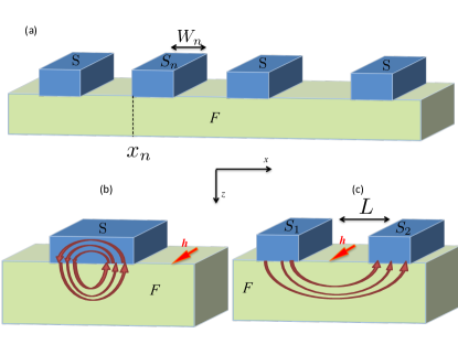
Figure 1: Lateral S/F structures and illustration of the supercurrent flow.

In the two-terminal case, shown on Fig. 1c, the total current $I_{1}$ flowing through S1-terminal is nonzero due to $f_{s}^{{\rm Re}}(x)$ induced from S2-terminal:

$$I_{1} = \frac{\pi k_{h}^{2}\theta T}{eR_{b1}R_{b2}\sigma_{0}}\sum_{\omega}f_{BCS}$$

$$\times \int_{x_{1}}^{x_{1}+W_{1}}dx\left[s(x-x_{2})-s(x-x_{2}-W_{2})\right]$$

Therefore besides currents circulating around each interface, there is a finite Josephson current induced by mutual effect of extrinsic SOC and the exchange field (see Fig. 1c). This supercurrent at $\varphi=0$ resembles the anomalous current in a $\varphi_{0}$-junction studied in the context of intrinsic SOC in polar crystals (Bergeret and Tokatly, 2015; Konschelle et al., 2015; Buzdin, 2008). Here we show that $\varphi_{0}$-junction can be built out of the most common inversion symmetric materials provided they show a finite exchange spin-splitting and a SH-angle. The anomalous current is proportional to $\theta h$, which in turn is proportional to the anomalous Hall conductivity $\sigma_{AH}$ in ferromagnets (Nagaosa et al., 2010). Hence F materials with large $\sigma_{AH}$ are good candidates for showing an anomalous supercurrent in lateral SFS structures. If for example one uses a ferromagnet with strong exchange field such that $k_{h}^{2}\gg k_{so}^{2}$, the amplitude of the anomalous current is according to our theory proportional to $\theta$ times the critical current of the junction.Thus, for materials with $\theta\sim 5-20\%$ the anomalous phase current can be detected by using quantum interferometer devices as done for example in Ref.delft for nanowires.

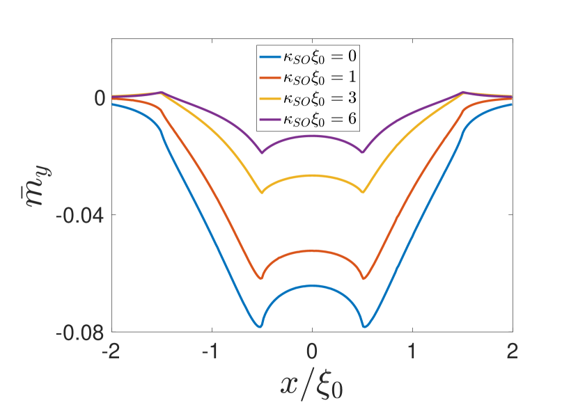
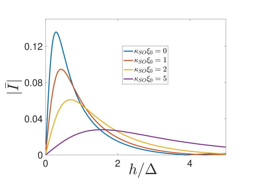
Figure 2: Left panel: the x-dependence of the induced magnetic moment $\bar{m}^{y}=m^{y}/(\pi\mu_{B}N_{0}\theta\gamma_{1}\gamma_{2}D)$ at $z=0$ for a symmetric lateral SNS junction with $L=1$, $W=1$ and $\varphi=\frac{\pi}{2}$. Right panel: induced anomalous supercurrent as a function of the exchange field for $L=1$ and W=5. We have chosen $T=0.1$. and defined $\xi_{0}=\sqrt{D/2\Delta}$.

In the right panel of Fig. 2 we show the anomalous current through the S1-terminal as a function of the field $h$. The current starts from zero at $h=0$, reaches a maximum and finally decays for large fields because of the usual suppression of superconductivity by the $h$ field (Buzdin, 2005; Bergeret et al., 2005). Inversely, if $h=0$ a finite Josepshon current ($\varphi\neq 0$) between the two S electrodes induces a finite magnetic moment (see SM for details) similar to the situation found in the S and S/N layered systems. In the left panel of Fig. 2 we show the $x$-dependence of the magnetic moment induced at $z=0$.

In conclusion, we have presented a new theoretical framework that describes diffusive superconducting hybrid structures with extrinsic SOC. We have derived equations that contain hitherto unknown terms proportional to the SH-angle, responsible in the normal state for the SHE, and the Lifshits-Dyakonov spin-currents swapping parameter. Our equations pave the way to explore numerous novel effects in the field of superconducting spintronics Wakamura ; Maekawa ; Reviews and open up numerous opportunities for the control of charge and spin currents in the non-dissipative regime. As illustrative examples we demonstrate the existence of magnetoelectric effects in different superconducting structures. We show that these effects are proportional to the SH-angle and hence can be observed by combining materials with known large $\theta$, like Pt or Co, with superconducting electrodes.

I Supplementary Material

I.1 Derivation of the Usadel equation in the presence of extrinsic spin-orbit coupling

In this section we derive the generalised Usadel equation to account for magnetoelectric effects [Eq. (5) in the main text]. We consider a diffusive conventional superconductor described by the Hamiltonian

$$H=H_{BCS}-{\bf h}{\bm{\sigma}}+\hat{W}(\mathbf{r})\;,$$ (13)

where $H_{BCS}$ is the usual mean field BCS Hamiltonian, ${\bf h}$ is the exchange field, ${\bm{\sigma}}=(\sigma_{1},\sigma_{2},\sigma_{3})$ the Pauli matrices, and $\hat{W}({\bf r})$ is a random impurity potential

$$\hat{W}({\bf r})=V({\bf r})+\hat{V}_{SOC}(\mathbf{r})\;.$$ (14)

It consists of the usual (scalar) elastic scattering $V({\bf r})$ and the spin-orbit part

$$\hat{V}_{SO}=\lambda^{2}\left({\bf\nabla}V(\mathbf{r})\times\hat{\mathbf{p}}\right){\bm{\sigma}}\;,$$ (15)

where the coupling constant is proportional to the effective Compton wavelength $\lambda$ squared and $\hat{{\bf p}}=-i\nabla_{{\bf r}}$ the momentum operator. In order to derive the quantum diffusion equation we introduce the Keldysh matrix Green functions (GF) which is the $8\times 8$ matrix

$$\check{G}=\left(\begin{array}[]{cc}G^{R}&G^{K}\\ 0&G^{A}\end{array}\right)\;,$$

consisting of the retarded, advanced and Keldysh 4$\times$4 matrices ($G^{R,A,K}$) in the Nambu-spin space. $\check{G}$ obeys the equationLangenberg and Larkin (1986)

$$\left[\tau_{3}i\partial_{t}+\frac{1}{2m}\partial_{r}^{2}+\mu+{\bf h}{\bm{\sigma}}+\check{\Delta}-\check{\Sigma}\right]\check{G}({\bf r},t;{\bf r^{\prime}},t^{\prime})=\delta({\bf r-r^{\prime}})\delta(t-t^{\prime})\;,$$ (16)

where $\mu$ is the chemical potential, $\check{\Delta}$ the superconducting order parameter and $\check{\Sigma}$ is the self-energy due to the impurity scattering, Eq. (14). We treat the latter within the self-consistency Born approximation, i.e.

$$\check{\Sigma}({\bf r_{1}},{\bf r_{2})}=\left\langle\hat{W}({\bf r_{1})\check{G}({\bf r_{1},{\bf r_{2})\hat{W}({\bf r}_{2})}}}\right\rangle=\check{\Sigma_{0}}+\check{\Sigma}_{1}+\check{\Sigma_{2}\;,}$$

where $\langle...\rangle$ denotes average over the impurity configuration. The three terms on the r.h.s correspond to the following contributions:

The usual elastic scattering term

$$\Sigma_{0}=\left\langle V({\bf r_{1}})\check{G}({\bf r_{1}},{\bf r_{2}})V({\bf r_{2}})\right\rangle\;,$$ (17)

the spin relaxation term which, quadratic in the SOC potential

$$\Sigma_{2}=\left\langle\hat{V}_{SO}({\bf r_{1}})\check{G}({\bf r_{1}},{\bf r_{2}})\hat{V}_{SO}({\bf r_{2}})\right\rangle$$ (18)

and the “mixed” term

$$\Sigma_{1}=\left\langle V({\bf r_{1}})\check{G}({\bf r_{1}},{\bf r_{2}})\hat{V}_{SO}({\bf r_{2}})\right\rangle+\left\langle\hat{V}_{SO}({\bf r_{1}})\check{G}({\bf r_{1}},{\bf r_{2}})V({\bf r_{2}})\right\rangle$$ (19)

which is responsible for the coupling between charge and spin degrees of freedom and leads to the SHE and AHE. As usual, we assume for the random potential

$$\langle V({\bf r_{1}})V({\bf r_{2}})\rangle=\frac{1}{2\pi N_{F}\tau}\delta({\bf r_{1}}-{\bf r_{2}})\;,$$ (20)

where $\tau$ is the momentum relaxation time.

We follow the usual steps in order to obtain the quantum kinetic equation from Eq. (16)Langenberg and Larkin (1986): (1) One subtracts from Eq. (16) its conjugate, (2) performs the Wigner transform and then (3) the gradient expansion. After these steps are carried out one obtains the kinetic-like equation [Eq. (1) in the main text]:

$$\frac{p_{k}}{m}\partial_{k}G+i\tau_{3}\partial_{t}G-i\partial_{t^{\prime}}G\tau_{3}+i\left[\mathbf{h}{\bm{\sigma}}\tau_{3},G\right]={\cal I}\;,$$ (21)

where ${\cal I}=-i\left[\check{\Sigma},\check{G}\right]={\cal I}_{0}+{\cal I}_{1}+{\cal I}_{2}$ is the collision term. It consists of three contributions corresponding to the three self-energy terms (17-19). ${\cal I}_{0}$ and ${\cal I}_{2}$ can be treated in the lowest order of the gradient expansion. In contrast and in order to catch consistently the charge-spin coupling we need to include linear terms of ${\cal I}_{1}$ in the gradient expansion:

$${\cal I}_{1}({\bf r},{\bf p})=-i\left[\check{\Sigma}_{1{\bf p}},\check{G}_{{\bf p}}\right]+\frac{1}{2}\left\{\partial_{{\bf r}}\check{\Sigma}_{1{\bf p}},\partial_{{\bf p}}\check{G}_{{\bf p}}\right\}-\frac{1}{2}\left\{\partial_{{\bf p}}\check{\Sigma}_{1{\bf p}},\partial_{{\bf r}}\check{G}_{{\bf p}}\right\}\dots\;.$$ (22)

The derivation of the quasiclassical expressions for ${\cal I}_{0,2}$ follows the standard steps, and hence those terms will be added straightforwardly in the end equation. Here we focus on the term ${\cal I}_{1}$ and how to include it in the quasiclassical formalism.

We start by writing explicitly the self-energy Eq. (19):

$$\Sigma_{1}=-i\langle A_{j}^{a}({\bf r_{1}})V({\bf r_{2}})\rangle\partial_{{\bf r}_{1}^{j}}\sigma^{a}G({\bf r_{1}},{\bf r_{2}})+i\langle A_{j}^{a}({\bf r_{2}})V({\bf r_{1}})\rangle\partial_{{\bf r}_{2}^{j}}G({\bf r_{1}},{\bf r_{2}})\sigma^{a}\;,$$ (23)

where

$$A_{j}^{a}({\bf r_{1}})=\lambda^{2}\epsilon_{kja}\partial_{{r_{1}^{k}}}V({\bf r_{1}})\;,$$

$\epsilon_{ijk}$ is the Levi-Civita tensor, and sum over repeated indices is implied.

By using Eq. (20) one obtains:

$$\Sigma_{1}=-i\frac{\lambda^{2}}{2\pi N_{F}\tau}\epsilon_{kja}\partial_{{\bf r}_{1}^{k}}\delta({\bf r_{1}-r_{2}})\sigma^{a}\partial_{{\bf r}_{1}^{j}}G({\bf r_{1},r_{2}})+i\frac{\lambda^{2}\epsilon_{kja}}{2\pi N_{F}\tau}\partial_{{\bf r}_{2}^{k}}\delta({\bf r_{1}-r_{2}})\partial_{{\bf r}_{2}^{j}}G({\bf r_{1},r_{2}})\sigma^{a}\;.$$

Now we Wigner-transform this expression. This implies to go over the relative ${\bm{\rho}}{\bf={\bf r_{1}-r_{2}}}$ and center of mass coordinates ${\bf r}={\bf(r_{1}}+{\bf r_{2}})/2$ and to Fourier- transform with respect to ${\bm{\rho}}$:

$$\Sigma_{1}({\bf r},{\bm{p}})=-i\frac{\lambda^{2}\epsilon_{kja}}{2\pi N_{F}\tau}\sum_{\bm{p^{\prime}}}\int{\bm{d\rho}}e^{-i{\bm{\rho}}({\bm{p}}-{\bm{p^{\prime}}})}\partial_{\rho^{k}}\delta({\bm{\rho}})\left(ip^{\prime}_{j}\left[\sigma^{a},G(\bm{p^{\prime}})\right]+\frac{1}{2}\partial_{r^{j}}\left\{\sigma^{a},G(\bm{p^{\prime}})\right\}\right)\;.$$ (24)

By noticing that $\sum_{\bm{p}}\epsilon_{ija}p_{i}p_{j}G^{a}(\bm{p})=0$ and that the Green’s functions are peaked at the Fermi level we can express $\Sigma_{1}$ in terms of the quasiclassical GFs $g=(i/\pi)\int d\xi G$ as:

$$\Sigma_{1}=\frac{\lambda^{2}\epsilon_{kja}}{2\tau}\left[\sigma^{a},p_{k}\langle p_{j}g\rangle\right]-i\frac{\lambda_{c}^{2}\epsilon_{kja}}{2\tau}\partial_{r^{j}}\left\{\sigma^{a},p_{k}\langle g\rangle-\langle p_{k}g\rangle\right\}\;.$$ (25)

In this last expression the brackets denote average over the momentum direction. It is important to note that the second term contains a gradient and hence it is, in principle, of smaller order than the first one in the gradient expansion. As noticed before, the description of the spin-charge coupling compels to keep these higher order terms.

We substitute now Eq. (25) into the expression for the collision term Eq. (22) and keep terms up to linear order in the gradients:

$${\cal I}_{1}\approx-i\left[\Sigma_{1}^{(0)},G_{\bm{p}}\right]-i\left[\Sigma_{1}^{(1)},G_{\bm{p}}\right]+\frac{1}{2}\left\{\partial_{{\bf r}}\Sigma_{1{\bf p}}^{(0)},\partial_{{\bf p}}G_{{\bf p}}\right\}-\frac{1}{2}\left\{\partial_{{\bf p}}\check{\Sigma}_{1{\bf p}}^{(0)},\partial_{{\bf r}}\check{G}_{{\bf p}}\right\}\;,$$ (26)

where $\Sigma_{1\bm{p}}^{(0,1)}$ are the first and second term in Eq. (25) respectively. We emphasise once again that in order to get the next-leading order correction correctly it is crucial to keep all terms in the expansion Eq. (22).

The collision term described by Eq. (26) does not allow for a straightforward integration over the quasiparticle energy and hence one cannot derive a closed differential equation (Eilenberger equation) for the quasiclassical $\check{g}$. In order to overcome this difficulty we consider the diffusive limit and derive equations for the zeroth $\sum_{{\bf p}}\check{G}$ and first $\sum_{{\bf p}}{\bf p}\check{G}$ moments of $\check{G}$.

From Eq. (26) we obtain :

$$\frac{i}{\pi N_{F}}\sum_{\bm{p}}{\cal I}_{1}=\epsilon_{kja}\frac{\lambda^{2}}{4\tau}\left(i\left\{\sigma^{a},\left[\langle p_{k}g\rangle,\langle p_{j}g\rangle\right]\right\}+\partial_{k}\left\{\sigma^{a},\left[\langle g\rangle,\langle p_{j}g\rangle\right]\right\}-\left[\sigma^{a},\left\{\langle g\rangle,\partial_{k}\langle p_{j}g\rangle\right\}\right]\right)\;,$$ (27)

for the zeroth moment of ${\cal I}_{1}$ and

$$\frac{i}{\pi N_{F}}\sum_{\bm{p}}p_{k}{\cal I}_{1}=-\epsilon_{kja}\frac{\lambda^{2}p_{F}^{2}}{2\tau}\frac{1}{3}\left(i\left[\left[\sigma^{a},\langle p_{j}g\rangle\right],\langle g\rangle\right]+\frac{1}{2}\left[\left\{\sigma^{a},\partial_{j}\langle g\rangle\right\},\langle g\rangle\right]\right)$$ (28)

for the first moment.

In the diffusive limit one assumes that $\tau E\ll 1$ and $\lambda^{2}p_{F}^{2}\ll 1$( $E$ is any energy involved in the kinetic equation) and expands $g$ in spherical harmonics: $g\approx g_{0}+n_{k}g_{k}$ such that $\langle g\rangle=g_{0}$, $\langle p_{k}g\rangle=p_{F}g_{k}$, and $g_{0}\gg g_{k}$, . In this limit one can simplify expressions (27-28) and get:

$$\frac{i}{\pi N_{F}}\sum_{\bm{p}}{\cal I}_{1}\approx\epsilon_{kja}\frac{\lambda^{2}p_{F}}{4\tau}\left(\partial_{k}\left\{\sigma^{a},\left[g_{0},g_{j}\right]\right\}-\left[\sigma^{a},\left\{g_{0},\partial_{k}g_{j}\right\}\right]\right)$$ (29)

and

$$\frac{i}{\pi N_{F}}\sum_{\bm{p}}p_{k}{\cal I}_{1}\approx-\epsilon_{kja}\frac{\lambda^{2}p_{F}^{2}}{4\tau}\frac{1}{3}\left(i\left[\left[\sigma^{a},g_{j}\right],g_{0}\right]+\frac{1}{2}\left[\left\{\sigma^{a},\partial_{j}g_{0}\right\},g_{0}\right]\right)\;.$$ (30)

By switching to the Matsubara representation in Eq. (16) we obtain for the zero and first moments

$$\partial_{k}\left(v_{F}g_{k}-\epsilon_{kja}\frac{\lambda^{2}p_{F}}{4\tau}\left\{\sigma^{a},\left[g_{0},g_{j}\right]\right\}\right)+\left[(\omega-i{\bf h}{\bm{\sigma})\tau_{3},}g_{0}\right]=-\frac{1}{8\tau_{SO}}\left[\sigma^{a}g_{0}\sigma^{a},g_{0}\right]-\epsilon_{kja}\frac{\lambda^{2}p_{F}}{4\tau}\left[\sigma^{a},\left\{g_{0},\partial_{k}g_{j}\right\}\right]$$ (31)

and

$$\frac{\tau v_{F}}{3}\partial_{k}g_{0}+\epsilon_{kja}\frac{\lambda^{2}p_{F}}{4}\frac{1}{3}\left[\left\{\sigma^{a},\partial_{j}g_{0}\right\},g_{0}\right]=-\frac{1}{2}\left[g_{0},g_{k}\right]+\epsilon_{kja}\frac{\lambda^{2}p_{F}^{2}}{2}\frac{i}{3}\left[\left[\sigma^{a},g_{j}\right],g_{0}\right]\,,$$ (32)

where $1/\tau_{SO}=8\lambda^{4}p_{F}^{4}/9\tau$, and in the second equation we only took leading order terms in the diffusive expansion. At this stage and before writing the Usadel equation, it is worth to make two remarks: (i) The first term in Eq. (31) is the divergence of the matrix current

$$\check{J}_{k}=v_{F}g_{k}-\epsilon_{kja}\frac{\lambda^{2}p_{F}}{4\tau}\left\{\sigma^{a},\left[g_{0},g_{j}\right]\right\}\;.$$ (33)

The last term of this expression stems form the SOC and described the coupling between the charge and spin currents. (ii) The structure of Eq. (32), $\partial_{k}g_{0}+[A,g_{0}]=0$, ensures the validity of the normalization condition

$$g_{0}^{2}=1\;.$$ (34)

The final step is to get an expression for the anisotropic component $g_{k}$ in terms of the isotropic one $g_{0}$ from Eq. (32). In leading order with respect to the parameters $\lambda^{2}p_{F}^{2}$ and $\lambda^{2}p_{F}/L$, where $L$ is the characteristic length over which $g_{0}$ varies, the anisotropic component reads

$$g_{k}=-\tau v_{F}g_{0}\partial_{k}g_{0}+\epsilon_{kja}\frac{\lambda^{2}p_{F}}{2}\left\{\sigma^{a},\partial_{j}g_{0}\right\}-\epsilon_{kja}\lambda^{2}p_{F}^{2}\frac{i}{3}\left[\sigma^{a},\tau v_{F}g_{0}\partial_{j}g_{0}\right]\;.$$ (35)

This can be checked by substituting Eq. (35) into Eq. (32), using the normalization condition (34), and by keeping only leading order terms. If we now substitute this expression for $g_{k}$ into Eq. (33) we obtain the expression of the matrix current in terms of $g_{0}$:

$$J_{k}=-D\left(g_{0}\partial_{k}g_{0}-\frac{\theta}{2}\epsilon_{kja}\left\{\sigma^{a},\partial_{j}g_{0}\right\}+i\frac{\kappa_{sw}}{2}\epsilon_{kja}\left[\sigma^{a},g_{0}\partial_{j}g_{0}\right]\right)\;.$$ (36)

Here $\theta$ is the spin-Hall angle defined as $\theta=2\lambda^{2}p_{F}/v_{f}\tau=l_{s0}/l$ and $\kappa_{sw}$ the “swapping” term $\kappa_{sw}=2\lambda^{2}p_{F}^{2}/3$Lifshits and Dyakonov (2009).

Finally, by substituting Eq. (LABEL:gani) into Eq. (31) we obtain the Usadel equation:

$$\partial_{k}J_{k}+\left[(\omega-i{\bf h}\mathbf{\sigma)\tau_{3},}g_{0}\right]=-\frac{1}{8\tau_{SO}}\left[\sigma^{a}g_{0}\sigma^{a},g_{0}\right]+\epsilon_{kja}\frac{\lambda_{c}^{2}p_{F}}{4}v_{F}\left[\sigma^{a},\left\{g_{0},\frac{1}{3}\partial_{k}g_{0}\partial_{j}g_{0}\right\}\right]\;.$$ (37)

Terms with two derivatives acting on the same $g$, i.e. $\partial_{k}\partial_{j}g$ after summation over indices vanish because of the antisymmetric tensor $\epsilon_{ijk}$. By substitution of Eq. (36) into Eq. (37) and going back to the real times representation one obtains Eq. (5) of the main text.

The generalisation of the Kupriyanov-Lukichev boundary condition at hybrid interfaces is straightforward from the current expression Eq. (36) (we omit here the index $0$ in $G_{0}$):

$$\check{g}\partial_{k}\check{g}-\theta_{SH}\epsilon_{kja}\left\{\sigma^{a},\partial_{j}\check{g}\right\}+i\kappa_{sw}\epsilon_{kja}\left[\sigma^{a},\check{g}\partial_{j}\check{g}\right]=-\frac{1}{2R_{b}\sigma_{F}}\left[g_{BCS},\hat{g}\right]\;,$$ (38)

Observables like the charge current and magnetic moment can be expressed in terms of the quasiclassicla Green’s functions:

$$j_{k}=\frac{i\pi T}{16e}\sigma_{F}\sum_{\omega}{\rm Tr}\tau_{3}\check{J_{k}}$$ (39)

and

$$m^{a}=\frac{\mu_{B}i\pi N_{0}T}{4}\sum_{\omega}Tr\tau_{3}\sigma^{a}\check{g}\;.$$ (40)

We should notice that in the normal case Eq. (37) simplifies drastically: First the retarded and advanced GFs equals to $\pm 1$ respectevely and hence there is only on equation for the Keldysh component which in such a case consist on the charge and spin distribution functions $g^{K}=f_{c}+f_{s}^{a}\sigma^{a}$. Second the equation can be straightfoirwarly integrated over energies and hence instead of writing the equations for $f_{c}$, $f_{s}^{a}$ one write them for the charge and the spin density $n\sim\int dEf_{c}(E)$ and $S^{a}\sim\int dEf_{s}^{a}(E)$. In particular by simple

I.2 Solution of the Usadel equation for a lateral multi-terminal S-F structure

Let us consider the geometry shown if Fig. 1 of the main text and calculate the current through the $n$-th S/F interface, which is given by Eq. (11) in the main text. Thus, we need to determine the real part of the singlet component of the condensate induced in N. In the geometry under consideration with an exchange field in $y$ direction, the anomalous GFs $\hat{f}=f_{s}+{\rm sgn}(\omega)\sigma^{y}f_{t}$ depends on two coordinates $x$ and $z$. It is convenient to introduce the Fourier component $\hat{f}(q,z)$ with respect to $x$,

$$\hat{f}(x,z)=\int dqe^{iqx}\hat{f}(q,z)$$

The singlet and triplet components then satisfy the following equations,

$$\partial_{zz}^{2}f_{s}(q,z)-(k_{\omega}^{2}+q^{2})f_{s}(q,z)-ik_{h}^{2}f_{t}(q,z) = 0$$ (41)

$$\partial_{zz}^{2}f_{t}(q,z)-(k_{\omega}^{2}+q^{2}+k_{so}^{2})f_{t}(q,z)-ik_{h}^{2}f_{t}(q,z) = 0$$ (42)

with boundary conditions at $z=0$

$$\partial_{z}f_{s}(q,0)-iq\theta f_{t}(q,0) = if_{BCS}F_{0}(q)$$ (43)

$$\partial_{z}f_{t}(q,0)-iq\theta f_{s}(q,0) = 0\quad,$$ (44)

where $F_{0}(q)$ is the Fourier transform of the r.h.s of the boundary condition at the S-electrodes described by

$$F_{0}(x)=\sum\gamma_{n}e^{i\varphi_{n}}\left[\Theta(x-x_{n})-\Theta(x-x_{n}-W_{n})\right]\quad,$$

and $\gamma_{n}=1/R_{bn}\sigma_{0}$. Let us assume that $\varphi_{n}=0$ for all S terminals. According to Eq. (11) in the main text, to obtain the current through the nth S/N boundary we only need to calculate the real part of the singlet component, $f_{s}^{Re}(x)={\rm Re}f_{s}(x,0)$ at the S/F interface ($z=0$). One can straightforwardly verify from Eqs. (41)-(44) that in the linear order in $\theta$ the Fourier component $f_{s}^{Re}(q)$ of $f_{s}^{Re}(x)$ is given by

$$f_{s}^{Re}(q)=ik_{h}^{2}\theta qF_{0}(q)s(q)\;,$$

where

$$\frac{s(q)}{f_{BCS}}=\frac{1}{(k_{+}^{2}-k_{-}^{2})^{2}}\left[\frac{k_{-}^{2}-k_{\text{$\omega$}}^{2}}{2\left(q^{2}+k_{+}^{2}\right)}+\frac{k_{+}^{2}-k_{\text{$\omega$}}^{2}}{2\left(q^{2}+k_{-}^{2}\right)}-\frac{2k_{SO}^{2}}{\sqrt{q^{2}+k_{+}^{2}}\sqrt{q^{2}+k_{-}^{2}}}\right]\;,$$ (45)

and $k_{\pm}^{2}=k_{\omega}^{2}+k_{so}^{2}/2\pm\sqrt{(k_{so}^{2}/2)^{2}-k_{h}^{4}}$. Thus, $f_{s}^{Re}(x)$ can be obtained by transforming back

$$f_{s}^{Re}(x)=k_{h}^{2}\theta\int dx_{1}\left[\partial_{x_{1}}F_{0}(x_{1})\right]s(x-x_{1})$$ (46)

Since $F_{0}$ is a combination of step functions its spatial derivative gives a sum of delta-functions, thus:

$$f_{s}^{Re}(x)=k_{h}^{2}\theta\sum_{n}\gamma_{n}\left[s(x-x_{n})-s(x-x_{n}-W_{n})\right]\;.$$ (47)

The inverse Fourier transform of the function $s(q)$, Eq. (45) can be written explicitly as

$$\frac{s(x)}{f_{BCS}}=\frac{k_{-}^{2}-k_{\omega}^{2}}{k_{+}(k_{+}^{2}-k_{-}^{2})^{2}}e^{-k_{+}|x|}+\frac{k_{+}^{2}-k_{\omega}^{2}}{k_{-}(k_{+}^{2}-k_{-}^{2})^{2}}e^{-k_{-}|x|}-\frac{2k_{so}^{2}}{\pi^{2}(k_{+}^{2}-k_{-}^{2})^{2}}\int dx_{1}K_{0}(k_{+}|x_{1}|)K_{0}(k_{-}|x-x_{1}|)\;,$$ (48)

where $K_{0}$ is the modified Bessel function of second kind. Expressions (47-48) have been used to compute the current from Eq. (11) in the main text.

Now we consider a symmetric lateral structure with two S electrodes (see Fig. 1c) of width $W$ at a distance $L$ from each other. We assume that $h=0$ and a finite phase difference $\varphi$ between the superconductors. According to Eqs. (41-44) the solutions for the singlet and triplet components are

$$f_{s}(q,z) = -\frac{if_{BCS}}{\kappa_{s}}F_{0}(q)e^{-k_{s}z}$$ (49)

$$f_{t}(q,z) = -\frac{q\theta f_{BCS}}{k_{s}k_{t}}F_{0}(q)e^{-k_{t}z}$$ (50)

where $k_{s}^{2}=k_{\omega}^{2}+q^{2}$and $k_{t}^{2}=k_{\omega}^{2}+k_{so}^{2}+q^{2}$ and $F_{0}(q)$ is the Fourier transform

$$F_{0}(x)=\gamma_{1}e^{-i\varphi/2}\left[\Theta(x+L/2+W)-\Theta(x+L/2)\right]+\gamma_{2}e^{i\varphi/2}\left[\Theta(x-L/2)-\Theta(x-L/2-W)\right]$$

We calculate here the magnetic moment at $z=0$ that is given by

$$m^{y}=2\pi\mu_{B}N_{0}T\sum_{\omega}{\rm Im}f_{s}^{*}(x,0)f_{t}(x,0)$$ (51)

We need then to determine the Fourier transform of the prefactors in Eq. (4950). In particular

$$f_{s}(x,0)=-if_{BCS}\int dx^{\prime}F_{0}(x^{\prime})\frac{1}{\pi}K_{0}(k_{\omega}|x-x^{\prime}|)$$

and

$$f_{t}(x,0)=i\theta f_{BCS}\int dx^{\prime}\partial_{x^{\prime}}F_{0}(x^{\prime}){\cal F}(x-x^{\prime})\;,$$

with

$${\cal F}(x-x^{\prime})=\int\frac{dx^{\prime\prime}}{\pi^{2}}K_{0}(\sqrt{k_{\omega}^{2}+k_{so}^{2}}|x^{\prime\prime}|)K_{0}(k_{\omega}|x-x^{\prime}-x^{\prime\prime}|)$$

Substitution of these expressions into Eq.51 gives

$$m^{y}(x)=2\pi\gamma_{L}\gamma_{R}\mu_{B}N_{0}T\theta\sin\varphi\sum_{n} \left\{\int_{L/2}^{L/2+W}dx^{\prime}K_{0}\left(k_{\omega}|x-x^{\prime}|\right)\left[{\cal F}(x+\frac{L}{2}+W)-{\cal F}(x+\frac{L}{2})\right]\right. -$$

$$-\left.\int dx^{\prime}K_{0}\left(k_{\omega}|x-x^{\prime}|\right)\left[{\cal F}(x-\frac{L}{2})-{\cal F}(x-\frac{L}{2}-W)\right]\right\}$$

This is the function plotted in the left panel of Fig. 2.

References

• Sinova et al. (2015) J. Sinova, S. O. Valenzuela, J. Wunderlich, C. Back,  and T. Jungwirth, Reviews of Modern Physics 87, 1213 (2015).
• Nagaosa et al. (2010) N. Nagaosa, J. Sinova, S. Onoda, A. MacDonald,  and N. Ong, Reviews of Modern Physics 82, 1539 (2010).
• Zutic et al. (2004) I. Zutic, J. Fabian,  and S. Das Sarma, Reviews of Modern Physics 76, 323 (2004).
• Edelstein (1995) V. M. Edelstein, Physical Review Letters 75, 2004 (1995).
• Bergeret and Tokatly (2015) F. S. Bergeret and I. V. Tokatly, Europhysics Letters (EPL) 110, 57005 (2015)arXiv:1409.4563 .
• Konschelle et al. (2015) F. Konschelle, I. V. Tokatly,  and F. S. Bergeret, Physical Review B 92, 125443 (2015)arXiv:1506.02977 .
• Mal’shukov and Chu (2008) A. Mal’shukov and C. Chu, Physical Review B 78, 104503 (2008)arXiv:0801.4419 .
• Mal’shukov et al. (2010) A. G. Mal’shukov, S. Sadjina,  and A. Brataas, Physical Review B 81, 060502 (2010).
• Abrikosov and Gorkov (1962) A. Abrikosov and L. Gorkov, Sov. Phys. JETP 15, 752 (1962).
• Demler et al. (1997) E. A. Demler, G. B. Arnold,  and M. R. Beasley, Physical Review B 55, 15174 (1997).
• Bergeret et al. (2005) F. S. Bergeret, A. F. Volkov,  and K. B. Efetov, Reviews of Modern Physics 77, 1321 (2005).
• Bergeret and Tokatly (2014) F. S. Bergeret and I. V. Tokatly, Physical Review B 89, 134517 (2014)arXiv:1402.1025 .
• (13) For details see supplementary material.
• Langenberg and Larkin (1986) D. N. Langenberg and A. I. Larkin, Nonequilibrium superconductivity (North-Holland, Amsterdam, 1986).
• Alexander et al. (1985) J. Alexander, T. Orlando, D. Rainer,  and P. Tedrow, Physical Review B 31, 5811 (1985).
• Volkov et al. (2007) A. F. Volkov, F. S. Bergeret,  and K. B. Efetov, Physical Review B 75, 184510 (2007).
• Raimondi and Schwab (2010) R. Raimondi and P. Schwab, Physica E: Low-dimensional Systems and Nanostructures 42, 952 (2010).
• Shen et al. (2014) K. Shen, R. Raimondi,  and G. Vignale, Phys. Rev. B 90, 245302 (2014).
• Lifshits and Dyakonov (2009) M. B. Lifshits and M. I. Dyakonov, Physical Review Letters 103, 186601 (2009).
• Kupriyanov and Lukichev (1988) M. Y. Kupriyanov and V. F. Lukichev, Sov. Phys. JETP 67, 1163 (1988).
• Buzdin (2008) A. I. Buzdin, Physical Review Letters 101, 107005 (2008)arXiv:0808.0299 .
• Buzdin (2005) A. I. Buzdin, Reviews of Modern Physics 77, 935 (2005).
• (23) R S Keizer, S T B Goennenwein, T. M. Klapwijk, G Miao, G Xiao, and A Gupta, Nature, 439 (2006).
• (24) M. Anwar, F. Czeschka, M. Hesselberth, M. Porcu, and J. Aarts, Physical Review B, 82 (2010).
• (25) Jian Wang, Meenakshi Singh, Mingliang Tian, Nitesh Kumar, Bangzhi Liu, Chuntai Shi, J. K. Jain, Nitin Samarth, T. E. Mallouk, and M. H. W. Chan, Nature Physics, 6 389 (2010).
• (26) A. Singh, S. Voltan, K. Lahabi, and J. Aarts, Phys. Rev. X, 5 (2015).
• (27) T. Wakamura, N. Hasegawa, K. Ohnishi, Y. Niimi, and Y. Otani, Phys. Rev. Lett. 112, 036602 (2014).
• (28) S. Takahashi and S. Maekawa, Japanese Journal of Applied Physics 51, 010110 (2011).
• (29) M. Eschrig Phys. Today 64, 43 (2011); J. Linder and J. W. A. Robinson, Nature Physics 11, 307 (2015).
• (30) D. B. Szombati, S. Nadj-Perge, D. Car, S. R. Plissard, E. P. A. M. Bakkers and L. P. Kouwenhoven, Nat. Phys. 12, 568?572 (2016).