Nonlinear waves in the terrestrial quasi-parallel foreshock
Abstract
We study the applicability of the derivative nonlinear Schrödinger (DNLS) equation, for the evolution of high frequency nonlinear waves, observed at the foreshock region of the terrestrial quasi-parallel bow shock. The use of a pseudo-potential is elucidated and, in particular, the importance of canonical representation in the correct interpretation of solutions in this formulation is discussed. Numerical solutions of the DNLS equation are then compared directly with the wave forms observed by Cluster spacecraft. Non harmonic slow variations are filtered out by applying the empirical mode decomposition. We find large amplitude nonlinear wave trains at frequencies above the proton cyclotron frequency, followed in time by nearly harmonic low amplitude fluctuations. The approximate phase speed of these nonlinear waves, indicated by the parameters of numerical solutions, is of the order of the local Alfvén speed.
pacs:
Valid PACS appear hereIntroduction. Magnetised plasmas constitute a dielectric medium in which finite amplitude fluctuations experience nonlinear evolution and interactions. This can lead to wave steepening Cohen74 , self-focusing Zakharov ; Hasegawa and to parametric instabilities, which may proceed towards fully developed turbulence Robinson . Understanding the nonlinear evolution of large amplitude Alfvén and the fast magnetosonic waves, their transition to quasi-parallel turbulence as well as their coexistence with the oblique strong turbulence, is fundamental to the physics of astrophysical collisionless shocks Kennel88 and solar wind turbulence Belcher ; Sharma15 . Large amplitude magnetic field fluctuations have been directly observed in the terrestrial Eastwood03 and interplanetary Kajdic12 foreshocks, but are also important for supernova shocks and the acceleration of galactic cosmic rays Bell78 . The parallel wave vector component of solar wind turbulence is poorly understood and its clear detection remains elusive He11 .
Various nonlinear equations have been constructed for magnetohydrodynamic (MHD) waves in the past. In a weakly dispersive medium, nonlinear propagating waves evolve according to the Korteweg-de Vries (KdV) equation and historically, this model attracted most studies. For example, finite amplitude slow and fast MHD waves propagating across, or at large oblique angles with respect to the magnetic field, were shown to obey the KdV equation Kukutani69 . For MHD fluctuations propagating parallel, or nearly parallel, to the background equilibrium magnetic field, the derivative nonlinear Schrödinger equation (DNLS) proved to be a good description Rogister71 ; Cohen74 ; Mjolhus89 ; Kennel88 . The DNLS equation has been studied analytically Hada for homogeneous media and numerically for the inhomogeneous case, e.g Buti . A range of numerical studies was also performed for the cases with dissipation Ghosh and heat flux Medvedev . Beyond MHD approximations, high-frequency nonlinear fluctuating structures on the whistler dispersion branch, exhibiting soliton-like features, have been identified in numerical and analytical studies, e. g. Sauer02 ; Dubinin03 .
Upstream regions of quasi-parallel astrophysical shocks are among the most complex plasma systems. The lack of collisions requires multi-scale collective dynamics to mediate energy dissipation and isotropy in these regions. The terrestrial foreshock offers an opportunity to validate predictions of theoretical shock models against in situ spacecraft observations Burgess97 ; Selzer14 . The presence of nonlinear waves in quasi-parallel foreshocks has important implications. Wave collapse and self-focusing generate strong electrostatic fields on kinetic scales, which accelerate particles, modifying their velocity distribution function Bale98 ; Graham15 . Increased viscous and Ohmic dissipation may occur in these regions dominated by strong gradients and shocks. In a warm plasma and for oblique-propagating waves, the magnetic field fluctuations interact with density and velocity perturbations and therefore affect the wave propagation speed as well as the wave evolution. Nonlinear interactions among the waves generate low frequency harmonics (condensate) and these may in turn become unstable to modulation instability.
We examine the foreshock region of the quasi-parallel terrestrial bow shock and, for the first time, quantify propagation characteristics and spatial structure of nonlinear high frequency waves by direct comparison of experimental observations and numerical solutions. First, we discuss the importance of canonical representation of the first integral of the DNLS in the correct interpretation of the solutions, based on a functional form of the pseudo-potential. In contrast with previous presentation Hada we obtain a pseudo-potential which diverges to infinity when its argument approaches zero or infinity, a behaviour which guarantees the existence of large amplitude oscillatory solutions. We then examine observations from the Cluster spacecraft and perform direct comparison of the nonlinear wave forms found in observations and these obtained from the numerical solutions of the DNLS.
Exact solutions of the DNLS. Consider a magnetised plasma with elliptically polarised Alfvén waves propagating in the quasi-parallel z-direction with the transverse components, . We define two characteristic speeds: sound speed, and the Alfvén speed , where is the adiabatic index, is the temperature, is the proton number density and is the proton mass. The evolution of these left and right-hand polarised modes, is described by the DNLS equation Hada :
| (1) |
In (1) the temporal and spatial variables have been normalised by the ion gyro-frequency, , and the ion inertial length , respectively. The constant , and corresponds to left (-) and right-hand (+) polarised mode. Writing the transverse components as , equation (1) separates into two equations for the fluctuating field amplitude, and its phase :
| (2) |
| (3) |
Following Hada , the phase angle is assumed to separate into its functional dependence such that , where is a constant and is an a priori unknown function of . In the frame of reference travelling with the phase velocity of the perturbation, (normalised by the Alfvén speed), that is taking , which eliminates temporal variations, one finds the first integral of (3) to be , where and is a constant.
Equation (2), expressed in the new variable , takes the following form:
| (4) |
where and . The first integral of (4) can then be found using Bernoulli’s method, which gives:
| (5) |
where
| (6) |
and is a new constant of integration. Treating and as a generalised coordinate and time of a pseudo-particle, the first and second terms on the left hand side of (5) represent generalised kinetic and potential energies written in the canonical form, and the constant of integration can be interpreted as the total energy of a particle, which depends only on the initial conditions. This subtle point is important because it is only the canonical functional form of the potential that can be used to predict the type of solutions of (1) Dubinov . If (5) is multiplied by , as was done in Hada , it is no longer in the canonical form. The new potential loses its dependence, and the constant of motion loses its traditional meaning. The new potential suggests that there is a finite initial energy for which solutions of (1) are no longer oscillatory, since appears to have a finite value when . The coefficients which describe the behaviour of when are in this case no longer related only to the initial condition. In contrast, the form of clearly shows that when and when , so the solutions of (1) are oscillatory for the arbitrarily large amplitudes. In order to compare the oscillatory solutions of (1) with the nonlinear wave forms found in the terrestrial foreshock we will solve (4) numerically, for different initial conditions and using experimentally measured plasma parameters.
Experimental Data and Methodology. The dataset corresponds to a foreshock crossing on at :-:UT. We examine three sub-intervals, hereafter referred to as I1, I2 and I3, each a few tens of seconds long. This foreshock crossing has been studied before in the context of wave characteristics and temperature anisotropy Narita03 ; Selzer14 . We use magnetic field measurement of samples per second from Cluster FGM instrument Balogh and second averaged measurements of plasma parameters from the CIS-HIA instrument Reme01 . The transverse magnetic field fluctuations, described by (1), are obtained using minimum variance coordinates, which is equivalent to solving an eigen-value problem for the measured magnetic field variance matrix Sonnerup98 .
Magnitude of the transverse magnetic field observations is processed using the Hilbert-Huang transform (HHT) spectral technique Huang98 , which is suitable for analysing non-stationary and non-harmonic fluctuations. Unlike traditional spectral methods based on the Fourier decomposition and wavelets, which are restricted by an a priori assignment of harmonic basis functions, the HHT technique uses the empirical mode decomposition (EMD), which expands the given signal onto a basis derived directly from the data. The stability of intrinsic modes detected with the EMD is evaluated using the noise–assisted ensemble empirical mode decomposition (EEMD) Wu09 . We note that we do not examine each empirical mode separately, but rather use this technique as a filter allowing us to find a non-harmonic trend in the signal, which can then be subtracted. This filtered signal is used to produce phase space portraits, which are compared directly to the ones obtained by numerical integration of the second order equation (4).
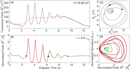
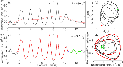
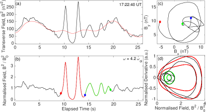
Results and Discussion. Figures 1-3 show nonlinear large amplitude quasi-parallel transverse waves for intervals I1, I2 and I3, respectively. Panel (a) of each figure shows the squared magnitude of the original transverse fluctuations, , in black and a non-harmonic trend, , determined with the EEMD technique, in red. We subtract this trend from the original signal and normalise the residue by the mean value of the first and the last point of the trend. This new signal, , where is the number of points in the signal, is plotted in panel (b) of each figure. We determine the frequency in the spacecraft frame, in units of , for the nonlinear (red) signal and these are given in the top right-hand corner of each panel (b). Colour dots mark the start of the nonlinear waves (red), end of nonlinear waves and transition to nearly harmonic fluctuations (blue) and the end of nearly harmonic fluctuations (green). Panels (c) show hodograms of the minimum variance transverse components of the magnetic field, which are left-hand polarised for all intervals, in the spacecraft frame of reference. Previous studies found modes propagating predominantly away from the bow shock for this foreshock crossing Narita03 , which implies reversed sense of polarisation with respect to the plasma frame of reference, indicating that the observed fluctuations are fast magnetosonic waves. This is consistent with , which we will use in the numerical solution presented below. Panels (d) show the phase space of the signal in black and the equivalent trajectories obtained from numerical solutions of (4) in red and green.
First, we comment on the non-harmonic trends identified using the EEMD technique in each example. These have the variability of tens of seconds, which coincides with the period of the ultra low frequency (ULF) waves Nakariakov16 as well as with the typical size of the short large-amplitude magnetic non linear structures (SLAMS) typically found in the quasi-parallel foreshock Schwartz91 . We emphasise the importance of the EMD technique and its ability to extract this non-harmonic trend, which is critical in obtaining stationary nonlinear wave trains presented here.
The main results of this work are contained in panels (b) and (d) of each figure. In each example, we are able to identify large amplitude nonlinear wave forms (red lines) which are approximately circularly polarised and span up to several cycles. These nonlinear fluctuations have a characteristic shape, with round minima and narrowly peaked maxima, their amplitude is a factor times larger than the background magnetic field and their periods (in the spacecraft frame of reference) are shorter than that of the ion cyclotron motion. For all three examples, the nonlinear wave train is followed by small amplitude nearly harmonic oscillations (green lines). However, since the solar wind velocity is of the order of km/s, that is much higher than the local Alfvén speed, the Taylor’s hypothesis implies that we do not observe the temporal evolution of these waves, rather their spatial variation.
Panels (d) in each figure show a direct comparison of the numerical and experimental phase space trajectories. Multiple solid red lines, as well as the solid green lines, correspond to numerical solutions with different initial energies, , and with , and . The exact values of the initial energy , phase velocity and constant are given in the caption of each figure. We note that Cluster measurements give plasma for these intervals, which would lead to a negative value of . However, these measurements are likely contaminated by a dense energetic ion beam reflected from the bow shock. The NASA OMNI data (http://omniweb.gsfc.nasa.gov), which gives solar wind values time-shifted to the Earth’s bow shock gives plasma in the range , which is consistent with the value of used in numerical solutions. Clearly, there is a good agreement between experimental and numerical solutions, indicating that the observed fluctuations are consistent with nonlinear waves, rather than superposition of harmonic signals. The speed, , used in the numerical solutions is modified by the solar wind speed. Recalling that is normalised to the Alfvén speed, assuming that the true phase speed of the wave is given by and using averaged values (in km/s) of , for I1, , for I2 and , for I3, we obtain km/s, km/s and km/s. These are of order of the local Alfvén speed in each case.
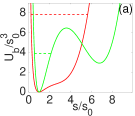
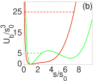
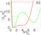
Figure 4 shows normalised functional forms of the pseudo-potential (6), which correspond to solutions plotted in the phase space panels. Dashed lines in each panel correspond to the initial condition for the red trajectory and the green trajectories shown in panels (d) of figures 1-3. The outermost nonlinear trajectories, plotted as a solid red line in panels (d) of figures 1-3 correspond to the pseudo-potentials with a single local minimum, which likely are transient states between the single and the double well potentials. The energy of the observed nonlinear fluctuations are still much higher than any local extrema or plateau visible in the red curve of figure 4(c). In the classification given in Hada these fluctuations were called algebraic soliton solutions. In contrast, the solid green trajectories of figures 1-3 represent solutions near the local equilibrium of a double-well potential. The pseudo-potential reflects the properties of the medium in which the wave propagates. The change of the potential may be interpreted as the feedback of nonlinear waves on the background plasma. This results in a double-well potential, a solution corresponding to a large limit in the phase speeds , however the available energy in the system can only sustain small amplitude oscillations (green trajectories), near one of the equilibrium points.
Conclusions. We presented the first explicit detection of nonlinear waves with frequencies higher than that of the ion cyclotron and have shown that these waves are consistent with analytical predictions and numerical solutions of the DNLS equation. The phase speed of the large amplitude nonlinear waves is approximately equal the local Alfvén speed. Obtained solutions are consistent with parallel propagating fast magnetosonic waves, given their sense of polarisation and previously obtained direction of propagation Narita03 . The impact of the nonlinear waves on the background plasma has been quantified by the change of the pseudo-potential, which shows a transition from a double well to a single well form. The presence of a double-well potential could, in principle, support a super-nonlinear wave Dubinov12 .
As these fluctuations are further advected towards the bow shock, they refract and their greater oblique propagation angle leads to faster steepening Hada . Thus the applicability of the DNLS evolution equation may depend on the distance from the origin of the fluctuations. Since the quasi-parallel component of plasma turbulence may be treated as interactions between multiple solitary nonlinear waves, further studies are needed to understand the temporal evolution of these fluctuations.
References
- (1) R. H. Cohen and R. S. Kulsrud, Phys. of Fluids, 17, 2215-2225 (1974), DOI:10.1063/1.1694695
- (2) V. E. Zakharov, 1972, Zh. Eksp. Teor. Fiz. 62, 1745, Sov. Phys. JETP 35, 908 (1972).
- (3) A. Hasegawa, Phys. Rev. A 1, 1746 (1970).
- (4) P. A. Robinson, Rev. Mod. Phys. 69, 507 (1997).
- (5) C. F. Kennel, B. Buti, T. Hada, R. Pellat, R., Phys. Fluids 31, 1949 (1988).
- (6) J. W. Belcher, and L. Davis Jr., J. Geophys. Res., 76, 3534 3563, doi:10.1029/JA076i016p03534 (1971).
- (7) R. P. Sharma, S. Sharma, and N. Gaur, J. Geophys. Res. Space Physics, 120, 6045 6054, doi: 10.1002/2015JA021215 (2015).
- (8) J. P. Eastwood, A. Balogh, E. A. Lucek, Ann. Geophys., 21, 1457 1465 (2003).
- (9) P. Kajdič, X. Blanco-Cano, E. Aguilar-Rodriguez, C. T. Russell, L. K. Jian, and J. G. Luhmann , J. Geophys. Res., 117, A06103, (2012) doi:10.1029/2011JA017381.
- (10) A. R. Bell, Mon. Not. R. Astron. Soc., 182, 147 (1978).
- (11) J. He, E. Marsch, C. Tu, S. Yao and H. Tian, Astroph. J., 731, 85 (2011).
- (12) T. Kukutani and H. Ono, Journal of the Physical Society of Japan, 26 (1969).
- (13) A. Rogister, Physics of Fluids 14, 2733 (1971); doi: 10.1063/1.1693399
- (14) E. Mjolhus, Physica Scripta 40, 227 (1989).
- (15) Hada, T., Kennel, C. F., & Buti, B. 1989, J. Geophys. Res., 94, 65
- (16) B. Buti, B. T. Tsurutani, M. Neugebauer and B. E. Goldstein, Geophys. Res. Lett, 28, 1355-1358 (2001).
- (17) S. Ghosh, & K. Papadopoulos, Phys. Fluids, 30, 1371 (1987).
- (18) M. V. Medvedev, V. I. Shevchenko, P. H. Diamond, & V. L. Galinsky, Phys. Plasmas, 4, 1257 (1997).
- (19) E. Dubinin, K. Sauer and J. F. McKenzie, Journal of Plasma Physics, 69, 305-330 doi:10.1017/S0022377803002319 (2003).
- (20) Sauer, K., E. Dubinin, and J. F. McKenzie, Geophys. Res. Lett., 29, 2226, doi:10.1029/2002GL015771 (2002).
- (21) D. Burgess, Adv. Space Res., 20, 673 (1997).
- (22) L. A. Selzer, B. Hnat, K. T. Osman, V. M. Nakariakov, J. P. Eastwood, and D. Burgess, The Astroph. J. Lett. 788, (2014).
- (23) S. D. Bale, P. J. Kellogg, D. E. Larsen, R. P. Lin, K. Goetz, R. P. Lepping, Geophys. Res. Lett., 25, 1944-8007, 10.1029/98GL02111 (1998).
- (24) D. B. Graham , Y. V. Khotyaintsev, A. Vaivads, and M. André, Geophys. Res. Lett., 42, 215 224 (2015); doi:10.1002/2014GL062538.
- (25) A. E. Dubinov and M. A. Sazonkin, Journal of Experimental and Theoretical Physics, Vol. 111, 865 876 (2011).
- (26) Y. Narita, K.-H. Glassmeier, S. Schafer, U. Motschmann, K. Sauer, I. Dandouras, K.-H. Fornacon, E. Georgescu, H. and Réme, Geophys. Res. Lett., 30, 1710 (2003); doi:10.1029/2003GL017432
- (27) A. Balogh, et al., Space Sci. Rev. 79, 65-91, (1997).
- (28) H. Réme, Ann. Geophys., 19, 1303–1354 (2001).
- (29) B. U. Sonnerup, M. & Scheible, (1998). Analysis Methods for Multi-Spacecraft Data Gotz Paschmann and Patrick W. Daly (Eds.), ISSI Scientific Report SR-001 (Electronic edition 1.1)
- (30) N. E. Huang, Z. Shen, S. R. Long, M. C. Wu, H. H. Shih, Q. Zheng, N.-C. Yen, C. C. Tung, H. H. Liu, Proceedings of the Royal Society of London Series A. 454, 903-998 (1998).
- (31) Z. Wu and N. E. Huang, Adv. Adapt. Data Anal. 01, 1 (2009). DOI: 10.1142/S1793536909000047
- (32) V. M. Nakariakov et al., Space Sci. Rev. (2016); DOI: 10.1007/s11214-015-0233-0
- (33) S. J. Schwartz, D. Burgess, Geophys. Res. Lett., 18, 1944–8007, 10.1029/91GL00138 (1991).
- (34) A. E. Dubinov, D. Y. Kolotkov and M. A. Sazonkin, Plasma Physics Reports, 38, 833 844 (2012).