Magnetic susceptibility of the QCD vacuum in a nonlocal SU(3) PNJL model

Abstract

The magnetic susceptibility of the QCD vacuum is analyzed in the framework of a nonlocal SU(3) Polyakov-Nambu-Jona-Lasinio model. Considering two different model parametrizations, we estimate the values of the $u$ and $s$-quark tensor coefficients and magnetic susceptibilities and then we extend the analysis to finite temperature systems. Our numerical results are compared to those obtained in other theoretical approaches and in lattice QCD calculations.

I Introduction

One of the most interesting features of quantum chromodynamics (QCD) is the nontrivial structure of its vacuum. This is clearly reflected on the vacuum expectation values of scalar quark condensates $\langle\bar{\psi}_{f}\psi_{f}\rangle$, which do not vanish at zero temperature and density. Light quark condensates are usually taken as order parameters related to the spontaneous breakdown of chiral symmetry, which can be regarded as one of the most important aspects of low energy strong interaction physics. Now, in order to get a more profound knowledge of the QCD vacuum it is interesting to study hadronic systems in the presence of external sources. In particular, it is seen that a constant external electromagnetic field induces the existence of other nonvanishing condensates, which describe the response of the vacuum to the source. We will concentrate here in the vacuum expectation value (VEV) of the tensor polarization operator $\langle\bar{\psi}\,\sigma_{\mu\nu}\,\psi\rangle$, where $\sigma_{\mu\nu}=i[\gamma_{\mu},\gamma_{\nu}]/2$ is the relativistic spin operator. In general, to leading order in the external field, for each quark flavor $f$ one has

$$\langle\bar{\psi}_{f}\,\sigma_{\mu\nu}\,\psi_{f}\rangle_{A}\ =\ q_{f}F_{\mu\nu}\,\tau_{f}\ ,$$ (1)

where $F_{\mu\nu}$ is the field strength tensor, $q_{f}$ is the quark electric charge and $\tau_{f}$ is the so-called tensor coefficient. The subindex $A$ indicates that the VEV is taken in the presence of an external electromagnetic field $A^{\mu}$. It is also usual to introduce the parameters $\chi_{f}$, defined by

$$\tau_{f}=\chi_{f}\;\langle\bar{\psi}_{f}\psi_{f}\rangle\ .$$ (2)

In the literature $\chi_{f}$ is frequently referred to as the magnetic susceptibility of the quark condensate, for a quark of flavor $f$. However, notice that it only constitutes the spin contribution to the total magnetic susceptibility. The quantity $\chi_{f}$ was first introduced in the context of QCD sum rules Ioffe:1983ju . Later it was noted that it is also relevant for the analysis of the muon anomalous magnetic moment Czarnecki:2002nt and for the description of several processes involving real photons, such as dijet production Braun:2002en and radiative decays Aliev:1999tq ; Ball:2003fq ; Colangelo:2005hv ; Rohrwild:2007yt .

Previous calculations of $\tau_{f}$ and/or $\chi_{f}$ for light and strange quark flavors have been carried out using QCD sum rules Belyaev:1984ic ; Balitsky:1985aq ; Ball:2002ps , in the holographic approach Bergman:2008sg ; Gorsky:2009ma , using the operator product expansion in the instanton liquid model and chiral effective models Kim:2004hd ; Dorokhov:2005pg ; Goeke:2007nc , using zero-modes of the Dirac operator Ioffe:2009yi , and in low-energy models of QCD such as the quark-meson model and the Nambu-Jona-Lasinio (NJL) model Frasca:2011zn . In addition, results from three-flavor lattice QCD (LQCD) simulations have become available recently Bali:2012jv . These include not only estimates at zero temperature but also at temperatures in the region of the chiral crossover transition. This has motivated the corresponding analysis carried out in Ref. Nam:2013wja within an effective SU(2) chiral effective model. The aim of the present work is to extend these studies further by considering the so-called nonlocal Polyakov-Nambu-Jona-Lasinio (nlPNJL) models Blaschke:2007np ; Contrera:2007wu ; Hell:2008cc ; Contrera:2009hk ; Hell:2009by , in which quarks move in a background color field and interact among themselves through covariant nonlocal chirally symmetric four-point couplings. These approaches, which can be considered as improvements over the (local) PNJL model Meisinger:1995ih ; Fukushima:2003fw ; Megias:2004hj ; Ratti:2005jh ; Roessner:2006xn ; Mukherjee:2006hq ; Sasaki:2006ww , offer a common framework to study both the chiral restoration and deconfinement transitions. In fact, the nonlocal character of the interactions arises naturally in the context of several successful approaches to low-energy quark dynamics Schafer:1996wv ; RW94 . Moreover, the presence of nonlocal form factors leads to a momentum dependence in light quark propagators that, under an appropriate choice of parameters Noguera:2008 ; Noguera:2005ej , is shown to be consistent with the corresponding LQCD results bowman ; Parappilly:2005ei ; Furui:2006ks .

The article is organized as follows. The theoretical framework is presented in Sect. II: in Sect. II.A we describe the model and quote the analytical expression for the tensor coefficients $\tau_{f}$, and this is extended to finite temperature in Sect. II.B, where Polyakov-loop potentials are introduced; then in Sect. II.C we discuss the model parametrizations to be considered. Sect. III is devoted to present our numerical results, which are compared with those obtained in other theoretical schemes and in LQCD calculations. Our conclusions are sketched in Sect. IV. We also include three appendices. In Appendix A we provide some details about the calculation of mean field values in our model, while in Appendix B we describe our regularization prescription for the tensor coefficients. Finally, in Appendix C possible alternative calculations of the tensor coefficients in the NJL model are discussed.

II Formalism

II.1 Magnetic susceptibility in a SU(3)_f nonlocal chiral quark model

As stated, we consider here a three-flavor nonlocal Nambu-Jona-Lasinio (nlNJL) model Scarpettini:2003fj ; Carlomagno:2013ona . We will work in Euclidean space, where the corresponding action is given by

$$S_{E} = \int d^{4}x\ \left\{\bar{\psi}(x)(-i\not{\partial}+\hat{m})\psi(x)-\frac{G}{2}\left[j_{a}^{S}(x)j_{a}^{S}(x)+j_{a}^{P}(x)j_{a}^{P}(x)+j^{\,r}(x)j^{\,r}(x)\right]\right.$$ (3)

$$\left.-\,\frac{H}{4}\,A_{abc}\left[j_{a}^{S}(x)j_{b}^{S}(x)j_{c}^{S}(x)-3j_{a}^{S}(x)j_{b}^{P}(x)j_{c}^{P}(x)\right]\right\}\ .$$

Here $\psi(x)$ is the $N_{f}=3$ fermion triplet $\psi=(u\ d\ s)^{T}$, and $\hat{m}={\rm diag}(m_{u},m_{d},m_{s})$ is the current quark mass matrix. We consider the isospin symmetry limit, assuming $m_{u}=m_{d}$. The model includes flavor mixing through the ’t Hooft-like term driven by the coupling constant $H$, in which the SU(3) symmetric constants $A_{abc}$ are defined by

$$A_{abc}\ =\ \frac{1}{3!}\,\epsilon_{ijk}\,\epsilon_{mnl}(\lambda_{a})_{im}\,(\lambda_{b})_{jn}\,(\lambda_{c})_{kl}\ ,$$ (4)

where $\lambda_{a}$, $a=0,\dots,8$, are the standard eight Gell-Mann matrices plus $\lambda_{0}=\sqrt{2/3}\,\mathbf{1}_{3\times 3}$. The fermion currents in Eq. (3) are given by

$$j_{a}^{S}(x) = \int d^{4}z\;\mathcal{G}(z)\,\bar{\psi}\left(x+\frac{z}{2}\right)\lambda_{a}\psi\left(x-\frac{z}{2}\right)\ ,$$

$$j_{a}^{P}(x) = \int d^{4}z\;\mathcal{G}(z)\,\bar{\psi}\left(x+\frac{z}{2}\right)i\lambda_{a}\gamma_{5}\psi\left(x-\frac{z}{2}\right)\ ,$$

$$j^{\,r}(x) = \int d^{4}z\;\mathcal{F}(z)\,\bar{\psi}\left(x+\frac{z}{2}\right)\frac{i\overleftrightarrow{\not{\partial}}}{2\kappa}\psi\left(x-\frac{z}{2}\right)\ ,$$ (5)

where $\mathcal{G}(z)$ and $\mathcal{F}(z)$ are covariant form factors responsible for the nonlocal character of the interactions. Notice that the relative weight of the interaction term that includes the currents $j^{\,r}(x)$ is controlled by the parameter $\kappa$. This coupling leads to quark wave function renormalization (WFR).

In what follows we will work within the mean field approximation (MFA). In momentum space, the effective quark propagators can be expressed as

$$S_{f}(p)=\frac{Z(p)}{-\not{p}+M_{f}(p)}\ ,$$ (6)

where $f=u,d,s$ is the corresponding quark flavor, and $M_{f}(p)$ and $Z(p)$ stand for the (momentum dependent) effective mass and WFR, respectively. These are given by

$$M_{f}(p) = Z(p)\,\Big{[}m_{f}\,+\,\bar{\sigma}_{f}\,g(p)\Big{]}\ ,$$

$$Z(p) = \rule{0.0pt}{22.76228pt}\left[1\,-\,\frac{\bar{\zeta}}{\kappa}\,f(p)\right]^{-1}\ ,$$ (7)

where the functions $g(p)$ and $f(p)$ are the Fourier transforms of $\mathcal{G}(z)$ and $\mathcal{F}(z)$, while $\bar{\sigma}_{f}$ and $\bar{\zeta}$ are mean field values of scalar fields associated with the currents in Eq. (5), in a flavor basis. Details of the procedure to obtain these quantities are given in Appendix A.

Let us consider in this framework the tensor polarization operator. In the presence of an electromagnetic field $A^{\mu}$, the vacuum expectation value of this operator at the leading order in $A^{\mu}$ is given by

$$\langle\bar{\psi}_{f}(x)\;\sigma_{\mu\nu}\;\psi_{f}(x)\rangle_{A}\ =\ -\,q_{f}\int\frac{d^{4}p}{(2\pi)^{4}}\frac{d^{4}p\,^{\prime}}{(2\pi)^{4}}\ e^{i(p^{\prime}-p)\cdot x}A^{\alpha}(p-p\,^{\prime})\ \mbox{Tr}\left[\sigma_{\mu\nu}\,S_{f}(p)\ \Gamma_{f\alpha}(p,p\,^{\prime})\ S_{f}(p\,^{\prime})\right]\ ,$$ (8)

where $\Gamma_{f\alpha}(p,p\,^{\prime})$ stands for the effective quark-photon vertex, and the trace is taken over Dirac and color indices. If the external magnetic field is spatially uniform, the electromagnetic field can be written as $A^{\mu}(x)=(-1/2)F^{\mu\nu}x_{\nu}$, therefore in momentum space one has

$$A^{\alpha}(p-p\,^{\prime})\ =\ -\frac{i}{2}\,F^{\alpha\beta}\,\frac{\partial}{\partial p\,^{\prime}_{\beta}}\left[(2\pi)^{4}\delta^{(4)}(p-p\,^{\prime})\right]\ .$$ (9)

In order to determine the couplings of dressed quarks to the electromagnetic field, one has to take into account that within the present nlNJL model the inclusion of gauge interactions implies not only a change in the kinetic terms in the Lagrangian (through the usual covariant derivative) but also a parallel transport of the fermion fields entering the nonlocal currents in Eq. (5). As discussed in Ref. Noguera:2005ej , the effective quark-photon vertex can be written as

$$\Gamma_{f}^{\alpha}(p,p\,^{\prime}) = \frac{1}{2}\left[\frac{1}{Z(p)}+\frac{1}{Z(p\,^{\prime})}\right]\gamma^{\alpha}+\frac{1}{2}\left[\frac{1}{Z(p)}-\frac{1}{Z(p\,^{\prime})}\right]\frac{(p+p\,^{\prime})^{\alpha}}{p^{2}-p\,^{\prime 2}}\,(\not{p}+\not{p}\,^{\prime})$$ (10)

$$-\left[\frac{M_{f}(p)}{Z(p)}-\frac{M_{f}(p\,^{\prime})}{Z(p\,^{\prime})}\right]\frac{(p+p\,^{\prime})^{\alpha}}{p^{2}-p\,^{\prime 2}}+\nu^{(1)}_{f}(p,p\,^{\prime})\ T_{1}^{\alpha}+\nu^{(2)}(p,p\,^{\prime})\ T_{2}^{\alpha}\ ,$$

where

$$\nu^{(1)}_{f}(p,p\,^{\prime}) = -\,\frac{1}{p\,^{\prime\,2}-p^{2}}\ \int_{-1}^{1}d\lambda\ \lambda\left[\frac{d}{dp^{2}}\frac{M_{f}(p)}{Z(p)}\right]_{p=\bar{p}-\lambda k/2}\ ,$$

$$\nu^{(2)}(p,p\,^{\prime}) = \frac{1}{p\,^{\prime\,2}-p^{2}}\ \int_{-1}^{1}d\lambda\ \lambda\left[\frac{d}{dp^{2}}\frac{1}{Z(p)}\right]_{p=\bar{p}-\lambda k/2}\ ,$$

$$T_{1}^{\alpha}(p,p\,^{\prime}) = p^{\alpha}\,(p\,^{\prime}\cdot k)-p\,^{\prime\alpha}\,(p\cdot k)\ ,$$

$$T_{2}^{\alpha}(p,p\,^{\prime}) = T_{1}^{\alpha}(p,p\,^{\prime})\,\frac{\not{p}+\not{p}\,^{\prime}}{2}\ ,$$ (11)

with $\bar{p}=(p+p\,^{\prime})/2$, $k=p\,^{\prime}-p$. The functions $\nu^{(1)}_{f}(p,p\,^{\prime})$ and $\nu^{(2)}(p,p\,^{\prime})$ arise from the parallel transport of fermion fields, which involves an integral over an arbitrary path ripka . The result in Eqs. (10-11) corresponds to the choice of a straight line path.

Then, taking into account the definition in Eq. (1), from Eqs. (8-11) the tensor coefficient is found to be given by

$$\tau_{f}\ =\ 4N_{c}\int\frac{d^{4}p}{(2\pi)^{4}}\ Z(p)\ \frac{M_{f}(p)-p^{2}M_{f}^{\prime}(p)}{\left[p^{2}+M_{f}(p)^{2}\right]^{2}}\ ,$$ (12)

where $M_{f}^{\prime}\equiv dM_{f}/dp^{2}$. Notice that this result does not depend on the functions $\nu^{(1)}_{f}(p,p\,^{\prime})$ and $\nu^{(2)}(p,p\,^{\prime})$, i.e. on the arbitrary path chosen for the gauge transformation carried out on fermion fields. It is also worth noticing that for finite current quark masses the integral in Eq. (12) is ultraviolet divergent, thus it has to be regularized. This can be accomplished by subtracting the corresponding value in the absence of interactions (see the discussion in Appendix B).

II.2 Extension to finite temperature

We will extend the analysis of the SU(3)_f nlNJL model introduced in the previous section to a system at finite temperature by using the standard Matsubara formalism. In addition, in order to account for confinement effects, we will include the coupling of fermions to the Polyakov loop (PL), assuming that quarks move on a constant color background field $\phi=ig\,\delta_{\mu 0}\,G^{\mu}_{a}\lambda^{a}/2$, where $G^{\mu}_{a}$ are the SU(3) color gauge fields. We will work in the so-called Polyakov gauge, in which the matrix $\phi$ is given a diagonal representation $\phi=\phi_{3}\lambda_{3}+\phi_{8}\lambda_{8}$, taking the traced Polyakov loop $\Phi=\frac{1}{3}{\rm Tr}\,\exp(i\phi/T)$ as an order parameter of the confinement/deconfinement transition. Since —owing to the charge conjugation properties of the QCD Lagrangian Dumitru:2005ng — the mean field traced Polyakov loop is expected to be a real quantity, and $\phi_{3}$ and $\phi_{8}$ are assumed to be real valued Roessner:2006xn , one has $\phi_{8}=0$, $\Phi=[1+2\cos(\phi_{3}/T)]/3$. In addition, we include effective gauge field self-interactions through a Polyakov-loop potential ${\cal U}\,[\Phi]$. The resulting scheme is usually denoted as a nonlocal Polyakov-Nambu-Jona-Lasinio (nlPNJL) model Blaschke:2007np ; Contrera:2007wu ; Contrera:2009hk ; Hell:2008cc ; Hell:2009by .

Concerning the PL potential, its functional form is usually based on properties of pure gauge QCD. In this work we consider three alternative forms that have been proposed in the literature. One possible ansatz is that based on the logarithmic expression of the Haar measure associated with the SU(3) color group integration. The corresponding potential is given by Roessner:2006xn

$$\frac{{\cal{U}}_{\rm log}(\Phi,T)}{T^{4}}\ =\ -\,\frac{1}{2}\,a(T)\,\Phi^{2}\;+\;b(T)\,\log\left(1-6\,\Phi^{2}+8\,\Phi^{3}-3\,\Phi^{4}\right)\ ,$$ (13)

where

$$a(T)=a_{0}+a_{1}\left(\dfrac{T_{0}}{T}\right)+a_{2}\left(\dfrac{T_{0}}{T}\right)^{2}\ ,\qquad b(T)=b_{3}\left(\dfrac{T_{0}}{T}\right)^{3}\ .$$ (14)

The parameters in these equations can be fitted to pure gauge lattice QCD calculations so as to properly reproduce the corresponding equation of state and Polyakov loop behavior. This leads to Roessner:2006xn

$$a_{0}=3.51\ ,\qquad a_{1}=-2.47\ ,\qquad a_{2}=15.2\ ,\qquad b_{3}=-1.75\ .$$ (15)

The values of $a_{i}$ and $b_{i}$ are constrained by the condition of reaching the Stefan-Boltzmann limit at $T\rightarrow\infty$ and by imposing the presence of a first-order phase transition at $T_{0}$, which is a further parameter of the model. In the absence of dynamical quarks, from lattice calculations one expects a deconfinement temperature $T_{0}=270$ MeV. However, it has been argued that in the presence of light dynamical quarks this temperature scale should be adequately reduced to about 210 and 190 MeV for the case of two and three flavors, respectively, with an uncertainty of about 30 MeV Schaefer:2007pw .

Besides the logarithmic form in Eq. (13), a widely used potential is that given by a polynomial function based on a Ginzburg-Landau ansatz Ratti:2005jh ; Scavenius:2002ru :

$$\frac{{\cal{U}}_{\rm poly}(\Phi,T)}{T^{4}}\ =\ -\,\frac{b_{2}(T)}{2}\,\Phi^{2}-\,\frac{b_{3}}{3}\,\Phi^{3}+\,\frac{b_{4}}{4}\,\Phi^{4}\ ,$$ (16)

where

$$b_{2}(T)=a_{0}+a_{1}\left(\dfrac{T_{0}}{T}\right)+a_{2}\left(\dfrac{T_{0}}{T}\right)^{2}+a_{3}\left(\dfrac{T_{0}}{T}\right)^{3}\ .$$ (17)

Here the reference temperature $T_{0}$ plays the same role as in the logarithmic potential in Eq. (13). Once again, the parameters can be fitted to pure gauge lattice QCD results so as to reproduce the corresponding equation of state and Polyakov loop behavior. Numerical values can be found in Ref. Ratti:2005jh .

Finally, we consider the so-called “improved” Polyakov loop potentials recently proposed in Ref. Haas:2013qwp , in which the full QCD potential ${\cal{U}}_{\rm glue}$ is related to a Yang-Mills potential ${\cal{U}}_{\rm YM}$:

$$\frac{{\cal{U}}_{\rm glue}(\Phi,t_{\rm glue})}{T^{4}}\ =\ \frac{{\cal{U}}_{\rm YM}[\Phi,t_{\rm YM}(t_{\rm glue})]}{T_{\rm YM}^{4}}\ ,$$ (18)

where

$$t_{\rm YM}(t_{\rm glue})\ =\ 0.57\,t_{\rm glue}\ =\ 0.57\left(\frac{T-T_{c}^{\rm glue}}{T_{c}^{\rm glue}}\right)\ .$$ (19)

The dependence of the Yang-Mills potential on the Polyakov loop $\Phi$ and the temperature $T_{YM}$ is taken from an ansatz such as those in Eq. (13) or (16), while for $T_{c}^{\rm glue}$ a preferred value of 210 MeV is obtained Haas:2013qwp .

Once the form of the effective action is established, the vacuum expectation value of the tensor polarization operator at finite temperature can be obtained by following a similar procedure as the one described in the previous subsection. One gets

$$\tau_{f}(T)\ =\ 4T\sum_{n=-\infty}^{\infty}\sum_{c=r,g,b}\int\frac{d^{3}p}{(2\pi)^{3}}\ Z(p_{nc})\,\frac{M_{f}(p_{nc})-p_{nc}^{2}\,M_{f}^{\prime}(p_{nc})}{\left[p_{nc}^{2}+M(p_{nc})^{2}\right]^{2}}\ ,$$ (20)

where $p_{nc}^{2}=[(2n+1)\pi T+\phi_{c}]^{2}+\vec{p}^{\;2}$, and $\phi_{c}$ is given by the relation $\phi=\textrm{diag}(\phi_{r},\phi_{g},\phi_{b})=\textrm{diag}(\phi_{3},-\phi_{3},0)$. In general, as in case of the $T=0$ expression in Eq. (12), it is seen that the integral in Eq. (20) is ultraviolet divergent. We regularize it by subtracting the $T=0$ divergent piece, which is equivalent to subtract a “free” contribution obtained from Eq. (20) in the limit $\bar{\sigma}_{u,s}=\bar{\zeta}=0$, and add this contribution written in a regularized form. Details are given in Appendix B.

II.3 Model parameters and form factors

In order to fully specify the model under consideration we need to fix the value of the five parameters it includes, namely the current quark masses $m_{u,s}$ and the coupling constants $G$, $H$, and $\kappa$. In addition, one has to specify the form factors ${\cal F}(z)$ and ${\cal G}(z)$ entering the nonlocal fermion currents [or, equivalently, the corresponding Fourier transforms $f(p)$ and $g(p)$]. Given the form factor functions, one can fix the model parameters so as to reproduce the observed meson phenomenology. Here, following Ref. Carlomagno:2013ona , we will consider two parametrizations, corresponding to two different functional forms for $f(p)$ and $g(p)$. The first one corresponds to the often used exponential behaviors

$$g(p)=\exp\left(-p^{2}/\Lambda_{0}^{2}\right)\ ,\qquad f(p)=\exp\left(-p^{2}/\Lambda_{1}^{2}\right)\ ,$$ (21)

which guarantee a fast ultraviolet convergence of the loop integrals. Note that the range of the nonlocality in each channel is determined by the parameters $\Lambda_{0}$ and $\Lambda_{1}$, which can be viewed as effective momentum cutoffs. In order to fix the parameters we have required the model to reproduce the phenomenological values of five physical quantities, namely the masses of the pseudoscalar mesons $\pi$, $K$ and $\eta^{\prime}$, the pion weak decay constant $f_{\pi}$ and the light quark condensate $\langle\bar{\psi}_{u}\psi_{u}\rangle$. In addition, on the basis of lattice QCD estimations Parappilly:2005ei , we have fixed the value of the quark WFR at zero momentum to be $Z(0)=0.7$.

The second parametrization considered here is based on the analysis in Ref. bowman , in which the effective mass $M_{u}(p)$ is written as

$$M_{u}(p)\ =\ m_{u}\,+\,\alpha_{m}\,f_{m}(p)\ ,$$ (22)

where

$$f_{m}(p)\ =\ \frac{1}{1+(p^{2}/\Lambda_{0}^{2})^{3/2}}\ .$$ (23)

From Eqs. (7) one has $\alpha_{m}=(m_{u}\bar{\zeta}/\kappa+\bar{\sigma}_{u})/(1-\bar{\zeta}/\kappa)$. For the wave function renormalization we use the parametrization Noguera:2005ej ; Noguera:2008

$$Z(p)\ =\ 1\,-\,\alpha_{z}\,f_{z}(p)\ ,$$ (24)

where

$$f_{z}(p)\ =\ \frac{1}{\left(1+p^{2}/\Lambda_{1}^{2}\right)^{5/2}}\ .$$ (25)

Here the new parameter $\alpha_{z}$ is given by $\alpha_{z}=-\bar{\zeta}/(\kappa-\bar{\zeta})$. The functions $f(p)$ and $g(p)$ can be now easily obtained from Eqs. (7), (22) and (24). As shown in Refs. Carlomagno:2013ona ; Noguera:2008 , for an adequate choice of parameters these functional forms can reproduce very well the momentum dependence of quark mass and WFR obtained in lattice calculations. We complete the model parameter fixing by taking as phenomenological inputs the values the of the pion, kaon and $\eta^{\prime}$ masses and the pion weak decay constant.

In Table I we quote the numerical values for the model parameters that we have obtained for the above-described form factor functions. In what follows, the parametrizations corresponding to Eqs. (21) and (22-25) will be referred to as parametrizations PI and PII, respectively.

	PI	PII
$m_{u}$ [MeV]	5.7	2.6
$m_{s}$ [MeV]	136	64.9
$G\Lambda_{0}^{2}$	23.64	16.65
$-H\Lambda_{0}^{5}\ \$	526	202.8
$\kappa$ [GeV]	4.36	8.218
$\Lambda_{0}$ [GeV]	0.814	0.795
$\Lambda_{1}$ [GeV]	1.032	1.510

Table 1: Model parameters for the form factors in Eqs. (21) (PI) and (22-25) (PII).

III Numerical results

Given the model parametrization we can solve the set of equations (A.3) and (A.4), which allow us to obtain the mean field values $\bar{\sigma}_{u,s}$ and $\bar{\zeta}$ at zero temperature, as described in App. A. Once these values are obtained it is straightforward to compute the quark condensates and the tensor coefficients for light and strange quark flavors, according to Eqs. (A.6) and (12). Our numerical results for parametrizations I and II are summarized in Table 2, where we also quote for comparison the corresponding estimates obtained within other models. Firstly we observe that our model, in accordance with other theoretical results, predicts a diamagnetic behavior for the QCD vacuum. In addition, for both parametrizations the values obtained for the $u-$tensor coefficient are found to be in very good agreement with the LQCD estimate. In the case of the light quark magnetic susceptibility we find some discrepancy between the results for PI and PII, which turn out to be above and below the LQCD estimate, respectively. The discrepancy can be explained by noting that the values for the light quark condensates for both parametrizations are also significantly different. In fact, this difference arises basically from the fact that for PI we have taken as input the phenomenological value $-\langle\bar{\psi}_{u}\,\psi_{u}\rangle^{1/3}=240$ MeV, which corresponds to a renormalization scale of about 1 GeV, while PII has been obtained through a fit to lattice data in Ref. Parappilly:2005ei for the effective quark propagator, which correspond to a higher momentum scale of 3 GeV. Regarding the $s-$tensor coefficient, we find that its value is more dependent on the chosen parametrization than in the case of $\tau_{u}$. When comparing with the quoted results of other models, it is seen that the prediction obtained from PII is the closest one to LQCD. In any case, it is important to point out that in general the various theoretical scenarios leading to the results presented in Table II consider different renormalization scales, therefore the comparison of numerical values should be taken with some care. Moreover, in the case of the predictions obtained within the local NJL model it is seen that the results are rather dependent on the calculation scheme. This is discussed in App. C, where we compare the values for $\tau_{u}$ arising from different regularization approaches. For comparison we include in Table 2 the results given by the calculation in Ref. Frasca:2011zn and those arising from an alternative approach that we refer to as “weak field propagator expansion” (WFPE), in which we have used the SU(3)_f NJL parametrization given in Ref. Hatsuda:1994pi .

		nlNJL		NJL	NJL∗	ILM	DS	LQCD
		PI	PII
$\mu$	[GeV]	0.814	3.0	0.627	0.631	0.85	0.4-0.7	2.0
$m_{u}$	[MeV]	5.7	2.6	5	5.5	5	0	3.5
$-\langle\bar{\psi}_{u}\,\psi_{u}\rangle^{1/3}$	[MeV]	240	316	253	247	260	251	269
$-\langle\bar{\psi}_{s}\,\psi_{s}\rangle^{1/3}$	[MeV]	198	341	$...$	267	$...$	$...$	250
$\tau_{u}$	[MeV]	38.2	44.6	69	25.8	40-45	28-33	40
$\tau_{s}$	[MeV]	9.7	30	$...$	19.8	6-10	$...$	53
$-\chi_{u}\ \$	[GeV-2]	2.77	1.42	4.3	1.72	2.5	1.7 -2.1	2.05 (0.09)
$-\chi_{s}\ \$	[GeV-2]	1.25	0.76	$...$	1.03	$...$	$...$	3.40 (1.40)

Table 2: Condensates and magnetic susceptibilities obtained in the present nlNJL model in comparison with other existing theoretical estimates: NJL corresponds to the NJL model calculation in Ref. Frasca:2011zn , NJL^∗ corresponds to a NJL model calculation based on what we call WFPE approach (see App. C), ILM to the instanton liquid model calculation in Ref. Kim:2004hd , DS to the Dyson-Schwinger calculation in Ref. Watson:2013ghq and LQCD to the lattice estimate in Ref. Bali:2012jv .

Let us now study the temperature dependence of the tensor coefficient in the various possible scenarios available for the parametrizations and Polyakov loop potentials discussed in the previous section. Our results for $\tau_{u}$ as a function of the temperature, using the regularization prescription discussed in App. B, are presented in Fig. 1. If the temperature is increased starting from $T=0$, for all cases under consideration it is seen that the tensor coefficient remains approximately constant up to some critical temperature, and then one finds a sudden drop, which is a signature of the restoration of the SU(2) chiral symmetry. Therefore, $\tau_{u}$ may be regarded as an approximate order parameter for the chiral restoration transition. In the upper panel of Fig. 1 we show the curves obtained within the present nlPNJL model for both parametrizations PI and PII (dashed and solid lines, respectively), considering the improved polynomial potential for the Polyakov loop. For comparison we also show the results from Ref. Kim:2004hd , obtained in the context of the instanton liquid model (ILM), as well as LQCD estimates from Ref. Bali:2012jv (dotted line and grey dashed band, respectively). Firstly we notice that ILM results predict that for low temperatures the tensor condensate becomes increased with respect to $\tau_{u}(0)$, while in our model it remains approximately constant up to the chiral transition region. In order to characterize the transition, we define the critical temperature $T_{c}$ as the temperature at which the function $\tau_{u}(T)$ has an inflection point. Following this definition we find for the case of the improved polynomial potential a critical temperature $T_{c}=158$ (160) MeV for PI (PII), while lattice results lead to $T_{c}^{\rm LQCD}\sim 162$ MeV Bali:2012jv . Moreover, we observe that at temperatures above the transition region the shape of the curves obtained within our model are in reasonable agreement with lattice calculations. On the other hand, the onset of the transition within nlPNJL models is found to be rather steep, thus the curve arising from the ILM seems to be more compatible with lattice results right below the critical temperature. In fact, this discrepancy between nlPNJL and LQCD estimates may be cured once the mesonic fluctuations are included in the Euclidean action Blaschke:2007np ; Hell:2008cc ; Hell:2009by ; Radzhabov:2010dd . This can be understood by noting that when the temperature is increased the light mesons should be excited before the quarks, and this would soften the behavior of the tensor coefficient at the onset of the transition. It is important to mention that the incorporation of mesonic corrections should not modify the critical temperatures.

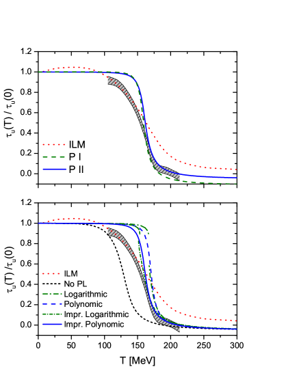
Figure 1: Normalized $u$-quark tensor coefficient vs. temperature for nonlocal PNJL models. Upper panel: results corresponding to the polynomial PL potential in Eq. (16), for parametrizations PI and PII. Lower panel: results corresponding to parametrization PII, for various PL potentials. For comparison, values obtained within the ILM Nam:2013wja (dotted lines) and results from LQCD Bali:2012jv (dashed grey bands) are also shown in both graphs.

Next, in the lower panel of Fig. 1 we show the curves for the tensor coefficient as function of the temperature for the nlPNJL model, considering various functional forms for the Polyakov loop potential. All results correspond to the lattice QCD-inspired parametrization PII. For comparison we include once again LQCD and ILM results, as well as a curve corresponding to the tensor coefficient in the nlNJL model without the coupling between the quarks and the Polyakov loop. In this last case (short-dashed line) it is observed that the transition temperature turns out to be too low in comparison with LQCD estimates, as it is indeed expected from previous calculations Contrera:2007wu . The graph shows that whereas different PL potentials give rise to different shapes for $\tau_{u}(T)$ at temperatures below the chiral transition, once the transition is surpassed the functions converge to a single curve that is in agreement with lattice estimates. In general it is seen that for the polynomial potentials the transition is smoother than in the case of the logarithmic ones, for which the transition is found to be of first order. Furthermore, for the improved potentials the curves tend to be smoother and the agreement with lattice results starts to occur already at the transition temperature. These general features on the comparison between the results of nlPNJL models and LQCD have also been observed within the study of chiral restoration, taking (as it is usually done) the quark condensates as order parameters of the transition Carlomagno:2013ona .

Finally, let us briefly discuss our results for the $s$-quark tensor coefficient and for other possible regularization prescriptions for $\tau_{u}(T)$ and $\tau_{s}(T)$. As stated, the results in Fig. 1 correspond to the prescription introduced in App. B, which is consistent with the usual regularization carried out at zero temperature. However, it may be argued that there are other possible regularization procedures. One possible option is to define tensor coefficients $\tau_{f}^{(\rm int)}$ by taking the expression in Eq. (B.2) without the addition of the free regularized terms, i.e. $\tau_{f}^{(\rm int)}(T)\equiv\tau_{f}^{(\rm reg)}(T)-\tau_{f}^{(0,\rm reg)}(T)$. This means to keep just the contribution of strong interaction dynamics to the tensor coefficients, hence in the limit of large temperatures one gets $\tau_{f}^{(\rm int)}(T)\to 0$ instead of the asymptotic free quark system behavior given by Eq. (B.5). Furthermore, another way to get rid of the free quark contribution at high temperatures is to define a “subtracted tensor coefficient” $\tau_{\rm sub}$ as

$$\tau_{\rm sub}(T)\ =\ \tau_{u}^{(\rm reg)}(T)-\frac{m_{u}}{m_{s}}\,\tau_{s}^{(\rm reg)}(T)+\frac{m_{u}\,N_{c}}{2\pi^{2}}\,\log\bigg{(}\frac{m_{s}}{m_{u}}\bigg{)}\ ,$$ (26)

which by construction also vanishes at large $T$ [see Eq. (B.5)].

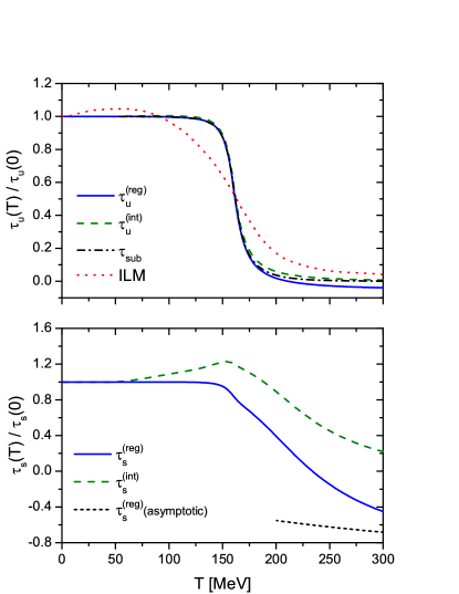
Figure 2: Normalized tensor coefficients vs. temperature for nlPNJL models. Results correspond to parametrization PII, improved polynomial PL potential and different regularization prescriptions. Upper panel: results corresponding to the $u$-quark tensor coefficients $\tau_{u}^{(\rm reg)}$ and $\tau_{u}^{(\rm int)}$ and the subtracted tensor coefficient $\tau_{\rm sub}$. For comparison values obtained within the ILM Nam:2013wja are also shown. Lower panel: results corresponding to the $s$-quark tensor coefficients $\tau_{s}^{(\rm reg)}$ and $\tau_{s}^{(\rm int)}$. The short dashed line shows the asymptotic behavior of $\tau_{s}^{(\rm reg)}(T)/\tau_{s}^{(\rm reg)}(0)$ at large temperatures.

The curves corresponding to $\tau_{u}^{\rm(reg)}(T)$, $\tau_{u}^{\rm(int)}(T)$ and $\tau_{\rm sub}(T)$, together with ILM results, are shown in the upper panel of Fig. 2. In all cases the results are normalized to the values at $T=0$, and correspond to parametrization PII and the improved PL potential discussed in Sect. II.B. For temperatures below the transition, it is found that $\tau_{u}^{\rm(reg)}(T)$ and $\tau_{\rm sub}(T)$ keep constant, while $\tau_{u}^{\rm(int)}$ (dashed line) shows some increase. This growth, barely noticeable in the figure, is in any case negligible in comparison with that found in the case of the ILM. Then, at the transition region the shape of all three curves look very much alike, therefore it can be said that the transition features do not depend on the regularization prescription. At larger temperatures, as expected, the curves for $\tau_{u}^{\rm(int)}(T)$ and $\tau_{\rm sub}(T)$ are similar (in both cases the contribution of free quarks has been somehow excluded), while $\tau_{f}^{\rm(reg)}$ is governed by the logarithmic behavior given by Eq. (B.5). The curves corresponding to the $s$-quark tensor coefficients $\tau_{s}^{\rm(reg)}(T)$ and $\tau_{s}^{\rm(int)}(T)$ are shown in the lower panel of Fig. 2. As in the case of the $u$ quark, it is seen that $\tau_{s}^{\rm(reg)}$ remains approximately constant for low $T$, starting to decrease at about the chiral transition critical temperature. However, we find that the slope is not so pronounced as in the case of $\tau_{u}$. At large temperatures the curve approaches the asymptotic logarithmic behavior, shown by the short-dashed line in the figure. On the other hand, the behavior of $\tau_{s}^{\rm(int)}(T)$ is quite different, showing a significant increase at temperatures below the transition and then a relatively slow descent. Thus, it is seen that even if the behavior of the $s$-quark tensor coefficient reflects the chiral restoration, it cannot be taken as a suitable order parameter in order to determine the critical transition temperature.

IV Summary and conclusions

In this work we have investigated the magnetic susceptibility of the QCD vacuum in the framework of a nonlocal SU(3) Polyakov-Nambu-Jona-Lasinio model.

Firstly we have considered the situation at vanishing temperature. We have found that the values for the $u$-quark tensor coefficient $\tau_{u}$ obtained within our model for parameterizations I and II are similar to each other, the results being in good agreement with estimates from lattice QCD and instanton liquid model calculations. On the other hand, these values are somewhat above the result obtained within a Dyson-Schwinger approach and clearly below the value arising from the NJL model calculation of Ref. [17]. It should be taken into account, however, that —as discussed in App. C— NJL model results are quite dependent on the way in which the calculation is performed. For the the corresponding $u$-quark magnetic susceptibilities we find some discrepancy between the results arising from our parametrizations I and II. This can be understood by noting that the values for the respective chiral condensates are also different to each other, which, in turn, is related to the fact that the parametrizations correspond to different momentum scales. In the case of the $s$-quark quantities our predictions turn out to be in general more dependent on the chosen parametrization. It should be noticed that lattice QCD estimates are also subject to larger uncertainties in this case.

Concerning the results at finite temperature we find that the tensor coefficient $\tau_{u}$ remains approximately constant up to a critical temperature, at which there is a sudden drop that can be clearly identified with the restoration of the SU(2) chiral symmetry. The curves are found to be similar for different regularization prescriptions. The stability observed at low temperatures differs from the behavior predicted in the context of the instanton liquid model, which shows a noticeable bump in that region. As occurs for other quantities (e.g. the scalar quark condensates) in the framework of nlPNJL models at the mean field level, we notice that at the onset of the chiral transition the behavior of the tensor coefficient is rather steep in comparison with lattice QCD estimates. This discrepancy is expected to be cured once meson fluctuations are included in the calculation. In any case, these corrections should not modify the behavior of the tensor coefficient above the transition, which is found to be in good agreement with lattice QCD results.

Appendix A: Mean field approximation and gap equations at $T=0$

Details on how to deal with the action in Eq. (3) at the mean field level can be found e.g. in Ref. Carlomagno:2013ona . For the reader’s convenience, in this appendix we sketch just the main details. We start by performing a standard bosonization of the fermionic theory, introducing scalar fields $\sigma_{a}(x)$, $\zeta(x)$ and pseudoscalar fields $\pi_{a}(x)$, together with auxiliary fields ${\cal S}_{a}(x)$, ${\cal R}(x)$ and ${\cal P}_{a}(x)$, with $a=0,\dots,8$. Now we follow the stationary phase approximation, replacing the path integral over the auxiliary fields by the corresponding argument evaluated at the minimizing values $\tilde{\cal S}_{a}$, $\tilde{\cal R}$ and $\tilde{\cal P}_{a}$. Next, we consider the MFA, in which the scalar and pseudoscalar fields are expanded around their vacuum expectation values:

$$\sigma_{a}(x)=\bar{\sigma}_{a}+\delta\sigma_{a}(x)\ ,\qquad\zeta(x)=\bar{\zeta}+\delta\zeta(x)\ ,\qquad\pi_{a}(x)=\delta\pi_{a}(x)\ .$$ (A.1)

We have assumed that pseudoscalar mean field values vanish, owing to parity conservation. Moreover, for the scalar fields only $\bar{\sigma}_{0,8}$ and $\bar{\zeta}$ can be different from zero due to charge and isospin symmetries. For the neutral fields ($a=0,3,8$) it is convenient to change to a flavor basis, $\sigma_{a},\pi_{a}\to\sigma_{f},\pi_{f}$, where $f=u,d,s$, or equivalently $f=1,2,3$. Then, the mean field action reads

$$\frac{S_{E}^{\,\mbox{\tiny MFA}}}{V^{(4)}} = 2\,N_{c}\sum_{f}\int\dfrac{d^{3}p}{(2\pi)^{3}}\;\log\left[\dfrac{Z(p)^{2}}{p^{2}+M_{f}(p)^{2}}\right]$$ (A.2)

$$-\left(\bar{\zeta}\,\bar{\cal R}+\dfrac{G}{2}\,\bar{\cal R}^{2}+\dfrac{H}{4}\,\bar{\cal S}_{u}\,\bar{\cal S}_{d}\,\bar{\cal S}_{s}\right)-\dfrac{1}{2}\,\sum_{f}\left(\bar{\sigma}_{f}\bar{\cal S}_{f}+\dfrac{G}{2}\,\bar{\cal S}_{f}^{2}\right)\ ,$$

where $N_{c}$ is the number of colors, and $\bar{\cal S}_{f}$ and $\bar{\cal R}$ stand for the values of $\tilde{\cal S}_{f}$ and $\tilde{\cal R}$ within the MFA, respectively. The functions $M_{f}(p)$ and $Z(p)$, given by Eqs. (7), correspond to the momentum-dependent effective masses and WFR of quark propagators $S_{f}(p)$ in Eq. (6).

By minimizing the mean field action in Eq. (A.2) one gets the set of coupled gap equations

$$\bar{\sigma}_{u}+G\bar{\cal S}_{u}+\frac{H}{2}\bar{\cal S}_{d}\bar{\cal S}_{s} = 0\ ,$$

$$\bar{\sigma}_{d}+G\bar{\cal S}_{d}+\frac{H}{2}\bar{\cal S}_{s}\bar{\cal S}_{u} = 0\ ,$$

$$\bar{\sigma}_{s}+G\bar{\cal S}_{s}+\frac{H}{2}\bar{\cal S}_{u}\bar{\cal S}_{d} = 0\ ,$$ (A.3)

plus an extra equation arising from the $j^{\,r}(x)$ current-current interaction,

$$\bar{\zeta}+G\bar{\cal R}=0\ .$$ (A.4)

The mean field values $\bar{\cal S}_{f}$ and $\bar{\cal R}$ in these equations are given by

$$\bar{\cal S}_{f} = -\,8N_{c}\int\frac{d^{4}p}{(2\pi)^{4}}\ g(p)\;\frac{Z(p)\,M_{f}(p)}{p^{2}+M_{f}(p)^{2}}\ \,,\qquad f=u,d,s\;,$$

$$\bar{\cal R} = \frac{4N_{c}}{\kappa}\int\frac{d^{4}p}{(2\pi)^{4}}\ p^{2}\,f(p)\;\sum_{f=1}^{3}\;\frac{Z(p)}{p^{2}+M_{f}(p)^{2}}\ \,.$$ (A.5)

Thus, for a given set of model parameters and form factors, from Eqs. (7) and (A.3-A.5) one can numerically obtain the mean field values $\bar{\sigma}_{f}$ and $\bar{\zeta}$.

The quark-antiquark condensates $\langle\bar{\psi}_{f}\,\psi_{f}\rangle$ can be now easily calculated by taking the derivative of the Euclidean mean field action with respect to the current quark masses. One gets

$$\langle\bar{\psi}_{f}\,\psi_{f}\rangle\ =\ -\,4N_{c}\int\frac{d^{4}p}{(2\pi)^{4}}\ \left[\frac{M_{f}(p)}{p^{2}+M_{f}(p)^{2}}-\frac{m_{f}}{p^{2}+m_{f}^{2}}\right]\ \,,$$ (A.6)

where we have subtracted a “free quark condensate” in order to regularize the otherwise divergent momentum integral.

Appendix B: Regularization of the tensor coefficient

As in the case of the quark condensate, the expression for the tensor coefficient in Eq. (12) can be regularized by subtracting a “free” $T=0$ contribution obtained in the limit $\bar{\sigma}_{u,s}=\bar{\zeta}=0$ (see e.g. Ref. Kim:2004hd ):

$$\tau_{f}^{\rm(reg)}\ =\ 4N_{c}\int\frac{d^{4}p}{(2\pi)^{4}}\ \bigg{\{}Z(p)\ \frac{M_{f}(p)-p^{2}M_{f}^{\prime}(p)}{\left[p^{2}+M_{f}(p)^{2}\right]^{2}}\ -\frac{m_{f}}{\big{(}p^{2}+m_{f}^{2}\big{)}^{2}}\bigg{\}}\ .$$ (B.1)

In the same way, for the case of a system at finite temperature $T$ we regularize the divergent integral in Eq. (20) by subtracting a finite temperature contribution in which $\bar{\sigma}_{u,s}=\bar{\zeta}=0$. Then, in order to recover the proper finite $T$ behavior at large $T$, we add this contribution after subtracting the $T=0$ divergent piece as in Eq. (B.1). Thus, using the same definitions as in Eq. (20), we have

$$\tau_{f}^{\rm(reg)}(T) = 4T\sum_{n=-\infty}^{\infty}\sum_{c=r,g,b}\int\frac{d^{3}p}{(2\pi)^{3}}\ \bigg{\{}Z(p_{nc})\,\frac{M_{f}(p_{nc})-p_{nc}^{2}\,M_{f}^{\prime}(p_{nc})}{\left[p_{nc}^{2}+M(p_{nc})^{2}\right]^{2}}$$ (B.2)

$$\ -\ \frac{m_{f}}{\big{(}p_{nc}^{2}+m_{f}^{2}\big{)}^{2}}\bigg{\}}\ +\ \tau_{f}^{(0,{\rm reg})}(T)\ \,,$$

where

$$\tau_{f}^{(0,{\rm reg})}(T)\ =\ 4T\sum_{n=-\infty}^{\infty}\sum_{c=r,g,b}\int\frac{d^{3}p}{(2\pi)^{3}}\ \frac{m_{f}}{\big{(}p_{nc}^{2}+m_{f}^{2}\big{)}^{2}}\ -4N_{c}\int\frac{d^{4}p}{(2\pi)^{4}}\ \frac{m_{f}}{\big{(}p^{2}+m_{f}^{2}\big{)}^{2}}\ \,.$$ (B.3)

The expression in Eq. (B.3) can be worked out, leading to

$$\tau_{f}^{(0,{\rm reg})}(T) = -\frac{m_{f}}{T^{3}}\int\frac{d^{3}p}{(2\pi)^{3}}\ \bigg{\{}\frac{1}{x_{f}^{2}}\bigg{[}\frac{1}{1+\cosh x_{f}}\;+\;\frac{8+4(3\Phi-1)\cosh x_{f}}{(3\Phi-1+2\cosh x_{f})^{2}}\bigg{]}$$ (B.4)

$$\ +\ \frac{6}{x_{f}^{3}}\;\frac{\Phi(1+2e^{-x_{f}})+e^{-2x_{f}}}{(1+e^{-x_{f}})\,({3\Phi-1+2\cosh x_{f}})}\bigg{\}}\ ,$$

where we have defined $x_{f}=\sqrt{p^{2}+m_{f}^{2}}/T$. In the limit of large temperature the behavior of the tensor coefficient is given by

$$\tau_{f}(T)|_{T\to\infty}\ \simeq\ -\,\frac{m_{f}\,N_{c}}{2\pi^{2}}\left[0.568+\log(T/m_{f})\right]\ .$$ (B.5)

Appendix C: Tensor coefficient in the NJL model

In this appendix we discuss the calculation of the tensor coefficient in the (local) NJL model. The value of $\tau_{u}$ that we have quoted in Table 2 corresponds to the SU(2) NJL model calculation carried out in Ref. Frasca:2011zn . There, the authors use the Ritus formalism Ritus:1972ky to derive an analytical expression for the VEV of the tensor polarization, and then they introduce a smooth form factor in order to regularize the divergent momentum integral. Our aim is to point out that there are alternative procedures that can be followed to calculate $\tau_{u}$ within the NJL model. In fact, it is seen that the numerical results turn out to be quite dependent on the way in which the calculation is performed.

Let us briefly describe the procedure followed in Ref. Frasca:2011zn . For consistency with this and other previous calculations, throughout this Appendix expressions are given in Minkowski space. The VEV of the tensor polarization operator is given by

$$\langle\bar{\psi}_{f}\,\sigma_{\mu\nu}\,\psi_{f}\rangle_{A}\ =\ -\,i\,{\rm Tr}\left[\sigma_{\mu\nu}\,S^{(A)}_{f}(x,x)\right]\ ,$$ (C.1)

where $S^{(A)}_{f}(x,x^{\prime})$ is the $f$-quark propagator (in coordinate space) in the presence of an external electromagnetic field $A_{\mu}$. For the particular case of a constant magnetic field $\vec{B}$ this propagator can be explicitly obtained. Within Ritus formalism, choosing $\vec{B}$ to be along the $z$ axis, one has

$$S^{(A)}_{f}(x,x^{\prime})_{\rm Rit}=\sum_{k=0}^{\infty}\frac{1}{(2\pi)^{4}}\int dp_{0}\,dp_{2}\,dp_{3}\ E_{P}(x)\;\Lambda_{k}\;\frac{1}{\gamma\cdot P-M_{f}(B)}\;\bar{E}_{P}(x^{\prime})\ ,$$ (C.2)

where $E_{P}(x)$ stands for the eigenfunction of a charged fermion of momentum $P^{\mu}$ in the magnetic field, and $\bar{E}_{P}(x)=\gamma_{0}\,E_{P}(x)^{\dagger}\,\gamma_{0}$. The index $k$ in the sum labels the Landau levels (LL), while $\Lambda_{k}$ is a projector in Dirac space that takes into account the LL degeneracy. The four-momentum $P^{\mu}$ is quantized according to

$$P_{\mu}\ =\ \big{(}p_{0}\,,\,0\,,\,{\rm sign}(q_{f})\sqrt{2k|q_{f}|B}\,,\,p_{3}\big{)}\ ,$$ (C.3)

where $q_{f}$ denotes the quark electric charge. Replacing the propagator in Eq. (C.2) into Eq. (C.1), a straightforward calculation shows that for our choice of magnetic field orientation the 12 component of the tensor is the only one that has a nonvanishing VEV. One has

$$\langle\bar{\psi}_{f}\,\sigma_{12}\,\psi_{f}\rangle_{A,{\rm Rit}}\ =\ N_{c}\frac{q_{f}B}{2}\int\frac{dp_{0}\,dp_{3}}{(2\pi)^{2}}\;\frac{i}{p_{0}^{2}-p_{3}^{2}-M_{f}(B)^{2}}\ ,$$ (C.4)

where the integral over $p_{2}$ has been performed. It is worth noticing that only the lowest LL (i.e. that corresponding to $k=0$) contributes to this VEV. Now, this expression is divergent and needs to be regularized. In Ref. Frasca:2011zn this has been achieved by introducing at this stage a cutoff function $U_{\Lambda}(|\vec{p}|)$ that depends only on the spatial components of the momentum, $\Lambda$ being a (three-momentum) cutoff scale. Following this procedure and performing the integral over $p_{0}$ one immediately obtains the expression in Eq. (17) of Ref. Frasca:2011zn . Expanding up to leading order in $B$, and noting that $F^{12}=-B$, one gets within this method an explicit expression for $\tau_{f}$, namely

$$\tau_{f}\ =\ \frac{N_{c}\,M_{f}}{2\pi^{2}}\ I_{\rm Rit}(M_{f}/\Lambda)\ ,$$ (C.5)

where

$$I_{\rm Rit}(x)\ =\ \int_{0}^{\infty}dy\ \frac{U_{\Lambda}\left(\Lambda y\right)}{\sqrt{y^{2}+x^{2}}}\ .$$ (C.6)

In Ref. Frasca:2011zn the particular form

$$U^{\rm Lor5}_{\Lambda}(p)\ =\ \frac{1}{1+(p/\Lambda)^{2N}}\ ,\qquad N=5\ ,$$ (C.7)

was used for numerical calculations. Alternatively, one can use a simple sharp cutoff function $U^{\rm SC}_{\Lambda}\left(p\right)=\theta\left(\Lambda-p\right)$, which leads to

$$I^{\rm SC}_{\rm Rit}(x)\ =\ \log\left[\frac{1+\sqrt{1+x^{2}}}{x}\right]\$$ (C.8)

(we have included the upper index SC to stress that it corresponds to the particular case in which $U_{\Lambda}(p)$ is a sharp cutoff function).

Let us consider now an alternative way to proceed based on the so-called Schwinger proper-time representation of the fermion propagator Schwinger:1951nm . As expected, once again it is seen that only the VEV of the 12 component of the tensor is nonvanishing. In this case one gets for this VEV the expression

$$\langle\bar{\psi}_{f}\,\sigma_{12}\,\psi_{f}\rangle_{A,{\rm Sch}}\ =\ -N_{c}\frac{q_{f}B}{4\pi^{2}}\int_{0}^{\infty}\frac{ds}{s}\exp\left[-sM_{f}^{2}(B)\right]\ ,$$ (C.9)

which as in the previous case needs to be regularized. As is customary when one uses the proper-time approach, we perform the regularization by replacing the lower limit of the integral by $1/\Lambda^{2}$. Expanding up to leading order in $B$ we get in this way

$$\tau_{f}\ =\ \frac{N_{c}\,M_{f}}{2\pi^{2}}\,I_{\rm Sch}(M_{f}/\Lambda)\ ,$$ (C.10)

where

$$I_{\rm Sch}(x)\ =\ \frac{1}{2}\,E_{1}(x)\ ,\qquad E_{n}(x)\ \equiv\ \int_{1}^{\infty}\;ds/s^{n}\,\exp(-sx)\ .$$ (C.11)

Finally, a yet alternative way to proceed is to follow the steps discussed in Sec. II.A, in which we consider from the beginning the expansion of the tensor operator at first order in powers of the magnetic field [see Eq. (8)], ending up with Eq. (12). We refer to this approach as “weak field propagator expansion” (WFPE). In the case of the NJL model one has (in Minkowski space)

$$\langle\bar{\psi}_{f}\,\sigma_{\mu\nu}\,\psi_{f}\rangle_{A,{\rm WFPE}}\ =\ -\,i\,4N_{c}\,q_{f}\,F_{\mu\nu}\int\frac{d^{4}p}{(2\pi)^{4}}\frac{M_{f}}{(p^{2}-M_{f}^{2})^{2}}\ .$$ (C.12)

It is important to stress that this expression can also be obtained by considering the weak field limit of the fermion propagator in a constant magnetic field given e.g. in Refs. Chyi:1999fc ; Watson:2013ghq . As stated in Ref. Watson:2013ghq , it is crucial to carry out the infinite sum over Landau levels in order to obtain the proper form of the propagator. Contrary to the case of the nonlocal model discussed throughout Sect. II, the integral in Eq. (C.12) turns out to be divergent even in the chiral limit. By using a 3D sharp cutoff regularization one finds

$$\tau_{f}\ =\ \frac{N_{c}M_{f}}{2\pi^{2}}\ I^{\rm SC}_{\rm WFPE}(M_{f}/\Lambda)\ ,$$ (C.13)

where

$$I_{\rm WFPE}^{\rm SC}(x)\ =\ \log\left[\frac{1+\sqrt{1+x^{2}}}{x}\right]-\frac{1}{\sqrt{1+x^{2}}}\ .$$ (C.14)

We can now compare the results for $\tau_{u}$ within the SU(2) NJL model that arise from the above discussed approaches. For this purpose, in all cases we fix the model parameters in such a way that the predicted values of $f_{\pi}$ and $m_{\pi}$ agree with the corresponding empirical values and the light quark condensate $\langle\bar{\psi}_{u}\,\psi_{u}\rangle^{1/3}$ has a phenomenologically reasonable value of $-250$ MeV. Our numerical results are given in Table 3.

	Rit (Lor5)	Rit (SC)	Sch	WFPE (SC)
$\tau_{u}$ [MeV]	70	70	42	28

Table 3: Numerical values for the tensor coefficient $\tau_{u}$ in the SU(2) NJL model

It is seen that our result for $\tau_{u}|_{\rm Rit}^{\rm Lor5}$ agrees with the value given in Ref. Frasca:2011zn , which has been quoted in Table 2, and it is also coincident with the result obtained within the Ritus approach for a sharp cutoff regularization function. On the other hand, this value is significantly different from those obtained following the Schwinger and WFPE approaches. This shows that the results for the tensor coefficient obtained within the local NJL model are quite dependent on the chosen regularization method, and have to be taken with care. In order to understand the origin of this dependence, it is interesting to compare with some detail the functions $I(x)$ defined above. Since the cutoff $\Lambda$ is expected to be larger than other scales in the problem, we can expand these functions for small values of $x$. We get

$$I_{\rm Rit}^{\rm LorN} = -\log x+\log 2+\frac{\pi}{4N}\csc\left(\frac{\pi}{N}\right)\ x^{2}+{\cal O}(x^{4})\ ,$$

$$I_{\rm Rit}^{\rm SC} = -\log x+\log 2+\frac{1}{4}\ x^{2}+{\cal O}(x^{4})\ ,$$

$$I_{\rm Sch} = -\log x-\frac{\gamma}{2}+\frac{1}{2}\ x^{2}+{\cal O}(x^{4})\ ,$$

$$I_{\rm WFPE}^{\rm SC} = -\log x+(\log 2-1)+\frac{3}{4}\ x^{2}+{\cal O}(x^{4})\ ,$$ (C.15)

where $\gamma$ is the Euler constant. As expected, all expressions have the same leading logarithmic contribution in the limit of small $x$, therefore the corresponding predictions for the tensor coefficient will be similar for $M_{f}/\Lambda\ll 1$. However, for realistic values of this ratio, the constant terms and the contributions carrying powers of $x$ become relevant. The differences between these terms shown in Eqs. (C.15) explain the differences between the numerical results in Table 3.

References

- (1) B. L. Ioffe and A. V. Smilga, Nucl. Phys. B 232, 109 (1984).
- (2) A. Czarnecki, W. J. Marciano and A. Vainshtein, Phys. Rev. D 67, 073006 (2003) Erratum: [Phys. Rev. D 73, 119901 (2006)].
- (3) V. M. Braun, S. Gottwald, D. Y. Ivanov, A. Schafer and L. Szymanowski, Phys. Rev. Lett. 89, 172001 (2002).
- (4) T. M. Aliev and M. Savci, Phys. Rev. D 60, 114031 (1999).
- (5) P. Ball and E. Kou, JHEP 0304, 029 (2003).
- (6) P. Colangelo, F. De Fazio and A. Ozpineci, Phys. Rev. D 72, 074004 (2005).
- (7) J. Rohrwild, JHEP 0709, 073 (2007).
- (8) V. M. Belyaev and Y. I. Kogan, Yad. Fiz. 40, 1035 (1984).
- (9) I. I. Balitsky, A. V. Kolesnichenko and A. V. Yung, Sov. J. Nucl. Phys. 41, 178 (1985) [Yad. Fiz. 41, 282 (1985)].
- (10) P. Ball, V. M. Braun and N. Kivel, Nucl. Phys. B 649, 263 (2003).
- (11) O. Bergman, G. Lifschytz and M. Lippert, JHEP 0805, 007 (2008).
- (12) A. Gorsky and A. Krikun, Phys. Rev. D 79, 086015 (2009).
- (13) H. C. Kim, M. Musakhanov and M. Siddikov, Phys. Lett. B 608, 95 (2005).
- (14) A. E. Dorokhov, Eur. Phys. J. C 42, 309 (2005).
- (15) K. Goeke, H. C. Kim, M. M. Musakhanov and M. Siddikov, Phys. Rev. D 76, 116007 (2007).
- (16) B. L. Ioffe, Phys. Lett. B 678, 512 (2009).
- (17) M. Frasca and M. Ruggieri, Phys. Rev. D 83, 094024 (2011).
- (18) G. S. Bali, F. Bruckmann, M. Constantinou, M. Costa, G. Endrodi, S. D. Katz, H. Panagopoulos and A. Schafer, Phys. Rev. D 86, 094512 (2012).
- (19) S. i. Nam, Phys. Rev. D 87, no. 11, 116003 (2013).
- (20) D. Blaschke, M. Buballa, A. E. Radzhabov and M. K. Volkov, Yad. Fiz. 71, 2012 (2008) [Phys. Atom. Nucl. 71, 1981 (2008)].
- (21) G. A. Contrera, D. Gomez Dumm and N. N. Scoccola, Phys. Lett. B 661, 113 (2008).
- (22) T. Hell, S. Roessner, M. Cristoforetti and W. Weise, Phys. Rev. D 79, 014022 (2009).
- (23) G. A. Contrera, D. Gomez Dumm and N. N. Scoccola, Phys. Rev. D 81, 054005 (2010).
- (24) T. Hell, S. Rossner, M. Cristoforetti and W. Weise, Phys. Rev. D 81, 074034 (2010).
- (25) P. N. Meisinger and M. C. Ogilvie, Phys. Lett. B 379, 163 (1996).
- (26) K. Fukushima, Phys. Lett. B 591, 277 (2004).
- (27) E. Megias, E. Ruiz Arriola and L. L. Salcedo, Phys. Rev. D 74, 065005 (2006).
- (28) C. Ratti, M. A. Thaler and W. Weise, Phys. Rev. D 73, 014019 (2006).
- (29) S. Roessner, C. Ratti and W. Weise, Phys. Rev. D 75, 034007 (2007).
- (30) S. Mukherjee, M. G. Mustafa and R. Ray, Phys. Rev. D 75, 094015 (2007).
- (31) C. Sasaki, B. Friman and K. Redlich, Phys. Rev. D 75, 074013 (2007).
- (32) T. Schafer and E. V. Shuryak, Rev. Mod. Phys. 70, 323 (1998).
- (33) C. D. Roberts and A. G. Williams, Prog. Part. Nucl. Phys. 33, 477 (1994); C. D. Roberts and S. M. Schmidt, Prog. Part. Nucl. Phys. 45, S1 (2000).
- (34) S. Noguera and N. N. Scoccola, Phys. Rev. D 78, 114002 (2008).
- (35) S. Noguera, Int. J. Mod. Phys. E 16, 97 (2007).
- (36) P. O. Bowman, U. M. Heller, and A. G. Williams, Phys. Rev. D 66, 014505 (2002); P. O. Bowman, U. M. Heller, D. B. Leinweber and A. G. Williams, Nucl. Phys. Proc. Suppl. 119, 323 (2003).
- (37) M. B. Parappilly, P. O. Bowman, U. M. Heller, D. B. Leinweber, A. G. Williams and J. B. Zhang, Phys. Rev. D 73, 054504 (2006).
- (38) S. Furui and H. Nakajima, Phys. Rev. D 73, 074503 (2006).
- (39) A. Scarpettini, D. Gomez Dumm and N. N. Scoccola, Phys. Rev. D 69, 114018 (2004).
- (40) J. P. Carlomagno, D. Gómez Dumm and N. N. Scoccola, Phys. Rev. D 88, no. 7, 074034 (2013).
- (41) G. Ripka, Quarks bound by chiral Fields, Oxford University Press (1997).
- (42) A. Dumitru, R. D. Pisarski and D. Zschiesche, Phys. Rev. D 72, 065008 (2005).
- (43) B. -J. Schaefer, J. M. Pawlowski and J. Wambach, Phys. Rev. D 76 , 074023 (2007); B. -J. Schaefer, M. Wagner and J. Wambach, Phys. Rev. D 81 , 074013 (2010).
- (44) O. Scavenius, A. Dumitru and J. T. Lenaghan, Phys. Rev. C 66, 034903 (2002).
- (45) L. M. Haas, R. Stiele, J. Braun, J. M. Pawlowski and J. Schaffner-Bielich, Phys. Rev. D 87, 076004 (2013).
- (46) P. Watson and H. Reinhardt, Phys. Rev. D 89, no. 4, 045008 (2014).
- (47) T. Hatsuda and T. Kunihiro, Phys. Rept. 247, 221 (1994).
- (48) A. E. Radzhabov, D. Blaschke, M. Buballa and M. K. Volkov, Phys. Rev. D 83, 116004 (2011).
- (49) V. I. Ritus, Annals Phys. 69, 555 (1972).
- (50) J. S. Schwinger, Phys. Rev. 82, 664 (1951).
- (51) T. K. Chyi, C. W. Hwang, W. F. Kao, G. L. Lin, K. W. Ng and J. J. Tseng, Phys. Rev. D 62, 105014 (2000).