Simultaneous Identification of Coefficient and Initial State for One-Dimensional Heat Equation from Boundary Control and Measurement

Abstract

In this paper, we consider simultaneous reconstruction of the diffusion coefficient and initial state for a one-dimensional heat equation through boundary control and measurement. The boundary measurement is known to make the system exactly observable, and both coefficient and initial state are shown to be identifiable by this measurement. By a Dirichlet series representation for observation, we can transform the problem into an inverse process of reconstruction of the spectrum and coefficients for Dirichlet series in terms of observation. This happens to be the reconstruction of spectral data for an exponential sequence with measurement error. This enables us to develop an algorithm based on the matrix pencil method in signal analysis. An error analysis is made for the proposed method. The numerical simulations are presented to verify the proposed algorithm.

Keywords:  Identification; identifiability; heat equation; matrix pencil method; error analysis.

AMS subject classifications:  35K05, 35R30, 65M32, 65N21, 15A22.

1 Introduction

It is recognized that many industrial controls are temperature control. The inverse heat conduction problem (IHCP) is one of the important control problems in science and engineering. Such kinds of problems usually arise in modeling and process control with heat propagation in thermophysics, chemical engineering, and many other industrial and engineering applications. In the last decades, there are various class of IHCPs having been investigated ranging from recovery of boundary heat flux [32]; estimation of medium parameters such as thermal conductivity coefficient [9, 18] and radiative coefficient [5, 6, 35]; recovery of spatial distribution of heat sources [19, 37]; and reconstruction of initial state distributions [35]. For many other aspects including numerical solutions of inverse problems for PDEs, we refer to monographs [14] and [15].

Most of the existing works, however, are devoted to single parameter identification. The simultaneous reconstruction of more than one different coefficients within a dynamical framework has not been sufficiently investigated, for which, to the best of our knowledge, only a few studies are available. In [3], the uniqueness and stability of determining both diffusion coefficient and initial condition from a measurement of the solution at a positive time and on an arbitrary part of the boundary for a heat equation are discussed. In [5] uniqueness and stability estimate of an inverse problem for a parabolic equation, where simultaneously determination of heat radiative coefficient, the initial temperature, and a boundary coefficient from a temperature distribution measured at a positive moment is considered. In [32], a numerical method is presented to determine both initial value and boundary value at one end from the discrete observation data at the other end. Given a measurement of temperature at a single instant of time and measurement of temperature in a subregion of the physical domain, [35] investigates stability and numerical reconstruction of initial temperature and radiative coefficient for a heat conductive system.

In these works aforementioned, most of the results about uniqueness and stability are based on the Carleman estimates for which [36] presents a brief review on the application of the Carleman estimates to inverse problems for parabolic equations. To cope with the ill-posed nature of inverse problems, optimization methods and regularization techniques together with many other numerical methods such as finite difference method, finite element method, and boundary element method are generally applied in literature.

In addition to the numerical methods used in literature cited above, the inverse spectral theory is also considered as an important tool in the study of inverse problems [17, 25]. Solutions of inverse spectral problems generate certain geometric and physical parameters from the spectral data, like shape of the region, coefficients of conductivity, etc. A number of classical identifiability results are based on the inverse spectral theory, see, for instance, [21, 24, 29, 30]. In [24], the unique determination of eigenvalues and coefficients under certain conditions for a parabolic equation is considered by Gel’fand-Levitan theory. Some uniqueness results on the simultaneous identification of coefficients and initial values for parabolic equations are given in [21, 29, 30]. However, most of the identifiability results require that the initial value can not be orthogonal to any of the eigenvectors. This restrictive condition is actually unverifiable in practice since the initial value is also unknown. Some other uniqueness results on the determination of constant coefficients are discussed in [16, 22]. But no numerical identification algorithm is attempted in these theoretical papers.

In this paper, we are concerned with reconstruction of the diffusion coefficient and initial state for a one-dimensional heat conduction equation in a homogeneous bar of unit length, which is described by

$$\left\{\begin{array}[]{ll}u_{t}(x,t)=\alpha u_{xx}(x,t),&0<x<1,\;t>0,\cr\vskip 5.69054pt\cr\displaystyle\alpha u_{x}(0,t)=f(t),\;\;u_{x}(1,t)=0,&t\geq 0,\cr\vskip 5.69054pt\cr\displaystyle y(t)=u(0,t),&t\geq 0,\cr\vskip 5.69054pt\cr\displaystyle u(x,0)=u_{0}(x),&0\leq x\leq 1,\end{array}\right.$$ (1.1)

where $x$ represents the position, $t$ the time. $\alpha\geq\alpha_{0}>0$ is an unknown constant that represents the thermal diffusivity, $u_{0}(x)$ is the unknown initial temperature distribution, both of them need to be identified. Here we do not impose any restriction on the initial value other than boundedness. The function $f(t)$ is the Neumann boundary control (input) which represents the heat flux through the left end of the bar, and $y(t)$ is the boundary temperature measurement. Sometimes we write the solution of (1.1) as $u=u(x,t;f,u_{0})$ to denote its dependence on $f(t)$ and $u_{0}(x)$.

Let ${\cal H}=L^{2}(0,1)$ with the usual inner product $\langle\cdot,\cdot\rangle$ and inner product induced norm $\|\cdot\|$. Define the operator ${\cal A}:\;D({\cal A})(\subset{\cal H})\mapsto{\cal H}$ by

$$\left\{\begin{array}[]{l}[{\cal A}\psi](x)=-\alpha\psi^{\prime\prime}(x),\cr\vskip 5.69054pt\cr\displaystyle D({\cal A})=\{\psi\in H^{2}(0,1)\,|\,\psi^{\prime}(0)=\psi^{\prime}(1)=0\}.\end{array}\right.$$ (1.2)

It is well known that this defined operator ${\cal A}$ is positive semidefinite in ${\cal H}$. The eigenvalues $\{\lambda_{n}\}$ are given by

$$\lambda_{n}=\alpha n^{2}\pi^{2},\;n=0,1,2,\dots,$$ (1.3)

and the corresponding eigenfunctions $\{\phi_{n}(x)\}_{n=0}^{\infty}$ are given by

$$\phi_{0}(x)=1,\;\phi_{n}(x)=\sqrt{2}\cos n\pi x,\;n=1,2,\dots.$$ (1.4)

Denote

$${\mathbb{N}}_{0}={\mathbb{N}}\cup\{0\}.$$

It is well known that $\{\phi_{n}(x)\}_{n\in{\mathbb{N}}_{0}}$ forms an orthonormal basis for ${\cal H}$.

Set

$$\begin{array}[]{l}\displaystyle G(t,x,y)=\sum_{n=1}^{\infty}e^{-\lambda_{n}t}\phi_{n}(x)\phi_{n}(y)+1,\cr\vskip 5.69054pt\cr\displaystyle A_{0}(x)=\int_{0}^{1}u_{0}(x)dx,\cr\vskip 5.69054pt\cr\displaystyle A_{n}(x)=\langle u_{0},\phi_{n}\rangle\phi_{n}(x)=2\left(\displaystyle\int_{0}^{1}u_{0}(y)\cos n\pi y\;dy\right)\cos n\pi x,\;n\in{\mathbb{N}}.\end{array}$$ (1.5)

A standard analysis ([4]) shows that the solution of system (1.1) can be represented by

$$u(x,t;f,u_{0})=\displaystyle\sum_{n=0}^{\infty}A_{n}(x)e^{-\lambda_{n}t}-\displaystyle\int_{0}^{t}G(t-s,x,0)f(s)\;ds,\;0\leq x\leq 1,\;t>0.$$ (1.6)

Therefore, the boundary observation $y(t)$ takes the form

$$y(t)=u(0,t;f,u_{0})=\displaystyle\sum_{n=0}^{\infty}A_{n}(0)e^{-\lambda_{n}t}-\displaystyle\int_{0}^{t}G(t-s,0,0)f(s)\;ds,\forall\;t>0.$$ (1.7)

The inverse problem that we consider in this paper can be described as follows:

Inverse Problem: Given $f(t)$ and $y(t)$ in a finite time interval $t\in[0,T]$, determine $\alpha$ and $u_{0}(x)$ simultaneously.

Let us briefly explain the main idea of this paper, which is inspired by an idea of [8]. By (1.7), the output $y(t)$ of system (1.1) is separated into two parts $u(0,t;0,u_{0})$ and $u(0,t;f,0)$, where the former is determined by the initial state only and the latter by the control. The first part $u(0,t;0,u_{0})$ admits a Dirichlet series representation, which means that it can be determined by its restriction on any finite interval. By choosing the control $f(t)$ appropriately, we can design an algorithm to estimate the unknown coefficients in the Dirichlet series. The part of the output that has been determined by the initial value, $u(0,t;0,u_{0})$, can be substituted in equation (1.7) of the output such that the coefficient identification of $\alpha$ is equivalently transformed into the case with zero initial state (see section 2 and 3.3 for details). After estimating the coefficient $\alpha$, the remaining problem is a single reconstruction of the initial state.

The rest of the paper is organized as follows. Section 2 is devoted to simultaneous identifiability of the coefficient and initial value based on the Dirichlet series theory. The identification algorithm based on the matrix pencil method is introduced in section 3. In section 4, the error analysis of the matrix pencil method to the infinite spectral estimation problem is obtained. A numerical simulation is presented in section 5 to show the validity of the algorithm introduced in section 3.

2 Identifiability

Since we want to reconstruct simultaneously the diffusion coefficient $\alpha$ and the initial state $u_{0}(x)$ of system (1.1) from the boundary control $f(t)$ and observation $y(t)=u(0,t)$, we need first to make sure that the data $\{f(t),u(0,t)\}$ is sufficient to determine $\alpha$ and $u_{0}(x)$ uniquely. This is the identifiability from system control point of view.

Suppose that $T_{2}>T_{1}>0$ are two arbitrary positive numbers, and the boundary control function $f(t)$ is chosen to be zero during the time interval $[0,T_{2}]$. In this case, it is deduced from (1.7) that the boundary observation is

$$y(t)\triangleq u(0,t;0,u_{0})=\sum_{n=0}^{\infty}C_{n}e^{-\lambda_{n}t},\;\forall\;t\in[T_{1},T_{2}],$$ (2.1)

where

$$\begin{array}[]{l}C_{0}=A_{0}(0)=\displaystyle\int_{0}^{1}u_{0}(x)dx,\cr\vskip 5.69054pt\cr C_{n}=A_{n}(0)=2\left(\displaystyle\int_{0}^{1}u_{0}(y)\cos n\pi ydy\right),\;n\in{\mathbb{N}}.\end{array}$$ (2.2)

Theorem 2.1.

Let $0\leq T_{1}<T_{2}<\infty$, $u_{0}\in L^{2}(0,1)$ and let $\lambda_{n}$ and $C_{n}$ be defined as in (1.3) and (2.2), respectively. Then the set $\{(C_{k},\lambda_{k})\;|\;C_{k}\neq 0\}_{k\in{\mathbb{N}}_{0}}$ in (2.1) can be uniquely determined by the observation data $\{y(t)|\;t\in[T_{1},T_{2}]\}$.

Proof.

Since $u_{0}(x)$ is unknown, it is not clear whether $C_{n}\neq 0$ for any $n\in{\mathbb{N}}_{0}$. Define the set ${\mathbb{K}}\subset{\mathbb{N}}_{0}$, which is unknown as well and satisfies

$$\left\{\begin{array}[]{ll}C_{k}\neq 0,&k\in{\mathbb{K}},\\ C_{k}=0,&k\notin{\mathbb{K}}.\end{array}\right.$$ (2.3)

Then (2.1) can be re-written as

$$y(t)=\sum_{k\in{\mathbb{K}}}C_{k}e^{-\lambda_{k}t},\;\forall\;t\in[T_{1},T_{2}].$$ (2.4)

The proof is accomplished by two steps.

Step 1: $\{(C_{k},\lambda_{k})\}_{k\in{\mathbb{K}}}$ can be uniquely determined by infinite-time observation $\{y(t)|\;t\in(0,\infty)\}$.

Actually, since

$$\sum_{n=0}^{\infty}|C_{n}|^{2}\leq 2\|u_{0}\|_{L^{2}(0,1)}^{2}<+\infty,$$

it follows that $\sup_{n\geq 0}|C_{n}|<\infty$. Since $\lambda_{n}=\alpha n^{2}\pi^{2}$, the series (2.1) converges uniformly in $t$ over $(0,+\infty)$. Apply the Laplace transform to (2.1) to obtain

$$\hat{y}(s)=\sum_{n=0}^{\infty}\displaystyle\frac{C_{n}}{s+\lambda_{n}}=\sum_{k\in{\mathbb{K}}}\displaystyle\frac{C_{k}}{s+\lambda_{k}},$$ (2.5)

where $\hat{}$ denotes the Laplace transform. It can be seen from (2.5) that $-\lambda_{k}$ is a pole of $\hat{y}(s)$ and $C_{k}$ is the residue of $\hat{y}(s)$ at $-\lambda_{k}$ for $k\in{\mathbb{K}}$. By the uniqueness of the Laplace transform, $\{(C_{k},\lambda_{k})\}_{k\in{\mathbb{K}}}$ is uniquely determined by $\{y(t)|\;t\in(0,\infty)\}$.

Step 2: $\{(C_{k},\lambda_{k})\}_{k\in{\mathbb{K}}}$ can be uniquely determined by finite-time observation $\{y(t)|\;t\in[T_{1},T_{2}]\}$.

By step 1, we only need to show that the observation $y(t)$ in (2.1) for all $t>0$ can be uniquely determined by its restriction on $I_{1}=[T_{1},T_{2}]$, or in other words, $y(t)=0$ for $t\in[T_{1},T_{2}]$ in (2.1) implies that $y(t)=0$ for all $t>0$. But this is obvious because $y(t)$ is an analytic function in $t>0$. This completes the proof of the theorem. ∎

Theorem 2.2.

Let $0\leq T_{1}<T_{2}<T_{3}\leq\infty$, $u_{0}\in L^{2}(0,1)$ and let $\lambda_{n}$ and $C_{n}$ be defined as in (1.3) and (2.2), respectively. The control function $f(t)$ satisfies

$$\left\{\begin{array}[]{ll}f(t)=0,&\mbox{for\;\;}t\in[0,T_{2})\\ f(t)\neq 0,&\mbox{for almost all\;\;}t\in[T_{2},T_{3}]\end{array}\right.$$ (2.6)

and the corresponding observation data is $\{y(t)=u(0,t;f,u_{0})|\;t\in[T_{1},T_{3}]\}$. Then the diffusion coefficient $\alpha$ and the initial state $u_{0}(x)$ in system (1.1) can be uniquely determined by the observation $\{y(t)|\;t\in[T_{1},T_{3}]\}$.

Proof.

By (1.7), for $t\in[T_{2},T_{3}]$,

$$y(t)=\sum_{k\in{\mathbb{K}}}C_{k}e^{-\lambda_{k}t}-\int_{T_{2}}^{t}G(t-s,0,0)f(s)\;ds.$$ (2.7)

Set

$$\widetilde{y}(t)=\sum_{k\in{\mathbb{K}}}C_{k}e^{-\lambda_{k}(t+T_{2})}-y(t+T_{2}).\;t\in[0,T_{3}-T_{2}],$$ (2.8)

Then (2.7) takes the following form

$$\widetilde{y}(t)=\int_{0}^{t}G(t-s,0,0)f(s+T_{2})\;ds,\;t\in[0,T_{3}-T_{2}].$$ (2.9)

Since $f(t)\neq 0$ for almost all $t\in[T_{2},T_{3}]$, the integral equation (2.9) has a unique solution $G(t,0,0)$ [31, Theorem 151, p.324], which means that

$$G(t,0,0)=2\sum_{n=1}^{\infty}e^{-\lambda_{n}t}+1,\;t\in[0,T_{3}-T_{2}]$$ (2.10)

can be uniquely determined by $\widetilde{y}(t),\;t\in[0,T_{3}-T_{2}]$. By Theorem 2.1, $\{(C_{k},\lambda_{k})\}_{k\in{\mathbb{K}}}$ can be determined from the observation $\{y(t)|\;t\in[T_{1},T_{2}]\}$, which shows, from (2.8), that $\widetilde{y}(t),\;t\in[0,T_{3}-T_{2}]$ can be obtained from $\{y(t)|\;t\in[T_{1},T_{3}]\}$.

Since all the coefficients of the exponents in (2.10) are nonzero, by Theorem 2.1 again, $\{\lambda_{n}\}_{n\in{\mathbb{N}}}$ can be uniquely determined by $\{G(t,0,0)|\;t\in[0,T_{3}-T_{2}]\}$. Hence, the exponents $\{\lambda_{n}\}_{n\in{\mathbb{N}}}$ are uniquely determined by $\{y(t)|\;t\in[T_{1},T_{3}]\}$, and then the diffusion coefficient $\alpha$ can be obtained from $\lambda_{n}=\alpha n^{2}\pi^{2}$. This proves the identifiability of $\alpha$.

Given $\alpha$ is known, and since $\lambda_{i}\neq\lambda_{j}$ for $i\neq j$, we can also determine the set ${\mathbb{K}}$ by comparing $\{\lambda_{k}\}_{k\in{\mathbb{K}}}$ with $\{\lambda_{n}=\alpha n^{2}\pi^{2}\}_{n\in{\mathbb{N}}_{0}}$, where ${\mathbb{K}}$ is defined through (2.3). The initial value $u_{0}(x)$ is therefore uniquely determined by

$$u_{0}(x)=\sum_{n=0}^{\infty}\langle u_{0},\phi_{n}\rangle\phi_{n}(x)=\sum_{k\in{\mathbb{K}}}C_{k}\cos k\pi x.$$ (2.11)

This completes the proof of the theorem. ∎

Remark 2.1.

There are many papers studying the simultaneous identifiability of parameters and initial values for parabolic equations, see, for instance, [21, 29, 30]. However, most of the identifiability results require that the initial value should be a generating element (see [29]) with respect to the system operator ${\cal A}$, that is,

$$\langle u_{0},\phi_{n}\rangle\neq 0,\;\mbox{for any\;}n\in{\mathbb{N}}_{0}.$$ (2.12)

But this condition is unverifiable because the initial value $u_{0}(x)$ is also unknown. In Theorem 2.2, this restrictive condition on the initial value is removed by designing the control signal properly. The simplest practically implementable control that satisfies (2.6) is

$$f(t)=\left\{\begin{array}[]{ll}0,&t\in[0,T_{2}),\\ 1,&t\in[T_{2},T_{3}].\end{array}\right.$$ (2.13)

which is used in the numerical identification algorithm in section 3.

Remark 2.2.

It is known that persistently exciting (PE) condition plays a crucial role in adaptive parameter identification to ensure the convergence, see e.g., [23, 27]. It seems that the control signal (2.6) in Theorem 2.2 is similar to that in [27], where the nonzero constant input is proved to satisfy the PE condition. Although the method in [27] is online identification (for different coefficients) whereas here it is offline, the condition (2.6) is also to excite persistently the plant behavior. To illustrate the identifiability analysis more clearly, we give a block diagram in Figure 1.

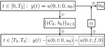
Figure 1: Block diagram of identifiability analysis

3 Numerical computation method

It is seen clearly from previous section that the key point for identification purposes is to recover the spectrum-coefficient data $\left\{(C_{n},\lambda_{n})\right\}_{n\in{\mathbb{N}}_{0}}$ from $\{y(t)|\;t\in[T_{1},T_{2}]\}$ by the Dirichlet series representation:

$$y(t)=\sum_{n=0}^{\infty}C_{n}e^{-\lambda_{n}t},\;t\in[T_{1},T_{2}].$$ (3.1)

The difficulty is that there may exist infinitely many $C_{n}\neq 0$ in (3.1). In this section, we use the matrix pencil method to extract some of the $\{(C_{n},\lambda_{n})\}$ from the sum of the first $M$ terms of the infinite series (3.1), and treat the remainder terms just as a measurement error.

3.1 Finite dimensional approximation of spectral estimation

Suppose $M\in{\mathbb{N}}$ and split the series in (3.1) into two parts:

$$y(t)=\sum_{n=0}^{M-1}C_{n}e^{-\lambda_{n}t}+\sum_{n=M}^{\infty}C_{n}e^{-\lambda_{n}t},\;\forall\;t\in[T_{1},T_{2}].$$ (3.2)

Denote the second series in (3.2) as

$$e(M,t)=\sum_{n=M}^{\infty}C_{n}e^{-\lambda_{n}t},\;\forall\;t\in[T_{1},T_{2}].$$ (3.3)

Theorem 3.1 gives a bound of $e(M,t)$.

Theorem 3.1.

Suppose that the coefficient $\alpha\geq\alpha_{0}>0$ and the initial value $u_{0}(x)$ satisfies

$$\left\|u_{0}\right\|_{L^{2}(0,1)}\leq M_{0}$$ (3.4)

for some $M_{0}>0$. Then for $t\in[T_{1},T_{2}]$,

$$|e(M,t)|<\left(\sqrt{2}+\displaystyle\frac{1}{4M\pi^{2}\alpha_{0}T_{1}}\right)M_{0}e^{-\alpha_{0}M^{2}\pi^{2}T_{1}}.$$ (3.5)

Proof.

According to (2.2) and (3.4),

$$\sum_{n=0}^{\infty}|C_{n}|^{2}\leq 2\|u_{0}\|^{2}\leq 2M_{0}^{2}.$$

Introduce

$$F(\alpha,M,t)=\int_{M}^{\infty}e^{-\alpha x^{2}\pi^{2}t}\;dx,$$ (3.6)

and three regions in $(x,\,y)$ plane:

$$D=\left\{(x,y)\,\bigg{|}\,x\geq M,\;y\geq M\right\},\;D_{1}=\left\{(x,y)\,\bigg{|}\,x\geq y\geq M\right\},\;D_{2}=\left\{(x,y)\,\bigg{|}\,y>x\geq M\right\}.$$

It is obvious that $D=D_{1}\cup D_{2}$ and $D_{1}\cap D_{2}=\emptyset$, and

$$\begin{array}[]{ll}F^{2}(\alpha,M,t)&=\displaystyle\int_{M}^{\infty}e^{-\alpha x^{2}\pi^{2}t}\;dx\cdot\int_{M}^{\infty}e^{-\alpha y^{2}\pi^{2}t}\;dy=\displaystyle\iint_{D}e^{-\alpha(x^{2}+y^{2})\pi^{2}t}\;dxdy\cr\vskip 5.69054pt\cr&=\displaystyle\iint_{D_{1}}e^{-\alpha(x^{2}+y^{2})\pi^{2}t}\;dxdy+\iint\limits_{D_{2}}e^{-\alpha(x^{2}+y^{2})\pi^{2}t}\;dxdy\cr\vskip 5.69054pt\cr&\displaystyle\triangleq I_{1}+I_{2}.\end{array}$$

By symmetry of the integration domains $D_{1}$ and $D_{2}$ with respect to $x$ and $y$, $I_{1}=I_{2}$. To compute $I_{1}$, we use a double integral in polar coordinates to convert it to iterated integrals. The region $D_{1}$ under polar coordinates becomes $\widetilde{D}_{1}$:

$$\widetilde{D}_{1}=\left\{(\rho,\theta)\,\bigg{|}\,\rho\geq\displaystyle\frac{M}{\sin\theta},\;0<\theta\leq\displaystyle\frac{\pi}{4}\right\}.$$

Then we can rewrite the double integral $I_{1}$ as an iterated integral in polar coordinates:

$$\begin{array}[]{ll}I_{1}&=\displaystyle\iint_{D_{1}}e^{-\alpha(x^{2}+y^{2})\pi^{2}t}\;dxdy=\iint\limits_{\widetilde{D}_{1}}e^{-\alpha\rho^{2}\pi^{2}t}\rho\;d\rho d\theta\cr\vskip 5.69054pt\cr&=\displaystyle\int_{0}^{\frac{\pi}{4}}\;d\theta\int_{\frac{M}{\sin\theta}}^{\infty}e^{-\alpha\rho^{2}\pi^{2}t}\rho\;d\rho=\displaystyle\frac{1}{2\alpha\pi^{2}t}\int_{0}^{\frac{\pi}{4}}e^{-\frac{\alpha M^{2}\pi^{2}t}{\sin^{2}\theta}}\;d\theta.\end{array}$$ (3.7)

The variable substitution $u=\cot^{2}\theta$ in (3.7) yields

$$I_{1} = \displaystyle\frac{1}{4\alpha\pi^{2}t}\int_{1}^{+\infty}e^{-\alpha M^{2}\pi^{2}t(1+u)}\displaystyle\frac{1}{(1+u)\sqrt{u}}\;du$$ (3.8)

$$< \displaystyle\frac{1}{4\alpha\pi^{2}t}e^{-\alpha M^{2}\pi^{2}t}\int_{1}^{+\infty}e^{-\alpha M^{2}\pi^{2}tu}u^{-\frac{3}{2}}\;du$$

$$= \displaystyle\frac{M}{4\pi\sqrt{\alpha t}}e^{-\alpha M^{2}\pi^{2}t}\cdot\Gamma\left(-\frac{1}{2},\;\alpha M^{2}\pi^{2}t\right),$$

where

$$\Gamma(a,x)=\int_{x}^{\infty}t^{a-1}e^{-t}\;dt,$$ (3.9)

is the upper incomplete gamma function ([1, Section 6.5]). It is known that [1, p.263]

$$\Gamma(a,x)=e^{-x}x^{a}\left(\displaystyle\frac{1}{x+}\displaystyle\frac{1-a}{1+}\displaystyle\frac{1}{x+}\displaystyle\frac{2-a}{1+}\displaystyle\frac{2}{x+}\cdots\right),\;x>0,\;|a|<\infty,$$ (3.10)

from which we have

$$\Gamma(a,x)<e^{-x}x^{a-1},\;x>0,\;a<0.$$ (3.11)

This together with (3.8) gives

$$I_{1}<\displaystyle\frac{1}{4M^{2}\pi^{4}\alpha^{2}t^{2}}e^{-2\alpha M^{2}\pi^{2}t}.$$ (3.12)

Therefore,

$$F(\alpha,M,t)=\sqrt{2I_{1}}<\displaystyle\frac{1}{\sqrt{2}M\pi^{2}\alpha t}e^{-\alpha M^{2}\pi^{2}t}.$$ (3.13)

We now turn to the estimation of $|e(M,t)|$. It is computed that

$$\begin{array}[]{ll}|e(M,t)|&\leq\displaystyle\sum_{n=M}^{\infty}|C_{n}|e^{-\alpha n^{2}\pi^{2}t}\leq\left(\displaystyle\sum_{n=M}^{\infty}|C_{n}|^{2}\right)^{\frac{1}{2}}\left(\displaystyle\sum_{n=M}^{\infty}e^{-2\alpha n^{2}\pi^{2}t}\right)^{\frac{1}{2}}\cr\vskip 5.69054pt\cr&<\displaystyle\sqrt{2}M_{0}\left[e^{-2\alpha M^{2}\pi^{2}t}+\sum_{n=M+1}^{\infty}\int_{n-1}^{n}e^{-2\alpha x^{2}\pi^{2}t}\;dx\right]^{\frac{1}{2}}\cr\vskip 5.69054pt\cr&=\sqrt{2}M_{0}\cdot\left[e^{-2\alpha M^{2}\pi^{2}t}+F(2\alpha,M,t)\right]^{\frac{1}{2}}\cr\vskip 5.69054pt\cr&<\displaystyle\left(\sqrt{2}+\displaystyle\frac{1}{4M\pi^{2}\alpha t}\right)M_{0}e^{-\alpha M^{2}\pi^{2}t}.\end{array}$$

Since $\alpha\geq\alpha_{0}$, we finally obtain

$$|e(M,t)|<\left(\sqrt{2}+\displaystyle\frac{1}{4M\pi^{2}\alpha_{0}T_{1}}\right)M_{0}e^{-\alpha_{0}M^{2}\pi^{2}T_{1}},\;\forall\;t\in[T_{1},T_{2}].$$ (3.14)

This completes the proof of the theorem. ∎

Remark 3.1.

It is seen from (3.5) that if $\alpha_{0}M^{2}\pi^{2}T_{1}$ is sufficiently large, then it indeed has

$$y(t)\approx\sum_{n=0}^{M-1}C_{n}e^{-\lambda_{n}t},\;\forall\;t\in[T_{1},T_{2}],$$ (3.15)

with the truncation error $e(M,t)$ estimation (3.5).

3.2 Matrix pencil method

The matrix pencil method was first presented by Hua and Sarkar in [11, 12] for estimating signal parameters from a noisy exponential sequence. This method has been proved to be quite useful because of its computational efficiency and low sensitivity to the noise.

Suppose that the observed system response can be described by

$$y(t)=x(t)+n(t)=\displaystyle\sum_{i=1}^{M}R_{i}\exp(s_{i}t)+n(t),\;\forall\;t\in[0,T].$$ (3.16)

where $n(t)$ is the noise, $x(t)$ is the system response, $y(t)$ is the noise contaminated observation, $M$ is the number of exponential components, and $T$ is the maximal observation coverage time.

Let $T_{s}$ be the sampling period. The discrete form of (3.16) can be expressed as follows:

$$y(kT_{s})=x(kT_{s})+n(kT_{s})=\displaystyle\sum_{i=1}^{M}R_{i}z_{i}^{k}+n(kT_{s}),\;k=0,1,\dots,N-1,$$ (3.17)

where $z_{i}=\exp(s_{i}T_{s})$ are the poles of response signal, and $N$ is the number of sample points which should be large enough. Generally, all the number of exponential components $M$, the amplitudes $R_{i}$, and the poles $z_{i}$ can be unknown. In what follows, we show how to estimate these numbers simultaneously from the observation $\left\{y(kT_{s})\right\}_{k=0}^{N-1}$ by virtue of the matrix pencil method.

Let $x_{k}=x(kT_{s})$ and $y_{k}=y(kT_{s})$, and define

$${\bf{x}_{t}}=[x_{t},x_{t+1},\dots,x_{N-L+t-1}]^{\top},\;{\bf{y}_{t}}=[y_{t},y_{t+1},\dots,y_{N-L+t-1}]^{\top},\;t=0,1,2,\dots,L$$ (3.18)

and

$$\begin{array}[]{l}\displaystyle X_{0}=[{\bf{x}_{L-1}},{\bf{x}_{L-2}},\dots,{\bf{x}_{0}}],\;\;Y_{0}=[{\bf{y}_{L-1}},{\bf{y}_{L-2}},\dots,{\bf{y}_{0}}],\cr\vskip 5.69054pt\cr\displaystyle X_{1}=[{\bf{x}_{L}},{\bf{x}_{L-1}},\dots,{\bf{x}_{1}}],\;\;Y_{1}=[{\bf{y}_{L}},{\bf{y}_{L-1}},\dots,{\bf{y}_{1}}],\cr\vskip 5.69054pt\cr\displaystyle X=[{\bf{x}_{0}},{\bf{x}_{1}},\dots,{\bf{x}_{L}}],\;\;Y=[{\bf{y}_{0}},{\bf{y}_{1}},\dots,{\bf{y}_{L}}],\end{array}$$ (3.19)

where the superscript “$\top$” denotes the transpose, and $L$ is called the pencil parameter. It has been pointed out that the best choices for $L$ are $N/3$ and $2N/3$, and all values satisfying $N/3\leq L\leq 2N/3$ appear to be good choices in general [13]. In this paper, the pencil parameter $L$ is always chosen to be $N/3$ or $\lfloor N/3\rfloor+1$ when $N/3$ is not an integer. Here and in the sequel, $\lfloor\cdot\rfloor$ is as usual the floor function and $\lfloor x\rfloor$ denotes the integer part of the number $x$.

Suppose that the singular value decomposition (SVD) of $Y$ is $Y=U\Sigma V^{\top},$ where $U$ and $V$ are $(N-L)\times(N-L)$ and $(L+1)\times(L+1)$ orthogonal matrices, respectively, $\Sigma$ is an $(N-L)\times(L+1)$ diagonal matrix with entries $\{\sigma_{i}\}$ in main diagonal to be the singular values of $Y$.

3.2.1 The estimation of $M$

In case of noiseless observation, i.e. $n(kT_{s})=0$ in (3.17), $M$ is equal to the number of nonzero singular values of the matrix $X$ defined in (3.19), or equivalently the rank of $X$, that is, $M=\operatorname{rank}(X).$

In case of the noise contaminated observation, however, the elements that are originally zeros in main diagonal of $\Sigma$ might not be zeros anymore due to influence of noise. Nevertheless, the values of these elements will be very small as long as the noise is very weak in comparison to the signal (see, e.g., [20]). Thus, an effective practical method for estimating the number $M$ is first to choose the maximal singular value $\sigma_{max}$ of $Y$ and assign a threshold $\varepsilon$ for the singular values, e.g., $\varepsilon=10^{-10}$, and then treat any small singular value $\sigma_{i}$ which satisfies $\sigma_{i}/\sigma_{max}<\varepsilon$ to be zero. Therefore, $M$ can be estimated by

$$M=\#\bigg{\{}\sigma_{i}\Big{|}\;\sigma_{i}\;\mbox{is the singular value of}\;Y\;\mbox{which satisfies}\;\displaystyle\frac{\sigma_{i}}{\sigma_{max}}\geq\varepsilon\bigg{\}}.$$ (3.20)

where $\#S$, here and in the sequel, denotes the number of elements in the set $S$.

3.2.2 Estimation of poles $\left\{z_{i}\right\}_{i=1}^{M}$

In case of noiseless observation, it has been proved in [13, Theorem 2.1] that the poles $\left\{z_{i}\right\}_{i=1}^{M}$ in (3.17) are the $M$ eigenvalues of the matrix $X_{0}^{\dagger}X_{1}$ when $M\leq L\leq N-M$, here and in the sequel the superscript “†” denotes the Moore-Penrose inverse or pseudoinverse. Since $X_{0}^{\dagger}X_{1}$ has rank $M\leq L$, there are also $L-M$ zero eigenvalues for the matrix product.

In case of the noise contaminated observation, suppose that the SVD of $Y_{0}$ is $Y_{0}=U_{0}\Sigma_{0}V_{0}^{\top}$, and the rank-$M$ truncated pseudoinverse $Y_{0,M}^{\dagger}$ is defined as

$$Y_{0,M}^{\dagger}=\sum_{i=1}^{M}\displaystyle\frac{1}{\sigma_{i}}v_{i}u_{i}^{\ast}=V_{0,M}A^{-1}U_{0,M}^{*},$$ (3.21)

where $\left\{\sigma_{i}\right\}_{i=1}^{M}$ are the $M$ largest singular values of $Y_{0}$; $v_{i}$’s and $u_{i}$’s are the corresponding singular vectors, and

$$V_{0,M}=\{v_{1},v_{2},\dots,v_{M}\},\;U_{0,M}=\{u_{1},u_{2},\dots,u_{M}\},\;A=\operatorname{diag}\{\sigma_{1},\sigma_{2},\dots,\sigma_{M}\}.$$ (3.22)

The superscript “$*$” in (3.21) denotes the conjugate transpose.

It is shown in [13] that the estimates of the poles $\left\{z_{i}\right\}_{i=1}^{M}$ can be realized by computing the $M$ nonzero eigenvalues of $Y_{0,M}^{\dagger}Y_{1}$, or equivalently, the eigenvalues of the $M\times M$ matrix

$$Z_{E}=A^{-1}U_{0,M}^{\ast}Y_{1}V_{0,M}.$$ (3.23)

Then the $\left\{s_{i}\right\}_{i=1}^{M}$ in (3.16) can be obtained by

$$s_{i}=\displaystyle\frac{\ln z_{i}}{T_{s}},\;i=1,2,\dots,M.$$ (3.24)

Remark 3.2.

It is easily seen that the matrix pencil method contains truncated singular value decomposition (TSVD) (see, e.g., [10]) as a regularization method to estimate $M$ and $\{z_{i}\}_{i=1}^{M}$.

3.2.3 Estimation of amplitudes $\left\{R_{i}\right\}_{i=1}^{M}$

Having estimated the number $M$ of the exponential components, and all the poles $\left\{z_{i}\right\}_{i=1}^{M}$, the amplitudes $R_{i}$ can be estimated by solving the following linear least squares problem

$$\left\{R_{i}\right\}_{i=1}^{M}=\operatorname{argmin}\sum_{k=0}^{N-1}\bigg{[}y_{k}-\sum_{i=1}^{M}R_{i}z_{i}^{k}\bigg{]}^{2}.$$ (3.25)

3.3 Identification algorithm

Suppose that $0<T_{1}<T_{2}<T_{3}$ are three arbitrary positive numbers, and the control function $f(t)$ is chosen as in (2.6) and the corresponding observation data is $\{y(t)=u(0,t;f,u_{0})|\;t\in[T_{1},T_{3}]\}$. In this section, we formulate the identification for the coefficient and initial value in several steps.

Step 1: Estimate several eigenvalues of system operator ${\cal A}$ from the observation without control by the matrix pencil method.

Specifically, let $T_{1}=t_{0}<t_{1}<\cdots<t_{N_{1}}=T_{2}$ be the uniform grids of $[T_{1},T_{2}]$ with the sampling period $T_{s}=\frac{T_{2}-T_{1}}{N_{1}}$, and the measured values at sample points are

$$y_{i}=y(t_{i})=\displaystyle\sum_{n=0}^{\infty}C_{n}e^{-\lambda_{n}t_{i}}=\displaystyle\sum_{k=0}^{K-1}\left(C_{n_{k}}e^{-\lambda_{n_{k}}T_{1}}\right)e^{-(\lambda_{n_{k}}T_{s})i},\;i=0,1,\dots,N_{1}-1,$$ (3.26)

where $K=\#{\mathbb{K}}$ with ${\mathbb{K}}$ being defined by (2.3) and the series $\left\{C_{n_{k}}\right\}_{k=0}^{K-1}$ consists of all the nonzero elements in the series $\left\{C_{n}\right\}_{n\in{\mathbb{N}}_{0}}$ by removing all the zero ones. Then the number $M$ of the estimable eigenvalues and the approximate eigenvalues $\left\{\widetilde{\lambda}_{n_{k}}\right\}_{k=0}^{M-1}$ can be obtained by virtue of the matrix pencil method following the process introduced in sections 3.2.1 and 3.2.2.

Remark 3.3.

As stated in Theorem 2.1, it is unknown whether the initial value $u_{0}(x)$ is orthogonal to some of the eigenvectors $\{\phi_{n}\}_{n\in{\mathbb{N}}_{0}}$. In case that $\langle u_{0},\phi_{n}\rangle=0$ for some $n\in{\mathbb{N}}_{0}$, then $C_{n}=0$ and the observation has nothing to do with the term $C_{n}e^{-\lambda_{n}t_{i}}$. It is noteworthy that the $\left\{\widetilde{\lambda}_{n_{k}}\right\}_{k=0}^{M-1}$ recovered in Step 1 are the approximations of some eigenvalues of system operator ${\cal A}$, but may not be the first $M$ eigenvalues, i.e. the relationships $\widetilde{\lambda}_{n_{k}}\approx\lambda_{k}\;(=\alpha k^{2}\pi^{2})$ are not always true. In fact, it is true only when $n_{k}=k$ or $\langle u_{0},\phi_{k}\rangle\neq 0$ for $k=0,1,\dots,M-1$, which is the case mentioned in [29], where such an initial value is said to be generic and in this case the Steps 3 and 4 below are not necessary anymore. In other words, when $\langle u_{0},\phi_{k}\rangle=0$ for some $k$, we can not always recover $\alpha$ from $\left\{\widetilde{\lambda}_{n_{k}}\right\}$ directly.

Step 2: Estimate the coefficients $\left\{\widetilde{C}_{n_{k}}\right\}_{k=0}^{M-1}$ that are corresponding to $\left\{\widetilde{\lambda}_{n_{k}}\right\}_{k=0}^{M-1}$ from (3.26) by solving the linear least square problem following

$$\left\{\widetilde{C}_{n_{k}}\right\}_{k=0}^{M-1}=\operatorname{argmin}\sum_{i=0}^{N_{1}-1}\left[y_{i}-\sum_{k=0}^{M-1}\widetilde{C}_{n_{k}}e^{-\widetilde{\lambda}_{n_{k}}t_{i}}\right]^{2}.$$ (3.27)

Remark 3.4.

After obtaining $\left\{\left(\widetilde{C}_{n_{k}},\widetilde{\lambda}_{n_{k}}\right)\right\}_{k=0}^{M-1}$, the control free part of the observation $u(0,t;0,u_{0})$ can be estimated as

$$u(0,t;0,u_{0})\approx\sum_{k=0}^{M-1}\widetilde{C}_{n_{k}}e^{-\widetilde{\lambda}_{n_{k}}t},\;t>0.$$ (3.28)

Step 3: Estimate an approximation of $\alpha$ by obtaining the first several eigenvalues of the operator ${\cal A}$ through the observation data $\{y(t)|\;t\in[T_{2},\;T_{3}]\}$ by virtue of the matrix pencil method.

Similar to Step 1, let $T_{2}=t_{0}<t_{1}<\cdots<t_{N_{2}}=T_{3}$ be the uniform grids of $[T_{2},T_{3}]$ with the sampling period $T_{s}^{\prime}=\frac{T_{3}-T_{2}}{N_{2}}$, and the control is chosen to be $f(t)=1$ for $t\in[T_{2},T_{3}]$. Then from (3.28) we obtain

$$\begin{array}[]{ll}y(t_{i})&=\displaystyle u(0,t_{i};0,u_{0})+u(0,t_{i};f,0)\cr\vskip 5.69054pt\cr&=\displaystyle\sum_{n=0}^{\infty}C_{n}e^{-\lambda_{n}t_{i}}-\int_{0}^{t_{i}}G(t_{i}-s,0,0)f(s)ds\cr\vskip 5.69054pt\cr&\displaystyle\approx\sum_{k=0}^{M-1}\widetilde{C}_{n_{k}}e^{-\widetilde{\lambda}_{n_{k}}t_{i}}-\displaystyle\frac{1}{3\alpha}-(t_{i}-T_{2})+\displaystyle\sum_{n=1}^{\infty}\displaystyle\frac{2}{\lambda_{n}}e^{-\lambda_{n}(t_{i}-T_{2})}\cr\vskip 5.69054pt\cr&=\displaystyle\sum_{k=0}^{M-1}\widetilde{C}_{n_{k}}e^{-\widetilde{\lambda}_{n_{k}}t_{i}}-\displaystyle\frac{1}{3\alpha}-T_{s}^{\prime}i+\sum_{n=1}^{\infty}\displaystyle\frac{2}{\lambda_{n}}e^{-\lambda_{n}T_{s}^{\prime}i}.\end{array}$$ (3.29)

Let

$$y_{i}^{\prime}=y(t_{i})-\sum_{k=0}^{M-1}\widetilde{C}_{n_{k}}e^{-\widetilde{\lambda}_{n_{k}}t_{i}}+T_{s}^{\prime}i,\;i=0,1,\dots,N_{2}-1,$$ (3.30)

and

$$C_{0}^{\prime}=-\displaystyle\frac{1}{3\alpha},\;\;\lambda_{0}^{\prime}=0,\;C_{n}^{\prime}=\displaystyle\frac{2}{\lambda_{n}},\;\;\lambda_{n}^{\prime}=\lambda_{n}T_{s}^{\prime},\;n\in{\mathbb{N}}.$$ (3.31)

Then (3.29) becomes

$$y_{i}^{\prime}\approx\sum_{n=0}^{\infty}C_{n}^{\prime}e^{-\lambda_{n}^{\prime}i},\;i=0,1,\dots,N_{2}-1.$$ (3.32)

Next, we estimate $\left\{\left(C_{n}^{\prime},\lambda_{n}^{\prime}\right)\right\}_{n=0}^{M^{\prime}-1}$ from (3.32) by repeating the processes in Steps 1 and 2. Then $\alpha$ can be obtained from (1.3) and (3.31).

Remark 3.5.

The estimation process for $\left\{\left(C_{n}^{\prime},\lambda_{n}^{\prime}\right)\right\}_{n=0}^{M^{\prime}-1}$ from (3.32) is slightly different in Step 1 since none of the $\left\{C_{n}^{\prime}\right\}_{n=0}^{M^{\prime}-1}$ is zero although they are also unknown. Hence, we can recover $\alpha$ from one of the following relations:

$$\lambda_{n}^{\prime}=\alpha n^{2}\pi^{2}T_{s}^{\prime},\;n=1,2,\dots,M^{\prime}-1,$$ (3.33)

and

$$C_{n}^{\prime}=\displaystyle\frac{2}{\alpha n^{2}\pi^{2}},\;n=1,2,\dots,M^{\prime}-1.$$ (3.34)

However, the $\alpha$ obtained from (3.33) may be different from that obtained from (3.34) since both $\left\{C_{n}^{\prime}\right\}$ and $\left\{\lambda_{n}^{\prime}\right\}$ are estimated values rather than exact ones. In simulations, the pairs $(C_{n}^{\prime},\lambda_{n}^{\prime})$ that satisfy

$$C_{n}^{\prime}\lambda_{n}^{\prime}\approx 2T_{s}^{\prime},\;n=1,2,\dots,M^{\prime}-1.$$ (3.35)

seem to be more credible to estimate $\alpha$. Actually, the estimated coefficient here is only for identification $\left\{n_{k}\right\}_{k=0}^{M-1}$ from $\left\{\widetilde{\lambda}_{n_{k}}\right\}_{k=0}^{M-1}$ which is shown in succeeding Step 4. Finally, we emphasize that the identification of $\alpha$ does not depend on the sampling period but the special structure of eigenvalues (3.33). If there is no such structure for eigenvalues, our idea of transforming the identification of $\alpha$ to be a zero initial value problem can simplify the problem.

Step 4: Estimate $\alpha$ from $\left\{\widetilde{\lambda}_{n_{k}}\right\}_{k=0}^{M-1}$ and reconstruct the initial state $u_{0}(x)$.

To be specific, after estimating $\left\{\left(\widetilde{C}_{n_{k}},\widetilde{\lambda}_{n_{k}}\right)\right\}_{k=0}^{M-1}$ in Steps 1, 2, and recovering an approximation of $\alpha$ in Step 3, we can now determine the series ${\mathbb{K}}_{M}=\left\{n_{k}\right\}_{k=0}^{M-1}$ by

$$n_{k}=\left\lfloor\sqrt{\displaystyle\frac{\widetilde{\lambda}_{n_{k}}}{\alpha\pi^{2}}}\;\right\rceil,\;k=0,1,\dots,M-1,$$ (3.36)

where $\lfloor x\rceil$ denotes the integer nearest to $x$. Then, $\alpha$ can be estimated by

$$\alpha_{k}=\displaystyle\frac{\widetilde{\lambda}_{n_{k}}}{n_{k}^{2}\pi^{2}}\mbox{ for }n_{k}\neq 0,\;k=0,1,\dots,M-1.$$ (3.37)

An error analysis between the estimated coefficient $\alpha_{k}$ and the real value is discussed in section 5.

Now we turn to initial value. It is clear from (1.7) that

$$y(t)=\displaystyle\sum_{n=0}^{\infty}A_{n}(0)e^{-\lambda_{n}t}=\displaystyle\sum_{n=0}^{\widetilde{M}-1}A_{n}(0)e^{-\alpha n^{2}\pi^{2}t}+e(\widetilde{M},t),\;\forall\;t\in[T_{0},T_{2}),$$ (3.38)

where $T_{0}\in(0,T_{2})$. It follows from Theorem 3.1 that we can choose proper $\widetilde{M}$ and $T_{0}$ such that $\left|e(\widetilde{M},t)\right|$ is sufficiently small. Suppose that only observation at the sample points $T_{0}=t_{0}<t_{1}<\dots<t_{N}=T_{2}$ are available. Then the coefficients $\left\{A_{n}(0)\right\}$ can be estimated by solving the following problem properly

$$\sum_{i=0}^{N-1}\left[y(t_{i})-\sum_{n=0}^{\widetilde{M}-1}A_{n}(0)e^{-\alpha n^{2}\pi^{2}t_{i}}\right]^{2},$$ (3.39)

or equivalently, finding the least squares solution of the matrix equation

$$CA=b,$$ (3.40)

where $C$ is an $N\times\widetilde{M}$ matrix with the $(i,j)$ element

$$C(i,j)=e^{-\alpha(j-1)^{2}\pi^{2}t_{i-1}},$$ (3.41)

and

$$A=[A_{0}(0),A_{1}(0),\cdots,A_{\widetilde{M}-1}(0)]^{\top},\;b=[y(t_{0}),y(t_{1}),\cdots,y(t_{N-1})]^{\top}.$$ (3.42)

Since the reconstruction of the initial value is known to be ill-posed, which results in the resulting matrix equation (3.40) to be ill-posed as well. In order to obtain stable results, some regularization method is required. Here we use the TSVD [10] to solve the matrix equation (3.40).

Suppose that the SVD of matrix $C$ is

$$C=U_{C}\Sigma_{C}V_{C}^{\top},$$ (3.43)

where $U_{C}=[u_{1}^{\prime},u_{2}^{\prime},\cdots,u_{N}^{\prime}]$ and $V_{C}=[v_{1}^{\prime},v_{2}^{\prime},\cdots,v_{\widetilde{M}}^{\prime}]$ are orthonormal matrices with column vectors named left and right singular vectors, respectively. $\Sigma_{C}=\operatorname{diag}(\sigma_{1},\sigma_{2},\cdots)$ is a diagonal matrix with non-negative diagonal elements being the singular values of $C$. In the TSVD method, the matrix $C$ is replaced by its rank-$k$ approximation, and the regularized solution is given by

$$A_{reg}=\sum_{i=1}^{k}\displaystyle\frac{u_{i}^{\prime\top}b}{\sigma_{i}}v_{i}^{\prime}.$$ (3.44)

where $k\leq\operatorname{rank}(C)$ is the regularization parameter. In this paper, we use the generalized cross-validation (GCV) criterion [7] to determine the regularization parameter. The GCV criterion determines the optimal regularization parameter $k$ by minimizing the following GCV function:

$$G(k)=\displaystyle\frac{\|CA_{reg}-b\|^{2}}{(trace(I_{N}-CC^{I}))^{2}},$$ (3.45)

where $C^{I}$ is the matrix which produces the regularized solution after being multiplied with the right-hand side $b$, i.e. $A_{reg}=C^{I}b$.

Having obtained the regularized solution $A_{reg}$, then the initial value can be estimated by the asymptotic Fourier series expansion:

$$u_{0}(x)\approx\sum_{n=0}^{\widetilde{M}-1}A_{n}(0)\cos n\pi x.$$ (3.46)

Remark 3.6.

It is obvious that the reconstructed initial value $\widetilde{u}_{0}(x)$ by (3.46) is an approximated Fourier series expansion of $u_{0}(x)$ with the first $\widetilde{M}$ terms. In fact, since $\alpha$ has been estimated, there are various methods for the initial state reconstruction, see, e.g., [26, 34] and the references therein. Compared with those methods, the method here is more direct and simple.

4 Error analysis

Noise sensitivity of the matrix pencil method for estimating finite signal parameters from a noisy exponential sequence is analyzed in [13]. But our case is different in two aspects. First, the number of unknown parameters in the infinite spectral estimation is not finite. Second, the perturbation, that is, the remainder term $e(M,t)$ in (3.3), is not random. In this section, we establish an error analysis by applying the matrix pencil method to the infinite spectral estimation problem:

$$y(t)=\sum_{n=0}^{\infty}C_{n}e^{-\lambda_{n}t},\;\forall\;t\in[T_{1},T_{2}].$$ (4.1)

We may suppose without loss of generality that $C_{n}\neq 0$ for any $n\in{\mathbb{N}}_{0}$. In fact, we are only concerned with the first $M$ nonzero terms in series (4.1) which is written in a clear way as

$$y(t)=x(t)+e(M,t)=\sum_{n=0}^{M-1}C_{n}e^{-\lambda_{n}t}+\sum_{n=M}^{\infty}C_{n}e^{-\lambda_{n}t},\;\forall\;t\in[T_{1},T_{2}],$$ (4.2)

where $M$ is defined as (3.20). Let $T_{1}=t_{0}<t_{1}<\cdots<t_{N-1}=T_{2}$ be the points on a uniform grid of $[T_{1},T_{2}]$ with the sampling period $T_{s}=\frac{T_{2}-T_{1}}{N-1}$, and hence the observation data at sample points, $t_{i}$, are

$$\begin{array}[]{ll}y_{i}=y(t_{i})&=\displaystyle\sum_{n=0}^{\infty}\left(C_{n}e^{-\lambda_{n}T_{1}}\right)e^{-(\lambda_{n}T_{s})i}=\sum_{n=0}^{M-1}\left(C_{n}e^{-\lambda_{n}T_{1}}\right)e^{-(\lambda_{n}T_{s})i}+e(M,t_{i})\cr\vskip 5.69054pt\cr&\displaystyle\triangleq\sum_{n=0}^{M-1}\left(C_{n}e^{-\lambda_{n}T_{1}}\right)z_{n}^{i}+e(M,t_{i}),\end{array}$$ (4.3)

where $z_{n}=e^{-\lambda_{n}T_{s}}$. By Theorem 3.1, it follows that

$$\begin{array}[]{ll}|y_{i}-x_{i}|=|e(M,t_{i})|&\displaystyle<\left(\sqrt{2}+\displaystyle\frac{1}{4M\pi^{2}\alpha_{0}t_{i}}\right)M_{0}e^{-\alpha M^{2}\pi^{2}t_{i}}\cr\vskip 5.69054pt\cr&\displaystyle\leq\left(\sqrt{2}+\displaystyle\frac{1}{4M\pi^{2}\alpha_{0}T_{1}}\right)M_{0}e^{-\alpha_{0}M^{2}\pi^{2}T_{1}}e^{-\alpha_{0}M^{2}\pi^{2}T_{s}i},\end{array}$$ (4.4)

where $x_{i}=\sum_{n=0}^{M-1}\left(C_{n}e^{-\lambda_{n}T_{1}}\right)z_{n}^{i}$. Define the matrices $X_{0},\;Y_{0},\;X_{1},\;Y_{1}$ as (3.18)-(3.19). Theorem 4.1 below gives the bounds of $\|Y_{0}-X_{0}\|_{F}$ and $\|Y_{1}-X_{1}\|_{F}$, where $\|\cdot\|_{F}$ denotes the matrix Frobenius norm.

Theorem 4.1.

Let the number of sample points $N>9$ and

$$\theta=2\alpha_{0}M^{2}\pi^{2}T_{s}.$$ (4.5)

Then

$$\|Y_{0}-X_{0}\|_{F}<\left(\sqrt{2}+\displaystyle\frac{1}{4M\pi^{2}\alpha_{0}T_{1}}\right)M_{0}e^{-\alpha_{0}M^{2}\pi^{2}T_{1}}\sqrt{M_{\theta,L}+\left(1+\displaystyle\frac{1}{\theta}\right)^{2}},$$ (4.6)

and

$$\|Y_{1}-X_{1}\|_{F}<\left(\sqrt{2}+\displaystyle\frac{1}{4M\pi^{2}\alpha_{0}T_{1}}\right)M_{0}e^{-\alpha_{0}M^{2}\pi^{2}T_{1}}\sqrt{M_{\theta,L+1}+\displaystyle\frac{1}{\theta}\left(1+\displaystyle\frac{1}{\theta}\right)e^{-\theta}},$$ (4.7)

where

$$M_{\theta,L}=\left\{\begin{array}[]{ll}e^{-\theta},&\theta\geq 1,\\ \displaystyle\frac{2}{\theta}e^{-1},&\displaystyle\frac{1}{L-1}<\theta<1,\\ (L-1)e^{-(L-1)\theta},&0<\theta\leq\displaystyle\frac{1}{L-1},\end{array}\right.$$ (4.8)

Proof.

Since both matrices $X_{0}$ and $Y_{0}$ admit the Hankel structure, it is easy to deduce from the definition of Frobenius norm that

$$\begin{array}[]{ll}\|Y_{0}-X_{0}\|_{F}^{2}&=\displaystyle\sum_{i=0}^{L-1}(i+1)\left|y_{i}-x_{i}\right|^{2}+\sum_{i=1}^{L}i\left|y_{N-1-i}-x_{N-1-i}\right|^{2}+L\sum_{i=L}^{N-L-2}\left|y_{i}-x_{i}\right|^{2}\cr\vskip 5.69054pt\cr&\leq\displaystyle\left(\sqrt{2}+\displaystyle\frac{1}{4M\pi^{2}\alpha_{0}T_{1}}\right)^{2}M_{0}^{2}e^{-2\alpha_{0}M^{2}\pi^{2}T_{1}}\bigg{[}\sum_{i=0}^{L-1}ie^{-\theta i}+\sum_{i=0}^{L-1}e^{-\theta i}\cr\vskip 5.69054pt\cr&\hskip 8.5359pt+\displaystyle\sum_{i=1}^{L}ie^{-\theta(N-1-i)}+L\sum_{i=L}^{N-L-2}e^{-\theta i}\bigg{]}\cr\vskip 5.69054pt\cr&\displaystyle\triangleq\left(\sqrt{2}+\displaystyle\frac{1}{4M\pi^{2}\alpha_{0}T_{1}}\right)^{2}M_{0}^{2}e^{-2\alpha_{0}M^{2}\pi^{2}T_{1}}\left[S_{1}+S_{2}+S_{3}+S_{4}\right].\end{array}$$

To estimate $S_{1}$, we introduce

$$f(x)=xe^{-\theta x},\;x\geq 0,$$ (4.9)

which satisfies

$$f^{\prime}(x)=(1-\theta x)e^{-\theta x},\;x\geq 0.$$

There are three different cases according to the values of $\theta$.

Case 1: $\theta\geq 1$. In this case, $f^{\prime}(x)\leq 0$ for $x\geq 1$. Hence

$$ie^{-\theta i}\leq\int_{i-1}^{i}xe^{-\theta x}dx,\;i=2,3,\dots,L-1.$$ (4.10)

Therefore,

$$S_{1}=e^{-\theta}+\sum_{i=2}^{L-1}ie^{-\theta i}\leq e^{-\theta}+\sum_{i=2}^{L-1}\int_{i-1}^{i}xe^{-\theta x}dx=e^{-\theta}+\int_{1}^{L-1}xe^{-\theta x}dx.$$

Case 2: $\frac{1}{L-1}<\theta<1$. In this case, $f^{\prime}(x)\geq 0$ for $0\leq x\leq\displaystyle\frac{1}{\theta}$, and $f^{\prime}(x)<0$ for $x>\displaystyle\frac{1}{\theta}$, which imply

$$f(x)\leq f({\theta}^{-1})=\displaystyle\frac{1}{\theta}e^{-1},\;x\geq 0,$$

and

$$ie^{-\theta i}\leq\int_{i}^{i+1}xe^{-\theta x}dx,\;i=1,\dots,\left\lfloor\displaystyle\frac{1}{\theta}\right\rfloor-1.$$ (4.11)

$$ie^{-\theta i}\leq\int_{i-1}^{i}xe^{-\theta x}dx,\;i=\left\lfloor\displaystyle\frac{1}{\theta}\right\rfloor+2,\dots,L-1.$$ (4.12)

Thus

$$S_{1} = \sum_{i=1}^{L-1}ie^{-\theta i}=\sum_{i=1}^{\lfloor\frac{1}{\theta}\rfloor-1}ie^{-\theta i}+\left\lfloor\displaystyle\frac{1}{\theta}\right\rfloor e^{-\theta\lfloor\frac{1}{\theta}\rfloor}+\left(\left\lfloor\displaystyle\frac{1}{\theta}\right\rfloor+1\right)e^{-\theta(\lfloor\frac{1}{\theta}\rfloor+1)}+\sum_{i=\lfloor\frac{1}{\theta}\rfloor+2}^{L-1}ie^{-\theta i}$$

$$\leq \sum_{i=1}^{\lfloor\frac{1}{\theta}\rfloor-1}\int_{i}^{i+1}xe^{-\theta x}dx+f\left(\left\lfloor\displaystyle\frac{1}{\theta}\right\rfloor\right)+f\left(\left\lfloor\displaystyle\frac{1}{\theta}\right\rfloor+1\right)+\sum_{i=\lfloor\frac{1}{\theta}\rfloor+2}^{L-1}\int_{i-1}^{i}xe^{-\theta x}dx$$

$$\leq \int_{1}^{\lfloor\frac{1}{\theta}\rfloor}xe^{-\theta x}dx+2f\left(\displaystyle\frac{1}{\theta}\right)+\int_{\lfloor\frac{1}{\theta}\rfloor+1}^{L-1}xe^{-\theta x}dx$$

$$\leq \displaystyle\frac{2}{\theta}e^{-1}+\int_{1}^{L-1}xe^{-\theta x}dx.$$

Case 3: $0<\theta\leq\displaystyle\frac{1}{L-1}$. In this case, $f^{\prime}(x)\geq 0$ for $0\leq x\leq L-1$. Hence

$$ie^{-\theta i}\leq\int_{i}^{i+1}xe^{-\theta x}dx,\;i=1,\dots,L-2.$$ (4.13)

Therefore,

$$S_{1} = \sum_{i=1}^{L-2}ie^{-\theta i}+(L-1)e^{-(L-1)\theta}\leq(L-1)e^{-(L-1)\theta}+\sum_{i=1}^{L-2}\int_{i}^{i+1}xe^{-\theta x}dx$$

$$= (L-1)e^{-(L-1)\theta}+\int_{1}^{L-1}xe^{-\theta x}dx$$

Combining the three cases discussed above gives

$$S_{1}\leq M_{\theta,L}+\int_{1}^{L-1}xe^{-\theta x}dx=M_{\theta,L}+\displaystyle\frac{1}{\theta}\left(1+\displaystyle\frac{1}{\theta}\right)e^{-\theta}-\displaystyle\frac{1}{\theta}\left(L-1+\displaystyle\frac{1}{\theta}\right)e^{-\theta(L-1)},$$ (4.14)

where $M_{\theta,L}$ is defined in (4.8).

An analogous but simpler analysis of $S_{2},\;S_{3}$, and $S_{4}$ gives

$$S_{2}\leq 1+\displaystyle\frac{1}{\theta}-\displaystyle\frac{1}{\theta}e^{-\theta(L-1)},$$

$$S_{3}\leq\displaystyle\frac{1}{\theta}e^{-\theta(N-2)}\left[\left(L+1-\displaystyle\frac{1}{\theta}\right)e^{\theta L}+\displaystyle\frac{1}{\theta}-1\right]\triangleq M_{\theta,N},$$ (4.15)

$$S_{4}\leq\displaystyle\frac{L}{\theta}\left[e^{-\theta(L-1)}-e^{-\theta(N-L-2)}\right].$$

We next show when $N>9$,

$$M_{\theta,N}<\displaystyle\frac{1}{\theta^{2}}e^{-\theta(L-1)}+\displaystyle\frac{L}{\theta}e^{-\theta(N-L-2)}.$$ (4.16)

Since $L=N/3$ or $L=\lfloor N/3\rfloor+1$ if $N/3$ is not an integer, it follows that $L\geq 4$ when $N>9$, hence

$$\begin{array}[]{ll}M_{\theta,N}-\displaystyle\frac{1}{\theta^{2}}e^{-\theta(L-1)}-\displaystyle\frac{L}{\theta}e^{-\theta(N-L-2)}&=\displaystyle\displaystyle\frac{1}{\theta^{2}}e^{-\theta(N-2)}\left[(\theta-1)\left(e^{\theta L}-1\right)-e^{\theta(N-L-1)}\right]\cr\vskip 5.69054pt\cr&\leq\displaystyle\displaystyle\frac{1}{\theta^{2}}e^{-\theta(N-2)}\left[(\theta-1)\left(e^{\theta L}-1\right)-e^{\theta(2L-3)}\right]\cr\vskip 5.69054pt\cr&<\displaystyle\displaystyle\frac{1}{\theta^{2}}e^{-\theta(N-2)}\left(e^{\theta L}-1\right)\left[\theta-e^{(L-3)\theta}\right]\cr\vskip 5.69054pt\cr&<0.\end{array}$$ (4.17)

As a consequence,

$$S_{1}+S_{2}+S_{3}+S_{4} \leq M_{\theta,L}+\displaystyle\frac{1}{\theta}\left(1+\displaystyle\frac{1}{\theta}\right)e^{-\theta}-\displaystyle\frac{1}{\theta}\left(L-1+\displaystyle\frac{1}{\theta}\right)e^{-\theta(L-1)}+1+\displaystyle\frac{1}{\theta}$$

$$-\displaystyle\frac{1}{\theta}e^{-\theta(L-1)}+M_{\theta,N}+\displaystyle\frac{L}{\theta}\left[e^{-\theta(L-1)}-e^{-\theta(N-L-2)}\right]$$

$$= M_{\theta,L}+\displaystyle\frac{1}{\theta}\left(1+\displaystyle\frac{1}{\theta}\right)e^{-\theta}-\displaystyle\frac{1}{\theta^{2}}e^{-\theta(L-1)}+1+\displaystyle\frac{1}{\theta}+M_{\theta,N}-\displaystyle\frac{L}{\theta}e^{-\theta(N-L-2)}$$

$$< M_{\theta,L}+\left(1+\displaystyle\frac{1}{\theta}\right)^{2}.$$

Hence

$$\|Y_{0}-X_{0}\|_{F} < \left(\sqrt{2}+\displaystyle\frac{1}{4M\pi^{2}\alpha_{0}T_{1}}\right)M_{0}e^{-\alpha_{0}M^{2}\pi^{2}T_{1}}\sqrt{S_{1}+S_{2}+S_{3}+S_{4}}$$

$$< \left(\sqrt{2}+\displaystyle\frac{1}{4M\pi^{2}\alpha_{0}T_{1}}\right)M_{0}e^{-\alpha_{0}M^{2}\pi^{2}T_{1}}\sqrt{M_{\theta,L}+\left(1+\displaystyle\frac{1}{\theta}\right)^{2}}.$$

By almost the same analysis to $\|Y_{1}-X_{1}\|_{F}$, we can achieve the estimation (4.7). The details are omitted. This completes the proof of the theorem. ∎

The next lemmas show the effect of perturbations in a matrix to its generalized inverse or eigenvalues.

Lemma 4.1.

([28]) For any two matrices $A$ and $B$ with $B=A+E$, if $\operatorname{rank}(A)=\operatorname{rank}(B)$, then

$$\left\|B^{\dagger}-A^{\dagger}\right\|_{2}\leq\displaystyle\frac{1+\sqrt{5}}{2}\left\|A^{\dagger}\right\|_{2}\cdot\left\|B^{\dagger}\right\|_{2}\cdot\left\|E\right\|_{2},$$ (4.18)

where $\|\cdot\|_{2}$ denotes the matrix spectral norm (matrix 2-norm).

Lemma 4.2.

([33]) If

$$\operatorname{rank}(A+E)=\operatorname{rank}(A)\;\;and\;\;\left\|E\right\|_{2}<\displaystyle\frac{1}{\left\|A^{\dagger}\right\|_{2}},$$ (4.19)

then

$$\left\|(A+E)^{\dagger}\right\|_{2}\leq\displaystyle\frac{\left\|A^{\dagger}\right\|_{2}}{1-\left\|A^{\dagger}\right\|_{2}\cdot\|E\|_{2}}.$$ (4.20)

Lemma 4.3.

([2]) If $A$ is diagonalizable, i.e.,

$$A=X\Lambda X^{-1},\;where\;\Lambda=\operatorname{diag}(\lambda_{1},\dots,\lambda_{n}),$$

then for any $\widetilde{\lambda}\in\lambda(\widetilde{A})$, there exists a $\lambda\in\lambda(A)$ such that

$$|\widetilde{\lambda}-\lambda|\leq\kappa(X)\cdot\left\|\widetilde{A}-A\right\|_{2},$$ (4.21)

where $\lambda(A)$ is the set of the eigenvalues of $A$ and $\kappa(X)$ is the (spectral) condition number of $X$, defined as

$$\kappa(X)=\|X\|_{2}\cdot\left\|X^{-1}\right\|_{2}.$$

Suppose the singular values of $Y_{0}$ are $\sigma(Y_{0})=\{\sigma_{i}\}$ and $Y_{0,M}$ is the rank-$M$ truncated approximation of $Y_{0}$ defined by

$$Y_{0,M}=U_{0,M}AV_{0,M}^{\top},$$ (4.22)

where $U_{0,M},\;A$, and $V_{0,M}$ are defined in (3.22). Now we are in a position to give an error analysis for the infinite spectral estimation problem (4.1) using the matrix pencil method.

Theorem 4.2.

Let $\sigma_{1}\geq\sigma_{2}\geq\dots\geq\sigma_{M}$ be the first $M$ singular values of the matrix $Y_{0}$, and assume that $Y_{0,M}^{\dagger}Y_{1}$ is diagonalizable, i.e. $Y_{0,M}^{\dagger}Y_{1}=X_{M}\widetilde{\Lambda}_{M}X_{M}^{-1},$ where

$$\widetilde{\Lambda}_{M}=\operatorname{diag}(\widetilde{z}_{1},\dots,\widetilde{z}_{M},0,\dots,0),\;\widetilde{z}_{1}\geq\widetilde{z}_{2}\geq\dots\geq\widetilde{z}_{M}.$$

The nonzero eigenvalues of the matrix $X_{0}^{\dagger}X_{1}$ are supposed to be

$$\Lambda_{M}=\{z_{1},z_{2},\dots,z_{M}\},\;z_{1}\geq z_{2}\geq\dots\geq z_{M}.$$

Let $\theta$ and $M_{\theta,L}$ be defined as in (4.5), (4.8), respectively, and let

$$\rho=\left(\left\|Y_{0,M}-Y_{0}\right\|_{2}+\left(\sqrt{2}+\displaystyle\frac{1}{4M\pi^{2}\alpha_{0}T_{1}}\right)M_{0}e^{-\alpha_{0}M^{2}\pi^{2}T_{1}}\sqrt{M_{\theta,L}+\left(1+\displaystyle\frac{1}{\theta}\right)^{2}}\right)\bigg{/}\sigma_{M}.$$ (4.23)

If $\rho<1$, then

$$\begin{array}[]{ll}|\widetilde{z}_{n}-z_{n}|<&\displaystyle\displaystyle\frac{\kappa(X_{M})}{\sigma_{M}\cdot(1-\rho)}\cdot\Bigg{[}\displaystyle\frac{1+\sqrt{5}}{2}\rho\|Y_{1}\|_{2}+\displaystyle\left(\sqrt{2}+\displaystyle\frac{1}{4M\pi^{2}\alpha_{0}T_{1}}\right)M_{0}e^{-\alpha_{0}M^{2}\pi^{2}T_{1}}\cr\vskip 5.69054pt\cr&\times\sqrt{M_{\theta,L+1}+\displaystyle\frac{1}{\theta}\left(1+\displaystyle\frac{1}{\theta}\right)e^{-\theta}}\Bigg{]}.\end{array}$$ (4.24)

In particular, if $\theta>\displaystyle\frac{1}{L-1}$, then

$$|\widetilde{z}_{n}-z_{n}|<\displaystyle\frac{\kappa(X_{M})\cdot\rho}{\sigma_{M}\cdot(1-\rho)}\cdot\left[\displaystyle\frac{1+\sqrt{5}}{2}\|Y_{1}\|_{2}+\sigma_{M}\right].$$ (4.25)

Proof.

We need to estimate the matrix norm $\left\|Y_{0,M}^{\dagger}Y_{1}-X_{0}^{\dagger}X_{1}\right\|_{2}$ first, which is done as follows:

$$\left\|Y_{0,M}^{\dagger}Y_{1}-X_{0}^{\dagger}X_{1}\right\|_{2} = \left\|Y_{0,M}^{\dagger}Y_{1}-X_{0}^{\dagger}Y_{1}+X_{0}^{\dagger}Y_{1}-X_{0}^{\dagger}X_{1}\right\|_{2}$$

$$\leq \left\|Y_{0,M}^{\dagger}Y_{1}-X_{0}^{\dagger}Y_{1}\right\|_{2}+\left\|X_{0}^{\dagger}Y_{1}-X_{0}^{\dagger}X_{1}\right\|_{2}$$

$$\leq \left\|Y_{0,M}^{\dagger}-X_{0}^{\dagger}\right\|_{2}\cdot\|Y_{1}\|_{2}+\left\|X_{0}^{\dagger}\right\|_{2}\cdot\|Y_{1}-X_{1}\|_{2}.$$

Since $Y_{0,M}$ is the rank-$M$ truncated matrix of $Y_{0}$, $\operatorname{rank}(X_{0})=M=\operatorname{rank}(Y_{0,M})$. An application of Lemma 4.1 yields

$$\left\|Y_{0,M}^{\dagger}-X_{0}^{\dagger}\right\|_{2}\leq\displaystyle\frac{1+\sqrt{5}}{2}\left\|Y_{0,M}^{\dagger}\right\|_{2}\cdot\left\|X_{0}^{\dagger}\right\|_{2}\cdot\left\|Y_{0,M}-X_{0}\right\|_{2}.$$ (4.26)

So

$$\left\|Y_{0,M}^{\dagger}Y_{1}-X_{0}^{\dagger}X_{1}\right\|_{2}\leq\displaystyle\frac{1+\sqrt{5}}{2}\left\|Y_{0,M}^{\dagger}\right\|_{2}\cdot\left\|X_{0}^{\dagger}\right\|_{2}\cdot\|Y_{0,M}-X_{0}||_{2}\cdot\|Y_{1}\|_{2}+\left\|X_{0}^{\dagger}\right\|_{2}\cdot\|Y_{1}-X_{1}\|_{2}.$$ (4.27)

Since $\left\|Y_{0,M}^{\dagger}\right\|_{2}=\displaystyle\frac{1}{\sigma_{M}}$,

$$\begin{array}[]{ll}\displaystyle\left\|Y_{0,M}-X_{0}\right\|_{2}\cdot\left\|Y_{0,M}^{\dagger}\right\|_{2}&\leq\displaystyle\left(\left\|Y_{0,M}-Y_{0}\right\|_{2}+\left\|Y_{0}-X_{0}\right\|_{2}\right)\cdot\left\|Y_{0,M}^{\dagger}\right\|_{2}\cr\vskip 5.69054pt\cr&\leq\displaystyle\left(\left\|Y_{0,M}-Y_{0}\right\|_{2}+\left\|Y_{0}-X_{0}\right\|_{F}\right)\cdot\left\|Y_{0,M}^{\dagger}\right\|_{2}\cr\vskip 5.69054pt\cr&<\rho,\end{array}$$

where the last inequality is based on the estimation of $\|Y_{0}-X_{0}\|_{F}$ in Theorem 4.1. Since $\rho<1$, it follows from Lemma 4.2 that

$$\left\|X_{0}^{\dagger}\right\|_{2}\leq\displaystyle\frac{\left\|Y_{0,M}^{\dagger}\right\|_{2}}{1-\left\|Y_{0,M}^{\dagger}\right\|_{2}\cdot\left\|Y_{0,M}-X_{0}\right\|_{2}}<\displaystyle\frac{1}{(1-\rho)\sigma_{M}}.$$ (4.28)

As a result,

$$\left\|Y_{0,M}^{\dagger}Y_{1}-X_{0}^{\dagger}X_{1}\right\|_{2} \leq \left\|X_{0}^{\dagger}\right\|_{2}\cdot\left[\displaystyle\frac{1+\sqrt{5}}{2}\left\|Y_{0,M}^{\dagger}\right\|_{2}\cdot\|Y_{0,M}-X_{0}||_{2}\cdot\|Y_{1}\|_{2}+\|Y_{1}-X_{1}\|_{2}\right]$$

$$< \displaystyle\frac{1}{(1-\rho)\cdot\sigma_{M}}\left[\displaystyle\frac{1+\sqrt{5}}{2}\rho\|Y_{1}\|_{2}+\|Y_{1}-X_{1}||_{F}\right].$$

By Lemma 4.3, we have

$$|\widetilde{z}_{n}-z_{n}| \leq \kappa(X_{M})\cdot\left\|Y_{0,M}^{\dagger}Y_{1}-X_{0}^{\dagger}X_{1}\right\|_{2}<\displaystyle\frac{\kappa(X_{M})}{(1-\rho)\cdot\sigma_{M}}\left[\displaystyle\frac{1+\sqrt{5}}{2}\rho\|Y_{1}\|_{2}+\|Y_{1}-X_{1}||_{F}\right]$$

$$< \displaystyle\frac{\kappa(X_{M})}{\sigma_{M}\cdot(1-\rho)}\cdot\Bigg{[}\displaystyle\frac{1+\sqrt{5}}{2}\rho\|Y_{1}\|_{2}+\left(\sqrt{2}+\displaystyle\frac{1}{4M\pi^{2}\alpha_{0}T_{1}}\right)M_{0}e^{-\alpha_{0}M^{2}\pi^{2}T_{1}}$$

$$\times\sqrt{M_{\theta,L+1}+\displaystyle\frac{1}{\theta}\left(1+\displaystyle\frac{1}{\theta}\right)e^{-\theta}}\Bigg{]}.$$

In particular, if $\theta>\displaystyle\frac{1}{L-1}$, it follows from the definition of $M_{\theta,L}$ in (4.8) that

$$M_{\theta,L+1}=M_{\theta,L},\;\;\theta>\displaystyle\frac{1}{L-1}.$$ (4.29)

On the other hand, since

$$\frac{1}{\theta}\left(1+\displaystyle\frac{1}{\theta}\right)e^{-\theta}<\left(1+\displaystyle\frac{1}{\theta}\right)^{2},\;\;\theta>0,$$

it follows from (4.29) that

$$\sqrt{M_{\theta,L+1}+\displaystyle\frac{1}{\theta}\left(1+\displaystyle\frac{1}{\theta}\right)e^{-\theta}}<\sqrt{M_{\theta,L}+\left(1+\displaystyle\frac{1}{\theta}\right)^{2}},$$

and then

$$|\widetilde{z}_{n}-z_{n}| < \displaystyle\frac{\kappa(X_{M})}{\sigma_{M}\cdot(1-\rho)}\cdot\Bigg{[}\displaystyle\frac{1+\sqrt{5}}{2}\rho\|Y_{1}\|_{2}+\left(\sqrt{2}+\displaystyle\frac{1}{4M\pi^{2}\alpha_{0}T_{1}}\right)M_{0}e^{-\alpha_{0}M^{2}\pi^{2}T_{1}}$$

$$\times\sqrt{M_{\theta,L}+\left(1+\displaystyle\frac{1}{\theta}\right)^{2}}\Bigg{]}$$

$$= \displaystyle\frac{\kappa(X_{M})}{\sigma_{M}\cdot(1-\rho)}\cdot\bigg{[}\displaystyle\frac{1+\sqrt{5}}{2}\rho\|Y_{1}\|_{2}+\rho\cdot\sigma_{M}-\|Y_{0,M}-Y_{0}\|_{2}\bigg{]}$$

$$< \displaystyle\frac{\kappa(X_{M})\cdot\rho}{\sigma_{M}\cdot(1-\rho)}\cdot\left[\displaystyle\frac{1+\sqrt{5}}{2}\|Y_{1}\|_{2}+\sigma_{M}\right].$$

This ends the proof of the theorem. ∎

Remark 4.1.

By $z_{n}=e^{-\lambda_{n}T_{s}}$, we can also obtain an error estimation $|\widetilde{\lambda}_{n}-\lambda_{n}|$, between the estimated eigenvalues and the exact eigenvalues, that is (for $\theta>\frac{1}{L-1}$),

$$|\widetilde{\lambda}_{n}-\lambda_{n}|=\displaystyle\frac{|\ln\widetilde{z}_{n}-\ln z_{n}|}{T_{s}}=\displaystyle\frac{|\widetilde{z}_{n}-z_{n}|}{T_{s}\cdot\bar{z}_{n}}<\displaystyle\frac{\kappa(X_{M})\cdot\rho}{\sigma_{M}(1-\rho)T_{s}\cdot\bar{z}_{n}}\cdot\left[\displaystyle\frac{1+\sqrt{5}}{2}\|Y_{1}\|_{2}+\sigma_{M}\right],$$ (4.30)

where the mean value theorem has been applied in the second equality and $\bar{z}_{n}$ is between $\widetilde{z}_{n}$ and $z_{n}$. In addition, we can choose $\bar{z}=\widetilde{z}_{n}$ in case of $|\widetilde{z}_{n}-z_{n}|\ll|\widetilde{z}_{n}|$.

Remark 4.2.

We point out that the estimation seems hard to improve further. It can be seen that the estimation of $\left\|Y_{0,M}^{\dagger}Y_{1}-X_{0}^{\dagger}X_{1}\right\|_{2}$ plays a key role in the proof of Theorem 4.2. The condition $\rho<1$ is mainly for the estimation of $\left\|X_{0}^{\dagger}\right\|$, which becomes extremely complicated for $\rho\geq 1$ due to the unknown nature of $X_{0}$. However, by (4.23), since the value of $\rho$ is determined by $M$ (determined by $\varepsilon$ in (3.20)) and $T_{1}$, the parameters $\varepsilon$ and $T_{1}$ can be chosen appropriately in applications to make $\rho$ relatively small, and from (4.25), the error bound becomes smaller as $\rho/\sigma_{M}$ becomes smaller.

5 Numerical simulation

In this section, we present some numerical examples to illustrate the performance of the algorithm developed in section 3. It might be worth noting that all the calculated numbers in this section are rounded to four digits after the decimal point.

First, to generate data for the inverse process, we take a real diffusivity $\alpha^{\ast}$ and an initial value $u_{0}^{\ast}(x)$ to solve the direct problem to obtain the values of observation data $y(t)=u(0,t;f,u_{0}^{\ast})$ over an interval $(0,T_{3}]$. In this experiment, we take $\alpha=\alpha^{\ast}=4$ and

$$u_{0}(x)=u_{0}^{\ast}(x)=x-9\cos\pi x+5\cos 3\pi x,$$

in system (1.1). Since

$$\langle u_{0}^{\ast},\phi_{2n}\rangle=0,\;n=1,2,\ldots,$$

this initial value is not generic ([29]). The time interval is chosen to be $[T_{1},T_{2},T_{3}]=[0.3,0.8,1.3]$, and the control function $f(t)$ is chosen to be that defined in (2.13). Then the observation data can be obtained from (1.3)-(1.7).

Now we assume that both the real value of the diffusion coefficient $\alpha^{\ast}$ and initial value $u_{0}^{\ast}(x)$ of system (1.1) are unknown, and the only known information for $\alpha^{\ast}$ and $u_{0}^{\ast}(x)$ is that

$$\alpha^{\ast}\geq\alpha_{0}=3,\;\|u_{0}^{\ast}\|_{L^{2}(0,1)}\leq M_{0}=15.$$ (5.1)

We will treat the measured value $y(t)$ as the inverse dynamical data, and try to reconstruct the unknown $\alpha^{\ast}$ and $u_{0}^{\ast}(x)$ by the proposed algorithm.

Step 1: Estimate $\{\widetilde{\lambda}_{n_{k}}\}_{k=0}^{M-1}$ from the measured value at every sampling time by the matrix pencil method.

Let $N_{1}=50$ and $0.3=t_{0}<t_{1}<\cdots<t_{50}=0.8$ be the equidistant sample points with sampling period $T_{s}=0.01$. The pencil parameter $L=17,$ and the number of exponential components $M=2$ which is obtained from (3.20), where the threshold $\varepsilon=10^{-10}$. The estimated $\left\{\widetilde{z}_{n_{k}},\widetilde{\lambda}_{n_{k}}\right\}_{k=0}^{1}$ by virtue of the matrix pencil method are shown in Table 2(a) and 2(b), where $\widetilde{z}_{n_{k}}=e^{-\widetilde{\lambda}_{n_{k}}T_{s}}.$

Table 1: The estimated $\left\{\widetilde{z}_{n_{k}},\;\widetilde{\lambda}_{n_{k}},\;\widetilde{C}_{n_{k}}\right\}_{k=0}^{1}$

$k$	0	1
$\widetilde{z}_{n_{k}}$	1.0000	0.6738

(a) $\left\{\widetilde{z}_{n_{k}}\right\}_{k=0}^{1}$

$k$	0	1
$\widetilde{\lambda}_{n_{k}}$	0.0000	39.4784

(b) $\left\{\widetilde{\lambda}_{n_{k}}\right\}_{k=0}^{1}$

$k$	0	1
$\widetilde{C}_{n_{k}}$	0.5000	-9.4077

(c) $\left\{\widetilde{C}_{n_{k}}\right\}_{k=0}^{1}$

Step 2: Estimate $\left\{\widetilde{C}_{n_{k}}\right\}_{k=0}^{1}$ by solving the following linear least square problem:

$$\left\{\widetilde{C}_{n_{k}}\right\}_{k=0}^{1}=\operatorname{argmin}\sum_{i=0}^{49}\left[y_{i}-\sum_{k=0}^{1}\widetilde{C}_{n_{k}}e^{-\widetilde{\lambda}_{n_{k}}t_{i}}\right]^{2}.$$ (5.2)

The estimated $\left\{\widetilde{C}_{n_{k}}\right\}_{k=0}^{1}$ are shown in Table 2(c).

It has been stated in Remark 3.4 that

$$u(0,t;0,u_{0}^{\ast})\approx\widetilde{y}(t)=0.5000-9.4077e^{-39.4784t},\;t>0.$$

Step 3: Estimate the approximation of $\alpha$.

Similar to Step 1, let $N_{2}=50$ and let $0.8=t_{0}<t_{1}<\cdots<t_{50}=1.3$ be the equidistant sample points with sampling period $T_{s}^{\prime}=0.01$. Then the pencil parameter $L^{\prime}=17,$ and the number of exponential components $M^{\prime}=5$, where the threshold $\varepsilon=10^{-10}$. The estimated $\left\{C_{n}^{\prime},\lambda_{n}^{\prime}\right\}_{n=0}^{4}$ are listed in Table 2.

It is shown in Remark 3.5 that the pairs $(C_{n}^{\prime},\lambda_{n}^{\prime})$ that satisfy (3.35) are more credible to estimate $\alpha$. It is obvious from Table 2 that $\lambda_{1}^{\prime}$ and $\lambda_{2}^{\prime}$ are more suitable to estimate $\alpha$, which can be recovered from (3.33) that $\alpha\approx\widetilde{\alpha}=4.0000$. In fact, $\alpha$ can also be estimated by the $\alpha_{0}$ in Table 2 which is obtained from $C_{0}^{\prime}$ in (3.31) by

$$\alpha\approx\alpha_{0}=-\displaystyle\frac{1}{3C_{0}^{\prime}}=4.0000.$$ (5.3)

Table 2: The estimated $\left\{C_{n}^{\prime},\lambda_{n}^{\prime}\right\}_{n=0}^{4}$ and the estimated $\widetilde{\alpha}$

$n$	0	1	2	3	4
$100*C_{n}^{\prime}$	-8.3333	5.0661	1.2665	0.5664	1.4090
$100*\lambda_{n}^{\prime}$	0.0000	39.4784	157.9137	355.5370	790.8813
$100*C_{n}^{\prime}*\lambda_{n}^{\prime}$	/	2.0000	2.0000	2.0139	11.1438
$\alpha\approx\displaystyle\frac{\lambda_{n}^{\prime}}{T_{s}^{\prime}n^{2}\pi^{2}}$	$\alpha_{0}$	4.0000	4.0000	4.0026	5.0083

Step 4: Estimate $\alpha$ from $\widetilde{\lambda}_{n_{1}}$ and reconstruct $u_{0}(x)$.

After obtaining the estimations $\alpha\approx 4.0000$ and $\left\{\widetilde{\lambda}_{n_{k}}\right\}$ in Table 2(b), we can determine the series ${\mathbb{K}}_{M}=\left\{n_{k}\right\}_{k=0}^{M-1}=\{0,1\}$ by (3.36). Actually, the coefficient estimation through (3.37) is also equal to $\widetilde{\alpha}=4.0000$.

Next we can estimate $u_{0}(x)$ by solving the matrix equation (3.40) with TSVD, where $T_{0}=0.01$ and $\widetilde{M}=20$. The corresponding GCV analysis is shown in Figure 2(a), from which the regularization parameter is found to be $k=6$. Then the solution of (3.40) is given by (3.44) and $u_{0}(x)$ can be estimated by the Fourier series expansion:

$$u_{0}(x)\approx\sum_{n=0}^{19}A_{n}(0)\cos n\pi x.$$ (5.4)

The results are given in Figure 2(b), from which we can see that the estimated initial value is in agreement with the real one.

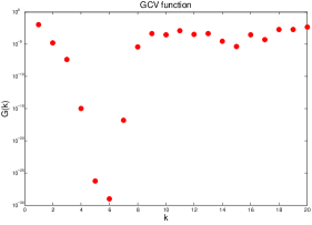
(a) The GCV function

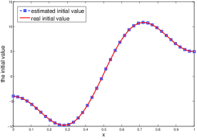
(b) The initial value

Figure 2: The GCV function and initial value

Finally, based on the error analysis in the previous section, we can give the bound of the error between the real value $\alpha$ and the reconstructed one $\widetilde{\alpha}=4.0000$. The parameters that are relevant to the error analysis are given in Table 3.

Table 3: The parameters for error analysis

$M_{0}$	$\alpha_{0}$	$M$	$N$	$L$	$T_{1}$	$T_{s}$	$\theta$	$M_{\theta,L}$	$\|Y_{1}\|_{2}$
15	3	2	50	17	0.3	0.01	2.3687	0.0936	11.8427

$\sigma_{M}$	$\|Y_{0,M}-Y_{0}\|_{2}$	$\kappa(X_{M})$	$\rho$
$9.5089\times 10^{-5}$	$2.2494\times 10^{-15}$	17.9467	$1.4522\times 10^{-10}$

By Theorem 4.2,

$$|\widetilde{z}_{n}-z_{n}|<\displaystyle\frac{\kappa(X_{M})\cdot\rho}{\sigma_{M}\cdot(1-\rho)}\cdot\left[\displaystyle\frac{1+\sqrt{5}}{2}\|Y_{1}\|_{2}+\sigma_{M}\right]\approx 5.2521\times 10^{-4}\triangleq e,\;n\in{\mathbb{K}}_{M}=\{0,1\}.$$ (5.5)

It is clear from Table 2(a) that $\widetilde{z}_{1}=\widetilde{z}_{n_{1}}=0.6738\gg e,$ and it follows from (4.30) in Remark 4.1 that

$$|\alpha-\widetilde{\alpha}|=\displaystyle\frac{|\lambda_{1}-\widetilde{\lambda}_{1}|}{\pi^{2}}<\displaystyle\frac{e}{\pi^{2}\cdot T_{s}\cdot\widetilde{z}_{1}}\approx 7.8974\times 10^{-3}.$$ (5.6)

We thus know that the real diffusion coefficient $\alpha^{\ast}$ is between 3.9921 and 4.0079.

6 Concluding remarks

In this paper, we represent the boundary observation with boundary Neumann control for a one-dimensional heat equation into a Dirichlet series in terms of spectrum determined by the diffusivity and coefficients determined by the initial value. The identification of diffusion coefficient and initial value is therefore transformed into an inverse problem of reconstruction of spectrum-coefficient data from the observation. Taking the first finite terms of the series, the problem happens to be an inverse problem of finite exponential sequence with deterministic small perturbation. We are thus able to develop an algorithm to reconstruct simultaneously the diffusion coefficient and initial value by the matrix pencil method which is used in signal processing. An error analysis is presented and a numerical experiment is carried out to validate the efficiency and accuracy of the proposed algorithm. The method developed is promising and can be applied in identification of variable coefficients and other PDEs.

References

- [1] M. Abramowitz and I.A. Stegun, Handbook of Mathematical Functions with Formulas, Graphs, and Mathematical Tables, Dover Publications, New York, 1964.
- [2] F.L. Bauer and C.T. Fike, Norms and exclusion theorems, Numer. Math., 2(1960), 137–141.
- [3] A. Benabdallah, P. Gaitan, and J.L. Rousseau, Stability of discontinuous diffusion coefficients and initial conditions in an inverse problem for the heat equation, SIAM J. Control Optim., 46(2007), 1849-1881.
- [4] J.D. Chang and B.Z. Guo, Identification of variable spacial coefficients for a beam equation from boundary measurements, Automatica, 43(2007), 732–737.
- [5] M. Choulli and M. Yamamoto, Uniqueness and stability in determining the heat radiative coefficient, the initial temperature and a boundary coefficient in a parabolic equation, Nonlinear Anal., 69(2008), 3983-3998.
- [6] Z.C. Deng, L. Yang and J.N. Yu, Identifying the radiative coefficient of heat conduction equations from discrete measurement data, Appl. Math. Lett., 22(2009), 495-500.
- [7] G.H. Golub, M. Heath and G. Wahba, Generalized cross-validation as a method for choosing a good ridge parameter, Technometrics, 21(1979), 215-223.
- [8] B.Z. Guo and J.D. Chang, Simultaneous identifiability of coefficients, initial state and source for string and beam equations via boundary control and observation, Proc. 8th Asian Control Conference, Kaohsiung, 2011, 365–370.
- [9] S. Gutman and J.H. Ha, Identifiability of piecewise constant conductivity in a heat conduction process, SIAM J. Control Optim., 46(2007), 694–713.
- [10] P.C. Hansen, Discrete Inverse Problems: Insight and Algorithms, SIAM, Philadelphia, 2010.
- [11] Y.B. Hua and T.K. Sarkar, Further analysis of three modern techniques for pole retrieval from data sequence, Proc. 30th Midwest Symp. Circuits Syst., Syracuse, NY, Aug. 1987, 793-797.
- [12] Y.B. Hua and T.K. Sarkar, Matrix pencil method and its performance, Proc. IEEE Int. Conf. Acoust., Speech, Signal Processing, NY, Apr. 1988, 2476-2479.
- [13] Y.B. Hua and T.K. Sarkar, Matrix pencil method for estimating parameters of exponentially damped/undamped sinusoids in noise, IEEE Trans. Acoust. Speech Signal Process., 38(1990), 814–824.
- [14] V. Isakov, Inverse Problems for Partial Differential Equations, Springer, New York, 1998.
- [15] A. Kirsch, An Introduction to the Mathematical Theory of Inverse Problems, Springer, New York, 1999.
- [16] S. Kitamura and S. Nakagiri, Identifiability of spatially-varying and constant parameters in distributed systems of parabolic type, SIAM J. Contorl Optim., 15(1977), 785–802.
- [17] B.M. Levitan, Inverse Sturm-Liouville Problems, VNU Science Press, Utrecht, 1987.
- [18] A. Lorenzi, Identification of the thermal conductivity in the nonlinear heat equation, Inverse Problems, 3(1987), 437-451.
- [19] Y.J. Ma, C.L. Fu, and Y.X. Zhang, Identification of an unknown source depending on both time and space variables by a variational method, Appl. Math. Model., 36(2012), 5080–5090.
- [20] L. Mirsky, Symmetric gauge functions and unitarily invariant norms, Quart. J. Math. Oxford Ser. (2), 11(1960), 50–59.
- [21] R. Murayama, The Gel’fand-Levitan theory and certain inverse problmes for the parabolic equation, J. Fac. Sci. Univ. Tokyo Sect. IA Math., 28(1981), 317–330.
- [22] S. Nakagiri, Identifiability of linear systems in Hilbert spaces, SIAM J. Contorl Optim., 21(1983), 501–530.
- [23] Y. Orlov and J. Bentsman, Adaptive distributed parameter systems identification with enforceable identifiability conditions and reduced-order spatial differentiation, IEEE Trans. Automat. Control, 45(2000), 203–216.
- [24] A. Pierce, Unique identification of eigenvalues and coefficients in a parabolic equation, SIAM J. Contorl Optim., 17(1979), 494–499.
- [25] J. Pöschel and E. Trubowitz, Inverse Spectral Theory, Academic Press, Orlando, 1987.
- [26] K. Ramdani, M. Tucsnak, and G. Weiss, Recovering the initial state of an infinite-dimensional system using observers, Automatica, 46(2010), 1616–1625.
- [27] A. Smyshlyaev, Y. Orlov and M. Krstic, Adaptive identification of two unstable PDEs with boundary sensing and actuation, Int. J. Adapt. Control Signal Process., 23(2009), 131–149.
- [28] G.W. Stewart, On the perturbation of pseudo-inverses, projections and linear least squares problems, SIAM Rev., 19(1977), 634–662.
- [29] T. Suzuki and R. Murayama, A uniqueness theorem in an identification problem for coefficients of parabolic equations, Proc. Japan Acad. Ser. A Math. Sci., 56(1980), 259–363.
- [30] T. Suzuki, Uniqueness and nonuniqueness in an inverse problem for the parabolic equation, J. Differential Equations, 47(1983), 296–316.
- [31] E.C. Titchmarsh, Introduction to the Theory of Fourier Integrals, 2nd Edtion, Clarendon Press, Oxford, 1948.
- [32] Y.B. Wang, J. Cheng, J. Nakagawa, and M. Yamamoto, A numerical method for solving the inverse heat conduction problem without initial value, Inverse Probl. Sci. Eng., 18(2010), 655–671.
- [33] P.A. Wedin, Perturbation theory for pseudo-inverses, BIT, 13(1973), 217–232.
- [34] G.Q. Xu, State reconstruction of a distributed parameter system with exact observability, J. Math. Anal. Appl., 409(2014), 168–179.
- [35] M. Yamamoto and J. Zou, Simultaneous reconstruction of the initial temperature and heat radiative coefficient, Inverse Problems, 17(2001), 1181–1202.
- [36] M. Yamamoto, Carleman estimates for parabolic equations and applications, Inverse Problems, 25(2009), 123013 (75pp).
- [37] G.H. Zheng and T. Wei, Recovering the source and initial value simultaneously in a parabolic equation, Inverse Problems, 30(2014), 065013 (35pp).