UTHEP-686

Light-cone gauge superstring field theory in linear dilaton background

Nobuyuki Ishibashi

Center for Integrated Research in Fundamental Science and Engineering (CiRfSE),

Faculty of Pure and Applied Sciences, University of Tsukuba

Tsukuba, Ibaraki 305-8571, JAPAN

The Feynman amplitudes of light-cone gauge superstring field theory suffer from various divergences. In order to regularize them, we study the theory in linear dilaton background $\Phi=-iQX^{1}$ with the number of spacetime dimensions fixed. We show that the theory with the Feynman $i\varepsilon\,(\varepsilon>0)$ and $Q^{2}>10$ yields finite results.

1 Introduction

Light-cone gauge superstring field theory [1, 2, 3, 4, 5, 6] was proposed to give a nonperturbative definition of closed superstring theory with only three-string interaction terms. However it is known that the Feynman amplitudes of the theory are plagued with various divergences. Even the tree amplitudes are ill defined because of the so-called contact term divergences [7, 8, 9, 10] caused by the insertions of world sheet supercurrents at the interaction points.

In our previous works [11, 12, 13, 14, 15, 16, 17, 18, 19], we have proposed dimensional regularization to deal with the contact term divergences of the light-cone gauge superstring field theory in the RNS formalism. Since the light-cone gauge theory is a completely gauge fixed theory, it is possible to formulate it in $d$ dimensional Minkowski space with $d\neq 10$. Although Lorentz invariance is broken, the theory corresponds to a conformal gauge world sheet theory with nonstandard longitudinal part. The world sheet theory for the longitudinal variables turns out to be a superconformal field theory with the right central charge so that we can construct nilpotent BRST charge. The contributions from the longitudinal part of the world sheet theory, or equivalently the anomaly factors which appear in the light-cone gauge Feynman amplitudes, have the effect of taming the contact term divergences and the tree amplitudes become finite when $-d$ is large enough. It is possible to define the amplitudes as analytic functions of $d$ and take the limit $d\to 10$ to get the amplitudes for critical strings. The results coincide with those of the first quantized formalism.

We expect that the dimensional regularization or its variant also works as a regularization of the multiloop amplitudes. In order to generalize our results to the multiloop case, there are several things to be done. We need to study how divergences of multiloop amplitudes arise in light-cone gauge perturbation theory and check if they are regularized by considering the theory in noncritical dimension. Another problem to be considered is how to deal with the spacetime fermions. Naive dimensional regularization causes problems about spacetime fermions because the number of gamma matrices is modified in the regularization.

In this paper, we propose superstring field theory in linear dilaton background to regularize the divergences of the multiloop amplitudes. With the linear dilaton background keeping the number of transverse coordinates to be eight, we can tame the divergences without having problems about fermions. A Feynman amplitude is given as an integral over moduli parameters and the integrand is written in terms of quantities defined on the light-cone diagram. The divergences originate from degenerations of the world sheet and collisions of interaction points. We prove that with the Feynman $i\varepsilon\,(\varepsilon>0)$ and the background charge $Q$ satisfying $Q^{2}>10$, the amplitudes become finite. It should be possible to define the amplitudes as analytic functions of $Q$ for $Q^{2}>10$ and take the limit $Q\to 0$ to obtain those in the critical dimension. What happens in the limit is the subject of another paper [20].

The organization of this paper is as follows. In section 2, we construct the superstring theory in linear dilaton background and present the perturbative amplitudes obtained from the theory. In section 3, we study the light-cone diagrams which contain divergences. Divergences originate from degeneration of the world sheet and collisions of interaction points. We study how light-cone diagrams corresponding to degenerate Riemann surfaces look like. In section 4, we examine the singular contributions to the amplitudes from the light-cone diagrams in which degenerations and collisions of interaction points occur. In section 5, we show that the amplitudes are finite for the theory with the Feynman $i\varepsilon\,(\varepsilon>0)$ and the background charge $Q$ satisfying $Q^{2}>10$. Section 6 is devoted to discussions.

2 Superstring field theory in linear dilaton background

2.1 Light-cone gauge superstring field theory

In light-cone gauge closed superstring field theory, the string field

$$\left|\Phi\left(t,\alpha\right)\right\rangle$$

is taken to be an element of the Hilbert space of the transverse variables on the world sheet and a function of

$$t = x^{+}\,,$$

$$\alpha = 2p^{+}\,.$$

In this paper, we consider the superstring theory in the RNS formalism. $\left|\Phi(t,\alpha)\right\rangle$ should be GSO even and satisfy the level matching condition

$$(L_{0}-\bar{L}_{0})\left|\Phi\left(t,\alpha\right)\right\rangle=0\,,$$ (2.1)

where $L_{0},\bar{L}_{0}$ are the Virasoro generators of the world sheet theory.

In type II superstring theory, the Hilbert space consists of (NS,NS), (NS,R), (R,NS) and (R,R) sectors and the string fields in the (NS,NS) and (R,R) sectors are bosonic and those in the (NS,R), (R,NS) sectors are fermionic. In the heterotic case, there are NS and R sectors of the right-moving modes, which correspond to bosonic and fermionic fields respectively. In the following, we will consider the case of type II theory based on a world sheet theory for the transverse variables with central charge

$$c=\frac{3}{2}(d-2)\,.$$

The heterotic case can be dealt with in a similar way.

The action of the string field theory is given by [11, 21]

$$S = \int dt\left[\frac{1}{2}\sum_{\mathrm{B}}\int_{-\infty}^{\infty}\frac{\alpha d\alpha}{4\pi}\left\langle\Phi_{\mathrm{B}}\left(-\alpha\right)\right|(i\partial_{t}-\frac{L_{0}+\bar{L}_{0}-\frac{d-2}{8}-i\varepsilon}{\alpha})\left|\Phi_{\mathrm{B}}\left(\alpha\right)\right\rangle\right.$$ (2.2)

$$\hphantom{\int dt\quad}+\frac{1}{2}\sum_{\mathrm{F}}\int_{-\infty}^{\infty}\frac{d\alpha}{4\pi}\left\langle\Phi_{\mathrm{F}}\left(-\alpha\right)\right|(i\partial_{t}-\frac{L_{0}+\bar{L}_{0}-\frac{d-2}{8}-i\varepsilon}{\alpha})\left|\Phi_{\mathrm{F}}\left(\alpha\right)\right\rangle$$

$$\hphantom{\int dt\quad}-\frac{g_{s}}{6}\sum_{\mathrm{B}_{1},\mathrm{B}_{2},\mathrm{B}_{3}}\int\prod_{r=1}^{3}\left(\frac{\alpha_{r}d\alpha_{r}}{4\pi}\right)\delta\left(\sum_{r=1}^{3}\alpha_{r}\right)\left\langle V_{3}\left|\Phi_{\mathrm{B}_{1}}(\alpha_{1})\right.\right\rangle\left|\Phi_{\mathrm{B}_{2}}(\alpha_{2})\right\rangle\left|\Phi_{\mathrm{B}_{3}}(\alpha_{3})\right\rangle$$

$$\hphantom{\int dt\quad}\left.-\frac{g_{s}}{2}\sum_{\mathrm{B}_{1},\mathrm{F}_{2},\mathrm{F}_{3}}\int\prod_{r=1}^{3}\left(\frac{\alpha_{r}d\alpha_{r}}{4\pi}\right)\delta\left(\sum_{r=1}^{3}\alpha_{r}\right)\left\langle V_{3}\left|\Phi_{\mathrm{B}_{1}}(\alpha_{1})\right.\right\rangle\alpha_{2}^{-\frac{1}{2}}\left|\Phi_{\mathrm{F}_{2}}(\alpha_{2})\right\rangle\alpha_{3}^{-\frac{1}{2}}\left|\Phi_{\mathrm{F}_{3}}(\alpha_{3})\right\rangle\right]\,.$$

The first and the second terms are the kinetic terms with the Feynman $i\varepsilon$ and $\left\langle\Phi(-\alpha)\right|$ denotes the BPZ conjugate of $\left|\Phi(-\alpha)\right\rangle$. The third and the fourth terms are the three string vertices and $g_{s}$ is the string coupling constant. $\sum_{\mathrm{B}}$ and $\sum_{\mathrm{F}}$ denote the sums over bosonic and fermionic string fields respectively.

By the state-operator correspondence of the world sheet conformal field theory, there exists a local operator $\mathcal{O}_{\Phi}(\xi,\bar{\xi})$ corresponding to any state $\left|\Phi\right\rangle$. We define $\left\langle\left.V_{3}\right|\Phi(\alpha_{1})\right\rangle\left|\Phi(\alpha_{2})\right\rangle\left|\Phi(\alpha_{3})\right\rangle$ with $\sum_{r=1}^{3}\alpha_{r}=0$ to be

$$\left\langle\left.V_{3}\right|\Phi(\alpha_{1})\right\rangle\left|\Phi(\alpha_{2})\right\rangle\left|\Phi(\alpha_{3})\right\rangle$$

$$\quad=\left\langle\lim_{\rho\to\rho_{0}}\left|\rho-\rho_{0}\right|^{\frac{3}{2}}T_{F}^{LC}\left(\rho\right)\bar{T}_{F}^{LC}\left(\bar{\rho}\right)h_{1}\circ\mathcal{O}_{\Phi\left(\alpha_{1}\right)}(0,0)h_{2}\circ\mathcal{O}_{\Phi\left(\alpha_{2}\right)}(0,0)h_{3}\circ\mathcal{O}_{\Phi\left(\alpha_{3}\right)}(0,0)\right\rangle_{\Sigma}\,,$$ (2.3)

in terms of a correlation function on $\Sigma$ which is the world sheet describing the three string interaction depicted in Fig. 1. On each cylinder corresponding to an external line, one can introduce a complex coordinate

$$\rho=\tau+i\sigma\,,$$

whose real part $\tau$ coincides with the Wick rotated light-cone time $it$ and imaginary part $\sigma\sim\sigma+2\pi\alpha_{r}$ parametrizes the closed string at each time. The $\rho$’s on the cylinders are smoothly connected except at the interaction point $\rho_{0}$ and we get a complex coordinate $\rho$ on $\Sigma$. The correlation function $\left\langle\cdot\right\rangle_{\Sigma}$ is defined with the metric

$$ds^{2}=d\rho d\bar{\rho}\,,$$

on the world sheet. $h_{r}(\xi)$ gives a map from a unit disk $\left|\xi\right|<1$ to the cylinder corresponding to the $r$-th external line so that

$$\xi=e^{\frac{1}{\alpha_{r}}(h_{r}(\xi)-\rho_{0})}\,.$$

$T_{F}^{LC},\bar{T}_{F}^{LC}$ are the supercurrents of the transverse world sheet theory.

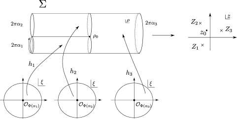
Figure 1: The three string vertex for superstrings. Here we consider the case $\alpha_{1},\alpha_{2}>0,\,\alpha_{3}<0$.

It is convenient to express the right hand side of (2.3) in terms of a correlation function on the sphere as

$$\left\langle\left.V_{3}\right|\Phi(\alpha_{1})\right\rangle\left|\Phi(\alpha_{2})\right\rangle\left|\Phi(\alpha_{3})\right\rangle$$

$$\quad=e^{-\frac{d-2}{16}\Gamma}\left\langle\left|\partial^{2}\rho\left(z_{0}\right)\right|^{-\frac{3}{2}}T_{F}^{LC}\left(z_{0}\right)\bar{T}_{F}^{LC}\left(\bar{z}_{0}\right)\right.$$

$$\hphantom{\quad=e^{-\frac{d-2}{16}\Gamma}T_{F}^{LC}\left(z_{0}\right)}\times\left.\rho^{-1}h_{1}\circ\mathcal{O}_{\Phi_{1}\left(\alpha_{1}\right)}(0,0)\rho^{-1}h_{2}\circ\mathcal{O}_{\Phi_{2}\left(\alpha_{2}\right)}(0,0)\rho^{-1}h_{3}\circ\mathcal{O}_{\Phi_{3}\left(\alpha_{3}\right)}(0,0)\right\rangle_{\mathbb{C}\cup\infty}\,.$$ (2.4)

Here $\rho(z)$ is given by

$$\rho(z)=\sum_{r=1}^{3}\alpha_{r}\ln(z-Z_{r})\,,$$

which maps the complex plane to $\Sigma$. $z_{0}$ denotes the $z$-coordinate of the interaction point, which satisfies

$$\partial\rho(z_{0})=0\,.$$

The correlation function $\left\langle\cdot\right\rangle_{\mathbb{C}\cup\infty}$ is defined with the metric

$$ds^{2}=dzd\bar{z}\,,$$

on the world sheet. The salient feature of light-cone gauge string field theory is that the central charge of the world sheet theory is nonvanishing even in the critical case. $e^{-\frac{d-2}{16}\Gamma}$ is the anomaly factor associated to the conformal map $z\to\rho(z)$ and its explicit form is given as

$$e^{-\frac{d-2}{16}\Gamma}=\left(\frac{\exp\left(-2\sum_{r}\frac{\hat{\tau}_{0}}{\alpha_{r}}\right)}{\alpha_{1}\alpha_{2}\alpha_{3}}\right)^{\frac{d-2}{16}}\,,$$

where

$$\hat{\tau}_{0}\equiv\sum_{r=1}^{3}\alpha_{r}\ln\left|\alpha_{r}\right|\,.$$

2.2 Linear dilaton background

The Feynman amplitudes of light-cone gauge superstring field theory suffer from the contact term divergences. As we have pointed out in [11], these divergences are regularized by formulating the theory in $d\neq 10$ dimensions. However, if one simply considers superstring field theory in noncritical dimensions, fermionic string fields cannot satisfy (2.1) [15]. In type II superstring theory, naive dimensional continuation implies that the level-matching condition for the (NS,R) sector becomes

$$\mathcal{N}+\frac{d-2}{16}=\bar{\mathcal{N}}\,,$$

where $\mathcal{N}$ and $\bar{\mathcal{N}}$ denote the left and right mode numbers of the light-cone gauge string state. For generic $d$, there exists no state satisfying it. The same argument applies to (R,NS) sector. We have the same problem in the R sector of the heterotic string theory. Therefore we cannot use the naive dimensional regularization to regularize superstring amplitudes, although it may be used to deal with the type 0 theories. Another drawback of the naive dimensional regularization is that there is difficulty in dealing with odd spin structure , as anticipated from the problems with $\gamma^{5}$ in the dimensional regularization in field theory.

It is possible to regularize the divergences by formulating the theory based on world sheet theory with a large negative central charge, instead of changing the number of spacetime dimensions. Therefore, in order to have a theory without the aforementioned problems, we need a world sheet theory in which we can change the central charge keeping the number of the world sheet fermions fixed. A convenient way to obtain such a theory is to take the dilaton background to be $\Phi=-iQX^{1}$, proportional to one of the transverse target space coordinates $X^{1}$. Then the world sheet action of $X^{1}$ and its fermionic partners $\psi^{1},\bar{\psi^{1}}$ on a world sheet with metric $ds^{2}=2\hat{g}_{z\bar{z}}dzd\bar{z}$ becomes

$$S\left[X^{1},\psi^{1},\bar{\psi}^{1};\hat{g}_{z\bar{z}}\right] = \frac{1}{16\pi}\int dz\wedge d\bar{z}i\sqrt{\hat{g}}\left(\hat{g}^{ab}\partial_{a}X^{1}\partial_{b}X^{1}-2iQ\hat{R}X^{1}\right)$$ (2.5)

$$\qquad+\frac{1}{4\pi}\int dz\wedge d\bar{z}i\left(\psi^{1}\bar{\partial}\psi^{1}+\bar{\psi}^{1}\partial\bar{\psi}^{1}\right)\,,$$

and the energy-momentum tensor and the supercurrent are given as

$$T^{X^{1}}(z) = -\frac{1}{2}(\partial X^{1})^{2}-iQ(\partial-\partial\ln\hat{g}_{z\bar{z}})\partial X^{1}-\frac{1}{2}\psi^{1}\partial\psi^{1}\,,$$

$$T_{F}^{X^{1}}(z) = -\frac{i}{2}\partial X^{1}\psi^{1}+Q(\partial-\frac{1}{2}\partial\ln\hat{g}_{z\bar{z}})\psi^{1}\,.$$

In this paper, we take $Q$ to be a real constant.

In order to construct string field theory and calculate amplitudes we need the correlation functions of the linear dilaton conformal field theory. Since the fermionic part is just a free theory we concentrate on the bosonic part. Let us consider the correlation function of operators $e^{ip_{r}X^{1}}\,(r=1,\cdots,N)$ on a Riemann surface of genus $g$ with metric $ds^{2}=2g_{z\bar{z}}dzd\bar{z}$, which is given as

$$\int\left[dX^{1}\right]_{g_{z\bar{z}}}e^{-S\left[X^{1};g_{z\bar{z}}\right]}\prod_{r=1}^{N}e^{ip_{r}X^{1}}(Z_{r},\bar{Z}_{r})\,,$$ (2.6)

where

$$S\left[X^{1};g_{z\bar{z}}\right]=\frac{1}{16\pi}\int dz\wedge d\bar{z}i\sqrt{g}\left(g^{ab}\partial_{a}X^{1}\partial_{b}X^{1}-2iQRX^{1}\right)\,.$$

We would like to express (2.6) in terms of the correlation function on the world sheet with a fiducial metric $ds^{2}=2\hat{g}_{z\bar{z}}dzd\bar{z}$. It is straightforward to show

$$\int\left[dX^{1}\right]_{g_{z\bar{z}}}e^{-S\left[X^{1};g_{z\bar{z}}\right]}\prod_{r=1}^{N}e^{ip_{r}X^{1}}(Z_{r},\bar{Z}_{r})$$

$$\quad=e^{-\frac{1-12Q^{2}}{24}\Gamma\left[\sigma;\hat{g}_{z\bar{z}}\right]}\int\left[d\hat{X}{}^{1}\right]_{\hat{g}_{z\bar{z}}}e^{-S\left[\hat{X}^{1};\hat{g}_{z\bar{z}}\right]}\prod_{r=1}^{N}\left[e^{ip_{r}\hat{X}^{1}}\left(\frac{g_{z\bar{z}}}{\hat{g}_{z\bar{z}}}\right)^{-Qp_{r}}\right](Z_{r},\bar{Z}_{r})\,,$$

where

$$\sigma \equiv \ln g_{z\bar{z}}-\ln\hat{g}_{z\bar{z}}\,,$$

$$\Gamma\left[\sigma;\hat{g}_{z\bar{z}}\right] = -\frac{1}{4\pi}\int dz\wedge d\bar{z}i\sqrt{\hat{g}}\left(\hat{g}^{ab}\partial_{a}\sigma\partial_{b}\sigma+2\hat{R}\sigma\right)\,,$$ (2.7)

$$\hat{X}^{1} \equiv X^{1}-iQ\sigma\,.$$

The anomaly factor $e^{-\frac{1-12Q^{2}}{24}\Gamma\left[\sigma;\hat{g}_{z\bar{z}}\right]}$ is exactly what we expect for a theory with the central charge

$$c=1-12Q^{2}$$

of the linear dilaton conformal field theory. The correlation functions with the fiducial metric $ds^{2}=2\hat{g}_{z\bar{z}}dzd\bar{z}$ can be calculated by introducing the Arakelov Green’s function $G^{\mathrm{A}}(z,w)$ [22] which satisfies

$$\partial_{z}\partial_{\bar{z}}G^{\mathrm{A}}(z,w)=-\pi\delta^{2}(z-w)-\frac{\hat{g}_{z\bar{z}}\hat{R}}{4(g-1)}\,,$$

$$\int dz\wedge d\bar{z}i\sqrt{\hat{g}}\hat{R}G^{\mathrm{A}}(z,w)=0\,,$$

and the result is

$$\int\left[d\hat{X}^{1}\right]_{\hat{g}_{z\bar{z}}}e^{-S\left[\hat{X}^{1};\hat{g}_{z\bar{z}}\right]}\prod e^{ip_{r}^{1}\hat{X}}(Z_{r},\bar{Z}_{r})$$

$$\quad=2\pi\delta\left(\sum p_{r}+2Q(1-g)\right)Z^{X}\left[\hat{g}_{z\bar{z}}\right]$$

$$\hphantom{\quad=\quad}\times\prod_{r>s}e^{-p_{r}p_{s}G^{\mathrm{A}}(Z_{r},Z_{s})}\prod_{r}e^{-\frac{1}{2}p_{r}^{2}\lim_{z\to Z_{r}}(G^{\mathrm{A}}(z,Z_{r})+\ln\left|z-Z_{r}\right|^{2})}\,.$$

Here $Z^{X}\left[\hat{g}_{z\bar{z}}\right]$ denotes the partition function of a free scalar on the world sheet with metric $ds^{2}=2\hat{g}_{z\bar{z}}dzd\bar{z}$. Taking the fiducial metric to be the Arakelov metric $g_{z\bar{z}}^{\mathrm{A}}$ [22], for which the Arakelov Green’s function $G^{\mathrm{A}}(z,w)$ satisfies

$$\lim_{w\to z}\left(G^{\mathrm{A}}(w,z)+\ln\left|z-w\right|^{2}\right)=-\ln\left(2g_{z\bar{z}}^{\mathrm{A}}\right)\,,$$

the correlation function becomes

$$2\pi\delta\left(\sum p_{r}+2Q(1-g)\right)Z^{X}\left[g_{z\bar{z}}^{\mathrm{A}}\right]\prod_{r>s}e^{-p_{r}p_{s}G^{\mathrm{A}}(Z_{r},Z_{s})}\prod_{r}\left(2g_{Z_{r}\bar{Z}_{r}}^{\mathrm{A}}\right)^{\frac{1}{2}p_{r}^{2}}\,.$$

From these calculations, we can see that it is convenient to define

$$\tilde{X}^{1}\equiv X^{1}-iQ\ln(2g_{z\bar{z}})\,,$$

so that the correlation function of $e^{ip_{r}\tilde{X}^{1}}(Z_{r},\bar{Z}_{r})\,(r=1,\cdots,N)$ is expressed as

$$\int\left[dX^{1}\right]_{g_{z\bar{z}}}e^{-S\left[X^{1};g_{z\bar{z}}\right]}\prod_{r=1}^{N}e^{ip_{r}\tilde{X}^{1}}(Z_{r},\bar{Z}_{r})$$

$$\quad=2\pi\delta\left(\sum p_{r}+2Q(1-g)\right)e^{-\frac{1-12Q^{2}}{24}\Gamma\left[\sigma;g_{z\bar{z}}^{\mathrm{A}}\right]}Z^{X}\left[g_{z\bar{z}}^{\mathrm{A}}\right]\prod_{r>s}e^{-p_{r}p_{s}G^{\mathrm{A}}(Z_{r},Z_{s})}\prod_{r}\left(2g_{Z_{r}\bar{Z}_{r}}^{\mathrm{A}}\right)^{\frac{1}{2}p_{r}^{2}+Qp_{r}}\,.$$

(2.8)

On the sphere, this becomes

$$\int\left[dX^{1}\right]_{g_{z\bar{z}}}e^{-S\left[X^{1};g_{z\bar{z}}\right]}\prod_{r=1}^{N}e^{ip_{r}\tilde{X}^{1}}(Z_{r},\bar{Z}_{r})$$

$$\quad=2\pi\delta\left(\sum p_{r}+2Q\right)e^{-\frac{1-12Q^{2}}{24}\Gamma\left[\sigma;g_{z\bar{z}}^{\mathrm{A}}\right]}\prod_{r>s}\left|Z_{r}-Z_{s}\right|^{2p_{r}p_{s}}\,.$$ (2.9)

$e^{ip\tilde{X}^{1}}$ thus defined turns out to be a primary field with conformal dimension

$$\frac{1}{2}p^{2}+Qp=\frac{1}{2}(p+Q)^{2}-\frac{Q^{2}}{2}\,.$$ (2.10)

Notice that $\tilde{X}^{1}$ satisfies

$$\partial\bar{\partial}\tilde{X}^{1}=0\,,$$

if there are no source terms and $i\partial\tilde{X}^{1}(z),i\bar{\partial}\tilde{X}^{1}(\bar{z})$ can be expanded as

$$i\partial\tilde{X}^{1}(z) = \sum_{n}\alpha_{n}^{1}z^{-n-1}\,,$$

$$i\bar{\partial}\tilde{X}^{1}(\bar{z}) = \sum_{n}\bar{\alpha}_{n}^{1}\bar{z}^{-n-1}\,,$$

where $\alpha_{n}^{1}$ and $\bar{\alpha}_{n}^{1}$ satisfy the canonical commutation relations. The states in the CFT can be expressed as linear combinations of the Fock space states

$$\alpha_{-n_{1}}^{1}\cdots\alpha_{-n_{k}}^{1}\bar{\alpha}_{-\bar{n}_{1}}^{1}\cdots\bar{\alpha}_{-\bar{n}_{l}}^{1}\left|p\right\rangle\,.$$ (2.11)

It is straightforward to show

$$\langle p_{1}|p_{2}\rangle = 2\pi\delta(p_{1}+p_{2}+2Q)\,,$$

$$\left(\alpha_{n}^{1}\right)^{\ast} = (-1)^{n+1}(\alpha_{-n}^{1}+2Q\delta_{n,0})\,,$$

$$\left(\bar{\alpha}_{n}^{1}\right)^{\ast} = (-1)^{n+1}(\bar{\alpha}_{-n}^{1}+2Q\delta_{n,0})\,,$$

where $\left\langle p\right|,\left(\alpha_{n}^{1}\right)^{\ast},\left(\bar{\alpha}_{n}^{1}\right)^{\ast}$ are the BPZ conjugates of $\left|p\right\rangle,\alpha_{n}^{1},\bar{\alpha}_{n}^{1}$ respectively.

2.3 Light-cone gauge superstring field theory in linear dilaton background

Now let us construct the light-cone gauge superstring field theory based on the world sheet theory with the variables

$$X^{i},\psi^{i},\bar{\psi}^{i}\ (i=1,\cdots,8)\,,$$

where the action for $X^{1},\psi^{1},\bar{\psi}^{1}$ is taken to be (2.5) and that for other variables is the free one. The world sheet theory of the transverse variables turns out to be a superconformal field theory with central charge

$$c=12-12Q^{2}\,.$$

Therefore we can make $-c$ arbitrarily large keeping the number of the transverse fermionic variables fixed. From the correlation functions (2.9) of the conformal field theory, it is straightforward to construct the light-cone gauge string field action (2.2) with

$$d-2=8-8Q^{2}\,.$$

The Feynman amplitudes are calculated by the old-fashioned perturbation theory starting from the action (2.2). Each term in the expansion corresponds to a light-cone gauge Feynman diagram for strings which is constructed from the propagator and the vertex presented in Fig. 2. A typical diagram is depicted in Fig. 3.

Figure 2: Propagator and vertex.

Figure 3: A string diagram with $3$ incoming, $2$ outgoing strings and $3$ loops.

A Wick rotated $g$-loop $N$-string diagram is conformally equivalent to an $N$ punctured genus $g$ Riemann surface $\Sigma_{N}^{(g)}$. A light-cone diagram consists of cylinders which correspond to propagators of the closed string. On each cylinder, one can introduce a complex coordinate $\rho$ as we did for the three string vertex. The $\rho$’s on the cylinders are smoothly connected except at the interaction points and we get a complex coordinate $\rho$ on $\Sigma_{N}^{(g)}$. $\rho$ is not a good coordinate at the punctures and the interaction points.

$\rho$ can be given as a function of a local coordinate $z$ on $\Sigma_{N}^{(g)}$ as [16]

$$\rho(z)=\sum_{r=1}^{N}\alpha_{r}\left[\ln E(z,Z_{r})-2\pi i\int_{P_{0}}^{z}\omega\frac{1}{\mathop{\mathrm{Im}}\Omega}\mathop{\mathrm{Im}}\int_{P_{0}}^{Z_{r}}\omega\right]\leavevmode\nobreak\ ,\qquad\sum_{r=1}^{N}\alpha_{r}=0\leavevmode\nobreak\ ,$$ (2.12)

up to an additive constant independent of $z$. Here $E(z,w)$ is the prime form, $\omega$ is the canonical basis of the holomorphic abelian differentials and $\Omega$ is the period matrix of the surface. The base point $P_{0}$ is arbitrary. There are $2g-2+N$ zeros of $\partial\rho$ and we denote them by $z_{I}\,(I=1,\cdots,2g-2+N)$. They correspond to the interaction points of the light-cone diagram.

A $g$-loop $N$-string amplitude is given as an integral over the moduli space of the string diagram as

$$A_{N}^{(g)}=\left(2\pi\right)^{2}\delta\left(\sum_{r=1}^{N}p_{r}^{+}\right)\delta\left(\sum_{r=1}^{N}p_{r}^{-}\right)(ig_{s})^{2g-2+N}C\sum_{\mathrm{channels}}\int\left[dT\right]\left[\alpha d\theta\right]\left[d\alpha\right]F_{N}^{(g)}\,,$$ (2.13)

where $\int[dT][\alpha d\theta][d\alpha]$ denotes the integration over the moduli parameters and $C$ is the combinatorial factor. In each channel, the integration measure is given as [24]

$$\int[dT][\alpha d\theta][d\alpha]=\prod_{a=1}^{2g-3+N}\left(-i\int_{0}^{\infty}dT_{a}\right)\prod_{A=1}^{g}\int\frac{d\alpha_{A}}{4\pi}\prod_{\mathcal{I}=1}^{3g-3+N}\left(|\alpha_{\mathcal{I}}|\int_{0}^{2\pi}\frac{d\theta_{\mathcal{I}}}{2\pi}\right).$$ (2.14)

Here $T_{a}$’s are heights of the cylinders corresponding to internal lines, $\alpha_{A}$’s denote the widths of the cylinders corresponding to the $+$ components of the loop momenta and $\alpha_{\mathcal{I}}$’s and $\theta_{\mathcal{I}}$’s are the string-lengths and the twist angles of the internal propagators. Summing over channels, with the natural range of these coordinates, the moduli space of the Riemann surface is covered exactly once [31].

The integrand $F_{N}^{(g)}$ in (2.13) is given as

$$F_{N}^{(g)}=\int\left[dX^{i}d\psi^{i}d\bar{\psi}^{i}\right]_{g_{z\bar{z}}}e^{-S\left[X^{i},\psi^{i},\bar{\psi}^{i};g_{z\bar{z}}^{\mathrm{A}}\right]}\prod_{I=1}^{2g-2+N}\left(\left|\partial^{2}\rho\left(z_{I}\right)\right|^{-\frac{3}{2}}T_{F}^{\mathrm{LC}}\left(z_{I}\right)\bar{T}_{F}^{\mathrm{LC}}\left(\bar{z}_{I}\right)\right)\prod_{r=1}^{N}V_{r}^{\mathrm{LC}}(Z_{r},\bar{Z}_{r})\,.$$

Here $V_{r}^{\mathrm{LC}}(Z_{r},\bar{Z}_{r})$ denotes the vertex operator [11] for the $r$-th external line and the insertions of the world sheet supercharges $T_{F}^{\mathrm{LC}}\left(z_{I}\right),\,\bar{T}_{F}^{\mathrm{LC}}\left(\bar{z}_{I}\right)$ originate from those in the three string vertex (2.4). The path integral is defined with the world sheet metric

$$ds^{2}=2g_{z\bar{z}}dzd\bar{z}\equiv\partial\rho\bar{\partial}\bar{\rho}dzd\bar{z}\,.$$ (2.15)

Since $g_{z\bar{z}}$ is singular at $z=z_{I},Z_{r}$, we need to rewrite the path integral in terms of that defined with a metric which is regular everywhere on the world sheet. Taking the world sheet metric to be the Arakelov metric, we get

$$F_{N}^{(g)} = e^{-\frac{1-Q^{2}}{2}\Gamma\left[\sigma;g_{z\bar{z}}^{\mathrm{A}}\right]}\int\left[dX^{i}d\psi^{i}d\bar{\psi}^{i}\right]_{g_{z\bar{z}}^{\mathrm{A}}}e^{-S\left[X^{i},\psi^{i},\bar{\psi}^{i};g_{z\bar{z}}^{\mathrm{A}}\right]}$$ (2.16)

$$\hphantom{e^{-\frac{1-Q^{2}}{2}\Gamma\left[\sigma;g_{z\bar{z}}^{\mathrm{A}}\right]}\int\quad}\times\prod_{I=1}^{2g-2+N}\left(\left|\partial^{2}\rho\left(z_{I}\right)\right|^{-\frac{3}{2}}T_{F}^{\mathrm{LC}}\left(z_{I}\right)\bar{T}_{F}^{\mathrm{LC}}\left(\bar{z}_{I}\right)\right)\prod_{r=1}^{N}V_{r}^{\mathrm{LC}}(Z_{r},\bar{Z}_{r})\,.$$

It is possible to calculate the quantities which appear on the right hand side of (2.16). Substituting (2.15) into (2.7) yields a divergent result for $\Gamma\left[\sigma;g_{z\bar{z}}^{\mathrm{A}}\right]$. We can obtain $e^{-\Gamma\left[\sigma;g_{z\bar{z}}^{\mathrm{A}}\right]}$ up to a divergent numerical factor by regularizing it as was done in [32]. The divergent factor can be absorbed in a redefinition of $g_{s}$ and the vertex operator. $e^{-\Gamma\left[\sigma;g_{z\bar{z}}^{\mathrm{A}}\right]}$ for higher genus surfaces is calculated in [16] to be

$$e^{-\Gamma\left[\sigma;g_{z\bar{z}}^{\mathrm{A}}\right]}\propto e^{-W}\prod_{r}e^{-2\mathop{\mathrm{Re}}\bar{N}_{00}^{rr}}\prod_{I}\left|\partial^{2}\rho\left(z_{I}\right)\right|^{-3}\,,$$

up to a numerical constant which can be fixed by imposing the factorization condition [16]. Here

$$-W \equiv -2\sum_{I<J}G^{\mathrm{A}}\left(z_{I};z_{J}\right)-2\sum_{r<s}G^{\mathrm{A}}\left(Z_{r};Z_{s}\right)+2\sum_{I,r}G^{\mathrm{A}}\left(z_{I};Z_{r}\right)$$

$${}-\sum_{r}\ln\left(2g_{Z_{r}\bar{Z}_{r}}^{\mathrm{A}}\right)+3\sum_{I}\ln\left(2g_{z_{I}\bar{z}_{I}}^{\mathrm{A}}\right)\,.$$

$$\bar{N}_{00}^{rr} \equiv \lim_{z\to Z_{r}}\left[\frac{\rho(z_{I^{(r)}})-\rho(z)}{\alpha_{r}}+\ln(z-Z_{r})\right]$$

$$= \frac{\rho(z_{I^{(r)}})}{\alpha_{r}}-\sum_{s\neq r}\frac{\alpha_{s}}{\alpha_{r}}\ln E(Z_{r},Z_{s})+\frac{2\pi i}{\alpha_{r}}\int_{P_{0}}^{Z_{r}}\omega\frac{1}{\mathop{\mathrm{Im}}\Omega}\sum_{s=1}^{N}\alpha_{s}\mathop{\mathrm{Im}}\int_{P_{0}}^{Z_{s}}\omega\leavevmode\nobreak\ ,$$

and $z_{I^{(r)}}$ denotes the coordinate of the interaction point at which the $r$-th external line interacts. The correlation functions of $X^{1}$ which appear in (2.16) can be derived from (2.8). $Z^{X}\left[g_{z\bar{z}}^{\mathrm{A}}\right]$ and the correlation functions involving other variables have been calculated on higher genus Riemann surfaces in [33, 34, 35, 36, 37].

From the explicit form of these quantities, we can see that $F_{N}^{(g)}$ could become singular if and only if either or both of the following things happen:

1. Some of the interaction points collide with each other.

2. The Riemann surface corresponding to the world sheet degenerates.

When the interaction points collide, $F_{N}^{(g)}$ could become singular because $\partial^{2}\rho$’s at these points become $0$ and $T_{F}$’s have singular OPE’s. Since all the quantities which appear in $F_{N}^{(g)}$ can be expressed explicitly in terms of the theta functions defined on $\Sigma_{N}^{(g)}$, possible singularities of $F_{N}^{(g)}$ also originate from degenerations of the surface. The singularities of $F_{N}^{(g)}$ arise only from these phenomena, because the world sheet theory does not involve variables like superconformal ghost.

Therefore, in order to study the possible divergences of the amplitude $A_{N}^{(g)}$, we need to investigate the light-cone diagrams in which 1 and/or 2 above happen. Light-cone diagrams with collisions of interaction points are easily visualized. We shall study how light-cone diagrams corresponding to degenerate Riemann surfaces look like, in the next section.

3 Light-cone diagrams in the degeneration limits

There are two types of degeneration, i.e. separating and nonseparating. The expressions of various quantities in these limits are given in [39, 40, 41, 42] from which that of $\rho(z)$ can be obtained. The shape of the light-cone diagrams can be deduced from the form of $\rho(z)$.

3.1 Separating degeneration

Let us first consider the separating degeneration in which a Riemann surface $M$ degenerates into two surfaces $M_{1}$ and $M_{2}$ with genera $g_{1}$ and $g_{2}$ respectively. We assume that $M$ corresponds to a light-cone diagram with $N$ external lines, and $N_{1}$ of them belong to $M_{1}$ and $N_{2}$ of them belong to $M_{2}$.

3.1.1 $g_{1}g_{2}\neq 0$

Let us first consider the case when both $g_{1}$ and $g_{2}$ are positive. The degeneration can be described by a model $M_{t}$ constructed as follows:

• Choose points $p_{j}\in M_{j}$ and a neighborhood $U_{j}$ of $p_{j}$ for $j=1,2$. Let $D$ be the unit disk in $\mathbb{C}$ and define $z_{j}:U_{j}\to D$ to be the coordinate of $U_{j}$ such that $z_{j}(p_{j})=0$.

• For $0<r<1$, let $rU_{j}$ be

  $$rU_{j}\equiv\left\{p\in U_{j};\ \left|z_{j}(p)\right|<r\right\}\,.$$

  For $t\in D$, glue together the surfaces $M_{j}/\left|t\right|U_{j}\ (j=1,2)$ by the identification

  $$z_{1}z_{2}=t\,.$$

  The surface obtained is denoted by $M_{t}$. The degeneration limit corresponds to $t\to 0$.

The complex coordinate $\rho_{t}(z)$ on the light-cone diagram corresponding to $M_{t}$ is given by

$$\rho_{t}(z)=\sum_{r=1}^{N}\alpha_{r}\left[\ln E_{t}(z,Z_{r})-2\pi i\int_{P_{0}}^{z}\omega_{t}\frac{1}{\mathop{\mathrm{Im}}\Omega_{t}}\mathop{\mathrm{Im}}\int_{P_{0}}^{Z_{r}}\omega_{t}\right]\,,$$

where $E_{t}(z,w),\,\omega_{t},\,\Omega_{t}$ denote the prime form, the canonical basis of the holomorphic abelian differentials and the period matrix of $M_{t}$ respectively. The base point $P_{0}$ is taken to be included in $M_{1}/\sqrt{\left|t\right|}U_{1}$. We take the punctures $Z_{1},\cdots,Z_{N_{1}}$ to belong to $M_{1}/\sqrt{\left|t\right|}U_{1}$ and the punctures $Z_{N_{1}+1},\cdots,Z_{N}$ to belong to $M_{2}/\sqrt{\left|t\right|}U_{2}$. Using the formulas of various quantities for $\left|t\right|\ll 1$ given in [39, 40, 41, 42], it is possible to show that $\rho_{t}(x_{1}),\rho_{t}(x_{2})$ for $x_{j}\in M_{j}/\sqrt{\left|t\right|}U_{j}$ become

$$\rho_{t}(x_{1}) = \rho^{(1)}(x_{1})+\sum_{r_{2}=N_{1}+1}^{N}\alpha_{r_{2}}\ln E_{2}(p_{2},Z_{r_{2}})-\frac{\alpha_{p_{1}}}{2}\ln(-t)+\cdots\,,$$

$$\rho_{t}(x_{2}) = \rho^{(2)}(x_{2})+\sum_{r_{1}=1}^{N_{1}}\alpha_{r_{1}}\ln E_{1}(p_{1},Z_{r_{1}})-\frac{\alpha_{p_{2}}}{2}\ln(-t)$$ (3.1)

$$\quad+2\pi i\int_{P_{0}^{\prime}}^{p_{2}}\omega^{(2)}\frac{1}{\mathop{\mathrm{Im}}\Omega_{2}}\mathop{\mathrm{Im}}\left(\sum_{r_{2}=N_{1}+1}^{N}\alpha_{r_{2}}\int_{p_{2}}^{Z_{r_{2}}}\omega^{(2)}+\alpha_{p_{2}}\int_{P_{0}^{\prime}}^{p_{2}}\omega^{(2)}\right)$$

$$\quad-2\pi i\int_{P_{0}}^{p_{1}}\omega^{(1)}\frac{1}{\mathop{\mathrm{Im}}\Omega_{1}}\mathop{\mathrm{Im}}\left(\sum_{r_{1}=1}^{N_{1}}\alpha_{r_{1}}\int_{P_{0}}^{Z_{r_{1}}}\omega^{(1)}+\alpha_{p_{1}}\int_{P_{0}}^{p_{1}}\omega^{(1)}\right)$$

$$\quad+\cdots\,,$$

for $\left|t\right|\ll 1$. Here the ellipses denote the terms higher order in $t$ and

$$\rho^{(1)}(x_{1}) = \sum_{r_{1}=1}^{N_{1}}\alpha_{r_{1}}\ln E_{1}(x_{1},Z_{r_{1}})+\alpha_{p_{1}}\ln E_{1}(x_{1},p_{1})$$

$$\quad-2\pi i\int_{P_{0}}^{x_{1}}\omega^{(1)}\frac{1}{\mathop{\mathrm{Im}}\Omega_{1}}\mathop{\mathrm{Im}}\left(\sum_{r_{1}=1}^{N_{1}}\alpha_{r_{1}}\int_{P_{0}}^{Z_{r_{1}}}\omega^{(1)}+\alpha_{p_{1}}\int_{P_{0}}^{p_{1}}\omega^{(1)}\right)\,,$$

$$\rho^{(2)}(x_{2}) = \sum_{r_{2}=N_{1}+1}^{N}\alpha_{r_{2}}\ln E_{2}(x_{2},Z_{r_{2}})+\alpha_{p_{2}}\ln E_{2}(x_{2},p_{2})$$

$$\quad-2\pi i\int_{P_{0}^{\prime}}^{x_{2}}\omega^{(2)}\frac{1}{\mathop{\mathrm{Im}}\Omega_{2}}\mathop{\mathrm{Im}}\left(\sum_{r_{2}=N_{1}+1}^{N}\alpha_{r_{2}}\int_{P_{0}^{\prime}}^{Z_{r_{2}}}\omega^{(2)}+\alpha_{p_{2}}\int_{P_{0}^{\prime}}^{p_{2}}\omega^{(2)}\right)\,,$$

$$\alpha_{p_{1}} = \sum_{r_{2}=N_{1}+1}^{N}\alpha_{r_{2}}=-\alpha_{p_{2}}=-\sum_{r_{1}=1}^{N_{1}}\alpha_{r_{1}}\,,$$

with $P_{0}^{\prime}\in M_{2}/\sqrt{\left|t\right|}U_{2}$. $E_{j}(z,w),\,\omega^{(j)},\,\Omega_{j}$ denote the prime form, the canonical basis of the holomorphic abelian differentials and the period matrix of $M_{j}\,(j=1,2)$.

From (3.1), we can see how the light-cone diagrams corresponding to the separating degeneration should look like. They are classified according to the values of $\alpha_{p_{1}},N_{1},N_{2}$ as follows:

• $\alpha_{p_{1}}\neq 0$
  If $\alpha_{p_{1}}\neq 0$, $\rho^{(1)},\rho^{(2)}$ can be considered as the coordinates defined on light-cone diagrams with $N^{(1)}+1,\,N^{(2)}+1$ external lines respectively. (3.1) implies that the limit $t\to 0$ corresponds to the one in which the length of an internal line with $\alpha=\alpha_{p_{1}}$ becomes infinite in the light-cone diagram. A light-cone diagram of this type is presented in Fig. 4. $M_{1}$ and $M_{2}$ correspond to light-cone diagrams with the coordinates $\rho^{(1)}$ and $\rho^{(2)}$ respectively.

Figure 4: Light-cone diagram corresponding to a separating degeneration with $\alpha_{p_{1}}\neq 0$.

• $\alpha_{p_{1}}=0,\,N_{1}N_{2}\neq 0$
  When $\alpha_{p_{1}}=0,\,N_{1}N_{2}\neq 0$, higher order terms in (3.1) with respect to $t$ become important. We get

  $$\partial\rho_{t}(x_{1}) \sim \partial\rho^{(1)}(x_{1})-t\partial_{p_{1}}\partial_{x_{1}}\ln E_{1}(x_{1},p_{1})\partial\rho^{(2)}(p_{2})+\cdots\,,$$ (3.2)

  $$\partial\rho_{t}(x_{2}) \sim \partial\rho^{(2)}(x_{2})-t\partial_{p_{2}}\partial_{x_{2}}\ln E_{2}(x_{2},p_{2})\partial\rho^{(1)}(p_{1})+\cdots\,,$$ (3.3)

  where $\rho^{(1)},\rho^{(2)}$ in this case are given by those above with $\alpha_{p_{1}}=\alpha_{p_{2}}=0$. Since $N_{1}N_{2}\neq 0$, neither of $\rho^{(1)}$ and $\rho^{(2)}$ is identically $0$. For $x_{1}\sim p_{1},\,x_{2}\sim p_{2}$, the coordinates $z_{1}=z_{1}(x_{1}),\,z_{2}=z_{2}(x_{2})$ can be used to describe the region and we get

  $$\partial\rho_{t}(z_{1}) = c_{1}-\frac{c_{2}t}{z_{1}^{2}}+\cdots\,,$$ (3.4)

  $$\partial\rho_{t}(z_{2}) = c_{2}-\frac{c_{1}t}{z_{2}^{2}}+\cdots\,,$$ (3.5)

  where

  $$c_{1} = \left.\partial\rho^{(1)}(z_{1})\right|_{z_{1}=0}\,,$$

  $$c_{2} = \left.\partial\rho^{(2)}(z_{2})\right|_{z_{2}=0}\,.$$

  Defining

  $$z\equiv\sqrt{t}z_{1}\,,$$ (3.6)

  which is a good coordinate of the region $z_{1}\sim z_{2}\sim\sqrt{t}$,

  $$\rho_{t}(z)\sim\mbox{constant}+\sqrt{t}(c_{1}z+\frac{c_{2}}{z})\,.$$

  When $c_{1}c_{2}\neq 0$, the degeneration of this type can be represented by the light-cone diagram depicted in Fig. 5. There are two interaction points in the light-cone diagram corresponding to $M_{t}$ which come close to each other and the surface develops a narrow neck in the limit $t\to 0$. They are included in a region which has coordinate size of order $\sqrt{t}$ in the light-cone diagram and shrinks to a point in the limit $t\to 0$. The case $c_{1}c_{2}=0$ corresponds to the case where some of the interaction points on $M_{1},M_{2}$ come close to $p_{1},p_{2}$ respectively.

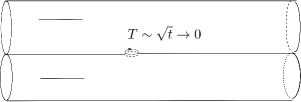
Figure 5: Light-cone diagram corresponding to a separating degeneration with $\alpha_{p_{1}}=0$.

• $N_{1}N_{2}=0$
  When $N_{2}=0$ for example, (3.2) and (3.3) become

  $$\partial\rho_{t}(x_{1}) \sim \partial\rho^{(1)}(x_{1})+\cdots\,,$$

  $$\partial\rho_{t}(x_{2}) \sim -t\partial_{p_{2}}\partial_{x_{2}}\ln E_{2}(x_{2},p_{2})\partial\rho^{(1)}(p_{1})+\cdots\,.$$ (3.7)

  Therefore $M_{2}/\sqrt{\left|t\right|}U_{2}$ corresponds to a tiny region in the light-cone diagram corresponding to $M_{t}$, which shrinks to a point in the limit $t\to 0$ and the collapsing neck has the coordinate size of order $t$ on the light-cone diagram. An example of such a situation is shown in Fig. 6. $\partial\rho^{(1)}(p_{1})=0$ in this case can be regarded as the situation in which some of the interaction points on $M_{1}$ come close to $p_{1}$.

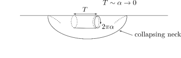
Figure 6: Light-cone diagram corresponding to a separating degeneration with $N_{2}=0$.

3.1.2 $g_{1}g_{2}=0$

The case where $g_{1}$ or $g_{2}$ vanish corresponds to the situation in which some of the punctures $Z_{1},\cdots,Z_{N}$ come close to each other. Let us consider the separating degeneration in which a Riemann surface $M$ degenerates into two surfaces $M_{1}$ and $M_{2}$ with genera $g_{1},g_{2}=0$ respectively. We assume that the punctures $Z_{1},\cdots,Z_{N_{1}}$ belong to $M_{1}$ and $Z_{N_{1}+1},\cdots,Z_{N}$ belong to $M_{2}$. Such a degeneration can be described as follows. Choose a point $p\in M$ and a neighborhood $U$ of $p$ such that the punctures $Z_{N_{1}+1},\cdots,Z_{N}$ are included in $U$. Let $D$ be the unit disk in $\mathbb{C}$ and define $z_{1}:U\to D$ to be the coordinate of $U$ such that $z_{1}(p)=0$. We take

$$z_{1}(Z_{r_{2}})=tz_{r_{2}}\,(r_{2}=N_{1}+1,\cdots,N)\,,$$

and consider the limit $t\to 0$ with $z_{r_{2}}$ fixed. When $\left|t\right|\ll 1$, $\rho(x_{1})$ for $x_{1}\in M/\sqrt{\left|t\right|}U$ becomes

$$\rho(x_{1}) \sim \sum_{r_{1}=1}^{N_{1}}\alpha_{r_{1}}\ln E(x_{1},Z_{r_{1}})+\alpha_{p_{1}}\ln E(x_{1},p_{1})$$

$$\quad-2\pi i\int_{P_{0}}^{x_{1}}\omega\frac{1}{\mathop{\mathrm{Im}}\Omega}\mathop{\mathrm{Im}}\left(\sum_{r_{1}=1}^{N_{1}}\alpha_{r_{1}}\int_{P_{0}}^{Z_{r_{1}}}\omega^{(1)}+\alpha_{p_{1}}\int_{P_{0}}^{p_{1}}\omega^{(1)}\right)$$

$$\equiv \rho^{(1)}(x_{1})\,.$$

For $x_{2}\in U$ such that $z_{1}(x_{2})=\mathcal{O}(\left|t\right|)$, defining $z_{2}\equiv\frac{z_{1}(x_{2})}{t}$,

$$\rho(x_{2}) \sim \rho^{(2)}(z_{2})-\frac{\alpha_{p_{2}}}{2}\ln t+\lim_{x\to p_{1}}(\rho^{(1)}(x)-\alpha_{p_{1}}\ln(x-p_{1}))\,,$$

$$\rho^{(2)}(z_{2}) = \sum_{r_{2}=N_{1}+1}^{N}\alpha_{r_{2}}\ln(z_{2}-z_{r_{2}})\,,$$

where

$$\alpha_{p_{1}}=\sum_{r_{2}=N_{1}+1}^{N}\alpha_{r_{2}}=-\alpha_{p_{2}}=-\sum_{r_{1}=1}^{N_{1}}\alpha_{r_{1}}\,.$$

If $\alpha_{p_{1}}\neq 0$, these formulas suggest that the limit corresponds to the one in which the length of an internal line with circumference $2\pi\alpha_{p_{1}}$ becomes infinite in the light-cone diagram. If $\alpha_{p_{1}}=0$, the collapsing neck can be described by a local coordinate $z\equiv\sqrt{t}z_{1}$ and

$$\rho(z)\sim\mbox{constant}+\sqrt{t}(c_{1}z+\frac{c_{2}}{z})\,,$$

where

$$c_{1} = \left.\partial\rho^{(1)}(z_{1})\right|_{z_{1}=0}\,,$$

$$c_{2} = \left.-z_{2}^{2}\partial\rho^{(2)}(z_{2})\right|_{z_{2}=\infty}\,.$$

Namely the light-cone diagrams are locally the same as those we encountered in the case where $g_{1},\,g_{2}$ are both positive.

3.2 Nonseparating degeneration

Next let us consider the nonseparating degeneration in which a Riemann surface of genus $g+1$ degenerates into a surface $M$ of genus $g$. The degeneration can be described by a model $M_{t}$ constructed as follows:

• Choose points $p_{1},p_{2}\in M$ and their disjoint neighborhoods $U_{1},U_{2}$. Let $z_{j}:U_{j}\to D$ be the coordinate of $U_{j}$ such that $z_{j}(p_{j})=0$.

• For $t\in D$, glue together the surfaces $M_{j}/\left|t\right|U_{j}\ (j=1,2)$ by the identification

  $$z_{1}z_{2}=t\,.$$

  The surface obtained is denoted by $M_{t}$. The degeneration limit corresponds to $t\to 0$.

The coordinate $\rho_{t}(z)$ on the light-cone diagram corresponding to $M_{t}$ is given by

$$\rho_{t}(z)=\sum_{r=1}^{N}\alpha_{r}\left[\ln E_{t}(z,Z_{r})-2\pi i\int_{P_{0}}^{z}\omega_{t}\frac{1}{\mathop{\mathrm{Im}}\Omega_{t}}\mathop{\mathrm{Im}}\int_{P_{0}}^{Z_{r}}\omega_{t}\right]\,.$$

Using the formulas given in [39, 40, 41, 42], it is straightforward to deduce that $\rho_{t}(z)$ can be expressed as

$$\rho_{t}(z) = \rho(z)$$ (3.8)

$$+\alpha_{p_{1}}\left[\ln E(z,p_{1})-2\pi i\int_{P_{0}}^{z}\omega\frac{1}{\mathop{\mathrm{Im}}\Omega}\mathop{\mathrm{Im}}\int_{P_{0}}^{p_{1}}\omega\right]$$

$$+\alpha_{p_{2}}\left[\ln E(z,p_{2})-2\pi i\int_{P_{0}}^{z}\omega\frac{1}{\mathop{\mathrm{Im}}\Omega}\mathop{\mathrm{Im}}\int_{P_{0}}^{p_{2}}\omega\right]\,,$$

$$+\mathrm{constant}+\mathcal{O}(t)\,,$$

for $\left|t\right|\ll 1$. Here

$$\rho(z)=\sum_{r=1}^{N}\alpha_{r}\left[\ln E(z,Z_{r})-2\pi i\int_{P_{0}}^{z}\omega\frac{1}{\mathop{\mathrm{Im}}\Omega}\mathop{\mathrm{Im}}\int_{P_{0}}^{Z_{r}}\omega\right]$$

gives the coordinate of the light-cone diagram corresponding to $M$ and

$$\alpha_{p_{2}}=-\alpha_{p_{1}}=\frac{1}{2\pi}\mathrm{Re}(\rho(p_{2})-\rho(p_{1}))\frac{1-\frac{2\pi}{\ln\left|t^{\prime}\right|}\mathop{\mathrm{Im}}\int_{p_{1}}^{p_{2}}\omega\frac{1}{\mathop{\mathrm{Im}}\Omega}\mathop{\mathrm{Im}}\int_{p_{1}}^{p_{2}}\omega}{-\frac{\ln\left|t^{\prime}\right|}{2\pi}+\frac{2\pi}{\ln\left|t^{\prime}\right|}\left(\mathop{\mathrm{Im}}\int_{p_{1}}^{p_{2}}\omega\frac{1}{\mathop{\mathrm{Im}}\Omega}\mathop{\mathrm{Im}}\int_{p_{1}}^{p_{2}}\omega\right)^{2}}\,,$$

with

$$t^{\prime}=\frac{t}{E(p_{1},p_{2})E(p_{2},p_{1})}\,.$$

Using (3.8), we can classify the light-cone diagrams corresponding to the nonseparating degeneration according to the value of $\mathrm{Re}(\rho(p_{2})-\rho(p_{1}))$ as follows:

• $\mathrm{Re}(\rho(p_{2})-\rho(p_{1}))\neq 0$
  If $\mathrm{Re}(\rho(p_{2})-\rho(p_{1}))\neq 0$, we can see from (3.8) that this kind of degeneration corresponds to a limit of light-cone diagram in which the circumference of an internal line tends to zero as depicted in Fig. 7.

Figure 7: Nonseparating degeneration with $\mathrm{Re}(\rho(p_{2})-\rho(p_{1}))\neq 0$.

• $\mathrm{Re}(\rho(p_{2})-\rho(p_{1}))=0$
  When $\mathrm{Re}(\rho(p_{2})-\rho(p_{1}))=0$, $\rho_{t}(x)$ becomes

  $$\rho_{t}(x)=\rho(x)+t\left[\partial_{p_{1}}\ln E(x,p_{1})\partial\rho(p_{2})+\partial_{p_{2}}\ln E(x,p_{2})\partial\rho(p_{1})\right]+\cdots\,.$$

  Therefore, for $x\sim p_{1}$

  $$\rho_{t}(x)=\mbox{constant}+c_{1}z_{1}+\frac{c_{2}t}{z_{1}}+\cdots\,,$$ (3.9)

  where $z_{1}=z_{1}(x)$ and

  $$c_{1} = \left.\partial\rho(z_{1})\right|_{z_{1}=0}\,,$$

  $$c_{2} = \left.\partial\rho(z_{2})\right|_{z_{2}=0}\,.$$

  Similarly, for $x\sim p_{2}$

  $$\rho_{t}(x)=\mbox{constant}+c_{2}z_{2}+\frac{c_{1}t}{z_{2}}+\cdots\,,$$ (3.10)

  where $z_{2}=z_{2}(x)$. Hence the $\rho_{t}$ has the same expression as those in (3.4), (3.5). When $c_{1}c_{2}\neq 0$, the degeneration of this type can be represented by the light-cone diagrams depicted in Figs. 8 and 9. There are two interaction points in the light-cone diagram corresponding to $M_{t}$ which come close to each other and the surface develops a narrow neck in the limit $t\to 0$. They are included in a region which has coordinate size of order $\sqrt{t}$ on the light-cone diagram and shrinks to a point in the limit $t\to 0$. $c_{1}c_{2}=0$ corresponds to the case in which some interaction points on $M$ come close to $p_{1}$ or $p_{2}$.

Figure 8: An example of nonseparating degeneration with $\mathrm{Re}(\rho(p_{2})-\rho(p_{1}))=0$.

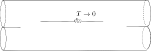
Figure 9: Another example of nonseparating degeneration with $\mathrm{Re}(\rho(p_{2})-\rho(p_{1}))=0$.

3.3 Combined limits

In the discussions above, we have implicitly assumed that the parameters $\alpha_{p_{1}}=\sum\alpha_{r_{2}}$ or $\mathrm{Re}(\rho(p_{2})-\rho(p_{1}))$ are fixed in taking the degeneration limit $t\to 0$. This is true if the degeneration considered is the only one which occurs on the surface. If we consider the situation where several degenerations happen simultaneously, these parameters are not necessarily fixed and we encounter new classes of light-cone diagrams corresponding to degeneration.

Figure 10: A combination of degeneration limits.

Taking such situations into account, the light-cone diagram in the degeneration limits are classified by the behavior of the parameter $\alpha_{p_{1}}=-\alpha_{p_{2}}$ in the limit $t\to 0$. For $z_{1},z_{2}\ll 1,\,t\ll 1$, we have

$$\partial\rho_{t}(z_{1}) \sim \frac{\alpha_{p_{1}}}{z_{1}}+\mbox{higher order terms in }t\,,$$

$$\partial\rho_{t}(z_{2}) \sim \frac{\alpha_{p_{2}}}{z_{2}}+\mbox{higher order terms in }t\,,$$

irrespective of whether the degeneration is separating or nonseparating. If $\alpha_{p_{1}}$tends to a finite nonvanishing value in the limit $t\to 0$, these imply that the light-cone diagram develops an infinitely long cylinder with finite width. The diagrams depicted in Figs. 4, 10 are in this class. If $\alpha_{p_{1}}$tends to $0$ as $t\to 0$, the light-cone diagram develops a cylinder with vanishing width, provided $\frac{\alpha_{p_{1}}}{z_{1}},\frac{\alpha_{p_{2}}}{z_{2}}$ dominate the higher order terms in $t$. For example, if $\partial\rho_{1}(p_{1})\partial\rho_{2}(p_{2})\neq 0$, defining $z=t^{\frac{1}{2}}z_{1}$ as in (3.6), we have

$$\rho_{t}(z)\sim\alpha_{p_{1}}\ln z+t^{\frac{1}{2}}(c_{1}z+\frac{c_{2}}{z})+\cdots\,.$$ (3.11)

Therefore if $\alpha_{p_{1}}$ goes to $0$ slower than $t^{\frac{1}{2}}$ in the limit $t\to 0$, the surface develops a cylinder with vanishing width. If $t^{-\frac{1}{2}}\alpha_{p_{1}}$ tends to a finite value in the limit $t\to 0$, we have

$$\rho_{t}(z)\sim t^{\frac{1}{2}}(c_{1}z+\frac{c_{2}}{z}+\alpha\ln z)+\mbox{constant}\,,$$

where $\alpha=\lim_{t\to 0}t^{-\frac{1}{2}}\alpha_{p_{1}}$. The degeneration of this type can be represented by the light-cone diagrams depicted in Figs. 5, 8, 9, but this time

$$\oint_{\mbox{neck}}dz\partial\rho_{t}\sim 2\pi it^{\frac{1}{2}}\alpha\neq 0\,,$$

namely the coordinate $\rho$ can be multivalued around the neck. If $\alpha_{p_{1}}$ goes to $0$ faster than $t^{\frac{1}{2}}$, the first term in (3.11) can be ignored and we have $\rho$ single-valued around the neck. $\partial\rho_{1}(p_{1})\partial\rho_{2}(p_{2})=0$ case corresponds to the situation in which some interaction points come close to $p_{1},\,p_{2}$.

3.4 Classification of the light-cone diagrams in the degeneration limits

To summarize, what happens to a light-cone diagram in the degeneration limit can be classified by the behavior of the degenerating cycle as follows:

1. The light-cone diagram develops an infinitely long cylinder with nonvanishing width.
   The diagrams presented in Figs. 4, 10 belong to this class.

2. The light-cone diagram develops an infinitely thin cylinder.
   The diagram depicted in Fig. 7 belongs to this class.

3. The light-cone diagram develops a narrow neck included in a region which shrinks to a point.
   The diagrams shown in Figs. 5, 6, 8, 9 belong to this class.

A diagram of the first type includes a long cylinder and can definitely be considered as corresponding to the infrared region of the integration over the moduli space. The divergent contributions from such diagrams can be made finite by the Feynman $i\varepsilon$ as will be shown in the next section. On the other hand, that of the third type appears to correspond to the ultraviolet region with respect to the world sheet metric $ds^{2}=d\rho d\bar{\rho}$, although the collapsing neck is conformally equivalent to a long cylinder. We need to introduce a linear dilaton background to regularize the divergences coming from the diagrams in this category and the Feynman $i\varepsilon$ plays no roles in this case. The second type is something in between and we need both $i\varepsilon$ and a linear dilaton background to deal with the divergence coming from such a configuration.

4 Divergences of the amplitudes

Divergences of the amplitudes arise from the diagrams in which degenerations and/or collisions of interaction points occur. In this section, we examine the divergences of the amplitude (2.13) corresponding to these configurations.

4.1 Diagrams which involve cylinders with infinite length and nonvanishing width

Let us first consider the first type of degeneration limit in the classification in subsection 3.4, in which the diagram develops a cylinder with height $T\to\infty$ and nonvanishing circumference. In the light-cone gauge perturbation theory, such cylinders appear as follows. Let us order the interaction points $z_{I}\,(I=1,\ldots,2g-2+N)$ so that

$$\mathrm{Re}\rho(z_{1})\leq\mathrm{Re}\rho(z_{2})\leq\cdots\leq\mathrm{Re}\rho(z_{2g-2+N})\,,$$

and define the moduli parameters corresponding to the heights as

$$T_{I}\equiv\mathrm{Re}\rho(z_{I+1})-\mathrm{Re}\rho(z_{I})\,(I=1,\ldots,2g-3+N)\,.$$

Long cylinders appear in the limit $T_{I}\to\infty$. In studying the divergence from this region of the moduli space, the relevant part of the amplitude is of the form

$$\int_{0}^{\infty}dT_{I}\exp\left[-T_{I}\left(\sum_{j}\frac{L_{0}^{(j)}+\bar{L}_{0}^{(j)}-1+Q^{2}-i\varepsilon}{\alpha_{j}}-\sideset{}{{}^{\prime}}{\sum}_{r}p_{r}^{-}\right)\right]\,,$$ (4.1)

where $j$ labels the cylinders which include the region $\mathrm{Re}\rho(z_{I})\leq\mathrm{Re}\rho\leq\mathrm{Re}\rho(z_{I+1})$ (see Fig. 11) and $\alpha_{j},\,L_{0}^{(j)},\,\bar{L}_{0}^{(j)}$ denote the $\alpha,\,L_{0},\,\bar{L}_{0}$ defined on the $j$-th cylinder respectively. $r$ labels the external lines and $\sum^{\prime}$ denotes the sum over those with $p_{r}^{-}>0$. The degeneration limit corresponds to the one in which $T_{I}$ goes to infinity. Since the lowest eigenvalue of $L_{0}^{(j)}+\bar{L}_{0}^{(j)}$ is $1-Q^{2}$ for the GSO even sector, the integral (4.1) could diverge because of the contribution from the limit.

The divergence coming from this kind of degeneration can be dealt with by deforming the contour of integration over $T_{I}$ [43, 44, 45]. As is suggested in [43], we take the contour to be as

$$\left(\int_{0}^{T_{0}}+\int_{T_{0}}^{T_{0}+i\infty}\right)dT_{I}\,,$$ (4.2)

with $T_{0}\gg 1$. Since

$$\left|\exp\left[-(T_{0}+ia)\left(\sum_{j}\frac{L_{0}^{(j)}+\bar{L}_{0}^{(j)}-1+Q^{2}-i\varepsilon}{\alpha_{j}}-\sideset{}{{}^{\prime}}{\sum}_{r}p_{r}^{-}\right)\right]\right|$$

$$\qquad=\left|\exp\left[-T_{0}\left(\sum_{j}\frac{L_{0}^{(j)}+\bar{L}_{0}^{(j)}-1+Q^{2}-i\varepsilon}{\alpha_{j}}-\sideset{}{{}^{\prime}}{\sum}_{r}p_{r}^{-}\right)\right]\right|\exp\left(-a\varepsilon\sum_{j}\frac{1}{\alpha_{j}}\right)\,,$$

the second integral in (4.2) yields a finite result for $\varepsilon>0$. Thus the integral over $T_{I}$ is essentially cut off at $T_{I}=T_{0}$ and the degeneration becomes harmless.

Figure 11: Cylinders in a light-cone diagram.

In order to get the amplitudes, we need to take the limit $\varepsilon\to 0$. Notice that the divergences associated with the tadpole graphs correspond to the separating degeneration with $N_{1}N_{2}=0$ described in subsection 3.1.1. As we will see in the following subsections, they are regularized by taking $Q^{2}$ large enough and the Feynman $i\varepsilon$ is irrelevant. The modified momentum conservation law of $p^{1}$ for $g$-loop two point function is given by

$$p_{1}^{1}+p_{2}^{1}+2Q(1-g)=0\,.$$

Therefore if $p_{1}^{\mu}$ is on-shell, $p_{2}^{\mu}$ is generically off-shell, for $g\neq 0$. This implies that the divergences associated with mass renormalization are also regularized by taking $Q\neq 0$. Therefore the procedures given in [46, 47, 48, 49] shall be relevant in taking the limit $Q\to 0$ rather than $\varepsilon\to 0$. Possible divergences in the limit $\varepsilon\to 0$ can be analyzed as in the usual field theory and we expect that they cancel each other if one calculates physical quantities.

4.2 Singular behavior of $F_{N}^{(g)}$

Since the first type of degeneration in the classification in subsection 3.4 is taken care of, what we should grapple with are other types of singularities, namely the degenerations of types 2 and 3 and the collisions of interaction points. The integration variables in the expression (2.13) are given by differences of the coordinates $\rho,\bar{\rho}$ of the interaction points and magnitudes of jump discontinuities of $\rho,\bar{\rho}$. Let $x^{j}\in\mathbb{R}\,(j=1,\cdots,n)$ denote these integration variables. The calculation of the amplitude boils down to that of an integral

$$\int d^{n}xF_{N}^{(g)}(\vec{x})\,,$$ (4.3)

where $F_{N}^{(g)}(\vec{x})$ denotes the $F_{N}^{(g)}$ as a function of the variables $x^{1},\cdots,x^{n}$. The singularities we are dealing with occur when interaction points collide and/or cylinders become infinitely thin. Therefore a necessary and sufficient condition for $\vec{x}$ to correspond to such singularities can be expressed as

$$\vec{v}_{k}\cdot\vec{x}=0\,,$$ (4.4)

for some $\vec{v}_{k}\in\mathbb{R}^{n}\,(k=1,\cdots)$. In order to study the behavior of $F_{N}^{(g)}(\vec{x})$ at these singularities, it is convenient to express $F_{N}^{(g)}(\vec{x})$ as

$$F_{N}^{(g)}(\vec{x})=e^{-\frac{1-Q^{2}}{2}\Gamma\left[\sigma;g_{z\bar{z}}^{\mathrm{A}}\right]}\left\langle\mathcal{O}_{N}^{(g)}\right\rangle\,,$$

where

$$\left\langle\mathcal{O}\right\rangle \equiv \int\left[dX^{i}d\psi^{i}d\bar{\psi}^{i}\right]_{g_{z\bar{z}}^{\mathrm{A}}}e^{-S\left[X^{i},\psi^{i},\bar{\psi}^{i};g_{z\bar{z}}^{\mathrm{A}}\right]}\mathcal{O}\,,$$

$$\mathcal{O}_{N}^{(g)} \equiv \prod_{I=1}^{2g-2+N}\left(\left|\partial^{2}\rho\left(z_{I}\right)\right|^{-\frac{3}{2}}T_{F}^{\mathrm{LC}}\left(z_{I}\right)\bar{T}_{F}^{\mathrm{LC}}\left(\bar{z}_{I}\right)\right)\prod_{r=1}^{N}V_{r}^{\mathrm{LC}}\,.$$

The integrals over the lengths of cylinders are essentially cut off by taking $\varepsilon>0$. Therefore we should worry about the singularity of $F_{N}^{(g)}(\vec{x})$ at finite values of the coordinates $x^{j}$. Such singularities can be studied by calculating the derivatives of $F_{N}^{(g)}(\vec{x})$ with respect to $x^{1},\cdots,x^{n}$, which can be expressed by contour integrals of the correlation functions with energy-momentum tensor insertions:

$$e^{-\frac{1-Q^{2}}{2}\Gamma\left[\sigma;g_{z\bar{z}}^{\mathrm{A}}\right]}\left\langle T(\rho)\mathcal{O}_{N}^{(g)}\right\rangle,\,e^{-\frac{1-Q^{2}}{2}\Gamma\left[\sigma;g_{z\bar{z}}^{\mathrm{A}}\right]}\left\langle\bar{T}(\bar{\rho})\mathcal{O}_{N}^{(g)}\right\rangle\,.$$

As we will see in the following, these correlation functions become singular when $\rho,\bar{\rho}$ coincide with those of the interaction points. Therefore the contour integrals diverge when the interaction points pinch the contour. This is exactly what happens in the situations we are dealing with. Away from the singularities, $F_{N}^{(g)}(\vec{x})$ is a differentiable function of the parameters $x^{j}$.

4.2.1 Singular behavior of $F_{N}^{(g)}(\vec{x})$ associated with the configuration depicted in Fig. 6

As an example, let us study the singular behavior of $F_{N}^{(g)}(\vec{x})$ in the limit illustrated in Fig. 6. We here consider the situation where the tiny cylinder is embedded in a light-cone diagram as depicted in Fig. 12.

We would like to calculate the variation of $F_{N}^{(g)}(\vec{x})$ under a change of the shape of the tiny cylinder fixing the other part of the diagram. Such a change corresponds to a change of the moduli parameters and it induces a variation

$$\rho(z)\to\rho(z)+\delta\rho(z)\,,$$

of the function $\rho(z)$ in (2.12). The change is parametrized by the variation of the circumference of the cylinder, i.e. $2\pi\delta\alpha$, and $\delta\mathcal{T}_{1},\delta\mathcal{T}_{2}$ defined by

$$\delta\mathcal{T}_{1} = \int_{C_{1}}dz^{\prime}\partial\delta\rho(z^{\prime})\,,$$

$$\delta\mathcal{T}_{2} = \int_{C_{2}}dz^{\prime}\partial\delta\rho(z^{\prime})\,,$$

where the contours $C_{1},C_{2}$ are those shown in Fig. 13. $\delta\alpha$ can also be expressed as

$$\delta\alpha=\oint_{C_{T1}}\frac{dz}{2\pi i}\partial\delta\rho(z)=-\oint_{C_{T2}}\frac{dz}{2\pi i}\partial\delta\rho(z)\,,$$

where the contours $C_{T1},C_{T2}$ are those depicted in Fig. 14.

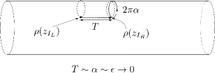
Figure 12: Fig. 6 embedded in a light-cone diagram.

Figure 13: Contours $C_{1},C_{2}$.

Figure 14: Contours $C_{T1},C_{T2},C_{\alpha},C_{R},C_{L}$.

$\delta F_{N}^{(g)}(\vec{x})$ is given by

$$\delta F_{N}^{(g)}(\vec{x}) = -\delta\mathcal{T}_{1}\oint_{C_{T1}}\frac{d\rho}{2\pi i}\left\langle T(\rho)\mathcal{O}_{N}^{(g)}\right\rangle e^{-\frac{1-Q^{2}}{2}\Gamma}-\delta\mathcal{T}_{2}\oint_{C_{T2}}\frac{d\rho}{2\pi i}\left\langle T(\rho)\mathcal{O}_{N}^{(g)}\right\rangle e^{-\frac{1-Q^{2}}{2}\Gamma}$$ (4.5)

$$+2\pi i\delta\alpha\oint_{C_{\alpha}}\frac{d\rho}{2\pi i}\left\langle T(\rho)\mathcal{O}_{N}^{(g)}\right\rangle e^{-\frac{1-Q^{2}}{2}\Gamma}$$

$$\quad+\mathrm{c.c.}\,,$$

where the contours $C_{T1},C_{T2},C_{\alpha}$ are those indicated in Fig. 14. By using the transformation formula

$$T(\rho) = \frac{1}{(\partial\rho(z))^{2}}\left(T(z)-(1-Q^{2})\left\{\rho,z\right\}\right)\,,$$

$$\left\{\rho,z\right\} = \frac{\partial^{3}\rho}{\partial\rho}-\frac{3}{2}\left(\frac{\partial^{2}\rho}{\partial\rho}\right)^{2}\,,$$

contour integrals of the energy-momentum tensor are expressed as

$$\oint_{C}\frac{d\rho}{2\pi i}T(\rho) = \oint_{C}\frac{dz}{2\pi i}\frac{1}{\partial\rho(z)}\left(T(z)-(1-Q^{2})\left\{\rho,z\right\}\right)\,,$$

$$\oint_{\bar{C}}\frac{d\bar{\rho}}{2\pi i}\bar{T}(\bar{\rho}) = \oint_{\bar{C}}\frac{d\bar{z}}{2\pi i}\frac{1}{\partial\bar{\rho}(\bar{z})}\left(\bar{T}(\bar{z})-(1-Q^{2})\left\{\bar{\rho},\bar{z}\right\}\right)\,.$$

Taking the local coordinates $z,\bar{z}$ convenient for calculation, one can evaluate the right hand side of (4.5).

Figure 15: Two pants and the paths $P_{L}\,(\mathrm{E}\to\mathrm{B}\to\mathrm{C}\to\mathrm{D}\to\mathrm{D}\to\mathrm{C}\to\mathrm{B}\to\mathrm{E})$ and $P_{R}\,(\mathrm{A}\to\mathrm{B}\to\mathrm{C}\to\mathrm{D}\to\mathrm{D}\to\mathrm{C}\to\mathrm{B}\to\mathrm{A})$.

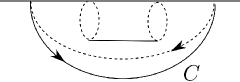
Figure 16: Contour $C$.

Decomposing the diagram into two pants and cutting them open as in Fig. 15, it is straightforward to show that the right hand side of (4.5) is equal to

$$\int_{P_{L}}\frac{dz}{2\pi i}\frac{\delta\rho(z)-\delta\rho(z_{I_{L}})}{\partial\rho(z)}\left\langle\left(T(z)-(1-Q^{2})\left\{\rho,z\right\}\right)\mathcal{O}_{N}^{(g)}\right\rangle e^{-\frac{1-Q^{2}}{2}\Gamma}$$

$$+\int_{P_{R}}\frac{dz}{2\pi i}\frac{\delta\rho(z)-\delta\rho(z_{I_{R}})}{\partial\rho(z)}\left\langle\left(T(z)-(1-Q^{2})\left\{\rho,z\right\}\right)\mathcal{O}_{N}^{(g)}\right\rangle e^{-\frac{1-Q^{2}}{2}\Gamma}$$

$$\quad+\mathrm{c.c.}\,.$$ (4.6)

$P_{L},P_{R}$ are the paths depicted in Fig. 15. $\delta\rho(z)-\delta\rho(z_{I_{L}})$ and $\delta\rho(z)-\delta\rho(z_{I_{R}})$ are defined as

$$\delta\rho(z)-\delta\rho(z_{I_{L}}) = \int_{z_{I_{L}}}^{z}dz^{\prime}\partial\delta\rho(z^{\prime})\,,$$

$$\delta\rho(z)-\delta\rho(z_{I_{R}}) = \int_{z_{I_{R}}}^{z}dz^{\prime}\partial\delta\rho(z^{\prime})\,,$$ (4.7)

where the paths of integration are taken to be within the regions $U_{L}$ and $U_{R}$ in Fig. 15 respectively. Deforming the contours, we can show

$$\delta F_{N}^{(g)}(\vec{x}) = -\oint_{z_{I_{L}}}\frac{dz}{2\pi i}\frac{\delta\rho(z)-\delta\rho(z_{I_{L}})}{\partial\rho(z)}\left\langle\left(T(z)-(1-Q^{2})\left\{\rho,z\right\}\right)\mathcal{O}_{N}^{(g)}\right\rangle e^{-\frac{1-Q^{2}}{2}\Gamma}$$ (4.8)

$$-\oint_{z_{I_{R}}}\frac{dz}{2\pi i}\frac{\delta\rho(z)-\delta\rho(z_{I_{R}})}{\partial\rho(z)}\left\langle\left(T(z)-(1-Q^{2})\left\{\rho,z\right\}\right)\mathcal{O}_{N}^{(g)}\right\rangle e^{-\frac{1-Q^{2}}{2}\Gamma}$$

$$+\oint_{C}\frac{dz}{2\pi i}\frac{\delta\rho(z)-\delta\rho(z_{I_{L}})}{\partial\rho(z)}\left\langle\left(T(z)-(1-Q^{2})\left\{\rho,z\right\}\right)\mathcal{O}_{N}^{(g)}\right\rangle e^{-\frac{1-Q^{2}}{2}\Gamma}$$

$$-\delta\mathcal{T}_{2}\oint_{C_{R}}\frac{dz}{2\pi i}\frac{1}{\partial\rho(z)}\left\langle\left(T(z)-(1-Q^{2})\left\{\rho,z\right\}\right)\mathcal{O}_{N}^{(g)}\right\rangle e^{-\frac{1-Q^{2}}{2}\Gamma}$$

$$\quad+\mathrm{c.c.}\,,$$

where $C$ is the contour surrounding the tiny cylinder depicted in Fig. 16.

In this expression, the right hand side can be evaluated once we know the behaviors of $\rho(z),T(z)$ near the cylinder. Taking a good local coordinate $z$ around the cylinder, the coordinate $\rho(z)$ of the light-cone diagram shall be expressed as

$$\rho(z)=\epsilon\tilde{\rho}(z)+\mbox{constant}\,,$$

and the limit to be considered is $\epsilon\to 0$. In order to get the singular behavior of $F_{N}^{(g)}(\vec{x})$ in the limit $\epsilon\to 0$, we consider the variation $\delta F_{N}^{(g)}(\vec{x})$ under $\epsilon\to\epsilon+\delta\epsilon$. For $\epsilon\ll 1$ and $z$ close to an interaction point $z_{I}$,

$$\delta\rho(z)-\delta\rho(z_{I}) \sim \frac{\delta\epsilon}{2}\partial^{2}\tilde{\rho}(z_{I})(z-z_{I})^{2}\,,$$

$$\partial\rho(z) \sim \epsilon\partial^{2}\tilde{\rho}(z_{I})(z-z_{I})\,,$$

$$T(z)\mathcal{O}_{N}^{(g)} \sim \left(\frac{\frac{3}{2}}{(z-z_{I})^{2}}+\cdots\right)\mathcal{O}_{N}^{(g)}\,,$$

$$\left\{\rho,z\right\} \sim \frac{-\frac{3}{2}}{(z-z_{I})^{2}}+\cdots\,,$$

and

$$-\oint_{z_{I}}\frac{dz}{2\pi i}\frac{\delta\rho(z)-\delta\rho(z_{I})}{\partial\rho(z)}\left\langle\left(T(z)-(1-Q^{2})\left\{\rho,z\right\}\right)\mathcal{O}_{N}^{(g)}\right\rangle e^{-\frac{1-Q^{2}}{2}\Gamma}\sim-\frac{3}{4}(2-Q^{2})\frac{\delta\epsilon}{\epsilon}F_{N}^{(g)}(\vec{x})\,.$$ (4.9)

(3.7) implies that $\tilde{\rho}(z)$ has a simple pole at the degenerating puncture and $C$ is a contour around it. Using these facts, we obtain

$$\oint_{C}\frac{dz}{2\pi i}\frac{\delta\rho(z)-\delta\rho(z_{I_{L}})}{\partial\rho(z)}\left\langle\left(T(z)-(1-Q^{2})\left\{\rho,z\right\}\right)\mathcal{O}_{N}^{(g)}\right\rangle e^{-\frac{1-Q^{2}}{2}\Gamma}$$

$$\quad\sim\frac{\delta\epsilon}{\epsilon}\oint_{C}\frac{dz}{2\pi i}z\left\langle T(z)\mathcal{O}_{N}^{(g)}\right\rangle e^{-\frac{1-Q^{2}}{2}\Gamma}$$

$$\quad\sim 0\,,$$ (4.10)

because the momentum flowing through the collapsing neck is $0$. The fourth term on the right hand side of (4.8) is of order $\delta\epsilon$. Therefore we get

$$\delta F_{N}^{(g)}(\vec{x})\sim\left(-6+3Q^{2}\right)\frac{\delta\epsilon}{\epsilon}F_{N}^{(g)}(\vec{x})\,,$$

from which we can deduce that $F_{N}^{(g)}(\vec{x})$ is expressed as

$$F_{N}^{(g)}(\vec{x})\sim\epsilon^{-6+3Q^{2}}\times\mathrm{constant}\,,$$ (4.11)

for $\epsilon\sim 0$.

In general, the behavior of $F_{N}^{(g)}(\vec{x})$ in the limit where subregions of the diagram shrink to points can be studied in the same way. The variation $\delta F_{N}^{(g)}$ under a change of the shape of the diagram can be expressed as a sum of contour integrals of correlation functions with energy-momentum tensor insertions. Decomposing the diagram into pants, expressing the integrals in terms of those around the pants and deforming the contours of the integrations, $\delta F_{N}^{(g)}(\vec{x})$ can be expressed by contour integrals in the shrinking subregions. It is possible to evaluate them taking coordinates convenient for describing those regions and deduce the singular behavior of $F_{N}^{(g)}(\vec{x})$ in the limit.

4.2.2 Singular behavior of $F_{N}^{(g)}(\vec{x})$ associated with the configuration depicted in Fig. 7

As another example, let us consider the degeneration in which the light-cone diagram develops a cylinder with vanishing width. Suppose that the cylinder is embedded in the diagram as illustrated in Fig. 17. We take the limit $\alpha\to 0$ with $T$ fixed.

In order to get the singular behavior of $F_{N}^{(g)}(\vec{x})$ in the limit $\alpha\to 0$, we evaluate the variation of $F_{N}^{(g)}$ under $\alpha\to\alpha+\delta\alpha$ which is given by

$$\delta F_{N}^{(g)}(\vec{x})=2\pi i\delta\alpha\oint_{C_{\alpha}}\frac{dz}{2\pi i}\frac{1}{\partial\rho(z)}\left\langle\left(T(z)-(1-Q^{2})\left\{\rho,z\right\}\right)\mathcal{O}_{N}^{(g)}\right\rangle e^{-\frac{1-Q^{2}}{2}\Gamma}+\mathrm{c.c.}\,,$$ (4.12)

where the contour $C_{\alpha}$ is shown in Fig. 18. $C_{\alpha}$ either closes or ends in punctures. We decompose the relevant part of the diagram into two pants which are the regions bounded by the curves $C_{L1},C_{L2},C_{T}$ and $C_{R1},C_{R2},C_{T}$ respectively and a cylindrical region bounded by $C_{L2},C_{R2}$ in Fig. 18. We also introduce a local coordinate $z_{L}$ around the interaction point $\rho(z_{I_{L}})$ such that

$$\rho(z_{L})\sim\alpha(z_{L}-1-\ln z_{L})+\rho(z_{I_{L}})\,,$$

and similarly $z_{R}$ around $\rho(z_{I_{R}})$ such that

$$\rho(z_{R})\sim\alpha(-z_{R}+1+\ln z_{R})+\rho(z_{I_{R}})\,,$$

for $\alpha\ll 1$. We take the contour $C_{T}$ to be along the curve

$$\left|z_{L}\right| \sim \exp\left(-\frac{T_{L}}{\alpha}-1\right)\,,$$

$$\left|z_{R}\right| \sim \exp\left(-\frac{T_{R}}{\alpha}-1\right)\,,$$

with

$$T_{L}+T_{R}=T\,.$$

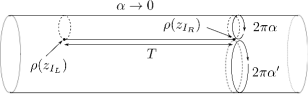
Figure 17: Fig. 7 embedded in a light-cone diagram.

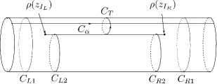
Figure 18: Contours.

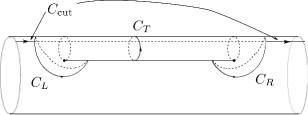
Figure 19: Contours $C_{L},C_{R},C_{\mathrm{cut}}$.

Proceeding as in (4.6), (4.8), we get

$$\delta F_{N}^{(g)}(\vec{x}) = -\oint_{1}\frac{dz_{L}}{2\pi i}\frac{\delta\rho(z_{L})-\delta\rho(z_{I_{L}})}{\partial\rho(z_{L})}\left\langle\left(T(z)-(1-Q^{2})\left\{\rho,z\right\}\right)\mathcal{O}_{N}^{(g)}\right\rangle e^{-\frac{1-Q^{2}}{2}\Gamma}$$ (4.13)

$$+\int_{C_{T}}\frac{dz_{L}}{2\pi i}\frac{\delta\rho(z_{L})-\delta\rho(z_{I_{L}})}{\partial\rho(z_{L})}\left\langle\left(T(z)-(1-Q^{2})\left\{\rho,z\right\}\right)\mathcal{O}_{N}^{(g)}\right\rangle e^{-\frac{1-Q^{2}}{2}\Gamma}$$

$$+\int_{C_{L}}\frac{dz_{L}}{2\pi i}\frac{\delta\rho(z_{L})-\delta\rho(z_{I_{L}})}{\partial\rho(z_{L})}\left\langle\left(T(z)-(1-Q^{2})\left\{\rho,z\right\}\right)\mathcal{O}_{N}^{(g)}\right\rangle e^{-\frac{1-Q^{2}}{2}\Gamma}$$

$$-\oint_{1}\frac{dz_{R}}{2\pi i}\frac{\delta\rho(z_{R})-\delta\rho(z_{I_{R}})}{\partial\rho(z_{R})}\left\langle\left(T(z)-(1-Q^{2})\left\{\rho,z\right\}\right)\mathcal{O}_{N}^{(g)}\right\rangle e^{-\frac{1-Q^{2}}{2}\Gamma}$$

$$-\int_{C_{T}}\frac{dz_{R}}{2\pi i}\frac{\delta\rho(z_{R})-\delta\rho(z_{I_{R}})}{\partial\rho(z_{R})}\left\langle\left(T(z)-(1-Q^{2})\left\{\rho,z\right\}\right)\mathcal{O}_{N}^{(g)}\right\rangle e^{-\frac{1-Q^{2}}{2}\Gamma}$$

$$+\int_{C_{R}}\frac{dz_{R}}{2\pi i}\frac{\delta\rho(z_{R})-\delta\rho(z_{I_{R}})}{\partial\rho(z_{R})}\left\langle\left(T(z)-(1-Q^{2})\left\{\rho,z\right\}\right)\mathcal{O}_{N}^{(g)}\right\rangle e^{-\frac{1-Q^{2}}{2}\Gamma}$$

$$+2\pi i\delta\alpha\oint_{C_{\mathrm{cut}}}\frac{dz}{2\pi i}\frac{1}{\partial\rho(z)}\left\langle\left(T(z)-(1-Q^{2})\left\{\rho,z\right\}\right)\mathcal{O}_{N}^{(g)}\right\rangle e^{-\frac{1-Q^{2}}{2}\Gamma}$$

$$\quad+\mathrm{c.c.}\,,$$

where $C_{\mathrm{cut}}$ denotes parts of the contour $C_{\alpha}$ presented in Fig. 19, together with $C_{L},C_{R}$. The first term on the right hand side of (4.13) can be evaluated in the same way as (4.9) and we get

$$-\oint_{1}\frac{dz_{L}}{2\pi i}\frac{\delta\rho(z_{L})-\delta\rho(z_{I_{L}})}{\partial\rho(z_{L})}\left\langle\left(T(z)-(1-Q^{2})\left\{\rho,z\right\}\right)\mathcal{O}_{N}^{(g)}\right\rangle e^{-\frac{1-Q^{2}}{2}\Gamma}\sim-\frac{3}{4}(2-Q^{2})\frac{\delta\alpha}{\alpha}F_{N}^{(g)}\,.$$

The second term is evaluated to be

$$\int_{C_{T}}\frac{dz_{L}}{2\pi i}\frac{\delta\rho(z_{L})-\delta\rho(z_{I_{L}})}{\partial\rho(z_{L})}\left\langle\left(T(z)-(1-Q^{2})\left\{\rho,z\right\}\right)\mathcal{O}_{N}^{(g)}\right\rangle e^{-\frac{1-Q^{2}}{2}\Gamma}$$

$$\quad\sim-\int_{0}^{2\pi}\frac{d\sigma}{2\pi}\frac{\delta\alpha}{-\alpha}z_{L}^{{}^{2}}(\frac{T_{L}}{\alpha}-i\sigma)\frac{1}{z_{L}^{2}}\left\langle\left(\frac{1}{2}\left|\vec{p}\right|^{2}+Qp^{1}+\frac{1}{2}Q^{2}\right)\mathcal{O}_{N}^{(g)}\right\rangle e^{-\frac{1-Q^{2}}{2}\Gamma}$$

$$\quad\sim\frac{D}{4}\frac{\delta\alpha}{\alpha}+\mbox{imaginary part}\,,$$ (4.14)

where we have used the fact that the states propagating through $C_{T}$ are projected to be GSO even and the dominant contributions in the limit $\alpha\to 0$ come from the states with the momentum $p^{i}=-Q\delta_{i,1}$. $D$ denotes the number of noncompact bosons in the world sheet theory and $\frac{D}{4}\frac{\delta\alpha}{\alpha}$ in the last line originates from the momentum integral. For $\alpha\ll 1$, taking the contour $C_{L}$ to be along the curve $\left|z_{L}\right|=\alpha^{-\gamma}\,(0<\gamma<1)$, the third term on the right hand side of (4.13) is evaluated as

$$\int_{C_{L}}\frac{dz_{L}}{2\pi i}\frac{\delta\rho(z_{L})-\delta\rho(z_{I_{L}})}{\partial\rho(z_{L})}\left\langle\left(T(z)-(1-Q^{2})\left\{\rho,z\right\}\right)\mathcal{O}_{N}^{(g)}\right\rangle e^{-\frac{1-Q^{2}}{2}\Gamma}$$

$$\quad\sim\frac{\delta\alpha}{\alpha}\oint_{C_{L}}\frac{dz_{L}}{2\pi i}z_{L}\left\langle T(z)\mathcal{O}_{N}^{(g)}\right\rangle e^{-\frac{1-Q^{2}}{2}\Gamma}+\mathrm{constant}\times\delta(\alpha^{\gamma})$$

$$\quad\sim-\frac{1}{2}Q^{2}\frac{\delta\alpha}{\alpha}F_{N}^{(g)}\,,$$ (4.15)

where we have ignored the term of the order $\delta(\alpha^{\gamma})$. The states propagating through $C_{L}$ are GSO odd and the dominant contributions to the contour integral come from the states with the momentum $p^{i}=-Q\delta_{i,1}$. The fourth to the sixth terms are evaluated in the same way, taking the contour $C_{R}$ to be along the curve $\left|z_{R}\right|=\alpha^{-\gamma}$. The singular contributions of the integration along $C_{\mathrm{cut}}$ can come from the regions near the contours $C_{R},C_{L}$ and

$$2\pi i\delta\alpha\oint_{C_{\mathrm{cut}}}\frac{dz}{2\pi i}\frac{1}{\partial\rho(z)}\left\langle\left(T(z)-(1-Q^{2})\left\{\rho,z\right\}\right)\mathcal{O}_{N}^{(g)}\right\rangle e^{-\frac{1-Q^{2}}{2}\Gamma}$$

$$\quad\sim 2\pi i\delta\alpha\int^{\alpha^{-\gamma}}\frac{dz_{L}}{2\pi i}\frac{1}{\partial\rho(z_{L})}\left\langle\left(T(z)-(1-Q^{2})\left\{\rho,z\right\}\right)\mathcal{O}_{N}^{(g)}\right\rangle e^{-\frac{1-Q^{2}}{2}\Gamma}$$

$$\hphantom{\quad\sim}+2\pi i\delta\alpha\int_{\alpha^{-\gamma}}\frac{dz_{R}}{2\pi i}\frac{1}{\partial\rho(z_{R})}\left\langle\left(T(z)-(1-Q^{2})\left\{\rho,z\right\}\right)\mathcal{O}_{N}^{(g)}\right\rangle e^{-\frac{1-Q^{2}}{2}\Gamma}$$

$$\quad\sim\mathrm{constant}\times\delta(\alpha^{2\gamma})\,,$$ (4.16)

which can be ignored in the limit $\alpha\to 0$. Putting these altogether, the right hand side is evaluated to be

$$\left(-6+Q^{2}+\frac{D}{2}\right)\frac{\delta\alpha}{\alpha}F_{N}^{(g)}(\vec{x})\,.$$

From this, we can deduce that $F_{N}^{(g)}(\vec{x})$ is expressed as

$$F_{N}^{(g)}(\vec{x})\sim\alpha^{-6+Q^{2}+\frac{D}{2}}\times\mbox{constant}\,,$$ (4.17)

for $\alpha\ll 1$.

4.2.3 Collisions of interaction points

The technique developed above is applicable to the situation in which the interaction points come close to each other but no degeneration occurs. When two of the interaction points come close to each other as shown in Fig. 20, it is possible to take a local coordinate $z$ around the interaction points so that $\rho(z)$ can be expressed as

$$\rho(z)\sim\epsilon(z^{3}-3z)+\mathrm{constant}\,,$$ (4.18)

where the limit we should consider is $\epsilon\to 0$.

The variation of $F_{N}^{(g)}(\vec{x})$ under $\epsilon\to\epsilon+\delta\epsilon$ can be given as

$$\delta F_{N}^{(g)}(\vec{x}) \sim -\oint_{z_{I}}\frac{dz}{2\pi i}\frac{\delta\rho(z)-\delta\rho(z_{I})}{\partial\rho(z)}\left\langle\left(T(z)-(1-Q^{2})\left\{\rho,z\right\}\right)\mathcal{O}_{N}^{(g)}\right\rangle e^{-\frac{1-Q^{2}}{2}\Gamma}$$ (4.19)

$$-\oint_{z_{J}}\frac{dz}{2\pi i}\frac{\delta\rho(z)-\delta\rho(z_{J})}{\partial\rho(z)}\left\langle\left(T(z)-(1-Q^{2})\left\{\rho,z\right\}\right)\mathcal{O}_{N}^{(g)}\right\rangle e^{-\frac{1-Q^{2}}{2}\Gamma}$$

$$+\oint_{C}\frac{dz}{2\pi i}\frac{\delta\rho(z)}{\partial\rho(z)}\left\langle\left(T(z)-(1-Q^{2})\left\{\rho,z\right\}\right)\mathcal{O}_{N}^{(g)}\right\rangle e^{-\frac{1-Q^{2}}{2}\Gamma}$$

$$\quad+\mbox{c.c.}\,,$$

where $z_{I},z_{J},C$ are depicted in Fig. 21. The terms in the first and the second lines can be evaluated as in (4.9) and we obtain $\sim-\frac{3}{4}(2-Q^{2})\frac{\delta\epsilon}{\epsilon}F_{N}^{(g)}$. With (4.18), we get

$$\left\{\rho,z\right\} \sim \frac{-4}{z^{2}}\,,$$

$$\frac{\delta\rho(z)}{\partial\rho(z)} \sim \frac{\delta\epsilon}{3\epsilon}z\,,$$

for $z\gg 1$ and the term in the third line is evaluated to be $\sim\frac{4}{3}(1-Q^{2})\frac{\delta\epsilon}{\epsilon}F_{N}^{(g)}$. Therefore we eventually get

$$F_{N}^{(g)}(\vec{x})\sim\epsilon^{-\frac{10}{3}+\frac{1}{3}Q^{2}}\times\mbox{constant}\,.$$ (4.20)

Figure 20: Two interaction points come close to each other without degeneration. The coordinate size of the neck does not go to zero in the limit $\rho(z_{I})\to\rho(z_{J})$.

Figure 21: $z_{I},z_{J},C$.

The case in which $n$ interaction points come close to each other can be treated in the same way. With a good local coordinate $z$, $\rho(z)$ can be expressed as

$$\rho(z)\sim\epsilon(z^{n+1}+\cdots)+\mathrm{constant}\,,$$

and we get

$$F_{N}^{(g)}(\vec{x})\sim\epsilon^{\frac{1}{n+1}(-2n^{2}-n+\frac{1}{2}(n^{2}-n)Q^{2})}\times\mathrm{constant}\,.$$ (4.21)

4.3 Divergences of the amplitudes

Using eqs.(4.11), (4.17), (4.20), (4.21), we can check if the integrations around the singularities studied in the previous subsections give divergent contributions to the amplitude $A_{N}^{(g)}$. For example, in the case of the configuration presented in Fig. 12, the relevant part of the integration measure is expressed as

$$\int d\epsilon\epsilon^{2}\,,$$

for $\epsilon\ll 1$, and with (4.11) the contribution to the amplitude from the neighborhood of the singularity goes as

$$\int d\epsilon\epsilon^{-4+3Q^{2}}\,.$$

This integral diverges when $Q=0$ but converges if $Q^{2}$ is large enough. The same happens for other configurations discussed in the previous subsection. Notice that the infinitely thin cylinder in Fig. 17 leads to a divergence in spite of the Feynman $i\varepsilon$, because of the contributions from the tiny regions at the ends.

Therefore the amplitudes diverge in the superstring field theory with $Q=0$, which is the theory in the critical dimension. The Feynman $i\varepsilon$ is not enough to make them finite, partly because some of the configurations correspond to the ultraviolet region with respect to the world sheet metric $ds^{2}=d\rho d\bar{\rho}$. The divergences are also due to the presence of $T_{F}$ and $\bar{T}_{F}$ at the interaction points. In order to make sense out of the string field theory, we need to regularize the divergences. As we have seen in the examples discussed here, it seems that we can do so by taking $Q^{2}$ large enough.

5 Regularization of divergences

In this section, we would like to show that by taking $\varepsilon>0$ and $Q^{2}>10$ the amplitude (2.13) becomes finite. The singularities coming from cylinders with infinite length and nonvanishing width are taken care of by taking $\varepsilon>0$. Other types of singularities correspond to light-cone diagrams which involve infinitely thin cylinders and/or colliding interaction points. As we have seen in the previous section, the singularities of $F_{N}^{(g)}$ can be deduced from the behavior of $\rho(z),\,\bar{\rho}(\bar{z})$ in tiny regions around the relevant interaction points. The singular configuration corresponds to the limit where these regions shrink to points.

General singular configurations we should deal with can be realized in the following way:

• Let $G$ be a subregion of a regular light-cone diagram which consists of regions $R_{a}\,(a=1,2,\cdots)$ connected by propagators $L_{b}\,(b=1,2,,\cdots)$.

• The singular configuration corresponds to the limit in which the regions $R_{a}$ shrink to points and the cylinders $L_{b}$ become infinitely thin, as illustrated in Fig. 22.

In order to study the singular behavior of $F_{N}^{(g)}(\vec{x})$ in such a limit, it is convenient to take the integration variables $\vec{x}=(x^{1},x^{2},\cdots,x^{n})\in\mathbb{R}^{n}$ in the following way. Let $x^{1},\cdots,x^{n_{G}}$ be the independent linear combinations of differences of coordinates $\rho,\bar{\rho}$ of the interaction points and magnitudes of jump discontinuities of $\rho,\bar{\rho}$ in the regions $R_{a}$ so that the limit where they shrink to points and the cylinders $L_{b}$ become infinitely thin is represented by $x^{j}\to 0\,(j=1,\cdots,n_{G})$. We take $x^{n_{G}+1},\cdots,x^{n}$ to represent the shape of the light-cone diagram outside of $G$ and the positions of $R_{a}$.

Then the singularity in question is at

$$\vec{x}=(\overbrace{0,\cdots,0}^{n_{G}\mbox{ times}},\vec{y})\,,$$

where

$$\vec{y}\equiv(y^{n_{G}+1},\cdots,y^{n})\,.$$

In order to study the behavior of $F_{N}^{(g)}(\vec{x})$ at the singularity, we estimate

$$F_{N}^{(g)}\left(\epsilon\vec{w},\vec{y}\right)$$

in the limit $\epsilon\to 0$ with

$$\vec{w}=(w^{1},\cdots,w^{n_{G}})\ (\left|\vec{w}\right|=\sqrt{(w^{1})^{2}+(w^{2})^{2}+\cdots+(w^{n_{G}})^{2}}=1)\,,$$ (5.1)

fixed. We can do so as was done in the previous section, if $(\epsilon\vec{w},\vec{y})$ itself does not correspond to a singular configuration, i.e.

$$\vec{v}_{k}\cdot(\epsilon\vec{w},\vec{y})\neq 0$$

for any $k$. This happens for a generic choice of $\vec{w}$. We would like to first analyze $F_{N}^{(g)}\left(\epsilon\vec{w},\vec{y}\right)$ for such $\vec{w}$ in the limit $\epsilon\to 0$.

Figure 22: Regions shrinking to points connected by infinitely thin tubes.

5.1 $F_{N}^{(g)}\left(\epsilon\vec{w},\vec{y}\right)$ in the limit $\epsilon\to 0$

For $\epsilon\ll 1$, with a good local coordinate $z$ on $R_{a}$, the $\rho(z)$ is approximated as

$$\rho(z)\sim\epsilon\rho_{a}(z)+\mbox{constant}\,,$$

where $\rho_{a}(z)$ is a multivalued meromorphic function on $R_{a}$. Suppose that the region $R_{a}$ has genus $g_{a}$ and $k_{a}+l_{a}$ boundaries. $l_{a}$ of the boundaries are associated with the thin cylinders attached to $R_{a}$ and $k_{a}$ of them are around the necks which connect $R_{a}$ with the rest of the surface. $l_{a}$ boundaries associated with the thin cylinders correspond to simple poles of $\partial\rho_{a}(z)$ and other $k_{a}$ boundaries correspond to higher order poles at $z=z_{i}^{(a)}\,(i=1,\cdots,k_{a})$. We assume that for $z\sim z_{i}^{(a)}$, $\partial\rho_{a}(z)$ behaves as

$$\partial\rho_{a}(z)\sim\frac{r_{i}^{(a)}}{(z-z_{i}^{(a)})^{n_{i}^{(a)}}}+\cdots\,.$$

$(n_{i}^{(a)}\geq 2)$. Since the degree of the differential $\partial\rho_{a}(z)dz$ should be $2g_{a}-2$, we get

$$N_{I}^{(a)}-\sum_{i=1}^{k_{a}}n_{i}^{(a)}-l_{a}=2g_{a}-2\,,$$ (5.2)

where $N_{I}^{(a)}$ is the number of the interaction points included in $R_{a}$. In order for the statement that $R_{a}$ shrinks to a point to make sense, $N_{I}^{(a)}\geq 1$.

Now let us calculate the behavior of $F_{N}^{(g)}\left(\epsilon\vec{w},\vec{y}\right)$ in the limit $\epsilon\to 0$. The variation of $F_{N}^{(g)}\left(\epsilon\vec{w},\vec{y}\right)$ under $\epsilon\to\epsilon+\delta\epsilon$ can be evaluated as in the examples discussed in the previous section. Expressing the variation $\delta F_{N}^{(g)}$ as a sum of contour integrals of correlation functions with energy-momentum tensor insertions and deforming the contours, we eventually get

$$\delta F_{N}^{(g)}\left(\epsilon\vec{w},\vec{y}\right) \sim -\sum_{I_{G}}\oint_{z_{I_{G}}}\frac{dz}{2\pi i}\frac{\delta\rho(z)-\delta\rho(z_{I_{G}})}{\partial\rho(z)}\left\langle\left(T(z)-(1-Q^{2})\left\{\rho,z\right\}\right)\mathcal{O}_{N}^{(g)}\right\rangle e^{-\frac{1-Q^{2}}{2}\Gamma}$$ (5.3)

$$+\sum_{a}\sum_{b}\int_{C_{b}^{(a)}}\frac{dz}{2\pi i}\frac{\delta\rho(z)}{\partial\rho(z)}\left\langle\left(T(z)-(1-Q^{2})\left\{\rho,z\right\}\right)\mathcal{O}_{N}^{(g)}\right\rangle e^{-\frac{1-Q^{2}}{2}\Gamma}$$

$$+\sum_{a}\sum_{i}\int_{C_{i}^{(a)}}\frac{dz}{2\pi i}\frac{\delta\rho(z)}{\partial\rho(z)}\left\langle\left(T(z)-(1-Q^{2})\left\{\rho,z\right\}\right)\mathcal{O}_{N}^{(g)}\right\rangle e^{-\frac{1-Q^{2}}{2}\Gamma}$$

$$+\sum_{C_{\mathrm{cut}}}\int_{C_{\mathrm{cut}}}\frac{dz}{2\pi i}\frac{\Delta\delta\rho}{\partial\rho(z)}\left\langle\left(T(z)-(1-Q^{2})\left\{\rho,z\right\}\right)\mathcal{O}_{N}^{(g)}\right\rangle e^{-\frac{1-Q^{2}}{2}\Gamma}$$

$$\quad+\mathrm{c.c.}\,.$$

Here $z=z_{I_{G}}\,(I_{G}=1,2,\cdots)$ correspond to the interaction points included in $G$, the contour $C_{b}^{(a)}$ denotes the one along the boundary of $R_{a}$ around $L_{b}$ and $C_{i}^{(a)}$ denotes a contour along the $i$-th boundary of $R_{a}$ which corresponds to the pole $z_{i}^{(a)}$ of $\partial\rho_{a}$. The terms in the fourth line come from the possible multivaluedness of $\delta\rho$ and we take $\delta\rho$ to have a jump $\Delta\delta\rho$ along the contour $C_{\mathrm{cut}}$. There can be contributions from integrations along contours outside of $G$, but they correspond to the terms in $F_{N}^{(g)}$ which vanish in the limit $\epsilon\to 0$.

The right hand side of (5.3) can be evaluated as was done in the previous section. Each term in the first line can be evaluated as in (4.9):

$$-\oint_{z_{I}}\frac{dz}{2\pi i}\frac{\delta\rho(z)-\delta\rho(z_{I})}{\partial\rho(z)}\left\langle\left(T(z)-(1-Q^{2})\left\{\rho,z\right\}\right)\mathcal{O}_{N}^{(g)}\right\rangle e^{-\frac{1-Q^{2}}{2}\Gamma}\sim-\frac{3}{4}(2-Q^{2})\frac{\delta\epsilon}{\epsilon}F_{N}^{(g)}\,.$$

The terms in the second line can be estimated as in (4.14):

$$\sum_{a}\int_{C_{b}^{(a)}}\frac{dz}{2\pi i}\frac{\delta\rho(z)}{\partial\rho(z)}\left\langle\left(T(z)-(1-Q^{2})\left\{\rho,z\right\}\right)\mathcal{O}_{N}^{(g)}\right\rangle e^{-\frac{1-Q^{2}}{2}\Gamma}$$

$$\quad\quad\sim\frac{D}{4}\frac{\delta\alpha}{\alpha}+\mbox{imaginary part}\,.$$

The terms in the third line can be calculated by using

$$\frac{\delta\rho_{a}(z)}{\partial\rho_{a}(z)} \sim -\frac{\delta\epsilon}{\epsilon}\frac{z-z_{i}^{(a)}}{n_{i}^{(a)}-1}\,,$$

$$\left\{\rho,z\right\} \sim -\frac{1}{2}\frac{(n_{i}^{(a)}-1)^{2}-1}{(z-z_{i}^{(a)})^{2}}\,,$$

$$\left\langle T(z)\mathcal{O}_{N}^{(g)}\right\rangle e^{-\frac{1-Q^{2}}{2}\Gamma} \sim \frac{1}{(z-z_{i}^{(a)})^{2}}\left\langle\left(\frac{1}{2}\left|\vec{p}\right|^{2}+Qp^{1}+\cdots\right)\mathcal{O}_{N}^{(g)}\right\rangle e^{-\frac{1-Q^{2}}{2}\Gamma}\,,$$ (5.4)

for $z\sim z_{i}^{(a)}$. The factor which appears on the right hand side of (5.4) can be estimated by using

$$\frac{1}{2}\left|\vec{p}\right|^{2}+Qp^{1}\geq\begin{cases}0&k_{a}+l_{a}=1\\ -\frac{Q^{2}}{2}&k_{a}+l_{a}\geq 2\end{cases}\,.$$

As in the examples in the previous section, the terms in the fourth line of (5.3) can give only negligible contributions to $F_{N}^{(g)}$. From these, we can see that for $\epsilon\ll 1$, $F_{N}^{(g)}\left(\epsilon\vec{w},\vec{y}\right)$ behaves as

$$F_{N}^{(g)}\left(\epsilon\vec{w},\vec{y}\right)\sim\epsilon^{\gamma_{G}}\times\mbox{constant}\,,$$ (5.5)

where

$$\gamma_{G} = \sum_{a}\gamma_{R_{a}}\,,$$

$$\gamma_{R_{a}} \geq -3N_{I}^{(a)}+\sum_{i=1}^{k_{a}}\left(n_{i}^{(a)}-1-\frac{1}{n_{i}^{(a)}-1}\right)+Q^{2}\left[\frac{3}{2}N_{I}^{(a)}-\sum_{i=1}^{k_{a}}\left(n_{i}^{(a)}-1-\frac{\delta_{k_{a}+l_{a},1}}{n_{i}^{(a)}-1}\right)\right]\,,$$ (5.6)

if $(\epsilon\vec{w},\vec{y})$ does not correspond to a singular configuration.

5.2 Proof of finiteness of $A_{N}^{(g)}$

If $\gamma_{G}<0$, $F_{N}^{(g)}\left(\vec{x}\right)$ is singular at $\vec{x}=(0,\vec{y})$. Let us show that we can make $\gamma_{R_{a}}>0$ by choosing $Q^{2}$ large enough.

When $k_{a}+l_{a}\geq 2$, we have

$$\gamma_{R_{a}}\geq-3N_{I}^{(a)}+\sum_{i=1}^{k_{a}}\left(n_{i}^{(a)}-1-\frac{1}{n_{i}^{(a)}-1}\right)+Q^{2}\left[\frac{3}{2}N_{I}^{(a)}-\sum_{i=1}^{k_{a}}\left(n_{i}^{(a)}-1\right)\right]\,.$$ (5.7)

From (5.2), we get

$$\frac{3}{2}N_{I}^{(a)}-\sum_{i=1}^{k_{a}}\left(n_{i}^{(a)}-1\right)=\frac{1}{2}N_{I}^{(a)}+k_{a}+l_{a}+2g_{a}-2>0\,.$$ (5.8)

Substituting $Q^{2}=6$ into (5.7) yields

$$\gamma_{R_{a}} \geq 6N_{I}^{(a)}-5\sum_{i=1}^{k_{a}}\left(n_{i}^{(a)}-1\right)-\sum_{i=1}^{k_{a}}\frac{1}{n_{i}^{(a)}-1}$$

$$= 5\left(N_{I}^{(a)}-\sum_{i=1}^{k_{a}}n_{i}^{(a)}+k_{a}\right)+N_{I}^{(a)}-\sum_{i=1}^{k_{a}}\frac{1}{n_{i}^{(a)}-1}$$

$$\geq 5\left(k_{a}+l_{a}+2g_{a}-2\right)+N_{I}^{(a)}-k_{a}\,.$$

Since (5.2) implies

$$N_{I}^{(a)}=\sum_{i=1}^{k_{a}}n_{i}^{(a)}+l_{a}+2g_{a}-2\geq 2k_{a}+l_{a}+2g_{a}-2\geq k_{a}+2g_{a}\geq k_{a}\,,$$

we obtain $\gamma_{R_{a}}\geq 0$ for $Q^{2}=6$. From (5.8) we can see that $\gamma_{R_{a}}>0$ holds if $Q^{2}>6$.

When $k_{a}+l_{a}=1$, the only possibility is $k_{a}=1,\,l_{a}=0$. (5.6) becomes

$$\gamma_{R_{a}}\geq-3N_{I}^{(a)}+n_{1}^{(a)}-1-\frac{1}{n_{1}^{(a)}-1}+Q^{2}\left(\frac{3}{2}N_{I}^{(a)}-n_{1}^{(a)}+1+\frac{1}{n_{1}^{(a)}-1}\right)\,.$$

If $g_{a}\geq 1$, we can prove

$$\frac{3}{2}N_{I}^{(a)}-n_{1}^{(a)}+1+\frac{1}{n_{1}^{(a)}-1}\geq\frac{1}{2}N_{I}^{(a)}+2g_{a}-1>0\,,$$

and for $Q^{2}=6$

$$\gamma_{R_{a}} \geq 6N_{I}^{(a)}-5\left(n_{1}^{(a)}-1-\frac{1}{n_{1}^{(a)}-1}\right)$$

$$> 6N_{I}^{(a)}-5\left(n_{1}^{(a)}-1\right)$$

$$= 5\left(2g_{a}-1\right)+N_{I}^{(a)}$$

$$> 0\,.$$

Therefore $\gamma_{R_{a}}>0$ for $Q^{2}>6$. If $g_{a}=0$, (5.2) becomes

$$N_{I}^{(a)}=n_{1}^{(a)}-2\,,$$

and $\gamma_{R_{a}}$ is given by

$$\gamma_{R_{a}}\geq\frac{1}{n_{1}^{(a)}-1}\left[-\left(2n_{1}^{(a)}-3\right)\left(n_{1}^{(a)}-2\right)+\frac{1}{2}Q^{2}\left(n_{1}^{(a)}-2\right)\left(n_{1}^{(a)}-3\right)\right]\,.$$

In this case, in order for the statement that $R_{a}$ shrinks to a point to make sense, $N_{I}^{(a)}\geq 2$. Since $n_{1}^{(a)}=N_{I}^{(a)}+2\geq 4$, we get

$$\left(n_{1}^{(a)}-2\right)\left(n_{1}^{(a)}-3\right)>0\,.$$

For $Q^{2}=10$, we obtain

$$\gamma_{R_{a}}\geq\frac{3}{n_{1}^{(a)}-1}\left(n_{1}^{(a)}-2\right)\left(n_{1}^{(a)}-4\right)\geq 0\,.$$

Therefore $\gamma_{R_{a}}>0$ for $Q^{2}>10$.

Thus we have proven that $\gamma_{G}=\sum\gamma_{R_{a}}>0$ holds for any $G$, if we take $Q^{2}>10$. Since

$$F_{N}^{(g)}\left(\epsilon\vec{w},\vec{y}\right)\sim\epsilon^{\gamma_{G}}\times\mbox{constant}\,,$$

for generic $\vec{w}$, the fact that $\gamma_{G}>0$ for any $G$ seems to suggest that $F_{N}^{(g)}(\vec{x})$ does not have any singularities and the amplitude is finite. We would like to prove that this is the case in the following.

Let us first prove that putting $F_{N}^{(g)}(\vec{0},\vec{y})=0$, $F_{N}^{(g)}(\vec{x})$ becomes continuous at $\vec{x}=(\vec{0},\vec{y})$, if $Q^{2}>10$. For generic $\vec{w}$, $F_{N}^{(g)}\left(\epsilon\vec{w},\vec{y}\right)$ behaves in the limit $\epsilon\to 0$ as

$$F_{N}^{(g)}\left(\epsilon\vec{w},\vec{y}\right)\sim\epsilon^{\gamma_{G}}\times\mbox{constant}\,,$$

with $\gamma_{G}>0$. Hence as a function of $\tilde{\epsilon}=\epsilon^{\gamma_{G}}$, $F_{N}^{(g)}\left(\epsilon\vec{w},\vec{y}\right)$ is differentiable at $\tilde{\epsilon}=0$. It is smooth with respect to $\vec{w},\vec{y}$ when $\tilde{\epsilon}\neq 0$. Therefore we can find a constant $M>0$ such that

$$\left|F_{N}^{(g)}\left(\epsilon(\vec{w}+\delta\vec{w}),\vec{y}+\delta\vec{y}\right)\right|<\epsilon^{\gamma_{G}}M\,,$$ (5.9)

for any $\delta\vec{w},\,\delta\vec{y}$ with $\left|\delta\vec{w}\right|,\left|\delta\vec{y}\right|,\epsilon$ sufficiently small. If this holds for any $\vec{w}$, $F_{N}^{(g)}(\vec{x})$ is continuous at $\vec{x}=(\vec{0},\vec{y})$. Therefore we need to study the case where $\vec{w}$ is not generic in the sense that $(\epsilon\vec{w},\vec{y})$ corresponds to a singular configuration, in order to prove the continuity of $F_{N}^{(g)}(\vec{x})$

Suppose that $(\epsilon\vec{w}_{0},\vec{y})$ corresponds to a singular configuration. It should correspond to the limit in which a subregion $G^{\prime}$ of $G$ shrinks to a point. With a rearrangement of the integration variables, $\vec{w}_{0}$ can be expressed as

$$\vec{w}_{0}=(\overbrace{0,\cdots,0}^{n_{G^{\prime}}\mbox{ times}},\vec{y}^{\prime})\,.$$

The value of $F_{N}^{(g)}\left(\vec{x}\right)$ in the neighborhood of the point $\vec{x}=(\epsilon\vec{w}_{0},\vec{y})$ can be studied by estimating

$$F_{N}^{(g)}\left(\epsilon_{0}(\vec{w}_{0}+\epsilon^{\prime}\vec{w}^{\prime}),\vec{y}\right)\,,$$ (5.10)

where

$$\vec{w}^{\prime}=(w^{\prime 1},\cdots,w^{\prime n_{G^{\prime}}},0\cdots 0)\,,$$

$$\left|\vec{w}^{\prime}\right|=1\,,$$

$$\left|\epsilon_{0}(\vec{w}_{0}+\epsilon^{\prime}\vec{w}^{\prime})\right|=\epsilon\,,$$

and $0<\epsilon^{\prime}\ll 1$. If $\vec{x}=(\epsilon_{0}(\vec{w}_{0}+\epsilon^{\prime}\vec{w}^{\prime}),\vec{y})$ corresponds to a light-cone diagram without any degenerations or collisions of interaction points, it is straightforward to estimate (5.10) by computing the variation $\delta F_{N}^{(g)}$ under $\epsilon^{\prime}\to\epsilon^{\prime}+\delta\epsilon^{\prime}$ using the techniques presented in the previous section and we obtain

$$F_{N}^{(g)}\left(\epsilon_{0}(\vec{w}_{0}+\epsilon^{\prime}\vec{w}^{\prime}),\vec{y}\right)\sim\epsilon_{0}^{\gamma_{G}}\left(\epsilon^{\prime}\right)^{\gamma_{G^{\prime}}}\times\mbox{constant}\,.$$ (5.11)

If (5.11) holds for any $\vec{w}^{\prime}$, we will be able to find a constant $M^{\prime}>0$ such that

$$\left|F_{N}^{(g)}\left(\epsilon_{0}(\vec{w}_{0}+\epsilon^{\prime}\vec{w}^{\prime}),\vec{y}\right)\right|<\epsilon_{0}^{\gamma_{G}}\left(\epsilon^{\prime}\right)^{\gamma_{G^{\prime}}}M^{\prime}\,,$$

which implies we can find $M>0$ satisfying the inequality (5.9) also in the neighborhood of $\vec{w}=\vec{w}_{0}$. Therefore we need to study the case in which $(\epsilon_{0}(\vec{w}_{0}+\epsilon^{\prime}\vec{w}^{\prime}),\vec{y})$ corresponds to a singular configuration, in order to prove the continuity of $F_{N}^{(g)}(\vec{x})$. The behavior of $F_{N}^{(g)}\left(\epsilon_{0}(\vec{w}_{0}+\epsilon^{\prime}\vec{w}^{\prime}),\vec{y}\right)$ at a possible singularity $\vec{w}^{\prime}=\vec{w}_{1}$ corresponding to $G^{\prime\prime}\subset G^{\prime}$ can be studied by estimating

$$F_{N}^{(g)}\left(\epsilon_{0}\vec{w}_{0}+\epsilon_{0}\epsilon_{1}\vec{w}_{1}+\epsilon_{0}\epsilon_{1}\epsilon^{\prime\prime}\vec{w}^{\prime\prime},\vec{y}\right)\,,$$

for $\epsilon^{\prime\prime}\ll 1$ with $\epsilon_{0},\epsilon_{1},\vec{w}^{\prime\prime}$ defined in the same way.

After repeating this procedure a finite number of times, we end up with

$$F_{N}^{(g)}\left(\epsilon_{0}\vec{w}_{0}+\epsilon_{0}\epsilon_{1}\vec{w}_{1}+\cdots+\epsilon_{0}\epsilon_{1}\cdots\epsilon^{(n)}\vec{w}^{(n)},\vec{y}\right)\sim\epsilon_{0}^{\gamma_{G}}\left(\epsilon_{1}\right)^{\gamma_{G^{\prime}}}\cdots\left(\epsilon^{(n)}\right)^{\gamma_{G^{(n)}}}\times\mbox{constant}$$

which holds for any $\vec{w}^{(n)}$, because $G$ involves only a finite number of collapsing necks and interaction points. Applying this procedure to all possible singularities in the neighborhood of $(\vec{0},\vec{y})$, we can show that (5.9) holds for any $\vec{w}$ and therefore $F_{N}^{(g)}(\vec{x})$ is continuous at $\vec{x}=(\vec{0},\vec{y})$.

Thus we have shown that $F_{N}^{(g)}(\vec{x})$ is continuous at possible singularities. Since $F_{N}^{(g)}(\vec{x})$ is a differentiable function of $\vec{x}$ away from these points, $F_{N}^{(g)}(\vec{x})$ is a continuous function of $\vec{x}$ without any singularities. Therefore the amplitude $A_{N}^{(g)}$ becomes finite if we choose $Q^{2}>10$ and $\varepsilon>0$, because the parameters $T_{I}$ are cut off by the $i\varepsilon$ prescription.

6 Discussions

In this paper, we have studied the divergences we encounter in perturbative expansion of the amplitudes in the light-cone gauge superstring field theory. From the point of view of light-cone gauge string field theory, they originate from both infrared and ultraviolet regions with respect to the world sheet metric $ds^{2}=d\rho d\bar{\rho}$ and collisions of interaction points. The contributions from the infrared region can be dealt with by introducing the Feynman $i\varepsilon$. In order to regularize other kinds of divergences, we formulate the theory in linear dilaton background. We have shown that the light-cone gauge superstring field theory with $Q^{2}>10$ and $\varepsilon>0$ is free from divergences at least perturbatively.

The theory with $Q\neq 0$ with eight transverse directions is not a theory in the critical dimension and the Lorentz invariance should be broken. However it corresponds to a conformal gauge world sheet theory with nonstandard longitudinal part [12, 13, 16, 17] which obviously breaks the Lorentz invariance. Including the ghosts, the total central charge of the world sheet theory is $0$ and it is possible to construct nilpotent BRST charge. Therefore the gauge invariance of superstring theory is not broken by making $Q\neq 0$ for regularization.

It should be possible to obtain the amplitudes in the critical dimension by defining them as analytic functions of $Q$ in the region $Q^{2}>10$ and analytically continuing them to $Q=0$ as is usually done in dimensional regularization. In a recent paper [20], we have compared the results with those [50, 51, 52] obtained by the first quantized formalism and shown that they coincide exactly, in the case of the amplitudes for even spin structure with external lines in the (NS,NS) sector.

In this paper, we have dealt with superstring theory in Minkowski spacetime. The results in this paper hold also for the case where besides $X^{1}$ for the linear dilaton background the world sheet theory consists of nontrivial conformal field theories, provided possible singularities of $F_{N}^{(g)}$ arise only from degenerations and collisions of interaction points. We expect that this is the case for reasonable unitary world sheet theory. It is known that $F_{N}^{(g)}$ can become singular at some regular point in the interior of the moduli space because the correlation functions involves theta functions in the denominator [57], if the world sheet theory involves nonunitary conformal field theory like superconformal ghost. Therefore it seems difficult to formulate a Lorentz covariant generalization of the results in this paper.

The regularization discussed in this paper looks similar to the dimensional regularization in field theory but there are several crucial differences. Firstly, the number of transverse directions, and accordingly those of spacetime momenta and gamma matrices are fixed in our formulation. The divergences are regularized not by reducing the number of integration variables. We do not encounter problems with spacetime fermions, like those in the dimensional regularization in field theory. There are no difficulties in dealing with the amplitudes corresponding to world sheets with odd spin structure. Since the world sheet theory involves sixteen or eight fermionic variables, it is possible to recast the string field theory into that in the Green-Schwarz formalism [2]. Secondly, we have a concrete Hamiltonian or action describing the theory with $Q$, contrary to the case of dimensional regularization in which there does not exist any concrete theory in fractional dimensions. Hence the regularization proposed in this paper shall be useful in discussing nonperturbative questions in superstring theory, although the Hamiltonian is complex because of the dilaton background.

References

- [1] S. Mandelstam, “Interacting String Picture of the Neveu-Schwarz-Ramond Model,” Nucl. Phys. B69 (1974) 77–106.
- [2] S. Mandelstam, “INTERACTING STRING PICTURE OF THE FERMIONIC STRING,” Prog. Theor. Phys. Suppl. 86 (1986) 163.
- [3] S.-J. Sin, “GEOMETRY OF SUPER LIGHT CONE DIAGRAMS AND LORENTZ INVARIANCE OF LIGHT CONE STRING FIELD THEORY. 2. CLOSED NEVEU-SCHWARZ STRING,” Nucl. Phys. B313 (1989) 165.
- [4] M. B. Green and J. H. Schwarz, “Superstring Interactions,” Nucl. Phys. B218 (1983) 43–88.
- [5] M. B. Green, J. H. Schwarz, and L. Brink, “Superfield Theory of Type II Superstrings,” Nucl. Phys. B219 (1983) 437–478.
- [6] D. J. Gross and V. Periwal, “HETEROTIC STRING LIGHT CONE FIELD THEORY,” Nucl. Phys. B287 (1987) 1–60.
- [7] J. Greensite and F. R. Klinkhamer, “NEW INTERACTIONS FOR SUPERSTRINGS,” Nucl. Phys. B281 (1987) 269.
- [8] J. Greensite and F. R. Klinkhamer, “CONTACT INTERACTIONS IN CLOSED SUPERSTRING FIELD THEORY,” Nucl. Phys. B291 (1987) 557.
- [9] J. Greensite and F. R. Klinkhamer, “SUPERSTRING AMPLITUDES AND CONTACT INTERACTIONS,” Nucl. Phys. B304 (1988) 108.
- [10] M. B. Green and N. Seiberg, “CONTACT INTERACTIONS IN SUPERSTRING THEORY,” Nucl. Phys. B299 (1988) 559.
- [11] Y. Baba, N. Ishibashi, and K. Murakami, “Light-Cone Gauge Superstring Field Theory and Dimensional Regularization,” JHEP 10 (2009) 035, arXiv:0906.3577 [hep-th].
- [12] Y. Baba, N. Ishibashi, and K. Murakami, “Light-Cone Gauge String Field Theory in Noncritical Dimensions,” JHEP 12 (2009) 010, arXiv:0909.4675 [hep-th].
- [13] Y. Baba, N. Ishibashi, and K. Murakami, “Light-cone Gauge NSR Strings in Noncritical Dimensions,” JHEP 01 (2010) 119, arXiv:0911.3704 [hep-th].
- [14] Y. Baba, N. Ishibashi, and K. Murakami, “Light-cone Gauge Superstring Field Theory and Dimensional Regularization II,” JHEP 08 (2010) 102, arXiv:0912.4811 [hep-th].
- [15] N. Ishibashi and K. Murakami, “Spacetime Fermions in Light-cone Gauge Superstring Field Theory and Dimensional Regularization,” JHEP 07 (2011) 090, arXiv:1103.2220 [hep-th].
- [16] N. Ishibashi and K. Murakami, “Multiloop Amplitudes of Light-cone Gauge Bosonic String Field Theory in Noncritical Dimensions,” JHEP 09 (2013) 053, arXiv:1307.6001 [hep-th].
- [17] N. Ishibashi and K. Murakami, “Worldsheet theory of light-cone gauge noncritical strings on higher genus Riemann surfaces,” arXiv:1603.08337 [hep-th].
- [18] N. Ishibashi and K. Murakami, “Light-cone Gauge String Field Theory and Dimensional Regularization,” Prog. Theor. Phys. Suppl. 188 (2011) 9–18, arXiv:1102.2751 [hep-th].
- [19] K. Murakami and N. Ishibashi, “Amplitudes in Noncritical Dimensions and Dimensional Regularization,” Prog. Theor. Phys. Suppl. 188 (2011) 19–28, arXiv:1102.2757 [hep-th].
- [20] N. Ishibashi and K. Murakami, “Multiloop Amplitudes of Light-cone Gauge NSR String Field Theory in Noncritical Dimensions,” arXiv:1611.06340 [hep-th].
- [21] N. Ishibashi and K. Murakami, “Light-cone Gauge NSR Strings in Noncritical Dimensions II – Ramond Sector,” JHEP 01 (2011) 008, arXiv:1011.0112 [hep-th].
- [22] S. Arakelov Math. USSR Izv. 8 1167 (1974) .
- [23] E. D’Hoker and D. H. Phong, “The Geometry of String Perturbation Theory,” Rev. Mod. Phys. 60 (1988) 917.
- [24] E. D’Hoker and S. B. Giddings, “UNITARY OF THE CLOSED BOSONIC POLYAKOV STRING,” Nucl. Phys. B291 (1987) 90.
- [25] N. Berkovits, “CALCULATION OF SCATTERING AMPLITUDES FOR THE NEVEU-SCHWARZ MODEL USING SUPERSHEET FUNCTIONAL INTEGRATION,” Nucl. Phys. B276 (1986) 650.
- [26] N. Berkovits, “SUPERSHEET FUNCTIONAL INTEGRATION AND THE INTERACTING NEVEU-SCHWARZ STRING,” Nucl. Phys. B304 (1988) 537.
- [27] N. Berkovits, “SUPERSHEET FUNCTIONAL INTEGRATION AND THE CALCULATION OF NSR SCATTERING AMPLITUDES INVOLVING TWO EXTERNAL FERMIONS,”. Presented at Strings 88, College Park, Md., May 24-28, 1988.
- [28] N. Berkovits, “A SUPER KOBA-NIELSEN FORMULA FOR THE SCATTERING OF TWO MASSLESS RAMOND FERMIONS WITH N=2 MASSLESS NEVEU-SCHWARZ BOSONS,” Phys. Lett. B219 (1989) 278.
- [29] N. Berkovits, “SUPERSHEET FUNCTIONAL INTEGRATION AND THE CALCULATION OF NSR SCATTERING AMPLITUDES INVOLVING ARBITRARILY MANY EXTERNAL RAMOND STRINGS,” Nucl. Phys. B331 (1990) 659.
- [30] K. Aoki, E. D’Hoker, and D. H. Phong, “UNITARITY OF CLOSED SUPERSTRING PERTURBATION THEORY,” Nucl. Phys. B342 (1990) 149–230.
- [31] S. B. Giddings and S. A. Wolpert, “A TRIANGULATION OF MODULI SPACE FROM LIGHT CONE STRING THEORY,” Commun. Math. Phys. 109 (1987) 177.
- [32] S. Mandelstam, “THE INTERACTING STRING PICTURE AND FUNCTIONAL INTEGRATION,”. Lectures given at Workshop on Unified String Theories, Santa Barbara, CA, Jul 29 - Aug 16, 1985.
- [33] L. Alvarez-Gaume, J. B. Bost, G. W. Moore, P. C. Nelson, and C. Vafa, “Bosonization on higher genus Riemann surfaces,” Commun. Math. Phys. 112 (1987) 503.
- [34] E. P. Verlinde and H. L. Verlinde, “Chiral bosonization, determinants and the string partition function,” Nucl. Phys. B288 (1987) 357.
- [35] M. J. Dugan and H. Sonoda, “FUNCTIONAL DETERMINANTS ON RIEMANN SURFACES,” Nucl. Phys. B289 (1987) 227.
- [36] H. Sonoda, “Conformal Field Theories With First Order Lagrangians,” Phys.Lett. B197 (1987) 167.
- [37] J. J. Atick and A. Sen, “Spin Field Correlators on an Arbitrary Genus Riemann Surface and Nonrenormalization Theorems in String Theories,” Phys. Lett. B186 (1987) 339.
- [38] H. Sonoda, “FUNCTIONAL DETERMINANTS ON PUNCTURED RIEMANN SURFACES AND THEIR APPLICATION TO STRING THEORY,” Nucl. Phys. B294 (1987) 157.
- [39] J. D. Fay, Theta Functions on Riemann Surfaces. Lecture Notes in Mathematics 352. Springer-Verlag, 1973.
- [40] A. Yamada, “Precise variational formulas for abelian differentials,” Kodai Math. J. 3 (1980) 114.
- [41] R. Wentworth, “The asymptotics of the arakelov-green’s function and faltings’ delta invariant,” Commun. Math. Phys. 137 (1991) 427.
- [42] R. A. Wentworth, “Precise constants in bosonization formulas on riemann surfaces. i,” Commun. Math. Phys. 282 (2008) 339.
- [43] E. Witten, “The Feynman in String Theory,” JHEP 04 (2015) 055, arXiv:1307.5124 [hep-th].
- [44] A. Berera, “Unitary string amplitudes,” Nucl. Phys. B411 (1994) 157–180.
- [45] S. Mandelstam, “Factorization in Dual Models and Functional Integration in String Theory,” arXiv:0811.1247 [hep-th].
- [46] E. Witten, “Superstring Perturbation Theory Revisited,” arXiv:1209.5461 [hep-th].
- [47] E. Witten, “More On Superstring Perturbation Theory,” arXiv:1304.2832 [hep-th].
- [48] R. Pius, A. Rudra, and A. Sen, “Mass Renormalization in String Theory: Special States,” JHEP 1407 (2014) 058, arXiv:1311.1257 [hep-th].
- [49] R. Pius, A. Rudra, and A. Sen, “String Perturbation Theory Around Dynamically Shifted Vacuum,” JHEP 1410 (2014) 70, arXiv:1404.6254 [hep-th].
- [50] A. Sen and E. Witten, “Filling the gaps with PCO’s,” JHEP 09 (2015) 004, arXiv:1504.00609 [hep-th].
- [51] R. Saroja and A. Sen, “Picture changing operators in closed fermionic string field theory,” Phys.Lett. B286 (1992) 256–264, arXiv:hep-th/9202087 [hep-th].
- [52] A. Sen, “Off-shell Amplitudes in Superstring Theory,” Fortsch.Phys. 63 (2015) 149–188, arXiv:1408.0571 [hep-th].
- [53] A. Sen, “Gauge Invariant 1PI Effective Action for Superstring Field Theory,” JHEP 1506 (2015) 022, arXiv:1411.7478 [hep-th].
- [54] A. Sen, “Gauge Invariant 1PI Effective Superstring Field Theory: Inclusion of the Ramond Sector,” JHEP 08 (2015) 025, arXiv:1501.00988 [hep-th].
- [55] A. Sen, “BV Master Action for Heterotic and Type II String Field Theories,” JHEP 02 (2016) 087, arXiv:1508.05387 [hep-th].
- [56] B. Zwiebach, “Closed string field theory: Quantum action and the B-V master equation,” Nucl. Phys. B390 (1993) 33–152, arXiv:hep-th/9206084 [hep-th].
- [57] E. P. Verlinde and H. L. Verlinde, “Multiloop Calculations in Covariant Superstring Theory,” Phys. Lett. B192 (1987) 95.