Do spikes persist in a quantum treatment
of spacetime singularities?

Abstract

The classical approach to spacetime singularities leads to a simplified dynamics in which spatial derivatives become unimportant compared to time derivatives, and thus each spatial point essentially becomes uncoupled from its neighbors. This uncoupled dynamics leads to sharp features (called “spikes”) as follows: particular spatial points follow an exceptional dynamical path that differs from that of their neighbors, with the consequence that, in the neighborhood of these exceptional points, the spatial profile becomes ever more sharp. Spikes are consequences of the BKL-type oscillatory evolution towards generic singularities of spacetime. Do spikes persist when the spacetime dynamics is treated using quantum mechanics? To address this question, we treat a Hamiltonian system that describes the dynamics of the approach to the singularity and consider how to quantize that system. We argue that this particular system is best treated using an affine quantization approach (rather than the more familiar methods of canonical quantization) and we set up the formalism needed for this treatment. Our investigation, based on this affine approach, shows the nonexistence of quantum spikes.

I Introduction

It is known through the singularity theorems of Penrose, Hawking, and othersHE that spacetime singularities are a general feature of gravitational collapse. However, these theorems give very little information on the nature of singularities. It has been conjectured by Belinskii, Khalatnikov, and Lifshitz (BKL) BKL ; bkl that, as a spacetime singularity is approached, the dynamics can be well approximated by neglecting spatial derivatives in the field equations in comparison to time derivatives. In the course of performing numerical simulations to test the BKL conjecture, Berger and Moncrief Gowdyspike found a strange phenomenon: points at which steep features develop and grow ever narrower as the singularity is approached. These features were later named “spikes”. Since the work of Gowdyspike , much additional analytical and numerical work has been done on spacetime singularities (see BergerReview for a review), and we now have a good understanding of the nature of spikes: (see dgandbeverly ; rendallweaver ; dgandweaver ; dgsafari ; dglimetal ; limanduggla ; coleyandlim ) rather than being some sort of exception to the BKL conjecture, spikes can be thought of as a consequence of that conjecture as follows: the neglect of spatial derivatives in the field equations mandated by the BKL conjecture means that the dynamics at each spatial point is that of a homogeneous spacetime (albeit a different homogeneous spacetime for each spatial point). The generic behavior of a homogeneous spacetime consists of a series of epochs, each well approximated by a different Bianchi I spacetime. The Bianchi I epochs are connected by short bounces during which the spacetime is well described by a Bianchi II spacetime. Though generic homogeneous spacetimes behave in this way, there are exceptional cases in which the dynamics is different, remaining in a particular Bianchi I epoch rather than bouncing into the next one. A spike occurs at a spatial point when the dynamics at that point is of this exceptional sort while the dynamics of its neighbors is of the generic sort. The spike point is then stuck in the old epoch while all around it, its neighbors are bouncing into the new epoch.

Because spikes depend on exceptional classical dynamics, it is unclear whether they will continue to exist when the dynamics is treated using quantum theory. As an analogy, in the upside-down harmonic oscillator, $x=0$ for all time is a classical solution; but this solution does not persist in a quantum treatment Guth ; Barton . Because the BKL conjecture allows the dynamics of each spatial point to be treated separately, the question of whether spikes persist can (if the approximation suggested by BKL continues to hold in quantum theory) be treated just using quantum mechanics rather than quantum field theory or quantum gravity. Furthermore, because the exceptional classical dynamics is so delicate as to be easily destroyed, any quantum destruction of spikes is likely to take place at curvatures much less than the Planck curvature. Thus, a quantum treatment of spikes is likely to be insensitive to any issues about the ultraviolet behavior of quantum gravity.

Much of the recent progress on the BKL conjecture comes from treating the Einstein field equations using a set of scale invariant variables Uggla ; dgprl . However, these treatments are done in terms of field equations rather than Hamiltonian systems, and thus it is not straightforward to obtain the corresponding quantum dynamics. To address this difficulty, Ashtekar, Henderson, and Sloan (AHS) Ashtekar:2011ck developed a Hamiltonian system using variables similar to those in Uggla ; dgprl . This new system is designed to address the BKL conjecture but in a way that one can also perform a quantum treatment. In this paper, we will use the system of Ashtekar:2011ck to investigate whether spikes persist when treated using quantum mechanics.

Our paper is organized as follows: In Sec. II, we solve equations of motion for the natural classical affine variables and illustrate their temporal behavior leading to classical spikes. In Sec. III, we present an alternative quantization process that avoids the need to choose “Cartesian” classical phase space variables to promote to canonical operators and instead supports the quantization of affine variables with the help of affine coherent states. Section IV is devoted to the construction of the physical Hilbert space. Sections V and VI concern the equations of the affine and canonical quantizations. In Sec. VII, we briefly discuss the method of solving the Hamiltonian constraint. Section VIII presents analytic solutions of the affine constraint equation and concludes that these solutions do not support the existence of quantum spikes. The last section presents a summary of our results and indicates how they could be extended using alternative approaches and numerical methods.

II Spikes in the variables of Ashtekar, Henderson, and Sloan

We begin with a brief description of the variables of Ashtekar, Henderson, and Sloan and refer the reader to Ashtekar:2011ck for the full description. The approach of Ashtekar:2011ck begins with a density-weighted triad, its conjugate momentum (which is essentially the extrinsic curvature), and the spatial connection associated with the triad. As the singularity is approached, the density-weighted triad is expected to go to zero, while both the extrinsic curvature and the spatial connection are expected to blow up. To obtain quantities that are expected to be well behaved at the singularity, AHS define quantities ${{P_{i}}^{j}}$ which are contractions of the density-weighted triad with the extrinsic curvature and ${{C_{i}}^{j}}$ which are contractions of the density-weighted triad with the spatial connection. In terms of these variables, the BKL conjecture is that as the singularity is approached, the spatial derivatives of ${{P_{i}}^{j}}$ and ${{C_{i}}^{j}}$ are negligible compared to their time derivatives; thus one can consider the dynamics of the ${{P_{i}}^{j}}$ and ${{C_{i}}^{j}}$ at a single point. As a consequence of this form of the BKL conjecture, one finds that the ${{P_{i}}^{j}}$ and ${{C_{i}}^{j}}$ are symmetric and can be simultaneously diagonalized; thus the dynamics of these matrices reduces to the dynamics of their eigenvalues, and Ashtekar:2011ck introduces quantities $P_{I}$ and $C_{I}$ which are, respectively, essentially the eigenvalues of ${{P_{i}}^{j}}$ and ${{C_{i}}^{j}}$. Thus, for our purposes, the approach to the singularity is described by a Hamiltonian system consisting of the $C_{I}$ and $P_{I}$, as well as any matter in the spacetime, for which we will use a scalar field $\phi$. A Hamiltonian system is determined by its Poisson brackets and its Hamiltonian. For this system, the Poisson brackets are given by

$$\{P^{I},P^{J}\}=0=\{C_{I},C_{J}\},~{}~{}~{}\{P^{I},C_{J}\}=2\delta^{I}_{J}C_{J},~{}~{}~{}\{\phi,\pi\}=1\,,$$ (1)

while the Hamiltonian (which is also a Hamiltonian constraint) is given Ashtekar:2011ck by

$$H=\frac{1}{2}C^{2}-C_{I}C^{I}+\frac{1}{2}P^{2}-P_{I}P^{I}-\frac{\pi^{2}}{2}=0\,,$$ (2)

which leads to the dynamics

$$\dot{P}_{I} = C_{I}(C-2C_{I}),$$ (3)

$$\dot{C}_{I} = -C_{I}(P-2P_{I}),$$ (4)

$$\dot{\pi} = 0,$$ (5)

$$\dot{\phi} = \pi,$$ (6)

where $P=P_{1}+P_{2}+P_{3}$ and $C=C_{1}+C_{2}+C_{3}$.

We now show how spikes form in the vacuum case. That is, we consider solutions of Eqs. ​(2)-(6) with $\pi=0$. We consider the case with all the $P_{I}$ positive and order them so that

$${P_{1}}>{P_{2}}>{P_{3}}\;\;\;.$$ (7)

We assume that at the initial time all the $C_{I}$ are small enough to be negligible. Then it follows from Eq. ​(4), (2) and (7) that $C_{2}$ and $C_{3}$ are decaying and, therefore, will remain small enough to be negligible. It then follows from Eqs. ​(3) that $P_{2}$ and $P_{3}$ are (to this approximation) constant. Thus, we only need to find the time development of $C_{1}$ and $P_{1}$. With $C_{2}$ and $C_{3}$ negligible, Eqs. ​(3) and (2) become

$${{\dot{P}}_{1}}=-{{({C_{1}})}^{2}}\,,$$ (8)

$$-{{({C_{1}})}^{2}}=2({P_{1}^{2}}+{P_{2}^{2}}+{P_{3}^{2}})-{P^{2}}\,.$$ (9)

However, Eq. ​(9) can be written as

$$-{{({C_{1}})}^{2}}=({P_{1}}-{P_{+}})({P_{1}}-{P_{-}})\,,$$ (10)

where the constants $P_{\pm}$ are given by

$${P_{\pm}}={P_{2}}+{P_{3}}\pm 2{\sqrt{{P_{2}}{P_{3}}}}\,.$$ (11)

We, therefore, find that Eq. ​(8) becomes

$${{\dot{P}}_{1}}=({P_{1}}-{P_{+}})({P_{1}}-{P_{-}})\,.$$ (12)

Let $P_{10}$ be the value of $P_{1}$ at the initial time $t_{0}$. Then it follows from Eq. ​(12) that

$${\frac{{P_{+}}-{P_{1}}}{{P_{1}}-{P_{-}}}}={\frac{{P_{+}}-{P_{10}}}{{P_{10}}-{P_{-}}}}\;{\exp[({P_{+}}-{P_{-}})(t-{t_{0}})]}\,.$$ (13)

Let $C_{10}$ be the value of $C_{1}$ at time $t_{0}$. Then it follows from Eq. ​(10) that

$${P_{10}}={\textstyle{\frac{1}{2}}}\left({P_{+}}+{P_{-}}+{\sqrt{{{({P_{+}}-{P_{-}})}^{2}}-4{C_{10}^{2}}}}\right)\,.$$ (14)

Now define the function $f(t)$ by

$$f(t)={\frac{2{C_{10}}}{{P_{+}}-{P_{-}}+{\sqrt{{{({P_{+}}-{P_{-}})}^{2}}-4{C_{10}^{2}}}}}}\;{\exp[{\textstyle{\frac{1}{2}}}({P_{+}}-{P_{-}})(t-{t_{0}})]}\,.$$ (15)

Then it follows from Eqs. ​(13)–(15) using straightforward algebra that

$${P_{1}}={\frac{{P_{+}}+{P_{-}}{f^{2}}}{1+{f^{2}}}}\;\;.$$ (16)

It then follows from Eq. ​(10) that

$${C_{1}}=({P_{+}}-{P_{-}}){\frac{f}{1+{f^{2}}}}\;\;.$$ (17)

Now consider the case where ${C_{10}}\neq 0$. By the assumption that $C_{1}$ is small at the initial time, it follows that at that time $f\ll 1$. However, from the exponential factor in Eq. ​(15) it follows that for sufficiently late times we have $f\gg 1$. It then follows from Eq. ​(16) that initially ${P_{1}}\approx{P_{+}}$ but at late times $P_{1}\approx{P_{-}}$. That is, there is a bounce where $P_{1}$ goes from $P_{+}$ to $P_{-}$. It also follows from Eq. (17) that $C_{1}$ is small at both early and late times and is only non-negligible during the bounce.

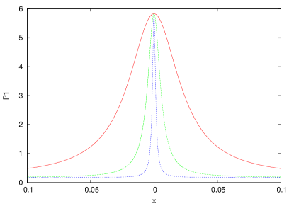
Figure 1: $P_{1}$ vs $x$ at $t=3$ (red), $t=3.5$ (green), and $t=4$ (blue)

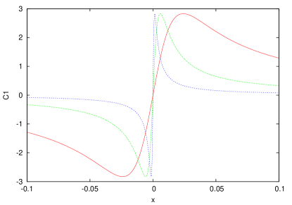
Figure 2: $C_{1}$ vs $x$ at $t=3$ (red), $t=3.5$ (green), and $t=4$ (blue)

Now consider the case where ${C_{10}}=0$. Then $f=0$ for all times and, thus, it follows that ${P_{1}}={P_{+}}$ and ${C_{1}}=0$.

Finally, consider the dependence on spatial position. Suppose that at the initial time there is a region where $C_{1}$ is positive and another region where $C_{1}$ is negative. Define a spatial coordinate $x$ such that $x=0$ is the boundary between the two regions. Then by continuity, we have that ${C_{10}}=0$ at $x=0$. Therefore, we find that for all times ${P_{1}}={P_{+}}$ at $x=0$ while for all other points eventually we have ${P_{1}}={P_{-}}$. The closer to $x=0$ a spatial point is, the smaller the value of $C_{10}$ and, therefore, the longer a time it takes until $f$ at that point becomes large. Thus, though eventually all points near $x=0$ bounce, it takes longer for the nearer points to bounce. Thus, at a given time, a graph of $P_{1}$ vs $x$ will show a peak at $x=0$ and that curve will become more and more steep as time goes on. This is the spike.

As an illustration, consider the case ${C_{10}}=\epsilon x$ with $\epsilon=0.05$ and take ${P_{2}}=2,\,{P_{3}}=1$ and ${t_{0}}=0$. Figure 1 shows $P_{1}$ vs $x$ at $t=3,\,t=3.5$ and $t=4$, while Fig. 2 shows $C_{1}$ vs $x$ at those same times.

III Enhanced Quantization

Besides canonical quantization, which is discussed in Sec. IV, we begin with a very different quantization procedure that avoids the problematic procedure of choosing the right set of canonical variables to promote to canonical operators. The nature of the classical problem features variables that lead to an affine Lie algebra, which is then incorporated in the quantum formulation as affine coherent states. This quantization method is also useful for addressing the issue of the existence of spikes at a semiclassical level.

III.1 Affine algebra

Initially, we propose to quantize the classical system (1)–(2) by making use of the affine coherent states quantization method (see JRK and references therein). We begin with some remarks about use of the affine variables in the classical formulation of the problem. To connect with notation that is more common for affine variables, we make the partial redefinition $(C_{I},P^{J})=:(C_{I},-2D^{J})$, which turns the system (1)–(2) into the traditional Poisson bracket affine formulation,

$$\{D^{I},D^{J}\}=0=\{C_{I},C_{J}\},~{}~{}~{}\{C_{J},D^{I}\}=\delta^{I}_{J}C_{J}\,,$$ (18)

which is called the affine Lie algebra. For the scalar field, we adopt conventional canonical coordinates with the standard Poisson bracket

$$\{\phi,\pi\}=1\,.$$ (19)

For this problem the classical Hamiltonian is constrained to be zero Ashtekar:2011ck , and it is given by

$$H=\frac{1}{2}C^{2}-\sum_{I}C_{I}^{2}+2D^{2}-4\sum_{I}D_{I}^{2}-\frac{1}{2}\pi^{2}=0\,,$$ (20)

where $D=D_{1}+D_{2}+D_{3}$ and $C=C_{1}+C_{2}+C_{3}$. Thus, the dynamics takes the form

$$\dot{D}_{I} = C_{I}(C_{I}-\frac{1}{2}C),$$ (21)

$$\dot{C}_{I} = 2C_{I}(D-2D_{I}),$$ (22)

$$\dot{\pi} = 0,$$ (23)

$$\dot{\phi} = \pi.$$ (24)

Unlike the traditional momentum, which serves to translate the canonical coordinate $C_{I}$, the variable $D^{I}$ serves to dilate $C_{I}$. Thus the affine algebra divides into three sectors: (1) $C_{I}<0$, (2) $C_{I}>0$, and (3) $C_{I}=0$. The first two types are quite similar, while the third type is relatively trivial. Consequently, we will concentrate on types (1) and (2). Thus, it is convenient to define the principal sectors in the kinematical phase space as

$$\Pi_{-}^{I} := \{(C_{I},D^{I})\;|\;C_{I}\in\mathbb{R}_{-},D^{I}\in\mathbb{R}\},$$ (25)

$$\Pi_{+}^{I} := \{(C_{I},D^{I})\;|\;C_{I}\in\mathbb{R}_{+},D^{I}\in\mathbb{R}\}.$$ (26)

III.2 Kinematical Hilbert space

There are two principal, inequivalent, irreducible self-adjoint representations of the Lie algebra (18) corresponding to the sectors (25) and (26). They are defined by the affine quantization principle: $C_{I}\rightarrow\hat{C}_{I}$ and $D^{I}\rightarrow\hat{D}^{I}$, such that

$$[\hat{C}_{I},\hat{C}_{J}]=0=[\hat{D}^{I},\hat{D}^{J}],~{}~{}~{}~{}[\hat{C}_{J},\hat{D}^{I}]=i\hbar\;\delta^{I}_{J}\hat{C}_{J}\;.$$ (27)

The operators $\hat{C}_{I}$ and $\hat{D}^{I}$ are conveniently represented by

$$\hat{D}^{I}f(x^{I}) := -i\hbar/2\;(x^{I}\;\partial/\partial x^{I}+\partial/\partial x^{I}\;x^{I})\;f(x^{I})$$ (28)

$$= -i\hbar\;(x^{I}\;\partial/\partial x^{I}+1/2)\;f(x^{I}),~{}~{}~{}$$

$$\hat{C}_{I}f(x^{I}) := x^{I}f(x^{I})\,,$$ (29)

where $f\in\mathcal{H}^{I}:=span\{L^{2}(\mathbb{R}_{-},dx^{I})\oplus L^{2}(\mathbb{R}_{+},dx^{I})\}$, and where $I=1,2,3$.

For quantization of the scalar field algebra (19) we use the canonical variables and the following representation

$$\hat{\pi}g(\phi):=-i\hbar\;\frac{\partial}{\partial\phi}g(\phi),~{}~{}~{}\hat{\phi}g(\phi):=\phi g(\phi)\,,$$ (30)

where $g\in\mathcal{H}_{\phi}:=L^{2}(\mathbb{R},d\phi)$, so that $[\hat{\phi},\hat{\pi}]=i\hbar\;\mathbb{I}$.

The kinematical Hilbert space $\mathcal{H}$ of the entire system is defined to be

$$\mathcal{H}:=span\{\mathcal{H}^{1}\otimes\mathcal{H}^{2}\otimes\mathcal{H}^{3}\otimes\mathcal{H}_{\phi}\}\,,$$ (31)

which takes into account the usual quantum entanglement of all degrees of freedom.

III.3 Construction of affine coherent states

It is important to observe that the classical Hamiltonian treats the three $C$ variables, as well as the three $D$ variables, in identical fashion in that the Hamiltonian is invariant if the several variables are permuted among themselves. This feature of symmetry is worth preserving in introducing the coherent states for these variables. Thus, the irreducible components of the affine coherent states corresponding to each of the two sectors $\Pi_{-}=\bigcup_{I}\Pi_{-}^{I}$ and $\Pi_{+}=\bigcup_{I}\Pi_{+}^{I}$, are defined as follows

$$|p,q,-\rangle := \prod_{I}|p^{I},q_{I},I,-\rangle$$ (32)

$$:= e^{i\sum_{I}p^{I}\;\hat{C}_{I}/\hbar}e^{-i\sum_{I}\ln(|q_{I}|/\mu)\;\hat{D}_{I}/\hbar}|\eta,-\rangle~{}~{}~{}\mbox{for sector}~{}~{}~{}\Pi_{-}\,,$$

$$|p,q,+\rangle := \prod_{I}|p^{I},q_{I},I,+\rangle$$ (33)

$$:= e^{i\sum_{I}p^{I}\;\hat{C}_{I}/\hbar}e^{-i\sum_{I}\ln(q_{I}/\mu)\;\hat{D}_{I}/\hbar}|\eta,+\rangle~{}~{}~{}\mbox{for sector}~{}~{}~{}\Pi_{+}\,,$$

where $p:=(p^{1},p^{2},p^{3})$ and $q:=(q_{1},q_{2},q_{3})$. The so-called fiducial vectors $|\eta,-\rangle=\otimes_{I}|\eta,I-\rangle$ and $|\eta,+\rangle=\otimes_{I}|\eta,I+\rangle$ are defined by the equations

$$[(\hat{C}_{I}/\mu)+1-i\hat{D}_{I}/(\hbar\beta)]|\eta,I-\rangle = 0\;,$$ (34)

$$[(\hat{C}_{I}/\mu)-1+i\hat{D}_{I}/(\hbar\beta)]|\eta,I+\rangle = 0\;,$$ (35)

where $\mu>0$ and $\beta>0$ denote two free parameters chosen the same for each set of variables $\hat{C}_{I}$ and $\hat{D}_{I}$. (It is also useful to regard $\tilde{\beta}\,[\equiv\hbar\beta]$ and $\hbar$ as two separate parameters for each $I$, especially for approaching the classical limit.) The role of $\mu$ and $\beta$ can be seen in the expressions

$$\langle x|\eta,I+\rangle = Mx^{-1/2}(x/\mu)^{\beta}e^{-\beta(x/\mu)},~{}~{}~{}~{}0<x<\infty\;,$$ (36)

$$\langle x|\eta,I-\rangle = M|x|^{-1/2}(|x|/\mu)^{\beta}e^{-\beta(|x|/\mu)},~{}~{}~{}~{}-\infty<x<0\;,$$ (37)

where $M$ denotes a factor to secure normalization, e.g., $\langle\eta,I\pm|\eta,I\pm\rangle=1$. It follows that

$$\langle\eta,\pm|\hat{C}_{I}|\eta,\pm\rangle=\pm\mu\;,~{}~{}~{}\langle\eta,\pm|\hat{D}_{I}|\eta,\pm\rangle=0\;.$$ (38)

It may happen that the appropriate affine coherent states for our study involve a direct sum of the $+$ and $-$ irreducible versions, such as

$$|p,q,I\rangle:=\theta(q)|p,q,I,+\rangle\oplus\theta(-q)|p,q,I,-\rangle\;,$$ (39)

where $\theta(y):=1$ if $y>0$ and $\theta(y):=0$ if $y<0$. In order to incorporate both the positive and negative spectrum cases for $\{\hat{C_{I}}\}$, we shall use the direct sum of vectors, $|\eta\rangle:=|\eta,+\rangle\oplus|\eta,-\rangle$, in what follows.

In addition to the affine coherent states, we introduce canonical coherent states for the scalar field, which are defined by

$$|\pi,\phi\rangle:=e^{-i\phi\hat{\pi}/\hbar}e^{i\pi\hat{\phi}/\hbar}|\alpha\rangle\;,$$ (40)

where the fiducial vector $|\alpha\rangle$ is chosen (modulo a phase factor) to be the solution to the equation

$$(\omega\hat{\phi}+i\hat{\pi})|\alpha\rangle=0\;,$$ (41)

in which $\omega$ is a free positive parameter. It follows that

$$\langle\pi,\phi|\hat{\pi}|\pi,\phi\rangle=\pi\;,~{}~{}~{}\langle\pi,\phi|\hat{\phi}|\pi,\phi\rangle=\phi\;.$$ (42)

We choose states $|y\rangle$ (previously called $|\phi\rangle$ and which are renamed here to avoid conflicting notation), where $\langle y|y^{\prime}\rangle=\delta(y-y^{\prime})$ and $-\infty<y,y^{\prime}<\infty$, so that $\langle y|\,\hat{\phi}=y\,\langle y|$ as well as $\langle y|\,\hat{\pi}=-i\hbar\partial/\partial y\langle y|$. Thus,

$$(\omega y+\hbar\partial/\partial y)\langle y|\alpha\rangle=0$$ (43)

leads eventually to (with the usual meaning of $\pi$ in the first factor)

$$\langle y|\pi,\phi\rangle=(\omega/\pi\hbar)^{1/4}\,\exp(i\pi y/\hbar-\omega(y-\phi)^{2}/2\hbar)\;.$$ (44)

This last equation asserts that $\langle y|\pi,\phi\rangle$ is the $y$-representation of the coherent state; likewise, it follows that $\langle\pi,\phi|y\rangle\,[\,=\langle y|\pi,\phi\rangle^{*}\,]$ is the coherent-state representation of the $y$-state.

Introducing

$$W_{\pm}:=\prod_{I=1}^{3}|\,\langle\eta,\pm|~{}\hat{C}_{I}^{-1}|\eta,\pm\rangle|\;,$$ (45)

we can get a resolution of unity for each of the two sectors $\Pi_{-}$ and $\Pi_{+}$:

$$\int|\pi,\phi\rangle\langle\pi,\phi|\otimes|p,q,\pm\rangle\langle p,q,\pm|\frac{d\pi\;d\phi\;d^{3}p\;d^{3}q}{h^{4}W_{\pm}}=\mathbb{I}_{\pm}\;$$ (46)

provided that $W_{\pm}<\infty$ (where $h$ denotes Planck’s constant).

III.4 Enhanced classical action functional

The use of coherent states as part of the classical/quantum connection is related to the restricted variation of vectors in the quantum action functional only to appropriate coherent states, which then leads to the enhanced classical action functional, for which $\hbar>0$ throughout. We next spell out this connection.

The quantum action functional is given by

$$A_{Q}=\int_{0}^{T}\langle\psi(t)|[i\hbar(\partial/\partial t)-\hat{H}]|\psi(t)\rangle\,dt$$ (47)

and leads to the Schrödinger equation when general variations are admitted. However, if the variations are limited to coherent states—including just the variations that a macroscopic observer could make—it follows JRK that the so-restricted quantum action functional becomes (with summation on $I$ implied)

$$A_{Q(R)} = \int_{0}^{T}\langle p(t),q(t);\pi(t),\phi(t)|[i\hbar(\partial/\partial t)-\hat{H}]|p(t),q(t);\pi(t),\phi(t)\rangle\,dt$$ (48)

$$= \int_{0}^{T}\{\,-q_{I}(t)\,\dot{p}^{I}(t)+\pi(t)\,\dot{\phi}(t)-H(p(t),\pi(t);q(t),\phi(t))\,\}\;dt\;,$$

where $|p,q;\pi,\phi\rangle:=(|p,q,+\rangle\otimes|\pi,\phi\rangle)\oplus(|p,q,-\rangle\otimes|\pi,\phi\rangle)$, which according to the principles of enhanced quantization JRK can be viewed as the enhanced classical action functional in which $\hbar$ retains its normal positive value. The relation of the quantum Hamiltonian to the expression

$$H(p,\pi;q,\phi):=\langle p,q;\pi,\phi|\,\hat{H}(\hat{C}_{I},\hat{D}_{I};\hat{\pi},\hat{\phi})|p,q;\pi,\phi\rangle$$ (49)

is known as the Weak Correspondence Principle k15 . We can use this relationship to help choose the quantum Hamiltonian $\hat{H}$.

An affine quantization that includes the Weak Correspondence Principle does not involve the assumption that the classical coordinates must be “Cartesian coordinates” as is the case for canonical quantization. This is because in enhanced quantization the variables $p$ and $q$ are not “promoted” to operators in the quantization process. This difference ensures that enhanced quantization can provide different physics than that offered by canonical quantization.

It follows that (no summation intended)

$$H(p,\pi;q,\phi) = \langle p,q;\pi,\phi|\,\hat{H}(\hat{C}_{I},\hat{D}_{I};\hat{\pi},\hat{\phi})\,|p,q;\pi,\phi\rangle$$

$$= \langle\eta;\alpha|\,\hat{H}((q_{I}/\mu)\,\hat{C}_{I},\hat{D}_{I}+p^{I}(q_{I}/\mu)\hat{C}_{I};\hat{\pi}+\pi,\hat{\phi}+\phi)\,|\eta;\alpha\rangle\;,$$

where $|\eta;\alpha\rangle:=|\eta\rangle\otimes|\alpha\rangle$. If we adopt the naive form of the quantum operator $\hat{H}$ suggested by conventional canonical quantization—applied to the classical Hamiltonian (20) —the result leads to [with $\langle(\cdots)\rangle:=\langle\eta;\alpha|(\cdots)|\eta;\alpha\rangle$ in what follows]

$$H(p,\pi;q,\phi) = \frac{1}{2}\langle[\sum_{I}q_{I}(\hat{C_{I}}/\mu)]^{2}\rangle-\sum_{I}q_{I}^{2}\langle(\hat{C}_{I}/\mu)^{2}\rangle$$ (51)

$$~{}~{}~{}\,+2\langle(\sum_{I}[\hat{D}_{I}+p_{I}(q_{I}/\mu)\hat{C}_{I}])^{2}\rangle$$

$$~{}~{}~{}\,-4\sum_{I}\langle(\hat{D}_{I}+p_{I}(q_{I}\hat{C}_{I}/\mu)^{2}\rangle-\frac{1}{2}\langle[\hat{\pi}+\pi^{2}]\rangle\;,$$

which may be written in the form

$$H(p,\pi;q,\phi) = \frac{1}{2}(\sum_{I}q_{I})^{2}-\sum_{I}q_{I}^{2}+2\sum_{I,J}p_{I}q_{I}p_{J}q_{J}-4\sum_{I}p_{I}^{2}q_{I}^{2}-\frac{1}{2}\pi^{2}$$ (52)

$$~{}~{}~{}\,+\frac{1}{2}\sum_{I.J}q_{I}q_{J}[\langle(\hat{C_{I}}/\mu)(\hat{C_{J}}/\mu)\rangle-1]-\sum_{I}q_{I}^{2}[\langle(\hat{C}_{I}/\mu)^{2}\rangle-1]$$

$$~{}~{}~{}\,+2\sum_{I,J}p_{I}q_{I}p_{J}q_{J}\,[\langle[(\hat{C}_{I}/\mu)(\hat{C}_{J}/\mu)]\rangle-1]-4\sum_{I}p_{I}^{2}q_{I}^{2}[\langle(\hat{C}_{L}/\mu)^{2}\rangle-1]$$

$$~{}~{}~{}\,+2\langle(\sum_{I}\hat{D_{I}})^{2}\rangle-4\sum_{I}\langle\hat{D_{I}}^{2}\rangle-\frac{1}{2}\langle\hat{\pi}^{2}\rangle\;.$$

We note that the variables $q_{I}$ and $p_{I}$ are related to the former classical variables according to the relations: $q_{I}:=C_{I}$ and $p_{I}q_{I}:=D_{I}$. Thus, the first line in (52) is the classical Hamiltonian (20), while all the terms in the three remaining lines in (52) are $O(\hbar)$ (based on using the parameters $\tilde{\beta}\,[:=\hbar\beta]$ and $\hbar$). These terms constitute quantum corrections to the classical Hamiltonian generated by the enhanced quantization point of view.

The last line in (52) are constants and can be canceled by subtracting them from $\hat{H}$. The terms on lines two and three involve quantum corrections to line one and are dealt with by adopting the enhanced Hamiltonian given by

$$H(p,\pi;q,\phi) = \frac{1}{2}\langle[\sum_{I}q_{I}(\hat{C_{I}}/\mu)]^{2}\rangle-\sum_{I}q_{I}^{2}\langle(\hat{C}_{I}/\mu)^{2}\rangle$$

$$+2\langle[\sum_{I}p_{I}q_{I}(\hat{C}_{I}/\mu)]^{2}\rangle-4\sum_{I}p_{I}^{2}q_{I}^{2}\langle(\hat{C}_{I}/\mu)^{2}\rangle-\frac{1}{2}\pi^{2}\;,$$

The terms $\langle(\hat{C}_{I}/\mu)\rangle=\pm 1$ while $\langle(\hat{C}_{I}/\mu)^{2}\rangle=1+z$, where

$$z:=-1+$$

$$\;\int_{-\infty}^{\infty}|(x/\mu)|^{2\tilde{\beta}/\hbar+1}\,e^{-(2\tilde{\beta}/\hbar)|(x/\mu)|}\;dx\Big{/}\int_{-\infty}^{\infty}|(x/\mu)|^{2\tilde{\beta}/\hbar-1}\,e^{-(2\tilde{\beta}/\hbar)|(x/\mu)|}\;dx\;,$$

which shows that $z=O(\hbar)$. Equation (III.4) ensures that the enhanced classical Hamiltonian is very much like the traditional classical Hamiltonian, and its enhanced classical equations of motion involve small corrections to the traditional classical equations of motion.

IV Passing to the physical Hilbert space

The constraint of the Hamiltonian vanishing is an essential requirement in the quantum theory as it was in the classical theory. This has the effect of reducing the kinematical Hilbert space to the physical Hilbert space. In other words, we propose to follow the Dirac quantization scheme PAM ; HT : first, quantize (in the kinematical Hilbert space) then second, introduce the constraints (to identify the physical Hilbert space). We realize this scheme with the help of reproducing kernel Hilbert spaces (see, e.g., Klauder:2006rs ; NA ).

IV.1 Reproducing kernel Hilbert space

The essence of reproducing kernel Hilbert spaces is readily explained. For example, as we have seen, the kinematical Hilbert space is spanned by the set of coherent states $|p,q;\pi,\phi\rangle$. Thus, every vector in that space is given by

$$|\Psi\rangle=\sum_{k}a_{k}\;|p_{k},q_{k};\pi_{k},\phi_{k}\rangle\;,$$ (55)

provided that

$$0\leq\langle\Psi|\Psi\rangle=\sum_{j,k}a^{*}_{j}a_{k}\langle p_{j},q_{j};\pi_{j},\phi_{j}|p_{k},q_{k};\pi_{k},\phi_{k}\rangle<\infty\;.$$ (56)

Observe that the set of coherent states, $\{|p,q;\pi,\phi\rangle\}$, forms a continuously labeled set of vectors, which spans the kinematical Hilbert space, but whose elements are, therefore, not linearly independent as in a conventional basis set. Instead, the set of coherent states represents a kind of “continuous basis” for a separable Hilbert space.

Next, we give a functional representation for every abstract vector by introducing

$$\Psi(p,q;\pi,\phi):=\langle p,q;\pi,\phi|\Psi\rangle=\sum_{k}a_{k}\;\langle p,q;\pi,\phi|p_{k},q_{k};\pi_{k},\phi_{k}\rangle\;.$$ (57)

Another vector is given by its functional representation as follows

$$\Phi(p,q;\pi,\phi)=\langle p,q;\pi,\phi|\Phi\rangle=\sum_{j^{\prime}}b_{j^{\prime}}\;\langle p,q;\pi,\phi|p_{j^{\prime}},q_{j^{\prime}};\pi_{j^{\prime}},\phi_{j^{\prime}}\rangle\;,$$ (58)

where the set $\{p_{j^{\prime}},q_{j^{\prime}};\pi_{j^{\prime}},\phi_{j^{\prime}}\}$ for $|\Phi\rangle$ is generally different from the set $\{p_{k},q_{k};\pi_{k},\phi_{k}\}$ for $|\Psi\rangle$. In the reproducing kernel Hilbert space, the inner product of two such functional representation elements is given by

$$(\Phi,\,\Psi):=\sum_{j^{\prime},k}b^{*}_{j^{\prime}}a_{k}\langle p_{j^{\prime}},q_{j^{\prime}};\pi_{j^{\prime}},\phi_{j^{\prime}}|p_{k},q_{k};\pi_{k},\phi_{k}\rangle\;,$$ (59)

which is just a functional representative of $(\Phi,\Psi)=\langle\Phi|\Psi\rangle$.

Observe that the inner product of two coherent states, $\langle p_{j^{\prime}},q_{j^{\prime}};\pi_{j^{\prime}},\phi_{j^{\prime}}|p_{k},q_{k};\pi_{k},\phi_{k}\rangle$, serves as a reproducing kernel; if the vector $\langle\Phi|$ is chosen as the vector $\langle p,q;\pi,\phi|$ (i.e., $b_{j^{\prime}}=\delta_{j^{\prime},1})$, then the result of the inner product “reproduces” the expression for $\langle p,q;\pi,\phi|\Psi\rangle$. Traditionally, the reproducing kernel is chosen as jointly continuous in both arguments. In our case, the reproducing kernel using coherent states is automatically jointly continuous because the group properties of the affine and canonical groups ensure continuity. Hence, like all reproducing kernel Hilbert spaces, our reproducing kernel Hilbert space is composed entirely of continuous functions.

IV.2 Coherent state overlap as a reproducing kernel

The foregoing discussion is based on the general theory of reproducing kernel Hilbert spaces. However, when suitable coherent states generate the reproducing kernel, as in the present case, some additional properties hold true. In particular, there is an equivalent, second procedure for the inner product of two functional representatives. Equation (46) shows that a suitable integral over projection operators onto coherent states leads to the unit operator in the kinematical Hilbert space. Choosing the positive section as an example, the general coherent state matrix elements of that equation lead to the equation

$$\langle p^{\prime\prime},q^{\prime\prime};\pi^{\prime\prime},\phi^{\prime\prime}|p^{\prime},q^{\prime};\pi^{\prime},\phi^{\prime}\rangle=\int\langle p^{\prime\prime},q^{\prime\prime};\pi^{\prime\prime},\phi^{\prime\prime}|p,q;\pi,\phi\rangle\langle p,q;\pi,\phi|p^{\prime},q^{\prime};\pi^{\prime},\phi^{\prime}\rangle\;d\mu(p,q;\pi,\phi)\;,$$ (60)

where $d\mu$ represents the integration measure in (46). It follows from this equation that the inner product of the two functional representatives $\Phi(p,q;\pi,\phi)=\langle p,q;\pi,\phi|\Phi\rangle$ and $\Psi(p,q;\pi,\phi)=\langle p,q;\pi,\phi|\Psi\rangle$ is given by

$$\langle\Phi|\Psi\rangle=\int\Phi^{*}(p,q;\pi,\phi)\,\Psi(p,q;\pi,\phi)\;d\mu(p,q;\pi,\phi)\;.$$ (61)

In particular, if $\langle\Phi|=\langle p^{\prime\prime},q^{\prime\prime};\pi^{\prime\prime},\phi^{\prime\prime}|$, this relation leads to an example of the reproducing kernel property. Indeed, if one lets $f(p,q,\pi,\phi)$ be a general element of the space $L^{2}(\mathbb{R}^{8})$, the reproducing kernel acts as a projection operator onto a valid vector in the kinematical Hilbert space, e,g.,

$$\Psi_{f}(p^{\prime},q^{\prime};\pi^{\prime},\phi^{\prime})=\int\langle p^{\prime},q^{\prime};\pi^{\prime},\phi^{\prime}|p,q;\pi,\phi\rangle\,f(p,q,\pi,\phi)\;d\mu(p,q;\pi,\phi)\;.$$ (62)

It may well be that dealing with this integral version of the inner product is more appropriate in special cases.

IV.3 Projection operators for reducing the kinematical Hilbert space

Let ${\rm I}\hskip-1.99997pt{\rm E}$ represent a projection operator (hence, ${\rm I}\hskip-1.99997pt{\rm E}^{2}={\rm I}\hskip-1.99997pt{\rm E}^{\dagger}={\rm I}\hskip-1.99997pt{\rm E}$). If ${\rm I}\hskip-1.99997pt{\rm E}$ is smaller then the unit operator, it follows that $\langle p,q;\pi,\phi|\,{\rm I}\hskip-1.99997pt{\rm E}\,|p^{\prime},q^{\prime};\pi^{\prime},\phi^{\prime}\rangle$ serves as a reproducing kernel for a subspace of the original Hilbert space. In particular, we suppose that ${\rm I}\hskip-1.99997pt{\rm E}$ is a projection operator onto the subspace where the Hamiltonian vanishes, i.e., ${\rm I}\hskip-1.99997pt{\rm E}={\rm I}\hskip-1.99997pt{\rm E}(\hat{H}=0)$. The Hamiltonian operator consists of two parts one with $\hat{C}_{I}$ and $\hat{D}_{I}$ and the other with $\hat{\pi}^{2}/2$. Let us assume that the first part of $\hat{H}$ has a discrete spectrum $\{E_{n}\geq 0\}$ and that the second part has a continuous spectrum $0\leq y^{2}/2<\infty$. Thus, the eigenfunctions $|E_{n};y\rangle=|E_{n}\rangle\otimes|y\rangle$, satisfy $\hat{H}\,|E_{n};y\rangle=(E_{n}-y^{2}/2)\,|E_{n};y\rangle$ and $\langle E_{n};x|E_{m};y\rangle=\delta_{nm}\delta(x-y)$. Suppose the full spectrum of $\hat{H}$ implies that $\Sigma_{n}\int_{0}^{\infty}|E_{n};y\rangle\langle E_{n};y|\;dy$ is the unit operator. In such a case we have

$$\langle p,q;\pi,\phi|{\rm I}\hskip-1.99997pt{\rm E}|p^{\prime},q^{\prime};\pi^{\prime},\phi^{\prime}\rangle=\sum_{n}\langle p,q|E_{n}\rangle\langle E_{n}|p^{\prime},q^{\prime}\rangle\,\langle\pi,\phi|\sqrt{2E_{n}}\rangle\langle\sqrt{2E_{n}}|\pi^{\prime},\phi^{\prime}\rangle\;.$$ (63)

It follows that Eq. (63) defines a valid representation of a reproducing kernel that includes only the subspace where $\hat{H}=0$. Therefore, a functional representation for every vector $\Psi_{{\rm I}\hskip-1.39998pt{\rm E}}$ of our physical Hilbert is given by

$$\Psi_{{\rm I}\hskip-1.39998pt{\rm E}}(p,q;\pi,\phi)=\langle p,q;\pi,\phi|\Psi_{{\rm I}\hskip-1.39998pt{\rm E}}\rangle=\sum_{k}a_{k}\;\langle p,q;\pi,\phi|{\rm I}\hskip-1.99997pt{\rm E}|p_{k},q_{k};\pi_{k},\phi_{k}\rangle\;.$$ (64)

Operators for the kinematical Hilbert space lead to generally different operators for the physical Hilbert space. Since the affine coherent state vectors $\{|p,q;\pi,\phi\rangle\}$ span the kinematical Hilbert space, it follows that the projected coherent state vectors $\{{\rm I}\hskip-1.99997pt{\rm E}|p,q;\pi,\phi\rangle\}$ span the physical Hilbert space, as described above. In like fashion, an operator $\hat{A}$ that applies to the kinematical Hilbert space leads to an operator $\hat{A}_{{\rm I}\hskip-1.39998pt{\rm E}}:={\rm I}\hskip-1.99997pt{\rm E}\hat{A}{\rm I}\hskip-1.99997pt{\rm E}$ that applies to the physical Hilbert space. Sometimes a general property of $\hat{A}$ is not preserved by $\hat{A}_{{\rm I}\hskip-1.39998pt{\rm E}}$, such as being self adjoint. If $\hat{A}\geq 0$, then $\hat{A}_{{\rm I}\hskip-1.39998pt{\rm E}}\geq 0$ as well, and if $\hat{A}$ is self adjoint then $\hat{A}_{{\rm I}\hskip-1.39998pt{\rm E}}$ can also be chosen to be self adjoint. On the other hand, if $\hat{Q}$ and $\hat{P}$ (with $[\hat{Q},\hat{P}]=i\hbar\,\mathbb{I}$) are both self adjoint and a projection operator ${\rm I}\hskip-1.99997pt{\rm F}$ is such that ${\rm I}\hskip-1.99997pt{\rm F}\hat{Q}{\rm I}\hskip-1.99997pt{\rm F}$ is self adjoint and strictly positive, then it follows that ${\rm I}\hskip-1.99997pt{\rm F}\hat{P}{\rm I}\hskip-1.99997pt{\rm F}$ can never be self adjoint. This is just the situation that is overcome by choosing the affine variables $\hat{Q}$ and $\hat{D}:=(1/2)[\hat{Q}\hat{P}+\hat{P}\hat{Q}]$ (with $[\hat{Q},\hat{D}]=i\hbar\hat{Q}$) for which $\hat{Q}>0$ and $\hat{D}$ are both self adjoint.

Note that elements of the physical Hilbert space enjoy the same integral representation of inner products as noted earlier since

$$\langle\Phi|{\rm I}\hskip-1.99997pt{\rm E}|\Psi\rangle=\int\Phi_{{\rm I}\hskip-1.39998pt{\rm E}}^{*}(p,q;\pi,\phi)\,\Psi_{{\rm I}\hskip-1.39998pt{\rm E}}(p,q;\pi,\phi)\;d\mu(p,q;\pi,\phi)\;,$$ (65)

where, as before, $\Psi_{{\rm I}\hskip-1.39998pt{\rm E}}(p,q;\pi,\phi):=\langle p,q;\pi,\phi|{\rm I}\hskip-1.99997pt{\rm E}|\Psi\rangle$.

The development with time $(t)$ in the kinematical Hilbert space follows traditional expressions, such as if $\hat{H}(t)$ denotes the (possibly time dependent) Hamiltonian operator that acts on an operator $\hat{A}(t)$ for which the time dependence is only that caused by the Hamiltonian, i.e., for which $\partial A(t)/\partial t=0$, then the Heisenberg equation of motion $i\hbar\,d\hat{A}(t)/dt=[\hat{A}(t),\hat{H}(t)]$ holds as usual. On the other hand, for the physical Hilbert space, one must impose the projection operator after forming the commutator such as $i\hbar\,{\rm I}\hskip-1.99997pt{\rm E}d\hat{A}(t)/dt{\rm I}\hskip-1.99997pt{\rm E}={\rm I}\hskip-1.99997pt{\rm E}[\hat{A}(t),\hat{H}(t)]{\rm I}\hskip-1.99997pt{\rm E}$ and not by imposing the projection operator before forming the commutator in the form $i\hbar\,d{\rm I}\hskip-1.99997pt{\rm E}\hat{A}(t){\rm I}\hskip-1.99997pt{\rm E}/dt=[{\rm I}\hskip-1.99997pt{\rm E}\hat{A}(t){\rm I}\hskip-1.99997pt{\rm E},{\rm I}\hskip-1.99997pt{\rm E}\hat{H}(t){\rm I}\hskip-1.99997pt{\rm E}]$. Not only does the latter equation involve a different number of projection operators $({\rm I}\hskip-1.99997pt{\rm E})$ on each side of the equation, but, as we expect in the current problem, the physical Hilbert space is such that ${\rm I}\hskip-1.99997pt{\rm E}\hat{H}(t){\rm I}\hskip-1.99997pt{\rm E}=0$. Consequently, for the former equation of motion, the operators ${\rm I}\hskip-1.99997pt{\rm E}\hat{A}(t){\rm I}\hskip-1.99997pt{\rm E}$ evolve properly within the physical Hilbert space for suitable choices of the operator $\hat{A}(t)$.

It is noteworthy that the energy eigenstates for the first part of the Hamiltonian (i.e., only with $\hat{C}$ and $\hat{D}$) are degenerate leading to the possibility that there may be various energy eigenstates for a single energy value. This is likely to be true as well for the energy value $E=0$. Thus, there could be a family of zero-energy eigenstates for which $\hat{\pi}^{2}/2$ is not required to ensure that $\hat{H}\,|m:(E=0)\rangle=0$, $m\in\{1,2,3,...\}$. In such a case only affine coherent states, $|p,q\rangle$, are necessary and no canonical coherent states, $|\pi,\phi\rangle$, are needed. To find the states $|m:(E=0)\rangle$ requires solving the zero-energy Schrödinger equation $\hat{H}|m:(E=0)\rangle=0$. It is important to understand that the form of the differential equation leading to zero-energy solutions in the canonical quantization scheme in the following section is entirely different from the differential equation leading to zero-energy solutions in the affine quantization scheme as the latter equation is shown in the following section. Besides that difference in formulation, there is one advantage that an affine quantization offers in that the proper subtraction terms can be decided so that the enhanced classical Hamiltonian has the form given in (III.4) such that, even when $\hbar>0$, the enhanced classical solutions follow when the enhanced classical Hamiltonian is constrained to vanish.

V Affine Quantization

Let us try to define $\hat{H}$ by making use of the classical form of $H$ defined by Eq. ​(20). Since there are no products of $C_{I}$ and $D_{I}$ in (20), and due to (27), the mapping of the Hamiltonian (20) into a Hamiltonian operator is straightforward. We get

$$\hat{H} = \frac{1}{2}(\sum_{I}x_{I})^{2}-\sum_{I}x_{I}^{2}-2\hbar^{2}[\sum_{I}\,(x_{I}\frac{\partial}{\partial x_{I}}+1/2)\,]^{2}$$ (66)

$$\hskip 30.00005pt+4\hbar^{2}\sum_{I}\,(x_{I}\frac{\partial}{\partial x_{I}}+1/2)^{2}+\frac{1}{2}\hbar^{2}\frac{\partial^{2}}{\partial\phi^{2}}$$

$$= \hbar^{2}\big{(}-\frac{3}{2}+2\sum_{I}x_{I}^{2}\frac{\partial^{2}}{\partial x_{I}^{2}}-4\sum_{I<J}x_{I}x_{J}\frac{\partial^{2}}{\partial x_{I}\partial x_{J}}\big{)}$$

$$\hskip 30.00005pt+\sum_{I<J}x_{I}x_{J}-\frac{1}{2}\sum_{I}x_{I}^{2}+\frac{\hbar^{2}}{2}\frac{\partial^{2}}{\partial\phi^{2}}=:\hat{H}_{g}+\hat{H}_{\phi}\;,$$

where $\hat{H}_{\phi}=\frac{\hbar^{2}}{2}\frac{\partial^{2}}{\partial\phi^{2}},$ and where $\hat{H}_{g}$ is the gravitational contribution.

One can show (see Appendix ) that the operator $\hat{H}$ is Hermitian on a dense subspace of $L^{2}(\mathbb{R}^{3},d^{3}x)$ of the functions satisfying suitable boundary conditions.

VI Canonical quantization

Though we think that the form of the Poisson brackets given in Eqs. ​(1) indicates that our system is best treated with affine quantization methods, we nonetheless briefly consider how this system might be treated using the more usual canonical quantization methods. Recall that in canonical quantization one begins with classical configuration variables $X_{I}$ and momentum variables $P_{I}$ having Poisson brackets,

$$\{P^{I},X_{J}\}={\delta^{I}_{\,J}}$$ (67)

One then realizes the kinematical Hilbert space as $L^{2}(\mathbb{R},dX_{I})$ and the operator $P^{I}$ as ${P^{I}}=i\hbar\,(\partial/\partial{X_{I}})$.

Now consider the case where all $C_{I}$ are positive and define the $X_{I}$ by ${X_{I}}=(1/2)\ln{C_{I}}$. Then it follows from Eq. ​(1) that $P^{I}$ and $X_{I}$ satisfy the canonical Poisson bracket given in Eq. ​(67).

The Hamiltonian constraint [Eq. ​(2)] written in terms of $X_{I}$ then becomes

$${{\left({e^{2{X_{1}}}}+{e^{2{X_{2}}}}+{e^{2{X_{3}}}}\right)}^{2}}-2\left({e^{4{X_{1}}}}+{e^{4{X_{2}}}}+{e^{4{X_{3}}}}\right)$$

$$+{{\left({P_{1}}+{P_{2}}+{P_{3}}\right)}^{2}}-2\left({P_{1}^{2}}+{P_{2}^{2}}+{P_{3}^{2}}\right)-{\pi^{2}}=0\,.$$ (68)

The physical Hilbert space is obtained by replacing $P_{I}$ by $i\hbar\,(\partial/\partial{X_{I}})$ and then imposing the Hamiltonian constraint as an operator acting on the wave function $\psi$. We, thus, obtain the following equation:

$${\hbar^{2}}{\frac{{\partial^{2}}\psi}{\partial{\phi^{2}}}}={\hbar^{2}}\left(\sum_{I\neq J}\frac{\partial^{2}\psi}{\partial{X_{I}}\partial{X_{J}}}-\sum_{I}\frac{\partial^{2}\psi}{\partial X_{I}^{2}}\right)+\left(\sum_{I}{e^{4{X_{I}}}}-\sum_{I\neq J}e^{2({X_{I}}+{X_{J}})}\right)\psi\;.$$ (69)

The rhs of Eq. ​(69) defines an Hermitian operator on a dense subspace of $L^{2}(\mathbb{R}^{3},d^{3}X)$ of the functions satisfying suitable boundary conditions.

VII Methods of imposing the Hamiltonian constraint

In order to find the quantum fate of spikes, we will need to impose the Hamiltonian constraint, possibly using numerical methods, and examine the properties of the resulting wave function $\psi$. Note that in ordinary quantum mechanics the Hamiltonian operator generally involves the Laplacian, and the energy eigenvalue equation (“time-independent Schrödinger equation”) is an elliptic equation. However, it is a general property of quantum cosmology that the quantum Hamiltonian constraint equation is a hyperbolic equation. (This strange property is essentially due to the conformal degree of freedom of the metric behaving differently from the other metric degrees of freedom.) In contrast to elliptic equations, which lead to boundary value problems, hyperbolic equations lead to initial value problems. To pose the initial value problem, one must choose a timelike coordinate $T$ and choose initial data on a surface of constant $T$.

For the case of canonical quantization and the imposition of (69), a convenient choice of coordinates is the following:

$$T:={X_{1}}+{X_{2}}+{X_{3}}\,,$$ (70)

$$Y:={X_{1}}-{X_{2}}\,,$$ (71)

$$Z:={\textstyle{\frac{1}{2}}}({X_{1}}+{X_{2}})-{X_{3}}\,,$$ (72)

which turns (69) into

$${\hbar^{2}} \left(-{\frac{{\partial^{2}}\psi}{\partial{T^{2}}}}+{\textstyle{\frac{4}{3}}}{\frac{{\partial^{2}}\psi}{\partial{Y^{2}}}}+{\frac{{\partial^{2}}\psi}{\partial{Z^{2}}}}+{\textstyle{\frac{1}{3}}}{\frac{{\partial^{2}}\psi}{\partial{\phi^{2}}}}\right)$$ (73)

$$+ \frac{1}{3}\,{e^{(4/3)(T+Z)}}\left[2\left(1+{e^{Y-2Z}}+{e^{-(Y+2Z)}}\right)-\left({e^{2Y}}+{e^{-2Y}}+{e^{-4Z}}\right)\right]\psi=0\;,$$

where $\psi\in L^{2}(R^{4},dTdYdZd\phi)$. Equation (73) has explicitly a hyperbolic form, suitable for numerical simulations, with $T$ playing the role of an evolution parameter.

For the case of affine quantization, the Hamiltonian defined by Eq. ​(66) yields an equation analogous to Eq. ​(69), which is defined in $L^{2}(R^{4},d^{3}xd\phi)$ and reads

$${\hbar^{2}}{\frac{{\partial^{2}}\psi}{\partial{\phi^{2}}}}=4{\hbar^{2}}\left(\sum_{I\neq J}x_{I}x_{J}\frac{\partial^{2}\psi}{\partial{x_{I}}\partial{x_{J}}}-\sum_{I}x^{2}_{I}\frac{\partial^{2}\psi}{\partial x_{I}^{2}}+\frac{3}{4}\psi\right)+\left(\sum_{I}x^{2}_{I}-\sum_{I\neq J}x_{I}x_{J}\right)\psi\;.$$ (74)

The solution $\psi$ of Eq. ​(74) has, potentially, a very different physical interpretation than that of the solution of Eq. ​(69).

One can diagonalize Eq. (74) in a similar way as Eq. ​(69). Introducing the variables,

$$T:= x_{1}x_{2}x_{3},$$ (75)

$$Y:= \frac{x_{1}}{x_{2}},$$ (76)

$$Z:= \frac{\sqrt{x_{1}x_{2}}}{x_{3}},$$ (77)

enables rewriting (74) in the following form:

$$4{\hbar^{2}}\left(-{T^{2}\frac{{\partial^{2}}\psi}{\partial{T^{2}}}}+{\textstyle{\frac{4}{3}}}{Y^{2}\frac{{\partial^{2}}\psi}{\partial{Y^{2}}}}+{Z^{2}\frac{{\partial^{2}}\psi}{\partial{Z^{2}}}}+\frac{1}{12}{\frac{{\partial^{2}}\psi}{\partial{\phi^{2}}}}-4T\frac{\partial\psi}{\partial T}+{\textstyle{\frac{4}{3}}}Y\frac{\partial\psi}{\partial Y}+Z\frac{\partial\psi}{\partial Z}-\frac{3}{4}\psi\right)$$

$$+{\frac{1}{3}}\,{(TZ)^{2/3}}\left[\left({Y^{2}}+{Y^{-2}}+{Z^{-4}}\right)-2\left(1+\frac{Y}{Z^{2}}+\frac{1}{YZ^{2}}\right)\right]\psi=0\;.$$ (78)

In this hyperboliclike equation, suitable for numerical simulations, the variable $T$ plays the role of an evolution parameter.

VIII Exploring the Affine Constraint Equation

We recall the affine Hamiltonian constraint equation (74) and set the left-hand side to zero seeking a solution with only $\{x_{I}\}$ variables. It follows that a “near solution” to the resulting constraint equation is given by

$$\Psi(x_{1},x_{2},x_{3}):=(2\hbar)^{-3/2}\,\exp\{-(1/2\hbar)[\sum_{I}\,|x_{I}|\hskip 0.80002pt]\hskip 0.80002pt\}\;,$$ (79)

and, as presented, $\Psi$ is normalized, i.e., $\int|\Psi(x_{1},x_{2},x_{3})|^{2}\,d^{3}\!x=1$. If we now put the remaining zero-point energy [appearing as $3\hbar^{2}$ in (74)] as part of the original Hamiltonian, this solution satisfies the equation $\hat{H}\,\Psi=0$, and, thus, (79) represents a solution of the quantum constraint. At first sight it seems strange that a function that has a discontinuous derivative—thanks to $|x_{1}|$, etc.—can satisfy the modified (74). In fact, all eight independent solutions of the modified affine Hamiltonian constraint (74) have a similar form given by

$$\Psi(x_{1},x_{2},x_{3};J_{\pm}):=(\hbar)^{-3/2}\,\Pi_{I}\,\{\,[J_{+,I}\theta(x_{I})+J_{-,I}\theta(-x_{I})]\,e^{-(1/2\hbar)\,|x_{I}|}\,\}\;,$$ (80)

where $\theta(y):=1$ for $y>0$ and $\theta(y):=0$ for $y<0$, and $|J_{+,I}|^{2}+|J_{-,I}|^{2}=1$ for each $I$. This form of the wave function contains finite jumps at $x_{I}=0$ when $|J_{+,I}|\not=|J_{-,I}|$, for one or more $I$. The solution (80) is valid even though there are terms of the form $x_{I}^{2}\,\delta\,^{\prime}(x_{I})$ as well as $x_{I}x_{J}\,\delta(x_{I})\,\delta(x_{j})$ for $I\not=J$, all of which vanish. The factor $8\,[=2^{3}]$ arises from the variety available from the eight inequivalent terms $J_{\pm,1}\,J_{\pm,2}\,J_{\pm,3}$. Hereafter, to simplify the notation in this section, we assume that the plain symbol $\Psi$ (or $\Phi$) denotes any vector in the eight-dimensional physical Hilbert space with the form given in (80).

It is noteworthy that certain operators can be simplified when they are confined to act on vectors in the physical Hilbert space. Clearly, the relation $\hat{C}_{I}\,\Psi=x_{I}\,\Psi$ holds, and it follows that

$$\hat{D}_{I}\,\Psi=-i\hbar[x_{I}\,\partial/\partial x_{I}+1/2]\,\Psi=(i/2)[\,x_{I}-\hbar]\,\Psi=(i/2)[\,\hat{C}_{I}-\hbar]\,\Psi\;,$$ (81)

which shows that the action of $\hat{D}_{I}$ is effectively multiplicative in nature. Indeed, it follows that

$$\hat{D}_{I}\,\hat{C}^{p}_{I}\,\Psi=\{\,[\hat{D}_{I},\,\hat{C}^{p}_{I}]+\hat{C}^{p}_{I}\,\hat{D}_{I}\}\,\Psi=\{-i\hbar\,p\,\hat{C}^{p}_{I}+(i/2)\hat{C}^{p}_{I}\,[\hat{C}_{I}-\hbar]\}\,\Psi\;.$$ (82)

Although these equations are correct, however, it follows that while $\Psi$ is a vector in the physical Hilbert space, it is a fact that $\hat{C}^{p}_{I}\,\Psi$, for $p>0$, is not a vector in the physical Hilbert space. To address that situation, we can obtain the part of that vector in the physical Hilbert space by taking the inner product with another vector $\Phi$ in the physical Hilbert space, which leads to $(\Phi,\hat{C}^{p}_{I}\,\Psi)$. In the eight-dimensional physical Hilbert space, this inner product, for $I=1$, becomes

$$(\Phi,\hat{C}^{p}_{1}\,\Psi)=\hbar^{-1}\,\int\,[K_{+,1}^{*}\theta(x_{1})+K_{-,1}^{*}\theta(-x_{1})]$$

$$\hskip 80.00012pt\times\,[J_{+,1}\theta(x_{1})+J_{-,1}\theta(-x_{1})]\,\,x^{p}_{1}\,e^{-|x_{1}|/\hbar}\,dx_{1}$$

$$\hskip 45.00006pt=p!\,\hbar^{p}\,[K_{+,1}^{*}J_{+,1}+(-1)^{p}K_{-,1}^{*}J_{-,1}]\;,$$ (83)

where $J_{\pm,1}$ refers to $\Psi$ and $K_{\pm,1}$ refers to $\Phi$.

This simplification of the form taken by the operator $\hat{D}_{I}$ leads to a simplification of the equation of motion. The classical equations $\dot{C}_{I}=C_{I}[D_{I}-2D]$ transform, for the kinematical Hilbert space, to the operator equation

$$\dot{\hat{C}}_{I}=(1/2)\hat{C}{{}_{I}}\,[\hat{D}_{I}-2\hat{D}]+(1/2)[\hat{D}_{I}-2\hat{D}]\,\hat{C}{{}_{I}}\;.$$ (84)

To fit it into the physical Hilbert space, this equation becomes

$$(\Phi,\,\dot{\hat{C}}_{I}\,\Psi)=(1/2)\,(\Phi,\,\{\,\hat{C}{{}_{I}}\,[\hat{D}_{I}-2\hat{D}]+[\hat{D}_{I}-2\hat{D}]\,\hat{C}{{}_{I}}\}\,\Psi)\;,$$ (85)

which becomes an equation involving only the $\{\hat{C}_{I}\}$ operators, namely

$$(\Phi,\,\dot{\hat{C}}_{I}\,\Psi)=(1/2)\,(\Phi,\,\{\,-i\hbar\,\hat{C}_{I}+i\hat{C}_{I}(\hat{C}_{I}-\hbar)+2\sum_{L}\,[\,i\hbar\,\hat{C}_{L}-i\hat{C}_{L}\,(\hat{C}_{L}-\hbar)]\,\}\,\Psi)\,.$$ (86)

It follows that higher-order time derivatives of $\hat{C}$ can be developed leading to an expression of the form

$$\hat{C}_{I}(t)=\hat{C}_{I}(0)+t\,\dot{\hat{C}}_{I}(0)+(t^{2}/2)\,\ddot{\hat{C}}_{I}(0)+...\;,$$ (87)

which leads to the general expression given by

$$(\Phi,\,\hat{C}_{I}(t)\,\Psi)=(\Phi,\,M_{I}(t,\hat{C}_{L}(0))\,\Psi)$$ (88)

which introduces the time dependent, $8\times 8$ matrix, $M_{I}(t,\hat{C}_{L}(0))$.

Observe that the matrix $M_{I}$ itself does not depend on any specific vector in the physical Hilbert space. The vectors in the physical Hilbert space are distinguished by the factors $J_{\pm,I}$ that signify the coefficients that define a given vector $\Psi$. To discuss position dependence in real space, as was the case in Sec. II in order to study the position dependence of potential spikes, we let $\bar{x}_{1}$ represent a position in real space. For us, dealing with the physical Hilbert space, the position parameter appears in the choice of the parameters $J_{\pm,I}$ in the physical Hilbert space vectors; the position parameter $\bar{x}_{1}$ does not appear in the matrix $M_{I}(t,\hat{C}_{L}(0))$. Let us first choose the initial position of a vector to be at position $\bar{x}_{1}=0$ in space. This we can accommodate by choosing $J_{+,1}=J_{-,1}=1/\sqrt{2}$. If, instead, we want to be at a small, nonzero position $0<\bar{x}_{1}<\hbar$, we can choose $J_{+,1}=\sqrt{(1+\bar{x}_{1}/\hbar)/2}$ and $J_{-,1}=\sqrt{(1-\bar{x}_{1}/\hbar)/2}$ so that

$$(\hbar)^{-1}\int[|J_{+,1}|^{2}\theta(x_{1})+|J_{-,1}|^{2}\theta(-x_{1})]\,x_{1}\,\exp[-|x_{1}|/\hbar\,]\,dx_{1}=\bar{x}_{1}\;.$$ (89)

Using the several tools discussed above, let us consider some general properties of the expression for $(\Psi(\bar{x}_{1}),\,\hat{C}(t)\,\Psi(\bar{x}_{1})\,)$, focusing on the influence of the space position $\bar{x}_{1}$. With $\Psi(0):=\Psi(\bar{x}_{1}=0)$, we observe that

$$\hskip-20.00003pt|\;(\Psi(\bar{x}_{1}),\,\hat{C}_{1}(t)\,\Psi(\bar{x}_{1})\,)-(\Psi(0),\,\hat{C}_{1}(t)\,\Psi(0)\,)\,|$$

$$=|\;(\Psi(\bar{x}_{1}),\,\hat{C}_{1}(t)\,\Psi(\bar{x}_{1})\,)-(\Psi(0),\,\hat{C}_{1}(t)\,\Psi(0)\,)$$

$$\hskip 30.00005pt+(\Psi(0),\,\hat{C}_{1}(t)\,\Psi(\bar{x}_{1})\,)-(\Psi(0),\,\hat{C}_{1}(t)\,\Psi(\bar{x}_{1})\,)\,|$$

$$\leq|(\Psi(\bar{x}_{1}),\,\hat{C}_{1}(t)\,\Psi(\bar{x}_{1})\,)-(\Psi(0),\,\hat{C}_{1}(t)\,\Psi(\bar{x}_{1})\,)\,|$$

$$\hskip 30.00005pt+|(\Psi(0),\,\hat{C}_{1}(t)\,\Psi(\bar{x}_{1})\,)-(\Psi(0),\,\hat{C}_{1}(t)\,\Psi(0)\,)\,|$$ (90)

$$\leq||\Psi(\bar{x}_{1})-\Psi(0)||\,||\hat{C}_{1}(t)\,\Psi(\bar{x}_{1}||+||\Psi(\bar{x}_{1})-\Psi(0)||\,||\hat{C}_{1}(t)^{\dagger}\,\Psi(0)||\;,$$

where $||\Psi||$ denotes the norm of the vector $\Psi$. Finally, with the vectors $\Psi$ normalized to unity, we find that

$$|\;(\Psi(\bar{x}_{1}),\,\hat{C}_{1}(t)\,\Psi(\bar{x}_{1})\,)-(\Psi(0),\,\hat{C}_{1}(t)\,\Psi(0)\,)\,|\leq 2\,||\Psi(\bar{x}_{1})-\Psi(0)||\,\,||\hat{C}_{1}(t)||\,,$$

in which $||\hat{C}_{1}(t)||$ now denotes the operator norm of the $8\times 8$ matrix representation of the physical Hilbert space form, i.e., $M_{1}(t,\hat{C}_{L}(0))$, of the given operator. Moreover, this equation provides a bound on the hypothetical quantum spike, and with the temporal and spacial portions bounded and completely separated, we believe that quantum spikes do not exist. In other words, these solutions do not support the existence of quantum spikes since they prohibit the temporal and spatial behavior characteristic of the classical spike behavior.

To achieve the eight solutions of the quantum Hamiltonian constraint we had to subtract a numerical term that was proportional to $\hbar^{2}$. This is not unlike using normal ordering to find solutions of a quantum problem, e.g., removing the zero-point energy in a free field when it is composed of a set of harmonic oscillators. Although our problem has been treated as a quantum mechanics problem, it should be appreciated that such a problem applies to every spatial point and, thus, the overall zero-point energy diverges. The solutions we have obtained for the physical Hilbert space are its least energy states simply because they do not cross the axis and change sign just as ground-state wave functions traditionally behave.

IX Conclusions

We have set up a formalism to treat the question of whether spikes persist in a quantum treatment of spacetime singularities. We argue that a promising method for addressing this question is to treat the quantum dynamics of individual spatial points using the Hamiltonian system of Ashtekar, Henderson, and Sloan. We further note that the form of the Poisson brackets of this system indicates that the affine approach to quantization would be more natural for this system than the usual canonical quantization method. As shown in the previous section, an exploration of the physical Hilbert space using the affine analysis leads to the conclusion that quantum spikes do not exist.

We now consider particular ways to apply the formalism developed in this paper to extend our results on the effect of quantum mechanics on spikes. Recall from Sec. II that classical spikes occur because the dynamics at a particular point (the center of the spike) is of an exceptional sort, different from the dynamics of all neighboring points. Thus, the question of whether quantum effects destroy spikes is essentially the question of whether quantum effects destroy these exceptional classical trajectories in the physical phase space. Though quantum corrections are small (at least far from the Planck scale) nonetheless, the unstable nature of the exceptional trajectories means that they might be destroyed by even such small effects. The simplest form of this question is to retain the classical phase space, but to replace the classical Hamiltonian with the enhanced Hamiltonian of Sec. III D, and to see whether this change alone is enough to destroy the exceptional trajectory. More generally, we would consider wave packets that start out peaked around the exceptional classical trajectory and see whether quantum uncertainty makes those wave packets spread so that at later times they are no longer peaked around the classical trajectory. These wave packets would need to satisfy the Hamiltonian constraint that the wave function is annihilated by the quantum Hamiltonian operator (Eq. (78) in the affine case or (73) for the canonical case). Since wave packets are known to have tendency to spread during an evolution, we propose to examine this issue quite independently by making use of the reproducing kernel Hilbert space technique of Sec. ​IV. In Sec. VIII we found all such affine quantum states that are finite in the usual $L^{2}$ norm. However, the so-called problem of time in quantum gravity leads one to consider alternative normalization choices, such as those given in Kuchar ; wald ; Kij . In particular, as we have shown, the quantum Hamiltonian constraint equation leads to a hyperbolic equation that is more like the wave equation than the usual Schrödinger equation of standard quantum mechanics. Under such circumstances, it is argued in wald that it is more natural to use the Klein-Gordon norm rather than the standard $L^{2}$ norm. It is possible that for the processes relevant for the formation of spikes, the quantum Hamiltonian constraint can be approximately solved in closed form. But if not, then standard numerical methods used to treat hyperbolic equations could be used instead.

Appendix: Hermiticity of the affine Hamiltonian constraint

Here, we give an outline of the proof that the operator $\hat{H}_{C}$, defined in Eq. ​(66), is symmetric on the space of functions satisfying suitable boundary conditions or having compact support in $\mathbb{R}^{3}$.

It is clear that the most problematic terms in (66) are the ones with the second partial derivatives, i.e., the second and the third terms of the first line of (66). One can easily show that when taken separately, each of them is not symmetric. In what follows we show that the sum of them has however this property. To demonstrate this, we make use of the following identity,

$$\sum_{I}x_{I}^{2}\frac{\partial^{2}}{\partial x_{I}^{2}}-\sum_{I\neq J}x_{I}x_{J}\frac{\partial^{2}}{\partial x_{I}\partial x_{J}}=\sum_{I}H_{I}-\sum_{I\neq J}H_{IJ}\,,$$ (92)

where

$$H_{I}:=x_{I}^{2}\frac{\partial^{2}}{\partial x_{I}^{2}}+2x_{I}\frac{\partial}{\partial x_{I}}$$ (93)

and

$$H_{IJ}:=x_{I}x_{J}\frac{\partial^{2}}{\partial x_{I}\partial x_{J}}+x_{I}\frac{\partial}{\partial x_{I}}\,.$$ (94)

The proof consists in showing that

$$\sum_{I}[\langle f|H_{I}g\rangle-\langle H_{I}f|g\rangle]=0=\sum_{I\neq J}\left[\langle f|H_{IJ}g\rangle-\langle H_{IJ}f|g\rangle\right].$$ (95)

Making use of the identities:

$$x^{2}_{I}\;\frac{\partial^{2}f^{\ast}}{\partial x_{I}^{2}}\;g=\frac{\partial}{\partial x_{I}}\;(x^{2}_{I}\;\frac{\partial f^{\ast}}{\partial x_{I}}\;g)-2x_{I}\;\frac{\partial f^{\ast}}{\partial x_{I}}\;g-x^{2}_{I}\;\frac{\partial f^{\ast}}{\partial x_{I}}\;\frac{\partial g}{\partial x_{I}}\,,$$ (96)

$$x^{2}_{I}\;f^{\ast}\;\frac{\partial^{2}g}{\partial x_{I}^{2}}=\frac{\partial}{\partial x_{I}}\;(x^{2}_{I}\;f^{\ast}\;\frac{\partial g}{\partial x_{I}})-2x_{I}\;f^{\ast}\;\frac{\partial g}{\partial x_{I}}-x^{2}_{I}\;\frac{\partial f^{\ast}}{\partial x_{I}}\;\frac{\partial g}{\partial x_{I}}\,,$$ (97)

and

$$x_{I}x_{J}\frac{\partial^{2}f^{\ast}}{\partial x_{J}x_{I}}\;g =\frac{\partial}{\partial x_{J}}(x_{I}x_{J}\frac{\partial f^{\ast}}{\partial x_{I}}g)-x_{I}\frac{\partial f^{\ast}}{\partial x_{I}}g-x_{I}x_{J}\frac{\partial f^{\ast}}{\partial x_{I}}\frac{\partial g}{\partial x_{J}}\,,$$ (98)

$$x_{I}x_{J}f^{\ast}\frac{\partial^{2}g}{\partial x_{I}x_{J}} =\frac{\partial}{\partial x_{I}}(x_{I}x_{J}f^{\ast}\frac{\partial g}{\partial x_{I}})-x_{J}f^{\ast}\frac{\partial g}{\partial x_{J}}-x_{I}x_{J}\frac{\partial f^{\ast}}{\partial x_{I}}\frac{\partial g}{\partial x_{J}}\,,$$ (99)

one can find that the integrants of (95) consist entirely of the factors:

$$\frac{\partial}{\partial x_{I}}[x_{I}^{2}(\frac{\partial f^{\ast}}{\partial x_{I}}\;g-f^{\ast}\;\frac{\partial g}{\partial x_{I}})]~{}~{}~{}\mbox{and}~{}~{}~{}\frac{\partial}{\partial x_{J}}(x_{I}x_{J}\frac{\partial f^{\ast}}{\partial x_{I}}g)-\frac{\partial}{\partial x_{I}}(x_{I}x_{J}f^{\ast}\frac{\partial g}{\partial x_{I}})\,.$$ (100)

Due to Eq. ​(100) it is easy to show that Eq. ​(95) is satisfied in the subspace of functions with compact support $C_{0}(\mathbb{R}^{3})\subset L^{2}(\mathbb{R}^{3},d^{3}x)$, or in the subspace of functions satisfying suitable boundary conditions. In the rhs of (92) we have the cancellation of the linear terms of (93) and (94), which leads to the lhs of (92).

References

- (1) S. W. Hawking and G. F. R. Ellis, The Large Scale Structure of Spacetime (Cambridge University Press, Cambridge, England, 1973).
- (2) V. A. Belinskii, I. M. Khalatnikov, and E. M. Lifshitz, Oscillatory approach to the singular point in relativistic cosmology, Sov. Phys. Usp. 13, 745 (1971).
- (3) V. A. Belinskii, I. M. Khalatnikov, and E. M. Lifshitz, Oscillatory approach to a singular point in the relativistic cosmology, Adv. Phys. 19, 525 (1970); A general solution of the Einstein equations with a time singularity, Adv. Phys. 31, 639 (1982).
- (4) B. K. Berger and V. Moncrief, Numerical investigation of cosmological singularities, Phys. Rev. D 48, 4676 (1993).
- (5) B. K. Berger, Numerical approaches to spacetime singularities, Living Rev. Relativity 5, 1 (2002).
- (6) B. K. Berger and D. Garfinkle, Phenomonology of the Gowdy Universe on , Phys. Rev. D. 57, 4767 (1998).
- (7) A. D. Rendall and M. Weaver, Manufacture of Gowdy spacetimes with spikes, Classical Quantum Gravity 18, 2959 (2001).
- (8) D. Garfinkle and M. Weaver, High velocity spikes in Gowdy spacetimes, Phys. Rev. D 67, 124009 (2003).
- (9) D. Garfinkle, The fine structure of Gowdy spacetimes, Classical Quantum Gravity 21, S219 (2004).
- (10) W. C. Lim, L. Andersson, D. Garfinkle, and F. Pretorius, Spikes in the Mixmaster regime of G(2) cosmologies, Phys. Rev. D 79, 123526 (2009).
- (11) J. M. Heinzle, C. Uggla, and W. C. Lim, Spike oscillations, Phys. Rev. D 86, 104049 (2012).
- (12) A. Coley and W. C. Lim, Spikes and matter inhomogeneities in massless scalar field models, Classica Quantum Gravity 33, 015009 (2016).
- (13) A. Guth and S. Pi, Quantum mechanics of the scalar field in the new inflationary universe, Phys. Rev. D 32, 1899 (1985).
- (14) G. Barton, Quantum mechanics of the inverted oscillator potential, Ann. Phys. (N.Y.) 166, 322 (1986).
- (15) C. Uggla, H. van Elst, J. Wainwright, and G. F. R. Ellis, Past attractor in inhomogeneous cosmology, Phys. Rev. D 68, 103502 (2003).
- (16) D. Garfinkle, Numerical simulations of generic singuarities, Phys. Rev. Lett. 93, 161101 (2004).
- (17) A. Ashtekar, A. Henderson, and D. Sloan, Hamiltonian formulation of the Belinskii-Khalatnikov-Lifshitz conjecture, Phys. Rev. D 83, 084024 (2011).
- (18) J. R. Klauder, Enhanced Quantization: Particles, Fields and Gravity, (World Scientific, Singapore, 2015).
- (19) P. A. M. Dirac, Lectures on Quantum Mechanics (Belfer Graduate School of Science Monographs Series, New York, 1964).
- (20) M. Henneaux and C. Teitelboim, Quantization of Gauge Systems (Princeton University Press, Princeton, NJ, 1992).
- (21) J. R. Klauder, Fundamentals of quantum gravity, J. Phys. Conf. Ser. 87, 012012 (2007).
- (22) N. Aronszajn, Theory of reproducing kernels, Trans. Am. Math. Soc. 68, 337 (1950).
- (23) J. R. Klauder, Weak correspondence principle, J. Math. Phys. 8, 2392 (1967).
- (24) K. Kuchař, Time and interpretation of quantum gravity, in Proceedings of the 4th Canadian Conference on General Relativity and Relativistic Astrophyscis (World Scientific, Singapore, 1992).
- (25) R. M. Wald, Proposal for solving the problem of time in canonical quantum gravity, Phys. Rev. D 48, R2377 (1993).
- (26) P. Hájíček and J. Kijowski, Covariant gauge fixing and Kuchař decomposition, Phys. Rev. D 61, 024037 (1999).