On the angular dependence of the photoemission time delay in helium

Abstract

We investigate an angular dependence of the photoemission time delay in helium as measured by the RABBITT (Reconstruction of Attosecond Beating By Interference of Two-photon Transitions) technique. The measured time delay $\tau_{a}=\tau_{W}+\tau_{cc}$ contains two distinct components: the Wigner time delay $\tau_{W}$ and the continuum-continuum (CC) correction $\tau_{cc}$. In the case of helium with only one $1s\to Ep$ photoemission channel, the Wigner time delay $\tau_{W}$ does not depend on the photoelectron detection angle relative to the polarization vector. However, the CC correction $\tau_{cc}$ shows a noticeable angular dependence. We illustrate these findings by performing two sets of calculations. In the first set, we solve the time-dependent Schrödinger equation for the helium atom ionized by an attosecond pulse train and probed by an IR pulse. In the second approach, we employ the lowest order perturbation theory which describes absorption of the XUV and IR photons. Both calculations produce close results in a fair agreement with experiment.

1 Introduction

The generation and application of attosecond pulses through high-order harmonic generation (HHG) has lead to experimental observation of atomic processes taking place on an unprecedentedly short time scale down to tens of attoseconds [krausz:rmp:09]. The two main techniques, originally developed for characterization of attosecond pulses, were employed in these studies. The RABBITT (Reconstruction of Attosecond Beating By Interference of Two-photon Transitions) technique [MullerAPB2002, TomaJPB2002] was developed for characterization of attosecond pulse trains (APT) [PaulScience2001]. For single attosecond pulses (SAP) [HentschelNature2001], the attosecond streak camera [ItataniPRL2002] and the FROG-CRAB technique (frequency-resolved optical gating for complete reconstruction of attosecond bursts) [MairessePRA2005], were developed. The streak camera has been applied to study electron dynamics in photoionization of solid targets, such as tungsten [cavalieri:07], and the neon atom [SchultzeScience2010]. In both cases, relative delays in photoemission between different initial states have been reported. Similarly, experiments based on the RABBITT technique with APTs have demonstrated a relative time delay between photoemission from the $3s$ and $3p$ shells of argon [PhysRevLett.106.143002, PhysRevA.85.053424]. In further developments, the relative time delay between the outer shells of the atomic pairs (He vs. Ne and Ne vs. Ar) has been determined owing to active stabilization of the RABBITT spectrometer [0953-4075-47-24-245602]. In conjunction with the HHG, the RABBITT technique has also been used to determine the time delay in Ar [PhysRevLett.112.153001]. Finally, measurement has been performed in heavier noble gas atoms relative to the time delay in the $1s$ sub-shell of He [0953-4075-47-24-245003]. A recent review of the field of attosecond chronoscopy of photoemission has been given by RevModPhys.87.765

Periodic trains of attosecond pulses typically consist of two pulses of opposite polarities per fundamental laser cycle. This translates to a coherent comb of odd XUV harmonics, $\omega_{2q+1}=(2q+1)\omega$ of the fundamental laser frequency $\omega$, in the frequency domain. The RABBITT technique builds on the interference of two ionization processes leading to the same photoelectron state by (i) absorption of $\omega_{2q-1}$ and $\omega$ or (ii) absorption of $\omega_{2q+1}$ and stimulated emission of $\omega$. In the following, we will label the path with absorption of an IR photon by $(+)$ and that with emission of an IR photon by $(-)$. Both ionization processes lead to the appearance of a side band (SB), in between the one-photon harmonic peaks in the photoelectron spectrum, at the kinetic energy $2q\omega-I_{p}$, where $I_{p}$ is the binding potential of the atom. The sideband magnitude oscillates with the relative phase between the XUV and IR pulses [MullerAPB2002, TomaJPB2002]

$$S_{2q}(\tau)=A+B\cos(2\omega\tau-\Delta\phi_{2q}-\Delta\theta_{2q})\ ,$$ (1)

where $\tau=\varphi/\omega$ denotes the phase delay of the IR field. The term $\Delta\phi_{2q}=\phi_{2q+1}-\phi_{2q-1}$ denotes the phase difference between two neighbouring odd harmonics $2q\pm 1$ that is related to the finte-difference group delay of the attosecond pulse as $\tau_{2q}^{(\rm GD)}=\Delta\phi_{2q}/2\omega$. The quantity $\tau-\tau_{2q}^{(\rm GD)}$ is the delay between the maxima of the electric field laser oscillation and the group energy of the XUV pulse at $\omega_{2q}$. The additional term $\Delta\theta_{2q}=\theta^{(-)}_{2q+1}-\theta^{(+)}_{2q-1}$ arises from the phase difference of the atomic ionization amplitude for path $(-)$ and $(+)$, respectively. This phase difference can be converted to the atomic delay

$$\tau_{a}=\Delta\theta_{2q}/2\omega,$$ (2)

which can be interpreted as the sum of the two distinct components [Dahlstrom201353]

$$\tau_{a}=\tau_{W}+\tau_{cc}\ .$$ (3)

Here $\tau_{W}$ is the Wigner-like time delay associated with the XUV absorption and $\tau_{cc}$ is a correction due to the continuum–continuum (CC) transitions in the IR field. The latter term, $\tau_{cc}$, can also be understood as a coupling of the long-range Coulomb ionic potential and the laser field in the context of streaking [PhysRevA.84.033401, C3FD00004D].

The attosecond streak camera method is in many regards similar to the RABBITT method, the main difference being that ‘streaking’ relies on isolated attosecond pulses corresponding to a continuum of XUV frequencies rather than the discrete odd high-harmonics of the RABBITT method. The target electron is first ejected by the isolated XUV pulse and it is then streaked: accelerated or decelerated by the IR dressing field. In this technique, the photoelectron is detected in the direction of the joint polarization axis of the XUV and IR fields. The RABBITT measurement is different in this respect because the photoelectrons can be collected in any direction, in fact, photoelectrons are often collected in all angles. Hence a possible angular dependence of the time delay may become an issue. Because of the known propensity rule [PhysRevA.32.617], the XUV photoionization transition $n_{i}l_{i}\to El$ is dominated by a single channel $l=l_{i}+1$. In this case, the Wigner time delay is simply the energy derivative of the elastic scattering phase in this dominant channel $\tau_{W}=d\delta_{l}/dE$. However, if the nominally stronger channel goes through a Cooper minimum, the weaker channel with $l=l_{i}-1$ becomes competitive. The interplay of these two photoionization channels leads to a strong angular dependence of the Wigner time delay because these channels are underpinned by different spherical harmonics. The hint of this dependence was indeed observed in a joint experimental and theoretical study [0953-4075-47-24-245003] near the Cooper minimum in the $3p$ photoionization of argon. This effect was seen as a much better agreement of the angular averaged atomic calculations in comparison with angular specific calculations. In subsequent theoretical studies, this effect was investigated in more detail and an explicit angular dependence was graphically depicted [Dahlstrom2014, 0953-4075-48-2-025602].

In the case of a single atomic photoionization channel, like $1s\to Ep$ channel in He, the interchannel competition is absent and the Wigner time delay is angular independent. The early investigations of the $\tau_{cc}$ correction [Dahlstrom201353] showed no dependence of $\tau_{cc}$ over various angular momentum paths in hydrogen, e.g. the ATI transitions $s\rightarrow p\rightarrow s$ and $s\rightarrow p\rightarrow d$ showed $\tau_{cc}$ in excellent agreement. Hence one may think that the RABBITT measured time delay in He should be angular independent. This assumption was challenged in a recent experiment by 2015arXiv150308966H in which the RABBITT technique was supplemented with the COLTRIMS (Cold Target Recoil Ion Momentum Spectroscopy) apparatus. This combination made it possible to relate the time delay to a specific photoelectron detection angle relative to the joint polarization axis of the XUV and IR pulses. The finding of 2015arXiv150308966H is significant because the helium atom is often used as a convenient reference to determine the time delay in other target atoms. If the RABBITT measurement is not angular resolved, like in the experiments by 0953-4075-47-24-245003 or 0953-4075-47-24-245602, the angular dependence of the time delay in the reference atom may compromise the accuracy of the time delay determination in other target atoms. This consideration motivated us to investigate theoretically the angular effects in the time delay of helium measured by the RABBITT technique.

The paper is organized as follows. In Sec. 2 we present our theoretical models. In Sec. 2.1 we describe a frequency-domain method based on the lowest-order perturbation theory (LOPT) for the two-photon XUV and IR above-threshold ionization (ATI). This frequency-domain method is numerically efficient and allows for inclusion of correlation effects by the many-body perturbation theory (MBPT). In Sec. 2.2 we present a time-domain method based on solution of the time-dependent Schrödinger equation (TDSE) within the single-active electron approximation (SAE). The helium atom is subjected to the APT and the IR pulse and then, after the interaction with the fields is over, the solution of the TDSE is projected on the scattering states of the field-free Hamiltonian to extract the angle-resolved photoelectron spectrum. In Sec. 3 we compare our results of the frequency-domain and time-domain methods with recent experiments 2015arXiv150308966H. Finally, in Sec. 4 we draw our conclusions.

2 Theory and numerical implementation

2.1 LOPT approach

The RABBITT process can be described using the LOPT with respect to the dipole interaction with the XUV and IR fields. The dominant lowest-order contributions are given by two-photon matrix elements from the initial electron state $i$ to the final state $f$ by absorption of one XUV photon $\omega_{x}$, followed by exchange of one IR photon $\omega$,

$$M(f,\omega,\omega_{x},i)=\frac{1}{i}E(\omega)E(\omega_{x})\lim_{\varepsilon\rightarrow 0^{+}}\sum_{p}\!\!\!\!\!\!\!\!\int\frac{\langle\>f\>|\>z\>|\>p\>\rangle\langle\>p\>|\>z\>|\>i\>\rangle}{\epsilon_{i}+\omega_{x}-\epsilon_{p}+i\varepsilon},$$ (4)

where both fields are linearly polarized along the ${\bm{n}}_{z}$-axis. The single-electron states are expressed as partial wave states $\langle\>{\bm{r}}\>|\>i\>\rangle=R_{n_{i},\ell_{i}}(r)Y_{\ell_{i},m_{i}}({\bm{n}}_{\bm{r}})$ and $\langle\>{\bm{r}}\>|\>f\>\rangle=R_{k_{f},\ell_{f}}(r)Y_{\ell_{f},m_{f}}({\bm{n}}_{\bm{r}})$ for bound initial state and continuum final state with corresponding single-particle energies $\epsilon_{i}<0$ and $\epsilon_{f}>0$, respectively. Energy conservation of the process is given by $\epsilon_{f}-\epsilon_{i}=\omega_{x}\pm\omega$, where $+(-)$ corresponds to absorption (emission) of an IR photon. All intermediate unoccupied states, $\langle\>{\bm{r}}\>|\>p\>\rangle=R_{n_{p},\ell_{p}}(r)Y_{\ell_{p},m_{p}}({\bm{n}}_{\bm{r}})$, are included in the integral sum in Eq.(4). Angular momentum conservation laws applied to the $1s^{2}$ ground state in helium require that $\ell_{i}=0$, $\ell_{p}=1$ and $\ell_{f}=0,2$ and $m_{i}=m_{p}=m_{f}=0$. The two-photon matrix element in Eq. (4) can be re-cast as a one-photon matrix element between the final state and an uncorrelated perturbed wave function (PWF)

$$M(f,\omega,\omega_{x},i)=\frac{1}{i}E(\omega_{x})E(\omega)\langle\>f\>|\>z\>|\>\rho^{(0)}_{\omega_{x},i}\>\rangle.$$ (5)

The PWF is a complex function that describes the outgoing photoelectron wave packet, with momentum $k^{\prime}$ corresponding to the on-shell energy $\epsilon^{\prime}=\epsilon_{i}+\omega_{x}$, after absorption of one XUV photon from the electron state $i$ [Aymar1980, TomaJPB2002, Dahlstrom201353]. Correlation effects due to the screening by other electrons can be systematically included by the MBPT, e.g. by substitution of the uncorrelated PWF with the correlated PWF based on the Random-Phase Approximation with Exchange (RPAE), $|\>\rho^{(0)}_{\omega_{x},i}\>\rangle\rightarrow|\>\rho^{\rm(RPAE)}_{\omega_{x},i}\>\rangle$ [Dahlstrom2014].

For simplicity, we first consider a final state with angular momentum $l_{f}$ that can be reached by two paths (i) absorption of two photons $\omega_{2q-1}=(2q-1)\omega$ and $\omega$, denoted $M_{f}^{\rm(+)}=M(f,\omega,\omega_{2q-1},i)$; and (ii) absorption of one photon $\omega_{2q+1}=(2q+1)\omega$ followed by stimulated emission of $\omega$, denoted $M_{f}^{\rm(-)}=M(f,-\omega,\omega_{2q+1},i)$. The probability for detection of such an electron is proportional to

$$S_{2q}(l_{f})=\left|M_{f}^{\rm(-)}\exp[i(\phi_{2q+1}-\varphi)]+M_{f}^{\rm(+)}\exp[i(\phi_{2q-1}+\varphi)]\right|^{2},$$ (6)

where we write explicitly the phases of the fields, $\varphi=\omega\tau$ for the $\omega$-field and $\phi_{2q+1}$ and $\phi_{2q-1}$ for the $\omega_{2q+1}$ and $\omega_{2q-1}$-fields, respectively. The field amplitudes, $E$ inside $M$, are then real and immaterial in this derivation. The different signs of $\varphi$ in the terms on the right side of Eq.(12) arise due to the IR photon being either absorbed of emitted in the process, $E(\omega)=|E(\omega)|e^{i\varphi}=E^{*}(-\omega)$. Using Eq. (1) and Eq. (2), the corresponding atomic delay is

$$\tau_{a}(l_{f})=\Delta\theta_{2q}(l_{f})/2\omega=\arg\left[{M}^{(\rm-)}_{f}{M}^{*(\rm+)}_{f}\right]/2\omega.$$ (7)

As was already mentioned in the introduction, the continuum–continuum delay, $\tau_{cc}$ in Eq. (3), for different partial wave paths in hydrogen $s\rightarrow p\rightarrow l_{f}$ show negligible dependence on the final angular momentum $l_{f}$ being $s$ or $d$ wave [Dahlstrom201353]. As a starting point for this work we verify that this holds true also in helium by extraction of the continuum–continuum delay of a particular angular-momentum path as

$$\tau_{cc}(l_{f})=\tau_{a}(l_{f})-\tau_{W},$$ (8)

where $\tau_{W}$ is computed for the intermediate $p$-wave for energy $\epsilon_{f}=\sqrt{2(2q\omega+\epsilon_{i})}$. The result for $l_{f}=(0,2)\equiv(s,d)$ is shown in Fig. 1, where indeed no difference in $\tau_{cc}(l_{f})$ is discernable between the two final angular momentum states.

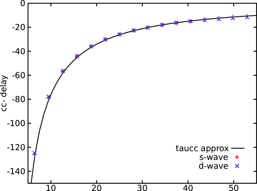
Figure 1: Continuum–continuum delay, $\tau_{cc}(l_{f})$, extracted from two-photon matrix elements for absorption and emission of IR photons on particular partial wave paths leading to $l_{f}$ from the helium ground state. The black line the corresponding $\tau_{cc}(l_{f})$ of hydrogen [Dahlstrom201353].

For angle-resolved delays, however, the relative phases of the $(+)$ and $(-)$ processes between different final partial wave angular states is important because these different final states will interfere. This is clear from the explicit form of a momentum state

$$\psi^{(-)}_{{\bm{k}}}({\bm{r}})=k^{-1/2}\sum\limits_{l=0}^{L_{\rm max}}\sum\limits_{\mu=-l}^{l}i^{l}e^{-i\delta_{l}}Y^{*}_{l\mu}(\hat{\bm{k}})Y_{l\mu}(\hat{\bm{r}})R_{kl}(r)\ ,$$ (9)

where we have applied the ingoing boundary condition. Formally $L_{\rm max}$ extends to infinty in Eq. (9), but in our case with of two photon absorption from the $1s$ state in helium, the momentum state can be truncated at $L_{\rm max}=2$ and $\mu=0$. Using Eq. (4) and Eq. (9) we now construct the complex amplitude for angle-resolved photoelectron by absorption of two photons $\omega_{2q-1}$ and $\omega$

$${\cal M}^{\rm(+)}_{{\bm{k}}_{\bm{f}}}=k_{f}^{-1/2}\sum_{l_{f}=0,2}i^{-l_{f}}e^{i\delta_{f}}Y_{l_{f},0}({\bm{n}}_{\bm{f}})M(f,\omega,\omega_{2q-1},i)\\$$ (10)

and for absorption of one photon $\omega_{2q+1}$ followed by stimulated emission of $\omega$

$${\cal M}^{(\rm-)}_{{\bm{k}}_{\bm{f}}}=k_{f}^{-1/2}\sum_{l_{f}=0,2}i^{-l_{f}}e^{i\delta_{f}}Y_{l_{f},0}({\bm{n}}_{\bm{f}})M(f,-\omega,\omega_{2q+1},i)\\$$ (11)

both leading to the same final state with photoelectron momentum, ${\bm{k}}_{\bm{f}}=k_{f}{\bm{n}}_{\bm{f}}$ with $k_{f}=\sqrt{2\epsilon_{f}}=\sqrt{2(2q\omega+\epsilon_{i})}$. The factor $k_{f}^{-1/2}$ comes from momentum normalization while the states in $M$ are normalized to energy [Starace1982]. The probability for directed photoemission is proportional to

$$S_{2q}({\bm{k}}_{\bm{f}})=2\left|{\cal M}^{(\rm-)}_{{\bm{k}}_{f}}\exp[i(\phi_{2q+1}-\varphi)]+{\cal M}^{(\rm+)}_{{\bm{k}}_{f}}\exp[i(\phi_{2q-1}+\varphi)]\right|^{2},$$ (12)

where we, again, write explicitly the phases of the fields so that the field amplitudes, $E$, inside ${\cal M}$ (and $M$) are real. Eq. (1) and Eq. (2) give the angle-resolved atomic delay

$$\tau_{a}({\bm{k}}_{\bm{f}})=\Delta\theta_{2q}({\bm{k}}_{\bm{f}})/2\omega=\arg[{\cal M}^{(-)}_{{\bm{k}}_{\bm{f}}}{\cal M}^{*(+)}_{{\bm{k}}_{\bm{f}}}]/2\omega,$$ (13)

where, in contrast to the angle-integrated expression (7), the interference of the two final partial waves depends on the direction of the vector ${\bm{k}}_{\bm{f}}$. Results for the angle-resolved atomic delay are given in Sec. 3, where we show that the angular dependence of the time delay can be easily interpreted using LOPT as a competition of the continuum–continuum transitions $Ep\to E^{\prime}d$ and $Ep\to E^{\prime}s$ driven the the IR absorption. As can be expected, this competition may become particularly intense near the geometric node of the $d$-spherical wave.

In the spirit of Dahlstrom201353, we now make a connection between the continuum–continuum delay $\tau_{cc}$, and the corresponding phase-shifts $\phi_{cc}^{(\pm)}$, of the two photon matrix element. We define “exact” $\phi_{cc}^{(+)}(\epsilon_{f}l_{f})$ and $\phi_{cc}^{(-)}(\epsilon_{f}l_{f})$, for absorption and emission of an IR photon to the final state with angular momentum $l_{f}$ with energy $\epsilon_{f}$ as

$$\phi_{cc}^{(+)}(\epsilon_{f}l_{f}) = \arg M^{(+)}_{f}-\frac{\pi}{2}(l_{f}-2)-\delta_{2q-1}+\delta_{f}$$

$$\phi_{cc}^{(-)}(\epsilon_{f}l_{f}) = \arg M^{(-)}_{f}-\frac{\pi}{2}(l_{f}-2)-\delta_{2q+1}+\delta_{f},$$ (14)

where $\delta_{2q-1}$ and $\delta_{2q+1}$ are the atomic scattering phases of the on-shell intermediate $p$-wave and $\delta_{f}$ is that of the final $s$ or $d$-wave. The result is presented in Fig. 2, where we observe that the CC-phases leading to different angular momentum final states differ for low kinetic energy electrons. Comparing with the exact calculation for hydrogen, Fig. 3 in Ref. [Dahlstrom201353], a similar level of discrepancy between the $sps$ and $spd$ angular momentum paths is identified. This shows that the deviations from the approximate continuum–continuum phases arise already in hydrogen and that they do not require any additional short-range interactions (such as correlation effects). The question arises why the CC-delay of the $s$ and $d$-waves are identical, as was shown in Fig. 1, when the CC-phases are obviously different close to threshold. Closer inspection shows that the CC-phases of the $d$-wave are slightly below those of the $s$-wave in both aborption and emission processes by nearly the same amount, say $\phi_{cc}(\epsilon_{f}d)\approx\phi_{cc}(\epsilon_{f}s)-\xi(\epsilon_{f})$. When computing the CC-delay from the CC-phases one takes the difference of emission and absorption processes, $\tau_{cc}(l_{f})=[\phi_{cc}^{(-)}(l_{f})-\phi_{cc}^{(+)}(l_{f})]/2\omega$, so that this constant phase difference cancels.

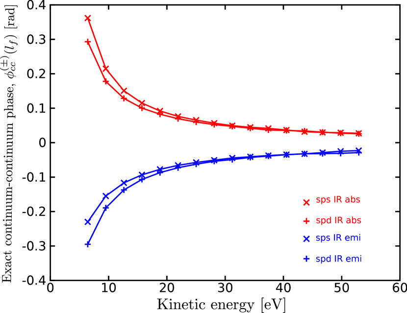
Figure 2: Continuum–continuum phases, for absorption and emission of an IR photon.

2.2 TDSE approach

We solve the TDSE for a helium atom described within a SAE approximation

$$i{\partial\Psi({\bm{r}})/\partial t}=\left[\hat{H}_{\rm atom}+\hat{H}_{\rm int}(t)\right]\Psi({\bm{r}})\ ,$$ (15)

where $\hat{H}_{\rm atom}$ is the Hamiltonian of the field-free atom with an effective one-electron potential [Sarsa2004163]. The Hamiltonian $\hat{H}_{\rm int}(t)$ describes the interaction with the external field and is written in the velocity gauge

$$\hat{H}_{\rm int}(t)={\bm{A}}(t)\cdot\hat{\bm{p}}\ \ ,\ \ {\bm{A}(t)}=-\int_{0}^{t}{\bm{E}(t^{\prime})}\ dt^{\prime}.$$ (16)

As compared to the alternative length gauge, this form of the interaction has a numerical advantage of a faster convergence.

The vector potential of the APT is modeled as the sum of 11 Gaussian pulses of altering polarity shifted by a half of the IR period $T=2\pi/\omega$ :

$$A_{x}(t)=\sum_{n=-5}^{5}(-1)^{n}A_{n}\exp\left(-2\ln 2{(t-nT/2)^{2}\over\tau_{x}^{2}}\right)\cos\Big{[}\omega_{x}(t-nT/2)\Big{]}\ .$$ (17)

The amplitude of each pulse is defined as

$$A_{n}=A_{0}\exp\left(-2\ln 2{(nT/2)^{2}\over\tau_{T}^{2}}\right),$$

where $A_{0}$ is the vector potential amplitude related to the field intensity $I=(\omega^{2}/c^{2})A_{0}^{2}$. The XUV central frequency is $\omega_{x}=1.378$ au $=37.5$ eV. The time constants $\tau_{x}=0.14$ fs and $\tau_{T}=4.83$ fs determine the length of an XUV pulse and the APT train, respectively. The field intensity of the APT is chosen at $5\times 10^{8}~{}\rm W/cm^{2}$ and the XUV frequency $\omega_{x}\simeq 25\omega$.

The vector potential of the IR pulse is modeled by the cosine squared envelope

$$A(t)=A_{0}\cos^{2}\left({\pi(t-\tau)\over 2\tau_{\rm IR}}\right)\cos[\omega(t-\tau)]\ ,$$ (18)

with an intensity of $3\times 10^{11}$ W/cm² and pulse duration of $\tau_{\rm IR}=14.5$ fs. The IR pulse is shifted relative to the APT by a variable delay $0\leq\tau\leq 0.5T$. A positive delay, $\tau>0$, corresponds to the IR pulse being delayed with respect to the center of the XUV pulse train. Further, the laser photon energy is $\omega=0.05841$ au $=1.59$ eV, which corresponds to a period of $T=2\pi/\omega=107$ au = 2.60 fs. The laser pulse duration is $\tau=5.58T=14.5$ fs.

The vector potential of the APT [Eq. (17)] and the IR pulse [Eq. (18)] are visualized on the central panel of Figure 3 along with the squared APT amplitudes $(\omega^{2}/c^{2})A_{n}^{2}$ (left) and the APT spectral content (right).

Figure 3: (Color online) Left: XUV pulses intensity $(\omega^{2}/c^{2})A_{n}^{2}$ (in GW/cm²). The arrow visualizes $\tau_{T}=1.86T=4.83$ fs Center: The vector potentials of the APT (red solid line) and the IR pulse (blue dashed line). Right: spectral representation of the vector-potential. The XUV frequency $\omega_{x}=37.5$ eV is chosen to match the 25st harmonic of $\omega=1.59$ eV. The APT/IR delay $\tau=0$.

To solve the TDSE, we follow the strategy tested in our previous works [dstrong, PhysRevA.87.033407]. The solution of the TDSE is presented as a partial wave series

$$\Psi({\bm{r}},t)=\sum\limits_{l=0}^{L_{\rm max}}f_{l}(r,t)Y_{l0}(\theta,\phi)$$ (19)

with only zero momentum projections retained for the linearly polarized light. The radial part of the TDSE is discretized on the grid with the stepsize $\delta r=0.05$ a.u. in a box of the size $R_{\rm max}=2000$ a.u. The number of partial waves in Eq. (19) was limited to $L_{\rm max}=5$ which ensured convergence in the velocity gauge calculations.

Substitution of the expansion (19) into the TDSE gives a system of coupled equations for the radial functions $f_{l\mu}(r,t)$, describing evolution of the system in time. To solve this system, we use the matrix iteration method [velocity1]. The ionization amplitudes $a({\bm{k}})$ are obtained by projecting the solution of the TDSE at the end of the laser pulse on the set of the ingoing scattering states of the target Hamiltonian (9). Squared amplitudes $|a({\bm{k}})|^{2}$ give the photoelectron spectrum in a given direction $\hat{\bm{k}}$ determined by the azimuthal angle $\theta_{k}$. Examples of such spectra in the $\hat{\bm{z}}$ direction $\theta_{k}=0$ and $\theta_{k}=60^{\circ}$ are shown in Figure 4

Figure 4: (Color online) The photoelectron spectra detected at the angles $\theta_{k}=0^{\circ}$ (left) and $\theta_{k}=60^{\circ}$ (right)

This procedure is then repeated for various time delays $\tau$ between the APT and IR fields and the SB intensity oscillations is fitted to Eq. (1) for angle-resolved photoelectrons. After collecting the photoelectron spectra from TDSE in various directions, the SB intensity oscillation with the variable time delay between the APT and IR fields is fitted with the cosine function

$$S_{2q}({{\bm{k}}_{f}})=A+B\cos[2\omega\tau-C]$$ (20)

using the non-linear Marquardt-Levenberg algorithm. The quality of the fit is very good with the errors in all three parameters not exceeding 1%. Several examples of the fit for the SB20 at the photoelectron detection angles $\theta_{k}=0^{\circ}$, $60^{\circ}$ and $90^{\circ}$ are shown in Figure 5.

Figure 5: (Color online) The SB20 intensity oscillation as a function of the time delay $\Delta/T$ for the photoelectron detection angles $\theta_{k}=0^{\circ}$, $60^{\circ}$ and $90^{\circ}$

Figure 6: (Color online) Angular dependence of the fitting parameters $A$, $B$, and $C$ for the SB20. The TDSE and LOPT calculations are shown with the filled (red) circles and open (blue) circles, respectively. The LOPT calculation is normalized to the TDSE in the maximum of the $A$ parameter. The insets show the variation of the $A$ and $B$ parameters near $90^{\circ}$.

3 Results

In this section we compare the results from our frequency-domain and time-domain calculations. The angular dependence of parameters $A$, $B$ and $C$ of Eq. (20) for the SB20 is shown in Figure 6 along with the equivalent set of data from the LOPT calculation. The LOPT $A$-parameter is normalized to the same parameter in the TDSE calculation. This normalization is then kept for the $B$-parameter. The $C$ parameter is plotted on the absolute scale. All the three parameters agree well between the TDSE and LOPT calculations. We note that even the change of sign of the $B$ parameter near $90^{\circ}$, visible on the inset of the middle panel, is reproduced by both calculations.

The group delay $\tau_{\rm GD}$ of the ATP is zero in our approach since we consider Fourier limited attosecond pulses by setting $\phi_{2q+1}=0$, for all integers $q$ in the frequency comb. Hence the parameter $C$ can be converted directly into the atomic time delay as $\tau_{a}=C/2\omega$ according to Eq. (1). The atomic time delay obtained in this fashion is given in Table 1 for the direction along the polarization of the field, which we refer to as the zero angle for photoemission. Again the agreement between the two calculations is good. To connect with Eq. (3) we also show the breakdown of the atomic delay into the Wigner time delay $\tau_{W}$, which was computed separately by a one-photon RPAE program [PhysRevA.87.063404], and the extracted continuum–continuum delay $\tau_{cc}$. Finally we compare the extracted CC term with that of earlier exact calculations in hydrogen [Dahlstrom201353]. The discrepancy between the two CC quantities is reasonably small, less than ten attoseconds. The variation of the atomic time delay relative to the zero angle polarization direction $\Delta\tau=\tau_{a}(\theta_{k})-\tau(0^{\circ})$ is displayed in Figure 7 for SB 18 to 24.

Table 1: Atomic time delay $\tau_{a}$ and its various components $\tau_{W}$ and $\tau_{cc}$ in the $\hat{\bm{z}}$ direction for various side bands.

SB	$n\omega$	$E$	$\tau_{a}$ (as)		$\tau_{W}$ (as)	$\tau_{cc}$ (as)
$n$	eV	eV	TDSE	LOPT	RPAE	[1]	[2]
18	27.9	3.3	-85	-93	231	-324	-315
20	31.0	6.4	-61	-63	60	-123	-129
22	34.1	9.5	-46	-48	30	-78	-83
24	37.2	12.6	-37	-37	16	-53	-57

[1] Atomic delay minus Wigner delay
[2] Fit to exact hydrogen calculation by Richard Taïeb [Dahlstrom201353]

Figure 7: (Color online) Variation of the time delay relative to the zero angle $\Delta\tau_{a}=\tau_{a}(\theta_{k})-\tau_{a}(0^{\circ})$ for SB 18, 20 (top) and SB 22, 24 (bottom). The TDSE results are shown with the (green) asterisks. The LOPT calculations are displayed with the (blue) open circles. The experimental data by 2015arXiv150308966H are visualized with filled circles and error bars.

Figure 8: Fitting the angular variation of the amplitude parameters $A$ and $B$ and the time delay $\Delta\tau_{a}$ with Eq. (24) for SB 20. The (red) filled circles display the TDSE calculation whereas the thick solid line visualize the fit. The restricted set of fitting parameters with $\phi^{\pm}_{ds}=0$ is represented by the blue dashed line whereas the $\cos^{4}\theta$ fit to the $A$ and $B$ parameters is displayed with the (purple) dotted line.

To highlight the competition between the $s$ and $d$-channels in two-photon ionization into the direction ${\bm{n}}_{\bm{f}}$, we parametrize the absorption and emission amplitudes Eq. (10) and Eq. (11) in the form suggested in 2015arXiv150308966H:

$${\cal M}^{(\pm)}_{{\bm{k}}_{\bm{f}}}\propto 1+c_{ds}^{(\pm)}e^{i\phi_{ds}^{(\pm)}}\sqrt{4\pi}Y_{20}({\bm{n}}_{\bm{f}})\ \ ,\ \$$ (21)

where

$$c_{ds}^{(\pm)}=|M_{d}^{(\pm)}/M_{s}^{(\pm)}|$$ (22)

and

$$\phi_{ds}^{(\pm)}=\arg[(i^{-2}e^{i\delta_{d}}M_{d}^{(\pm)})/(i^{-0}e^{i\delta_{s}}M_{s}^{(\pm))})$$ (23)

are the amplitude ratio and phase difference between the $d$ and $s$ partial wave amplitudes of the absorption $(+)$ and emission $(-)$ processes, respectively. Using Eq. (21), the $A$ and $B$ parameters and the angular variation of the atomic time delay $\Delta\tau_{a}$ can be presented as

$$A \propto \left|1+c_{ds}^{(-)}e^{i\phi_{ds}^{(-)}}\sqrt{4\pi}Y_{20}({\bm{n}}_{\bm{f}})\right|^{2}+\left|1+c_{ds}^{(+)}e^{i\phi_{ds}^{(+)}}\sqrt{4\pi}Y_{20}({\bm{n}}_{\bm{f}})\right|^{2}$$ (24)

$$B \propto 2{\rm Re}\left\{\Big{[}1+c_{ds}^{(-)}e^{i\phi_{ds}^{(-)}}\sqrt{4\pi}Y_{20}({\bm{n}}_{\bm{f}})\Big{]}\Big{[}1+c_{ds}^{(+)}e^{i\phi_{ds}^{(+)}}\sqrt{4\pi}Y_{20}({\bm{n}}_{\bm{f}})\Big{]}^{*}\right\}$$

$$\Delta\tau_{a} = {1\over 2\omega}\arg\left\{\Big{[}1+c_{ds}^{(-)}e^{i\phi_{ds}^{(-)}}\sqrt{4\pi}Y_{20}({\bm{n}}_{\bm{f}})\Big{]}\Big{/}\Big{[}1+c_{ds}^{(+)}e^{i\phi_{ds}^{(+)}}\sqrt{4\pi}Y_{20}({\bm{n}}_{\bm{f}})\Big{]}\right\}.$$

Next, we fit the angular variation of the time delay $\Delta\tau_{a}$ from the TDSE calculation using the bottom line of Eq. (24) with $c_{ds}^{(\pm)}$ and $\phi_{ds}^{(\pm)}$ as fitting parameters. The result of this fitting procedure are illustrated in Figure 8 for SB 20. For comparison we also plot the case where we manually set $\phi_{ds}^{(\pm)}=0$ so that all paths have the same phase. While this approximation has negligible effect on the amplitude parameters $A$ and $B$, the atomic delay changes from a smooth step function, which drops from $0$ as at $60^{\circ}$ to $-550$ as close to $90^{\circ}$, to a discrete step that occurs close to 75^∘.

It follows from the soft photon approximation (SPA) [Maquet2007] that the angular dependence of the $A$ and $B$ parameters are simple $\cos^{4}\theta$ functions for an initial $s$-state,

$$B\propto{\rm Re}\left[{\cal M}^{(-)}_{{\bm{k}}_{\bm{f}}}{\cal M}^{*(+)}_{{\bm{k}}_{\bm{f}}}\right] \propto |J_{1}({\bm{\alpha}}_{0}\cdot{\bm{k}}_{f})|^{2}|\langle f|z|i\rangle|^{2}\propto\cos^{4}\theta\ .$$

Here we made a linear approximation to the Bessel function as the parameter ${\bm{\alpha}}_{0}={\bm{F}}_{0}/\omega^{2}$ is small in a weak IR field. This simple dependece fits very well both the $A$ and $B$ parameters. The only deviation occurs at large angles where the $B$ parameter becomes negative while $\cos^{4}\theta$ always remains positive. However, the SPA predicts no angular variation of the time delay. So, angular dependent time delay and alterantion of sign of the $B$ parameter are both signs of breakdown of the SPA.

Numerical values of the $c_{ds}^{(\pm)}$ and $\phi^{(\pm)}_{ds}$ parameters for SB 20 and 22 are shown in Table 2 along with the LOPT calculation and the fully ab initio TDSE calculation [Argenti2014]. The latter TDSE calculation is not restricted by the SAE and the two electrons in the He atom are treated on the equal footing. Agreement between all the three calculations is fairly good. We find that $\phi_{ds}^{(\pm)}$ is small and that it tends to decrease with the energy of the photoelectron (side band order). This is in qualitative agreement with the earlier work on the atomic delay [Dahlstrom201353], where it was found that no phase difference was expected for sufficiently energetic electrons. Here, we study photoelectrons close to the ionization threshold and effects beyond the asymptotic approximation are at play.

Table 2: Numerical values of the fitting parameters $c_{ds}^{(\pm)}$ and $\phi^{(\pm)}_{ds}$ for SB 20 and 22 from the present TDSE-SAE calculation, fully ab initio TDSE calculation by Argenti2014 and the LOPT calculation

	SB 20   tdse			SB 22   tdse
Parameter	sae	ab initio	lopt	sae	ab initio	lopt
$c_{ds}^{(+)}$	1.168	1.174	1.15	1.093	1.098	1.08
$c_{ds}^{(-)}$	0.633	0.677	0.69	0.722	0.685	0.73
$-\phi_{ds}^{(+)}$	0.090	0.082	0.061	0.043	0.056	0.033
$-\phi_{ds}^{(-)}$	0.074	0.076	0.056	0.040	0.047	0.031

The amplitude ratio $c_{ds}^{(\pm)}$ is rather close to unity, which means that the relative weight of the $d$ and $s$ channels in the two-photon ionization process is approximately equal. This demonstrates that Fano’s propencity rule is not applicable for transitions in the continuum. Although not shown in Table 2, the LOPT calculation shows that the amplitude ratio for much higher energies numerically approaches the kinematic limit of $\sqrt{4/5}\approx 0.89$. This high-energy limit indicates that the absorption and emission processes become equal in magnitude and that they have no relative phase difference. The Fano propencity rule does not hold for the second photon as the magnitude of the amplitude ratio is smaller than one.

4 Conclusion

In the present work we studied the angular variation of the atomic time delay in the RABBIT measurement on the helium atom. We applied the non-perturbative TDSE method along with the lowest order perturbation theory with respect to the electron-photon interaction. Our results are compared favourably with the recent COLTRIMS measurement by 2015arXiv150308966H.

In the experimentally accessible angular range of 0 to $65^{\circ}$, where the RABBITT signal is sufficiently strong, the angular variation of the time delay is rather small. Only SB18 displays a noticeable angular variation of about 60 as. The time delay on other side bands remain flat in this angular range. Given the rapid drop of the magnitude $A$ and $B$ parameters in Eq. (1) with the detection angle as $\cos^{4}\theta$, the angular averaged time delay $\bar{\tau}_{a}$ will be very close to that recorded in the polarization direction of light at the zero degree angle $\tau_{a}(\theta=0)$ . This allows to use the helium atom as a convenient standard both in the angular specific streaking and angular averaged RABBITT time delay measurements.

The partial wave analysis indicates that the $d$ and $s$ channels are equally important in the two-photon ionization continuum both for the angular variation of the magnitude $A$ and $B$ parameters as well as the atomic time delay $\tau_{a}$ in the whole angular range. This is contrary to the intuitive assumption that the $d$ wave normally outweighs the $s$ wave and their competition becomes noticeable only beyond the magic angle. The parametrization with the modulus ratio of the $s$ and $d$ ionization amplitudes and their relative phase in the absorption and emission channels provides a convenient tool to analyze influence of various factors on the RABBITT signal. It also allows to make a quantitative comparison between various calculations. Unfortunately, the statistics of the experimental data [2015arXiv150308966H] is insufficient to extract these parameters and to compare with theoretical predictions. We hope that this statistics will improve in the future to facilitate such a comparison.

We also intend to apply this analysis to the angular variation of time delay in heavier noble gas atoms, Ne and Ar, as well as in the hydrogen molecule. The asymptotic properties of the two-photon ionization amplitude and the atomic time delay hold in this case as well provided there is a strongly dominant single-photon transition $l_{i}\to\lambda$ from the initial state. According to the propensity rule [PhysRevA.32.617], the dipole transition with the increased momentum $l=l_{i}+1$ is usually dominant unless the dominant channel passes through the Coopers minimum. The molecular case introduces an additional degree of freedom of orientation of the inter-nuclear axis. Hence the physics of the angular dependent time delay becomes significantly richer. This work is in progress now [2016arXiv160404938S].

References

References

- [1] \harvarditemAymar \harvardand Crance1980Aymar1980 Aymar M \harvardand Crance M 1980 Two-photon ionisation of atomic hydrogen in the presence of one-photon ionisation Journal of Physics B: Atomic and Molecular Physics 13(9), L287
- [2] \harvarditemCavalieri et al2007cavalieri:07 Cavalieri A L, Müller N, Uphues T, Yakovlev V S, Baltuška A, Horvath B, Schmidt B, Blümel L, Holzwarth R, Hendel S, Drescher M, Kleineberg U, Echenique P M, Kienberger R, Krausz F \harvardand Heinzmann U 2007 Attosecond spectroscopy in condensed matter Nature 449, 1029–1032
- [3] \harvarditemDahlström et al2013Dahlstrom201353 Dahlström J M, Guénot D, Klünder K, Gisselbrecht M, Mauritsson J, L.Huillier A, Maquet A \harvardand Taïeb R 2013 Theory of attosecond delays in laser-assisted photoionization Chem. Phys. 414, 53 – 64
- [4] \harvarditemDahlström \harvardand Lindroth2014Dahlstrom2014 Dahlström J M \harvardand Lindroth E 2014 Study of attosecond delays using perturbation diagrams and exterior complex scaling J. Phys. B 47(12), 124012
- [5] \harvarditemFano1985PhysRevA.32.617 Fano U 1985 Propensity rules: An analytical approach Phys. Rev. A 32, 617–618
- [6] \harvarditemGalán \harvardand Argenti2014Argenti2014 Galán A J \harvardand Argenti L 2014. Private communication
- [7] \harvarditemGuénot et al2012PhysRevA.85.053424 Guénot D, Klünder K, Arnold C L, Kroon D, Dahlström J M, Miranda M, Fordell T, Gisselbrecht M, Johnsson P, Mauritsson J, Lindroth E, Maquet A, Taïeb R, L’Huillier A \harvardand Kheifets A S 2012 Photoemission-time-delay measurements and calculations close to the 3-ionization-cross-section minimum in Ar Phys. Rev. A 85, 053424
- [8] \harvarditemGuénot et al20140953-4075-47-24-245602 Guénot D, Kroon D, Balogh E, Larsen E W, Kotur M, Miranda M, Fordell T, Johnsson P, Mauritsson J, Gisselbrecht M, Varjù K, Arnold C L, Carette T, Kheifets A S, Lindroth E, L’Huillier A \harvardand Dahlström J M 2014 Measurements of relative photoemission time delays in noble gas atoms J. Phys. B 47(24), 245602
- [9] \harvarditemHentschel et al2001HentschelNature2001 Hentschel M, Kienberger R, Spielmann C, Reider G A, Milosevic N, Brabec T, Corkum P, Heinzmann U, Drescher M \harvardand Krausz F 2001 Attosecond metrology Nature 414, 509 – 513
- [10] \harvarditemHeuser et al20152015arXiv150308966H Heuser S, Jiménez Galán Á, Cirelli C, Sabbar M, Boge R, Lucchini M, Gallmann L, Ivanov I, Kheifets A S, Dahlström J M, Lindroth E, Argenti L, Martín F \harvardand Keller U 2015 Time delay anisotropy in photoelectron emission from the isotropic ground state of helium ArXiv e-prints 1503.08966, Nat. Phys. submitted
- [11] \harvarditemItatani et al2002ItataniPRL2002 Itatani J, Quéré F, Yudin G L, Ivanov M Y, Krausz F \harvardand Corkum P B 2002 Attosecond streak camera Phys. Rev. Lett. 88, 173903
- [12] \harvarditemIvanov2011dstrong Ivanov I A 2011 Time delay in strong-field photoionization of a hydrogen atom Phys. Rev. A 83(2), 023421
- [13] \harvarditemIvanov \harvardand Kheifets2013PhysRevA.87.033407 Ivanov I A \harvardand Kheifets A S 2013 Time delay in atomic photoionization with circularly polarized light Phys. Rev. A 87, 033407
- [14] \harvarditemKheifets2013PhysRevA.87.063404 Kheifets A S 2013 Time delay in valence-shell photoionization of noble-gas atoms Phys. Rev. A 87, 063404
- [15] \harvarditemKlünder et al2011PhysRevLett.106.143002 Klünder K, Dahlström J M, Gisselbrecht M, Fordell T, Swoboda M, Guénot D, Johnsson P, Caillat J, Mauritsson J, Maquet A, Taïeb R \harvardand L’Huillier A 2011 Probing single-photon ionization on the attosecond time scale Phys. Rev. Lett. 106(14), 143002
- [16] \harvarditemKrausz \harvardand Ivanov2009krausz:rmp:09 Krausz F \harvardand Ivanov M 2009 Attosecond physics Rev. Mod. Phys. 81, 163–234
- [17] \harvarditemMairesse \harvardand Quéré2005MairessePRA2005 Mairesse Y \harvardand Quéré F 2005 Frequency-resolved optical gating for complete reconstruction of attosecond bursts Phys. Rev. A 71, 011401
- [18] \harvarditemMaquet \harvardand Taïeb2007Maquet2007 Maquet A \harvardand Taïeb R 2007 Two-colour ir+xuv spectroscopies: the soft-photon approximation J. Modern Optics 54(13-15), 1847–1857
- [19] \harvarditemMuller2002MullerAPB2002 Muller H 2002 Reconstruction of attosecond harmonic beating by interference of two-photon transitions Applied Physics B: Lasers and Optics 74, s17–s21. 10.1007/s00340-002-0894-8
- [20] \harvarditemNurhuda \harvardand Faisal1999velocity1 Nurhuda M \harvardand Faisal F H M 1999 Numerical solution of time-dependent Schrödinger equation for multiphoton processes: A matrix iterative method Phys. Rev. A 60(4), 3125–3133
- [21] \harvarditemPalatchi et al20140953-4075-47-24-245003 Palatchi C, Dahlström J M, Kheifets A S, Ivanov I A, Canaday D M, Agostini P \harvardand DiMauro L F 2014 Atomic delay in helium, neon, argon and krypton J. Phys. B 47(24), 245003
- [22] \harvarditemPaul et al2001PaulScience2001 Paul P M, Toma E S, Breger P, Mullot G, Augé F, Balcou P, Muller H G \harvardand Agostini P 2001 Observation of a train of attosecond pulses from high harmonic generation Science 292(5522), 1689–1692
- [23] \harvarditemPazourek et al2013C3FD00004D Pazourek R, Nagele S \harvardand Burgdorfer J 2013 Time-resolved photoemission on the attosecond scale: opportunities and challenges Faraday Discuss. 163, 353–376
- [24] \harvarditemPazourek et al2015RevModPhys.87.765 Pazourek R, Nagele S \harvardand Burgdörfer J 2015 Attosecond chronoscopy of photoemission Rev. Mod. Phys. 87, 765
- [25] \harvarditemSarsa et al2004Sarsa2004163 Sarsa A, Gálvez F J \harvardand Buendia E 2004 Parameterized optimized effective potential for the ground state of the atoms He through Xe Atomic Data and Nuclear Data Tables 88(1), 163 – 202
- [26] \harvarditemSchoun et al2014PhysRevLett.112.153001 Schoun S B, Chirla R, Wheeler J, Roedig C, Agostini P, DiMauro L F, Schafer K J \harvardand Gaarde M B 2014 Attosecond pulse shaping around a Cooper minimum Phys. Rev. Lett. 112, 153001
- [27] \harvarditemSchultze et al2010SchultzeScience2010 Schultze M, Fiess M, Karpowicz N, Gagnon J, Korbman M, Hofstetter M, Neppl S, Cavalieri A L, Komninos Y, Mercouris T, Nicolaides C A, Pazourek R, Nagele S, Feist J, Burgdörfer J, Azzeer A M, Ernstorfer R, Kienberger R, Kleineberg U, Goulielmakis E, Krausz F \harvardand Yakovlev V S 2010 Delay in photoemission Science 328, 1658–1662
- [28] \harvarditemSerov \harvardand Kheifets20162016arXiv160404938S Serov V V \harvardand Kheifets A S 2016 Angular anisotropy of time delay in XUV/IR photoionization of H ArXiv e-print 1604.04938
- [29] \harvarditemStarace1982Starace1982 Starace A F 1982 Vol. XXX1 of Springer Handbook of Atomic, Molecular, and Optical Physics Springer Berlin, Heidelberg pp. 1–121
- [30] \harvarditemToma \harvardand Muller2002TomaJPB2002 Toma E S \harvardand Muller H G 2002 Calculation of matrix elements for mixed extreme-ultraviolet–infrared two-photon above-threshold ionization of argon Journal of Physics B: Atomic, Molecular and Optical Physics 35(16), 3435
- [31] \harvarditemWätzel et al20150953-4075-48-2-025602 Wätzel J, Moskalenko A S, Pavlyukh Y \harvardand Berakdar J 2015 Angular resolved time delay in photoemission J. Phys. B 48(2), 025602
- [32] \harvarditemZhang \harvardand Thumm2011PhysRevA.84.033401 Zhang C H \harvardand Thumm U 2011 Streaking and Wigner time delays in photoemission from atoms and surfaces Phys. Rev. A 84, 033401
- [33]