Minimum output entropy of a non-Gaussian quantum channel

Abstract

We introduce a model of non-Gaussian quantum channel that stems from the combination of two physically relevant processes occurring in open quantum systems, namely amplitude damping and dephasing. For it we find input states approaching zero output entropy, while respecting the input energy constraint. These states fully exploit the infinite dimensionality of the Hilbert space. Upon truncation of the latter, the minimum output entropy remains finite and optimal input states for such a case are conjectured thanks to numerical evidences.

I Introduction

Recently the subject of quantum channels has catalysed the attention for its usefulness in foundational issues as well as in technological applications (for a recent review, see CGLM14 ). Formally a quantum channel is a completely positive and trace preserving map acting on the set of states (density operators) living in a Hilbert space. Since any physical process involves a state change, it can be regarded as a quantum channel mapping the initial (input) state to the final (output) state. As such it can be characterized in terms of its information transmission capability. This implies the use of entropic functionals among which the minimum output entropy plays a dominant role. In fact it is related to the minimum amount of noise inherent to the channel, since it quantifies the minimum uncertainty occurring at the output of a channel when inputting pure states. More precisely, the output entropy measures the entanglement of the input pure state with the environment. Being this latter not accessible, such entanglement induces loss of quantum coherence and thus injection of noise at the channel output. Clearly, low values of entanglement, i.e., of output entropy, correspond to low communication noise. As a consequence, the study of output entropy yields useful insights about channel capacities. In particular, an upper bound on the classical capacity can be derived from a lower bound on the output entropy of multiple channel uses King .

When studying quantum channels a dichotomy between discrete and continuous channels usually appears. The formers act on states living in finite dimensional Hilbert space. In contrast the latter act on states living in infinite dimensional Hilbert space. This is reflected in the possibility of using discrete or continuous variables where to encode classical information. Among continuous quantum channels attention has been almost exclusively devoted to Gaussian quantum channels, that is channels mapping Gaussian input states into Gaussian output ones Oleg . The reason is that they are easily implementable at experiment level and moreover they also handy at theoretical level. For these channels the minimum output entropy was largely investigated Vittorio1 and then showed that actually their classical capacity is achieved through states minimizing the output entropy Vittorio2 .

Here, we go beyond the restriction of Gaussianity of continuous quantum channels and propose a model of non-Gaussian quantum channel that stems from the combination of two physically relevant processes that occur in open quantum systems, namely amplitude damping and dephasing. We then analytically find input states approaching zero output entropy, while respecting the input energy constraint. They consist in the superposition of two number states the farthest away one from the other. In truncated Hilbert space, we find that beside superposition of two number states, the so-called binomial states binomial can be optimal depending on the value of channels parameters. We support this latter results by numerical investigations.

The paper is organized as follows. In Section II we introduce the model and then we show the existence of optimal input states achieving zero output entropy in Section III. Subsequently, in Section IV, we restrict our attention to truncated Hilbert space and we conjecture about the optimality of binomial states, beside superposition of two number states, and we give numerical evidences of this idea. Section V is for concluding remarks.

II The model

Let us start considering the Hilbert space $L^{2}(\mathbb{R})$ associated to a single bosonic mode with ladder operator $a,a^{\dagger}$.

In the framework of dynamical maps, a typical example of Gaussian process is provided by the amplitude damping effect described by the master equation openq

$$\frac{d}{dt}\varrho=2a\varrho a^{{\dagger}}-a^{\dagger}a\varrho-\varrho a^{\dagger}a=:\mathcal{L}_{AD}(\varrho),$$

for the density operator $\varrho$. In contrast, a typical example of non-Gaussian process is provided by the purely dephasing effect described by the master equation openq

$$\frac{d}{dt}\varrho=2a^{\dagger}a\varrho a^{\dagger}a-(a^{\dagger}a)^{2}\varrho-\varrho(a^{\dagger}a)^{2}=:\mathcal{L}_{PD}(\varrho).$$

In order to interpolate between these two regimes we are going to consider the following dynamics

$$\frac{d}{dt}\varrho=(1-\epsilon)\mathcal{L}_{AD}(\varrho)+\epsilon\mathcal{L}_{PD}(\varrho),$$ (1)

with $\epsilon\in[0,1]$. It is easy to see that

$$\mathcal{L}_{AD}(\mathcal{L}_{PD}(\varrho))=\mathcal{L}_{PD}(\mathcal{L}_{AD}(\varrho)).$$

Therefore we can write the formal solution of (1) as

$$\varrho(t)=e^{(1-\epsilon)t\mathcal{L}_{AD}}e^{\epsilon t\mathcal{L}_{PD}}\varrho(0).$$ (2)

Actually this map can be regarded as a quantum channel $\Phi_{\epsilon,t}$ (depending on the parameters $\epsilon$ and $t$) mapping

$$\varrho(0)\mapsto\varrho(t)=\Phi_{\epsilon,t}(\varrho(0))=\sum_{j,k=0}^{\infty}E_{jk}\varrho(0)E_{jk}^{\dagger},$$ (3)

where $E_{jk}$ are the Karus operators CGLM14 . In view of (2)

$$E_{jk}=A_{j}P_{k},$$

where $A_{j}$ are the amplitude damping Kraus operators Liu04

$$A_{j}=\sum_{l=j}^{\infty}\sqrt{l\choose j}\left[1-f(\epsilon,t)\right]^{(l-j)/2}\left[f(\epsilon,t)\right]^{j/2}|l-j\rangle\langle l|,$$ (4)

with $f(\epsilon,t):=1-e^{-2(1-\epsilon)t}$, and $P_{k}$ are the phase damping Kraus operators Liu04

$$P_{k}=\sum_{l=0}^{\infty}\sqrt{\frac{(2l^{2}\epsilon t)^{k}}{k!}}e^{-l^{2}\epsilon t}|l\rangle\langle l|.$$ (5)

In Eqs.(4) and (5) it is used the Fock basis $\{|l\rangle\}_{l\in\mathbb{N}_{0}}$ representation. Expanding $\varrho(0)$ in the same basis as $\varrho(0)=\sum_{m,n=0}^{\infty}C_{m,n}(0)|m\rangle\langle n|$ and considering the channel in (3), we obtain

$$\varrho(t)=\sum_{m,n=0}^{\infty}C_{m,n}(t)|m\rangle\langle n|,$$ (6)

with

$$C_{m,n}(t) =e^{-Y_{m,n}(\epsilon)t}$$ (7)

$$\times\sum_{l=0}^{\infty}C_{{}_{m+l,n+l}}(0)\left[{m+l\choose l}{n+l\choose l}\right]^{\frac{1}{2}}f^{l},$$

in which $Y_{m,n}(\epsilon):=(1-\epsilon)(m+n)+\epsilon(m-n)^{2}$. Equation (7) is also the solution of the following recursive relation

$$\dot{C}_{m,n}(t) =2(1-\epsilon)\sqrt{(m+1)(n+1)}C_{m+1,n+1}(t)$$ (8)

$$-Y_{m,n}(\epsilon)C_{m,n}(t),$$

which is obtainable from the master equation (1).

When dealing with quantum channels acting on the set of states living in an infinite dimensional Hilbert space, it is customary to employ the constraint of fixed average input energy, that is

$${\rm Tr}\left(\varrho(0)a^{\dagger}a\right)=N.$$ (9)

III Minimizing output entropy

The output entropy of the quantum channel $\Phi$ in Eq.(3) is the von Neumann entropy of the output state, namely

$$S\left(\Phi_{\epsilon,t}\left(\rho\right)\right):=-{\rm Tr}\left[\Phi_{\epsilon,t}\left(\rho\right)\log_{2}\left(\Phi_{\epsilon,t}\left(\rho\right)\right)\right].$$ (10)

In order to quantify the noise inherent to the quantum channel $\Phi_{\epsilon,t}$ we look for its minimal output entropy and call the state with minimum output entropy the optimal input state.

The following Theorem states the existence of states with zero output entropy.

Theorem 1

Input states

$$|\kappa_{\alpha}\rangle=\sqrt{1-\frac{N}{K}}|0\rangle+\sqrt{\frac{N}{K}}e^{i\alpha K}|K\rangle,\quad K\in\mathbb{N},$$ (11)

with $\alpha\in\mathbb{R}$, respect the input energy constraint (9) and satisfy

$$\lim_{K\to\infty}S\left(\Phi_{\epsilon,t}\left(|\kappa_{\alpha}\rangle\langle\kappa_{\alpha}|\right)\right)=0,$$ (12)

for all values of $\epsilon$ and $t$.

Proof First we note that all the states $|\kappa_{\alpha}\rangle$ have the same output entropy due to the covariance property of the channel under unitary transformations

$$U\in\mathcal{U}:=\bigg{\{}\sum_{n}e^{i\alpha n}|n\rangle\langle n|\,\Big{|}\,\alpha\in\mathbb{R},n\in\mathbb{N}_{0}\bigg{\}}.$$

Therefore, we prove the theorem for $|\kappa_{0}\rangle$. Using Eq.(3), the corresponding output reads

$$\Phi_{\epsilon,t}\left(|\kappa_{0}\rangle\langle\kappa_{0}|\right)=\left(1-\frac{N}{K}(1-f^{K})\right)|0\rangle\langle 0|$$

$$+\sqrt{\frac{N}{K}\left(1-\frac{N}{K}\right)}(1-f)^{K}e^{-\epsilon K^{2}t}\left(|0\rangle\langle K|+|K\rangle\langle 0|\right)$$

$$+\frac{N}{K}\sum_{m=1}^{K}{K\choose m}(1-f)^{m}f^{K-m}|m\rangle\langle m|.$$

The matrix form of this output state is block-diagonal, so the eigenvalues can be easily found as

$$\lambda_{0,K} =\frac{1}{2}\left(A+B\pm\sqrt{(A-B)^{2}+4C^{2}}\right),$$

$$\lambda_{m} =\frac{N}{K}{K\choose m}(1-f)^{m}f^{K-m},\qquad m=1,\ldots,K-1,$$

with

$$A :=1-\frac{N}{K}\left(1-f^{K}\right),$$

$$B :=\frac{N}{K}\left(1-f\right)^{K},$$

$$C :=\sqrt{\frac{N}{K}\left(1-\frac{N}{K}\right)}(1-f)^{K}e^{-\epsilon K^{2}t}.$$

It is easy to see that all the eigenvalues approach zero for $K\rightarrow\infty$, except $\lambda_{0}$ that approaches one. Therefore the input state (11), while satisfying the input energy constraint, leads to a zero output entropy. More precisely, its output entropy results:

$$S\left(\Phi_{\epsilon,t}\left(|\kappa_{0}\rangle\langle\kappa_{0}|\right)\right)=-\lambda_{0}\log_{2}\lambda_{0}-\lambda_{K}\log_{2}\lambda_{K}$$

$$-\frac{N}{K}\left[1-f^{K}-(1-f)^{K}\right]\log_{2}\left(\frac{N}{K}\right)$$

$$+\frac{N}{K}\left[f^{K}\log_{2}(f^{K})+(1-f)^{K}\log_{2}\left((1-f)^{K}\right)\right]$$

$$+\frac{N}{K}\frac{1}{2}\log_{2}\left(2\pi eKf(1-f)\right)+{\cal O}\left(\frac{1}{K}\right).$$ (13)

Now fixing $\mathcal{E}>0$ we should find $\mathcal{K}\in\mathbb{N}$ such that $S\left(\Phi_{\epsilon,t}\left(|\kappa_{0}\rangle\langle\kappa_{0}|\right)\right)<\mathcal{E}$ for $K>\mathcal{K}$. To this end we first find an upper bound for (III). Since projective measurements increase entropy MOhya , we have the inequality

$$S\left(\Phi_{\epsilon,t}\left(|\kappa_{0}\rangle\langle\kappa_{0}|\right)\right)\leq H\left(p_{\epsilon,t}(n)\right)$$

where the r.h.s. is the Shannon entropy of the probability mass function $p_{\epsilon,t}(n):=\langle n|\Phi_{\epsilon,t}\left(|\kappa_{0}\rangle\langle\kappa_{0}|\right)|n\rangle$. Explicitly the latter reads

$$p_{\epsilon,t}(n)=\left\{\begin{array}[]{ccc}1-\frac{N}{K}(1-f^{K})&&n=0\cr\cr\frac{N}{K}{K\choose n}(1-f)^{m}f^{K-n}&&n=1,\ldots,K\end{array}\right..$$

As a consequence

$$H\left(p_{\epsilon,t}(n)\right) =-\left[1-\frac{N}{K}\left(1-f^{K}\right)\right]\log_{2}\left[1-\frac{N}{K}\left(1-f^{K}\right)\right]$$

$$-\frac{N}{K}\log_{2}\left(\frac{N}{K}\right)+\frac{N}{K}f^{K}\log_{2}\left(\frac{N}{K}f^{K}\right)$$

$$+\frac{1}{2}\frac{N}{K}\log_{2}\left(2\pi eKf(1-f)\right)+{\cal O}\left(\frac{1}{K}\right).$$

Using the inequality $-x\log x<\sqrt{x(1-x)}$ we then get

$$H\left(p_{\epsilon,t}(n)\right) \leq\sqrt{\left(1-\frac{N}{K}\left(1-f^{K}\right)\right)\frac{N}{K}\left(1-f^{K}\right)}$$

$$+\sqrt{\frac{N}{K}\left(1-\frac{N}{K}\right)}+\frac{1}{2}\frac{N}{K}\sqrt{2\pi eKf\left(1-f\right)}$$

$$\leq 2\sqrt{\frac{N}{K}}+\sqrt{\frac{N}{K}\frac{\pi}{2}eNf(1-f)}.$$

By imposing that the above r.h.s. becomes smaller than $\mathcal{E}$, it follows

$$\mathcal{K}=\left\lceil\frac{N}{{\cal E}^{2}}\left(2+\sqrt{\frac{\pi}{2}eNf(1-f)}\right)^{2}\right\rceil.$$

IV Space Truncation

In the previous Section we showed that the input states (11) give zero output entropy for $K\rightarrow\infty$. However, if we truncate the Hilbert space to a finite value of $K$, it is not guaranteed that these states are still optimal. Finding the optimal input state under that condition is the aim of this Section. To start with, we introduce a class of states knows as binomial states binomial

$$|B\rangle_{M,\mu}:=\sum_{n=0}^{M}\beta_{n}|n\rangle,\;\;\;\beta_{n}:=\left[{M\choose n}\mu^{n}(1-\mu)^{M-n}\right]^{\frac{1}{2}},$$ (14)

with parameters $M\in\mathbb{N}$ and $\mu\in[0,1]$. The binomial state (14) reduces to the number state $|0\rangle$ for $\mu=0$ and to the number state $|M\rangle$ for $\mu=1$. In contrast, in the limit $\mu\rightarrow 0$, $M\rightarrow\infty$, and $\mu M=\alpha\in\mathbb{R}$ the binomial state approaches the coherent state $|\alpha\rangle$.

The energy constraint (9) yields the relation

$${\rm Tr}\left(|B\rangle_{M,\mu}\langle B|a^{\dagger}a\right)=M\mu=N.$$

Furthermore, inserting the coefficients $\beta_{n}$ of (14) into (7) we get the explicit expression of the output density operator representation in the Fock basis

$$\Phi_{\epsilon,t}(|B\rangle_{M,\mu}\langle B|)=\sum_{m,n=0}^{M}e^{-Y_{m,n}(\epsilon)t}\left(\frac{\mu}{1-\mu}\right)^{\frac{m+n}{2}}$$

$$\times\sum_{l=0}^{M-\max\{m,n\}}\left[{M\choose m+l}{m+l\choose m}{M\choose n+l}{n+l\choose n}\right]^{\frac{1}{2}}$$

$$\times\left(\mu f\right)^{l}\left(1-\mu\right)^{M-l}|m\rangle\langle n|.$$

Here we numerically evaluate the output entropy for binomial input states with average energy $N$. Once $N$ is fixed we still have the freedom to vary $\mu$ and $M$ in a way that $\mu M=N$. Since $\mu\leq 1$, for fixed $N$, we increase $M$ from $\lceil N\rceil$ to $K$, in order to find the minimum value of $S\left({\Phi_{\epsilon,t}\left(|B\rangle_{M,\mu}\langle B|\right)}\right)$. From here on, when we refer to the binomial state $|B\rangle$, we mean the one which has minimum output entropy among other possible binomial states with average energy $N$.

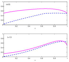
Figure 1: (Color Online) Output entropy for input state $|B\rangle$ (Blue dashed line) and for $|\kappa_{0}\rangle$ (solid magenta line) input states with $N=0.6$ ant $t=0.5$ (top), $t=1.5$ (bottom).

Figure 1 shows the output entropy of the state $|B\rangle$ in (14) (Blue dashed line) and of the state $|\kappa_{0}\rangle$ in (11) (Magenta solid line) versus $\epsilon$ for $N=0.6$ at $t=0.5$ (top) and $t=1.5$ (bottom). Here $4$-dimensional Hilbert space is considered. As can be argued from these figures, the output entropy of $|B\rangle$ remains smaller than the output entropy of $|\kappa_{0}\rangle$ (for any value of $\epsilon$) until $t$ reaches a threshold $t_{*}$. Then, for $t>t_{*}$ the state with less output entropy can be either $|B\rangle$ or $|\kappa\rangle$ depending on the value of $\epsilon$ (see also Fig.2).

To have an estimation of $t_{*}$, we first point out that our numerical analysis shows that the output entropy of $|B\rangle$ and $|\kappa_{0}\rangle$ cross each other at large values of $\epsilon$ where the optimal value of $M$ is 1. In such a case the output state of $|B\rangle$ lives in a two dimensional subspace and its output entropy turns out to be

$$S_{B} =-\sum_{j=1}^{2}\mu_{j}\log(\mu_{j}),$$

$$\mu_{1,2} :=\frac{1\pm\sqrt{(1-2N(1-f))^{2}+4N(1-N)e^{-2t}}}{2}.$$

Then solving the equation $S(\Phi_{\epsilon,t}\left(|\kappa_{0}\rangle\langle\kappa_{0}|)\right)=S_{B},$ we can find the value of $t_{*}$.

To do the similar calculation for any given $N$, we have numerically found that the optimal value of $M$ is $\lceil N\rceil$. Therefore the output entropy of $|B\rangle_{M,\mu}$, with $M=\lceil N\rceil$ and $\mu=N/M$, should be found and equated to $S(\Phi_{\epsilon,t}\left(|\kappa_{0}\rangle\langle\kappa_{0}|)\right)$ in order to get $t_{*}$.

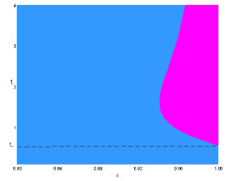
Figure 2: Curve in the $\epsilon,t$ plane where $S(\Phi_{\epsilon,t}(|B\rangle\langle B|))=S(\Phi_{\epsilon,t}(|\kappa_{0}\rangle\langle\kappa_{0}|))$ for $N=0.6$. On the left (resp. on the right) of the curve it is $S(\Phi_{\epsilon,t}(|B\rangle\langle B|))<S(\Phi_{\epsilon,t}(|\kappa_{0}\rangle\langle\kappa_{0}|))$ (resp. $S(\Phi_{\epsilon,t}(|B\rangle\langle B|))>S(\Phi_{\epsilon,t}(|\kappa_{0}\rangle\langle\kappa_{0}|))$). The horizontal dashed line represents the value of $t_{*}$.

After having compared the behaviour of the output entropy for inputs of the kind (11) and (14), we formulate the following conjecture.

Conjecture 1

In a truncated Hilbert space of dimension $K+1$, the minimal output entropy of the quantum channel (3) is achieved either by binomial states of Eq.(14) or by states $|\kappa_{\alpha}\rangle$ of Eq. (11), depending on the values of $\epsilon$ and $t$.

To support this Conjecture we perform a uniform random search over all pure input states in the finite dimensional Hilbert space. The restriction to search only among pure states is motivated by the following Lemmas.

Lemma 1

Given a self adjoint operator $H:\mathbb{C}^{K+1}\to\mathbb{C}^{K+1}$, we can always decompose a density operator $\rho$ on $\mathbb{C}^{K+1}$ satisfying a linear constraint ${\rm Tr}(\rho H)=N$, in terms of pure states $|\psi_{k}\rangle$ satisfying the same constraint, i.e. ${\rm Tr}(|\psi_{k}\rangle\langle\psi_{k}|H)=N$.

Proof Consider the spectral decomposition of $H=\sum\limits_{j}h_{j}|j\rangle\langle j|$. An arbitrary density operator represented in the $H$ eigenvectors basis

$$\rho=\sum\limits_{i,j}r_{i,j}|i\rangle\langle j|,\quad r_{j,j}>0,\quad\sum\limits_{j}r_{j,j}=1,$$ (15)

satisfies the constrain if ${\rm Tr}(\rho H)=\sum\limits_{j}h_{j}r_{{j,j}}=N$. Decomposing $\rho$ in terms of pure states we have

$$\rho=\sum\limits_{k}p_{k}|\psi_{k}\rangle\langle\psi_{k}|,\quad p_{k}>0,\quad\sum\limits_{k}p_{k}=1,$$ (16)

Comparing Eqs.(15) and (16), we find that $\sum\limits_{k}p_{k}|\langle\psi_{k}|j\rangle|^{2}=r_{{j,j}}$. If we take

$$|\langle\psi_{k}|j\rangle|^{2}=r_{{j,j}},\quad\forall k,$$ (17)

it will result

$${\rm Tr}(|\psi_{k}\rangle\langle\psi_{k}|H)=\sum\limits_{j}h_{j}r_{{j,j}}=N,\quad\forall k.$$

Hence it is enough to determine the $|\psi_{k}\rangle$s from the condition (17) to get a decomposition of $\rho$ in terms of pure states satisfying the same constraint. This is always possible, actually in infinite many ways. Additionally we have the freedom in choosing the $p_{k}$s.

Lemma 2

The minimum output entropy of a quantum channel $\Phi$ acting on states $\rho$ on $\mathbb{C}^{K+1}$ satisfying the energy constraint (9) is achieved on pure states.

Proof Assume that the minimum output entropy is achieved by the input state $\rho$ satisfying the energy constraint. Decomposing it in terms of pure states that satisfy the same energy constraint $\rho=\sum_{k}p_{k}|\psi_{k}\rangle\langle\psi_{k}|$, and using the concavity of von Neumann entropy MOhya , we have

$$S(\Phi(\rho)) = S\big{(}\sum_{k}p_{k}\Phi\left(|\psi_{k}\rangle\langle\psi_{k}|\right)\big{)}$$

$$\geq \sum_{k}p_{k}S\left(\Phi\left(|\psi_{k}\rangle\langle\psi_{k}|\right)\right).$$

In the decomposition, let us denote the pure state with minimum output entropy by $|\psi_{*}\rangle$. Therefore we have:

$$S\left(\Phi(\rho)\right)\geq S\left(\Phi\left(|\psi_{*}\rangle\langle\psi_{*}|\right)\right),$$

that is, the optimal input state must be pure.

To generate random pure input states in $K+1$-dimensional Hilbert space, we employ the following parametrization

$$|\psi\rangle =\sum_{n=0}^{K}\nu_{n}|n\rangle,$$

$$\nu_{0} =\cos\theta_{K},\quad\nu_{n>0}=e^{i\phi_{n}}\cos\theta_{K-n}\prod_{l=K-n+1}^{K}\sin\theta_{l}.$$

Then, according to Karol , it is enough to generate $\phi_{n\geq 1}\in[0,2\pi)$ from a uniform distribution $p(\phi_{n\geq 1})=\frac{1}{2\pi}$ and random independent variables $\xi_{n}$ distributed uniformly in $[0,1]$ for $n=1,\ldots,K$ defining

$$\theta_{n}:=\arcsin(\xi_{n}^{\frac{1}{2n}}).$$

However, due to the energy constraint (9), we should consider states satisfying $\sum_{n=0}^{K}n|\nu_{n}|^{2}=N$. This imposes a functional relation among $\theta_{n}$s and so among $\xi_{n}$s, which can be written as: $\xi_{K}=g(\xi_{1},\xi_{2},\ldots\xi_{K-1};N)$. Therefore we should generated $K-1$ random variables with the following modified probability distribution function

$$\tilde{p}(\xi_{1},\ldots,\xi_{K-1})={\cal C}\int d\xi_{K}p(\xi_{1},\ldots,\xi_{K})\delta\left(\xi_{K}-g\right),$$

being ${\cal C}$ a normalization factor and $p(\xi_{1},\ldots,\xi_{K})$ the probability distribution function for the variables $\xi_{1},\ldots,\xi_{K}$. Since these are chosen independently and with a standard uniform distribution in $[0,1]$, we conclude that we should generate $\xi_{1},\ldots,\xi_{K-1}$ according to $\tilde{p}(\xi_{1},\ldots,\xi_{K-1})=p(\xi_{1},\ldots,\xi_{K-1})=1$, and pick $\xi_{K}$ as

$$\xi_{K}=g(\xi_{1},\ldots,\xi_{K-1};N)$$

$$=\frac{N}{\left[1+\xi_{K-1}^{1/{(K-1)}}\left(1+\xi_{K-2}^{1/(K-2)}\left(1+\cdots\xi_{2}^{1/2}\left(1+\xi_{1}\right)\right)\right)\right]}.$$

In our $4$-dimensional example with $N=0.6$ the search over $10^{5}$ states, generated as explained above, confirms the statement of Conjecture 1.

V Conclusion

We have opened an avenue for studying, from an information theoretic point of view, continuous quantum channels beyond the usual restriction of Gaussianity. Actually we have proposed a model of non-Gaussian quantum channel that stems from a master equation accounting for two processes, amplitude damping and dephasing. Its physical relevance relies on the fact that amplitude damping and dephasing are applied in many concrete discussions to model noise of quantum information processing with single mode light field, vibration phonon mode, or excitonic wave, see e.g. Lidar .

Then, the first question that arises is how much the introduced channel deviates from Gaussianity. Arguably this depends on the parameter $\epsilon$, however an exact quantification would be in order, maybe in a fashion similar to what has been done for non-Gaussian states Konrad . This could also shed light on the choice of optimal input states for communication tasks. Here we found input states approaching zero output entropy, while respecting the input energy constraint. They consist in the superposition of two number states the farthest away one from the other. In truncated Hilbert space, the minimum output entropy remains finite and optimal input states are conjectured to be binomial states beside superposition of two number states, depending on the values of the channel’s parameters. This is corroborated by numerical results. The study performed in truncated Hilbert space is justified by the fact that in realistic physical situations is hard to fully exploit the infinite dimensionality of the space $L^{2}(\mathbb{R})$.

As further development one could address the issue of additivity of output entropy for two copies of the channel and then eventually of multiple copies. This would be motivated by the additivity of the classical capacity deriving from the additivity of the minimum output entropy Shor .

Although challenging, the introduced map leaves concrete hopes for characterizing its (product states) classical capacity which implies finding the optimal input ensemble of states maximizing the Holevo chi quantity Holevo .

References

(1)
F. Caruso, V. Giovannetti, C. Lupo, and S. Mancini,
Rev. Mod. Phys. 86, 1203 (2014).
(2)
K. King, IEEE Trans. Inf. Theory 49, 221 (2003);
K. King, and M. B. Ruskai, IEEE Trans. Inf. Theory 47,
192 (2001).
(3)
O. V. Pilyavets, C. Lupo, and S. Mancini,
IEEE Trans. Inf. Theory 58, 6126 (2012).
(4)
V. Giovannetti, A. S. Holevo, S. Lloyd, and L. Maccone,
J. Phys. A: Math. Theor. 43 415305 (2010);
V. Giovannetti, S. Guha, S. Lloyd, L. Maccone, and J. H. ShapiroPhys.
Rev. A 70, 032315 (2004).
(5)
V. Giovannetti, R. Garcia-Patron, N. J. Cerf, and A. S. Holevo,
Nat. Phot. 8, 796 (2014).
(6)
A. V. Barranco, and J. Roversi, Phys. Rev. A 50, 5233
(1994);
C. T. Lee, Phys. Rev. A 31, 1213 (1985);
D. Stoler, B. E. A. Saleh, and M. C. Teich, Opt. Acta.
32, 345 (1985).
(7)
H. P. Breuer, and F. Petruccione, The Theory of Open
Quantum Systems, Oxford University Press, Oxford (2002).
(8)
Y. Liu, S. K. Ozdemir, A. Miranowicz, and N. Imoto,
Phys. Rev. A 70, 042308 (2004).
(9)
M. Oyha, and D. Petz, Quantum Entropy and Its
Use, Springer, Berlin (1993).
(10)
K. Zyczkowski, H.-J. Sommers, J. Phys. A: Math. Theor.
34, 7111 (2001).
(11)
D. A. Lidar, Z. Bihary, and K. B. Whaley, Chem. Phys.
268, 35 (2001);
D. Bacon, D. A. Lidar, and K. B. Whaley, Phys. Rev. A
60, 1944 (1999).
(12)
M. G. Genoni, M. G. A. Paris, and K. Banaszek, Phys. Rev. A
78, 060303 (R), (2008).
(13)
P. W. Shor, Comm. Math. Phys. 246, 453 (2004).
(14)
A. S. Holevo, IEEE Trans. Inf. Theory 44, 269 (1998).