Band-Renormalization Effects and Predominant Antiferromagnetic
Order in Two-Dimensional Hubbard Model

Abstract

Band renormalization effects (BRE) are comprehensively studied for a mixed state of $d_{x^{2}-y^{2}}$-wave superconducting ($d$-SC) and antiferromagnetic (AF) orders, in addition to simple $d$-SC, AF, and normal (paramagnetic) states, by applying a variational Monte Carlo method to a two-dimensional Hubbard ($t$-$t^{\prime}$-$U$) model. In a weakly correlated regime ($U/t\lesssim 6$), BRE are negligible on all the states studied. As previously shown, the effective band of $d$-SC is greatly renormalized but the modifications of physical quantities, including energy improvement, are negligible. In contrast, BRE on the AF state considerably affects various features of the system. Because the energy is markedly improved for $t^{\prime}/t<0$, the AF state occupies almost the whole underdoped regime in phase diagrams. A doped metallic AF state undergoes a kind of Lifshitz transition at $t^{\prime}=t^{\prime}_{\rm L}\sim-0.05t$ as $t^{\prime}/t$ varies, irrespective of the values of $U/t$ and $\delta$ (doping rate). Pocket Fermi surfaces arise around $(\pi,0)$ [$(\pi/2,\pi/2)$] for $t^{\prime}>t^{\prime}_{\rm L}$ [$t^{\prime}<t^{\prime}_{\rm L}$], which corresponds to the electron-hole asymmetry observed in angle-resolved photoemission spectroscopy (ARPES) spectra. The coexistent state of the two orders is possible basically for $t^{\prime}>t^{\prime}_{\rm L}$, because the existence of Fermi surfaces near $(\pi,0)$ is a requisite for the electron scattering of ${\bf q}=(\pi,\pi)$. Actually, the coexistent state appears mainly for $t^{\prime}_{\rm L}/t<t^{\prime}/t\lesssim 0.2$ in the mixed state. Nevertheless, the AF and coexisting states become unstable toward phase separation for $-0.05\lesssim t^{\prime}/t\lesssim 0.2$ but become stable at other values of $t^{\prime}/t$ owing to the energy reduction by the diagonal hopping of doped holes. We show that this instability does not directly correlate with the strength of $d$-SC.

1 Introduction

To clarify the physics of cuprate superconductors (SCs),[1, 2] we have to know the fundamental properties of the $t$-$J$ and Hubbard models on a square lattice with an extension in the kinetic part ($t$-$t^{\prime}$ and $t$-$t^{\prime}$-$t^{\prime\prime}$, etc.) as basic models.[3] In this paper, we mainly focus on the following subjects in the Hubbard ($t$-$t^{\prime}$-$U$) model:

(A) The primary subject is the ground-state phase diagram in the model-parameter space. Although a typical view to date is that the antiferromagnetic (AF) order arising at half filling rapidly vanishes on doping holes and the $d_{x^{2}-y^{2}}$-wave superconductivity ($d$-SC) appears,[3, 4] in accordance with the behavior of cuprates, in recent studies using advanced techniques it was argued that AF orders or inhomogeneous phases prevail in wider ranges of $\delta$ (doping rate).[5, 6, 7]

(B) In phase diagrams of cuprates, the areas of superconducting (SC) and AF phases are in proximity. In the SC phase, appreciable AF correlation or short-range AF orders are observed,[8] but the coexistence of two long-range orders has not been detected except for in multilayered systems. In theory, it is still unclear in what parameter range the two long-range orders coexist and why they are coexisting or mutually exclusive.

(C) Another subject is whether or not homogeneous states are stable against phase separation. Actually, signs of inhomogeneous electronic states or phase separation are often noticed in cuprates such as a stripe structure of charge and spin and a mosaic distribution of the gap magnitude. Theoretically, it is again unclear as to the ranges of $U/t$, $t^{\prime}/t$, and $\delta$ and the cause of the state becoming unstable toward phase separation.

So far, these subjects have been addressed by many researchers with a variety of methods, in particular, dynamical mean field theories (DMFTs) with some extensions [9, 10, 11, 12, 6, 7] and variational Monte Carlo (VMC) methods[13, 14, 15, 16, 17, 18, 19, 20, 4, 5] are useful tools to quantitatively treat strong local correlations. One also needs to consider the effects of antiferromagnetism (AF) because it is crucial even for subject (C). The results regarding (A)-(C) of the above studies do not seem unified but are rather scattered at first glance. Although inconsistencies exist among them, we feel that the main source of confusion resides in insufficient consideration of the difference in the diagonal hopping term ($t^{\prime}$). In most of the above studies, $t^{\prime}/t$ (and $t^{\prime\prime}/t$) was set to specific values, say $0$ and/or $-0.3$, but we are apt to read the results associated with (A)-(C) without care in while also considering the value of $t^{\prime}/t$. If we arrange the results by specifying the value of $t^{\prime}/t$, they are often consistent beyond our expectation, as shown later in Table 4 for some results obtained by the VMC method. This also applies to many results of DMFT. From this point of view, the results of recent studies with high accuracy[5, 6, 7] are consistent. In fact, a small number of studies have considered the difference in the features of (A)-(C) between the cases of $t^{\prime}/t=0$ and other cases, although they were not sufficiently elaborate or analytic.[4, 20, 16, 7]

To study (A)-(C) in an ordinary VMC framework, one has to use a mixed state which represents the AF and SC orders simultaneously. The properties associated with (B) have been studied for the $t$-$J$-type [13, 14, 15, 16, 17] and Hubbard[18, 19, 17, 20] models. In addition, it is crucial to take account of the effects of band renormalization (BR) owing to strong correlations in the one-body part of the wave function. To date, band renormalization effects (BRE) have been introduced into $d$-SC states[21, 22, 23, 24, 25] or the $d$-SC part of mixed states.[26, 27, 19, 17, 20] Because BRE were disregarded in the AF part in these studies, an AF order does not arise for $t^{\prime}/t\sim-0.3$, or it vanishes rapidly with doping for $t^{\prime}/t\sim 0$. Such features are inconsistent with recent research.[5, 6, 7] Unexpectedly, BRE have not been introduced into normal (paramagnetic) and AF states and the AF part of mixed states,[28] probably because optimization is technically bothersome, as mentioned in Sect. 2.3 and the Appendices.

In this paper, we study ground-state properties of the Hubbard ($t$-$t^{\prime}$-$U$) model by applying a VMC method with BRE of up to fifth-neighbor hopping to a mixed state $\Psi_{\rm mix}$ in addition to normal (paramagnetic), pure $d$-SC, and pure AF states. In $\Psi_{\rm mix}$, we renormalize the energy dispersions $\varepsilon_{\bf k}^{\rm SC}$ and $\varepsilon_{\bf k}^{\rm AF}$ independently. This parametrization is a key to finding correct features of a mixed state. The present results are quantitatively consistent with those in recent research.[5, 6, 7] As the merits of the present study, we stress the following points: (a) We systematically study the dependence on the model parameters, in particular, $t^{\prime}/t$ and $\delta$. (b) We clarify the physics underlying the properties of $\Psi_{\rm mix}$ (or the Hubbard model) by comparing various levels of wave functions. Through these merits, we will acquire a more enlightened view of subjects (A)-(C).

This paper is organized as follows. In Sect. 2, we explain the model and method used in this study. In Sect. 3, we discuss the results of BRE on the $d$-SC state. In Sect. 4, the results of BRE on the normal (or paramagnetic) state are presented. In Sect. 5, we consider the BRE on an AF state, referring to a Lifshitz transition arising at $t^{\prime}/t\sim-0.05$. In Sect. 6, we study BRE on a mixed state of $d$-SC and AF orders, and discuss prerequisites for the appearance of $d$-SC. In Sect. 7, we recapitulate the main results and make additional comments. In AppendicesA and B, details of the calculations and analyses of the normal and AF states are described, respectively. The preliminary results referred to in this paper were presented in three preceding publications.[29, 30, 31]

2 Formulation

After introducing the model in Sect. 2.1, in Sect. 2.2 we describe the setup of trial wave functions, which is the core of variation theory. In Sect. 2.3, we comment on a way of computing expectation values with the present wave functions.

2.1 Hubbard model

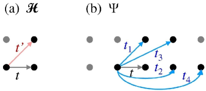
Figure 1: (a) Hopping processes in Hamiltonian [Eqs. (1) and (2)] and (b) those corresponding to band-adjusting parameters $t_{\eta}$ ($\eta=1$–$4$) in trial wave functions [Eqs. (13)-(17)]. In both figure, $t$ is the unit.

With cuprate SCs in mind, we consider the Hubbard model ($U\geq 0$) on a square lattice with diagonal hopping:

$${\cal H} = {\cal H}_{\rm kin}+{\cal H}_{U}$$ (1)

$$= -\sum_{(i,j),\sigma}t_{ij}\left(c^{\dagger}_{i\sigma}c_{j\sigma}+\mbox{H.c.}\right)+U\sum_{j}n_{j\uparrow}n_{j\downarrow},$$

where $c_{j\sigma}$ annihilates an electron of spin $\sigma$ at site $j$, $n_{j\sigma}=c^{\dagger}_{j\sigma}c_{j\sigma}$, and $(i,j)$ indicates the sum of pairs on sites $i$ and $j$. In this work, the hopping integral $t_{ij}$ is $t$ for nearest neighbors ($\geq 0$), $t^{\prime}$ for diagonal neighbors, and $0$ otherwise (${\cal H}_{\rm kin}={\cal H}_{t}+{\cal H}_{t^{\prime}}$) [Fig. 1(a)]. The bare energy dispersion becomes

$$\tilde{\varepsilon}_{\bf k}=-2t\left(\cos k_{x}+\cos k_{y}\right)-4t^{\prime}\cos k_{x}\cos k_{y}.$$ (2)

As we will see, the diagonal hopping term ${\cal H}_{t^{\prime}}$ plays a crucial role in the present theme. We use $t$ and the lattice spacing as the units of energy and length, respectively.

2.2 Trial wave functions

Because our interest here is to grasp the nature of BRE rather than obtain accurate numerical values, we employ forms of trial functions that capture the essence of physics but are as simple as possible. As many-body trial states, we use a Jastrow type, $\Psi={\cal P}\Phi$, where ${\cal P}$ is a two-body correlation factor (projector) and $\Phi$ is a one-body (mean-field-type) wave function. We use a simple form of ${\cal P}$ common to all trial states, ${\cal P}={\cal P}_{\rm G}{\cal P}_{Q}$, where ${\cal P}_{\rm G}$ is the well-known onsite Gutzwiller projector ${\cal P}_{\rm G}=\prod_{j}[1-(1-g)n_{j\uparrow}n_{j\downarrow}$][32] and ${\cal P}_{Q}$ is the nearest-neighbor doublon-holon (D-H) binding factor,[33, 34, 4]

$${\cal P}_{Q}=\prod_{j}\left[1-\zeta_{\rm d}d_{j}\prod_{\tau}\left(1-h_{j+\tau}\right)-\zeta_{\rm h}h_{j}\prod_{\tau}\left(1-d_{j+\tau}\right)\right],$$ (3)

where $d_{j}=n_{j\uparrow}n_{j\downarrow}$, $h_{j}=(1-n_{j\uparrow})(1-n_{j\downarrow})$, and $\tau$ runs over the nearest-neighbor sites of site $j$. As shown before,[36, 35] the D-H binding effect included in ${\cal P}_{Q}$ is crucial for properly treating Mott physics. The projector ${\cal P}$ has three variational parameters, $g$, $\zeta_{\rm d}$, and $\zeta_{\rm h}$, which trigger BR in $\Phi$.

Table 1: Elements modified by band renormalization in one-body part for finite systems (indicated by circles). The two elements merge for $L\rightarrow\infty$.

Modified elements	$\Phi_{\rm N}$	$\Phi_{d}$	$\Phi_{\rm AF}$	$\Phi_{\rm mix}$
$\{{\bf k}\}_{\rm occ}$ or Fermi surface	$\bigcirc$	$-$	$\bigcirc$	$\bigcirc$
Direct modification of $\varepsilon_{\bf k}$	$-$	$\bigcirc$	$\bigcirc$	$\bigcirc$

We turn to the one-body part $\Phi$, which is the main point for BRE. We start with the normal (paramagnetic) state. Let $\{{\bf k}\}_{\rm occ}$ denote the set of k points occupied by electrons in $\Phi$ according to $\varepsilon_{\bf k}\leq\varepsilon_{{\bf k}_{\rm F}}$ (or symbolically ${\bf k}\in{\bf k}_{\rm F}$). Then, the one-body normal state we use (a Fermi sea) is written as

$$\Phi_{\rm N}=\prod_{\{\bf k\}_{\rm occ},~{}\sigma}c^{\dagger}_{{\bf k},\sigma}|0\rangle.$$ (4)

If $\{{\bf k}\}_{\rm occ}$ is determined according to the bare band dispersion $\tilde{\varepsilon}_{\bf k}$ in Eq. (2), $\Phi_{\rm N}$ is the exact ground state of ${\cal H}$ for $U=0$. When the interaction is introduced, $\varepsilon_{\bf k}$ will be modified by its self-energy. In the framework of many-body variation theory, $\varepsilon_{\bf k}$ should be optimized along with the other parameters so as to reduce the total energy $E=\langle{\cal H}\rangle/N_{\rm s}$ ($N_{\rm s}$: number of sites). Note that in $\Phi_{\rm N}$ [Eq. (4)], $\varepsilon_{\bf k}$ does not explicitly appear but has the effect of determining $\{{\bf k}\}_{\rm occ}$ or the Fermi surface (see Table 1 for comparison). Namely, the operation of BR for $\Phi_{\rm N}$ is simply reduced to the choice of $\{{\bf k}\}_{\rm occ}$. To obtain full BRE, we need to find the $\{{\bf k}\}_{\rm occ}$ that yields the lowest $E/t$ among all the $\{{\bf k}\}_{\rm occ}$, but the number of choices of $\{{\bf k}\}_{\rm occ}$ grows exponentially [roughly as ${}_{N_{\rm s}/4}C_{N/8}$ ($N$: number of electrons)] as the system size grows. In this work, we optimize $E/t$ within the $\{{\bf k}\}_{\rm occ}$ that are generated by a tight-binding form of $\varepsilon_{\bf k}$ with diagonal transfer:

$$\varepsilon_{\bf k}^{\rm N}=-2t\left(\cos k_{x}+\cos k_{y}\right)-4t_{1}\cos k_{x}\cos k_{y},$$ (5)

where $t_{1}$ is varied. This form of $\varepsilon_{\bf k}$ has often been used for $d$-SC states in previous studies[21, 22, 23, 24, 25] and also seems reasonable as a first setting for $\Phi_{\rm N}$. Details of optimizing $\Psi_{\rm N}={\cal P}\Phi_{\rm N}$ are described in AppendixA. The ordered states $\Phi_{d}$, $\Phi_{\rm AF}$, and $\Phi_{\rm mix}$ introduced below are reduced to $\Phi_{\rm N}$ in the limit of $\Delta_{\rm AF}$ and/or $\Delta_{d}\rightarrow 0$.

We move on to the mixed state of AF and $d$-SC orders of a fixed electron number, $\Phi_{\rm mix}$. This state is written as a $d$-wave BCS state composed of AF quasiparticles:[18]

$$\Phi_{\rm mix}=\left(\sum_{\bf k}\phi({\bf k})~{}a_{{\bf k}\uparrow}^{\dagger}a_{{\bf-k}\downarrow}^{\dagger}\right)^{\frac{N}{2}}|0\rangle,$$ (6)

with

$$\phi({\bf k})=\frac{\Delta_{\bf k}}{\varepsilon^{\rm SC}_{\bf k}-\mu+\sqrt{(\varepsilon^{\rm SC}_{\bf k}-\mu)^{2}+\Delta_{\bf k}^{2}}}.$$ (7)

Here, $\mu$ is a variational parameter, which is reduced to the chemical potential for $U/t\rightarrow 0$, and a $d_{x^{2}-y^{2}}$-wave gap is assumed as

$$\Delta_{\bf k}=\Delta_{d}(\cos k_{x}-\cos k_{y}),$$ (8)

with $\Delta_{d}$ being a $d$-wave pairing gap parameter. As the AF quasiparticles in Eq. (6), we employ a form of an AF Hartree-Fock solution at half filling with $t^{\prime}/t=0$:

$$a^{\dagger}_{{\bf k},\sigma}=\alpha_{\bf k}c^{\dagger}_{{\bf k},\sigma}+\mbox{sgn}(\sigma)\ \beta_{\bf k}c^{\dagger}_{{\bf k}+{\bf Q},\sigma},$$ (9)

$$a^{\dagger}_{{\bf k}+{\bf Q},\sigma}=-\mbox{sgn}(\sigma)\ \beta_{\bf k}c^{\dagger}_{{\bf k},\sigma}+\alpha_{\bf k}c^{\dagger}_{{\bf k}+{\bf Q},\sigma},$$ (10)

where ${\bf Q}$ is the AF nesting vector $(\pi,\pi)$, $\mbox{sgn}(\sigma)=1$ ($-1$) for $\sigma=\uparrow$ ($\downarrow$), and

$$\alpha_{\bf k}\ (\beta_{\bf k})=\frac{1}{\sqrt{2}}\sqrt{1-(+)\frac{\varepsilon^{\rm AF}_{\bf k}}{\left(\varepsilon^{\rm AF}_{\bf k}\right)^{2}+\Delta_{\bf AF}^{2}}}.$$ (11)

Here, $\Delta_{\rm AF}$ corresponds to the AF gap parameter in the sense of mean-field theory.

To introduce BRE into $\Phi_{\rm mix}$, we extend the band dispersions $\varepsilon^{\rm SC}_{\bf k}$ in Eq. (7) and $\varepsilon^{\rm AF}_{\bf k}$ in Eq. (11) independently by including tight-binding hopping terms up to three-step processes shown in Fig. 1(b),

$$\varepsilon^{\Lambda}_{\bf k}=\gamma_{\bf k}+\varepsilon^{\Lambda}_{1}({\bf k})+\varepsilon^{\Lambda}_{2}({\bf k})+\varepsilon^{\Lambda}_{3}({\bf k})+\varepsilon^{\Lambda}_{4}({\bf k}).$$ (12)

with $\Lambda=$ SC or AF and

$$\gamma_{\bf k}=-2t(\cos k_{x}+\cos k_{y}),$$ (13)

$$\varepsilon^{\Lambda}_{1}({\bf k})=-4t^{\Lambda}_{1}\cos k_{x}\cos k_{y},$$ (14)

$$\varepsilon^{\Lambda}_{2}({\bf k})=-2t^{\Lambda}_{2}(\cos 2k_{x}+\cos 2k_{y}),$$ (15)

$$\varepsilon^{\Lambda}_{3}({\bf k})=-4t^{\Lambda}_{3}(\cos 2k_{x}\cos k_{y}+\cos k_{x}\cos 2k_{y}),\quad\qquad$$ (16)

$$\varepsilon^{\Lambda}_{4}({\bf k})=-2t^{\Lambda}_{4}(\cos 3k_{x}+\cos 3k_{y}).$$ (17)

Here, the eight band-adjusting parameters $t^{\Lambda}_{\eta}/t$ ($\Lambda=\mbox{SC}$ or AF, $\eta=1$–4) are independent of $t^{\prime}/t$ in ${\cal H}$ and are optimized along with the other variational parameters ($g$, $\zeta_{\rm d}$, $\zeta_{\rm h}$, $\Delta_{d}$, $\mu$, $\Delta_{\rm AF}$). Note that the ${\bf k}$ points used in Eqs. (9) and (10) belong to $\{{\bf k}\}_{\rm occ}$ determined by $\varepsilon^{\rm AF}_{\bf k}$ (not $\gamma_{\bf k}$).[37] As a result, if $\{{\bf k}\}_{\rm occ}$ includes ${\bf k}$ points outside the folded AF Brillouin zone, $\phi({\bf k})$ for the corresponding ${\bf k}$ in the sum in Eq. (6) is doubled, and $\phi({\bf k})$ for ${\bf k}$ ($\notin{\bf k}_{\rm F}$) inside the AF Brillouin zone becomes null. In $\Phi_{\rm mix}$, $\varepsilon^{\rm SC}_{\bf k}$ and $\varepsilon^{\rm AF}_{\bf k}$ are explicitly renormalized, and the weight of $\phi({\bf k})$ is also modified by $\{{\bf k}\}_{\rm occ}$ determined by $\varepsilon^{\rm AF}_{\bf k}$, as summarized in Table 1.

A pure one-body AF state $\Phi_{\rm AF}$ is given by the $\Delta_{d}\rightarrow 0$ limit of $\Phi_{\rm mix}$ as

$$\Phi_{\rm AF}=\prod_{\{{\bf k}\}_{\rm occ},~{}\sigma}a^{\dagger}_{{\bf k},\sigma}|0\rangle,$$ (18)

where the AF quasiparticles are given by Eqs. (9) and (10) and $\{{\bf k}\}_{\rm occ}$ is determined by $\varepsilon^{\rm AF}_{\bf k}$ in Eq. (12). There are five variational parameters ($t^{\rm AF}_{\eta}$, $\Delta_{\rm AF}$) in $\Phi_{\rm AF}$. A pure $d_{x^{2}-y^{2}}$-wave singlet pairing (BCS) state of a fixed electron number[38] is given by the $\Delta_{\rm AF}\rightarrow 0$ limit of $\Phi_{\rm mix}$ as

$$\Phi_{d}=\left(\sum_{\bf k}\phi({\bf k})~{}c_{{\bf k}\uparrow}^{\dagger}c_{{\bf-k}\downarrow}^{\dagger}\right)^{\frac{N}{2}}|0\rangle,$$ (19)

with $\phi({\bf k})$ given by Eq. (7). There are six variational parameters ($t^{\rm SC}_{\eta}$, $\Delta_{d}$, $\mu$) in $\Phi_{d}$.

2.3 Variational Monte Carlo calculations

In general, it is impossible to accurately calculate variational expectation values of a many-body wave function $\langle{\cal O}\rangle$, with ${\cal O}$ being an operator, by analytical means. Instead, in many cases, the expectation values can be accurately numerically estimated using VMC methods[39, 40, 41, 42]. Recently, many parameters (up to more than $10^{6}$) in $\langle{\cal H}\rangle$ have been efficiently optimized by newly introduced algorithms.[43] In the present cases, however, we cannot adopt ordinary optimization schemes using derivatives of energy because $E(\{\gamma\})$ is constant ($\Psi_{\rm N}$) or nearly constant ($\Psi_{\rm AF}$ and $\Psi_{\rm mix}$) as a function of the band parameters ($t_{\eta}^{\Lambda}$) in the parameter set $\{\gamma\}$ and has irregularly distributed discontinuities. To address BR in $\Psi_{\rm N}$, we combine a VMC method with the extrapolation scheme described in AppendixA. For $\Psi_{\rm AF}$ and $\Psi_{\rm mix}$, we repeat a primitive linear optimization method in this study until optimization becomes successful, although better ways are applicable. Details are described in AppendixB. For $\Psi_{d}$, ordinary optimization algorithms are applicable unless $\Delta_{d}$ approaches zero. For $\Delta_{d}\sim 0$, a difficulty similar to that for $\Psi_{\rm AF}$ manifests itself.

We calculate physical quantities using more than $2.5\times 10^{5}$ samples. The accuracy of the total energy of $10^{-4}t$ is preserved, similarly to in previous studies. It is laborious to accurately converge $\Delta_{\rm AF}$ (or $\Delta_{d}$) and the band parameters to specific values because there is redundancy among these parameters. However, this affects the calculations of physical quantities only slightly in most cases.

We use systems of $N_{\rm s}=L\times L$ sites with $L=10$–$18$ under periodic-antiperiodic boundary conditions. The closed-shell condition is not satisfied because we allow $\{{\bf k}\}_{\rm occ}$ to be optimized automatically, although the total momentum is preserved at zero. In this paper, we often consider rough system-size dependence for $\delta\sim 0.08$ using $L=10$, 12, 14, 16, and 18 with $N=92$, 132, 180, 236, and 296 ($\delta=0.08$, 0.0833, 0.0816, 0.0781, and 0.0864), respectively.

3 BRE on Pure $d$-Wave Pairing State

In this section, we discuss BRE on the pure $d$-wave pairing state without an AF order, $\Psi_{d}={\cal P}\Phi_{d}$. In Sect. 3.1, we confirm that there is a large BRE in $\Psi_{d}$, as found in previous studies.[21, 22, 23, 24, 25] In Sect. 3.2, however, we show that the improvement in energy is unexpectedly small. In Sect. 3.3, we also find that the modification of relevant physical quantities is negligible.

3.1 Large BRE for (doped) Mott insulators

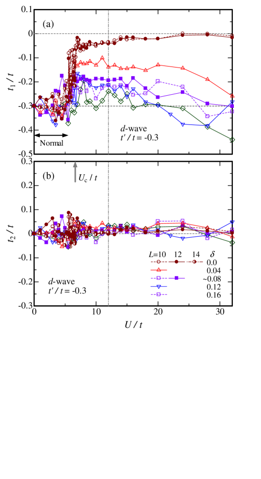
Figure 2: (Color online) Optimized band parameters (a) $t_{1}$ and (b) $t_{2}$ of $d$-wave singlet pairing state (BR2) as functions of $U/t$ for several doping rates. In (a), the area where $\Psi_{d}$ is reduced to $\Psi_{\rm N}$ is shown by an arrow labeled ‘Normal’. In (b), the Mott transition point at half filling is indicated by a gray arrow.

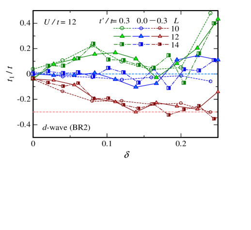
Figure 3: (Color online) Optimized values of $t_{1}/t$ for the $d$-wave pairing state (BR2) plotted as functions of doping rate for three values of $t^{\prime}/t$ in the regime of a doped Mott insulator ($U/t=12$).

First, we attempted to optimize $\Psi_{d}$ only with two band parameters $t_{1}$ and $t_{2}$ by putting $t_{3}=t_{4}=0$ for simplicity. We abbreviate this two-band-parameter optimization to BR2.

In Fig. 2(a), we show the optimized values of $t_{1}/t$ as functions of $U/t$, fixing the model parameter at $t^{\prime}/t=-0.3$. For $U/t\lesssim 5$, $t_{1}$ preserves the bare value $t_{1}\sim t^{\prime}$ irrespective of $\delta$; no substantial BR exists. This is because $\Delta_{d}$ is very small in this range of $U/t$ and the state is reduced to the normal state, as in the cases without BRE.[36, 4] $\Psi_{\rm N}$ also shows no substantial BR in this range of $U/t$ as shown in Sect. 4. The relatively large statistical fluctuation in the case of $\Delta_{d}\sim 0$ stems from the same difficulty as in $\Psi_{\rm N}$ in optimizing the band parameters [see AppendixA]. On the other hand, at $U=U_{\rm c}\sim 6.5t$[36] ($U_{\rm c}/t$: Mott transition point in $\Psi_{d}$), $t_{1}/t$ abruptly increases, in particular, $t_{1}/t$ approaches 0 at $\delta=0$. As previously pointed out,[21, 4] this BR of $\Psi_{d}$ occurs so that the quasi-Fermi surface overlaps with or approaches antinodal points [$(\pi,0)$, etc.], where the van Hove singularity exists for $|t^{\prime}/t|\leq 0.5$ and the $d$-wave gap becomes maximum. Furthermore, the elastic electron scattering of ${\bf q}={\bf Q}$ connects these points with opposite signs of $\Delta_{d}$. Restoration of the nesting condition, which is the principal cause of BRE for the AF state, seems a subordinate aspect for $\Psi_{d}$. As $\delta$ increases, $t_{1}$ slowly approaches the value of $t^{\prime}$ for the same reason (see Fig. 3). In contrast to $t_{1}/t$, the optimized $t_{2}/t$ remains almost zero (the bare value) for all $U/t$ and $\delta$ for $t^{\prime}/t=-0.3$, as shown in Fig. 2(b).

Table 2: Rough estimate of coefficients in fitting function Eq. (20) for $U/t=12$ estimated from data for $L=10$-$14$.

$\delta$	$0.0$	$0.04$	$\sim 0.08$	$0.12$	$0.16$
$\alpha_{+}$	$0.14$	$0.41$	$0.55$	$0.25$	$0.05$
$\alpha_{-}$	$0.14$	$0.41$	$0.67$	$0.90$	$0.95$

Next, we look at the $t^{\prime}/t$ dependence of $t_{1}/t$ and $t_{2}/t$ for $U>U_{\rm c}$. We find that the optimized $t_{1}/t$ is roughly fitted by separate linear functions of $t^{\prime}/t$ for the hole- and electron-doped cases:

$$t_{1}/t=\alpha_{\pm}(\delta)\times t^{\prime}/t,$$ (20)

where $\alpha_{+}(\delta)$ [$\alpha_{-}(\delta)$] is the coefficient for $t^{\prime}/t>0$ [$t^{\prime}/t<0$] at a fixed $\delta$. If $t_{\eta}$ ($\eta\geq 2$) is ineffective (we actually see it shortly), BRE are nonexistent for $\alpha_{\pm}=1$ and, inversely, $\varepsilon_{\bf k}^{\rm SC}$ is renormalized to the case of $t^{\prime}=0$ for $\alpha_{\pm}=0$. The values of $\alpha_{\pm}$ depend on $U/t$ only slightly and are shown for $U/t=12$ in Table 2. Although the magnitudes of BR exhibit opposite tendencies between $\alpha_{+}$ and $\alpha_{-}$ for $\delta\gtrsim 0.08$, $\alpha_{\pm}$ is always positive. As a result of this positiveness, the convexity ($t^{\prime}/t>0$) or concavity ($t^{\prime}/t<0$) of the bare Fermi surface near $(\pi/2,\pi/2)$ is preserved in the renormalized quasi-Fermi surface of $\varepsilon_{\rm k}^{\rm SC}$. As a result, the locus of a hot spot —the intersection of a (quasi-) Fermi surface and the AF Brillouin zone boundary, where scattering of ${\bf q}=(\pi,\pi)$ takes place—[44] is near $(\pi,0)$ for $t^{\prime}/t<0$ but approaches $(\pi/2,\pi/2)$ to some extent for $t^{\prime}/t>0$.[45, 24, 46] As we will see in Sect. 6.2, the loci of hot spots become a condition that a coexistent state arises.

In contrast to $t_{1}/t$, $t_{2}/t$ is again found to be almost zero for any $t^{\prime}/t$ and $\delta$. The effect of $t_{3}$ and $t_{4}$ is considered using $\Psi_{d}$ with four band parameters $t_{1}$–$t_{4}$ in $\varepsilon_{\bf k}$ [Eq. (12)] (BR4). The behavior of $t_{1}/t$ and $t_{2}/t$ for BR4 is basically similar to that for BR2 mentioned above. We found that both the optimized $t_{3}$ and $t_{4}$ have small positive values ($t_{3}/t\lesssim 0.11$, $t_{4}/t\lesssim 0.095$, at largest at half filling) almost independent of $t^{\prime}/t$. These values decrease as $\delta$ increases and almost vanish for $\delta\gtrsim 0.1$. As we will see in Sect. 3.2, the effects of $t_{3}$ and $t_{4}$ on energy and other quantities are also slight.

To summarize, BRE on $\Psi_{d}$ are large for $U\gtrsim U_{\rm c}$, $\delta\sim 0$ and large $|t^{\prime}/t|$. If these conditions are satisfied, the effective band tends to the bare band of a square lattice ($\varepsilon_{\bf k}\rightarrow\gamma_{\bf k}$ or $|t_{1}/t|\rightarrow 0$). This feature of BRE on the $d$-wave pairing state has already been pointed out in previous studies.[21, 22, 26, 27, 23, 24, 25]

3.2 Slight improvement in energy by BRE

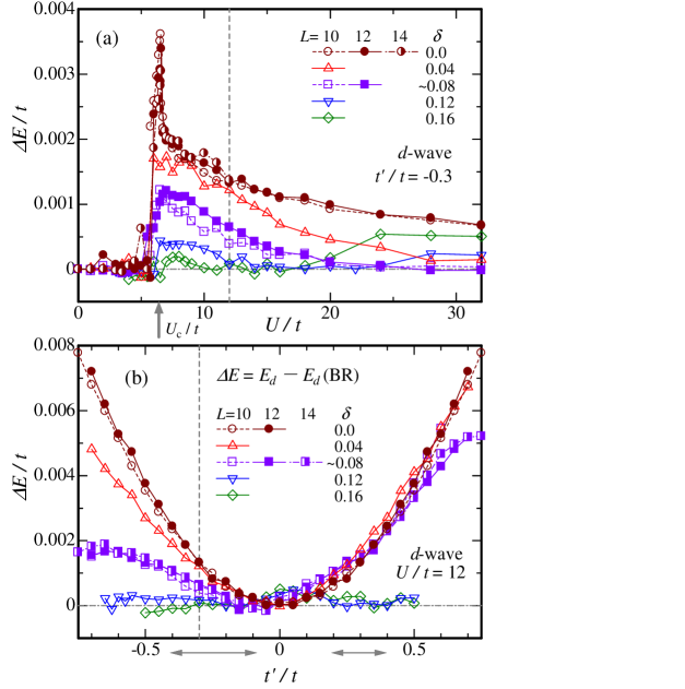
Figure 4: (Color online) Energy improvement [Eq. (21)] owing to BRE for the $d$-wave pairing state (BR2) shown for some values of $\delta$ and $L$, (a) as functions of correlation strength with $t^{\prime}/t=-0.3$ and (b) as functions of $t^{\prime}/t$ with $U/t=12$. The Mott transition point at half filling is indicated by a thick gray arrow in (a). In (b), plausible areas of $t^{\prime}/t$ for hole-doped ($t^{\prime}/t<0$) and electron-doped ($t^{\prime}/t>0$) cuprates are indicated with gray arrows.

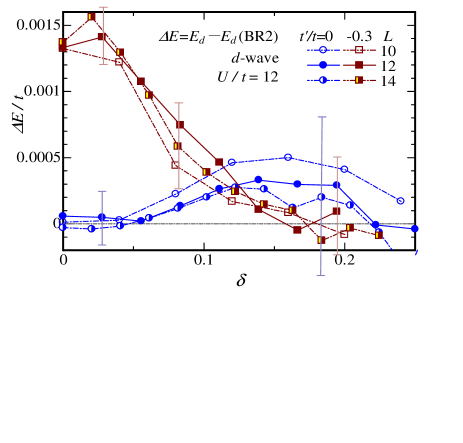
Figure 5: (Color online) Energy improvement [Eq. (21)] owing to BRE for the $d$-wave pairing state (BR2) plotted as functions of doping rate for two values of $t^{\prime}/t$ in a strongly correlated regime ($U/t=12$). Broad statistical errors are indicated by bars for some data points.

Here and in some later sections, we consider the improvement in the total energy per site owing to BRE, represented as

$$\Delta E=E_{\Lambda}-E_{\Lambda}(\mbox{BR}),\qquad(\Lambda=d,\mbox{N, or AF})$$ (21)

where $E_{d}$ [$E_{d}(\mbox{BR})$] is the energy of $\Psi_{d}$ without [with] BRE; $\Delta E/t\geq 0$ holds except for statistical errors. In Fig. 4(a), the $U/t$ dependence of $\Delta E/t$ is shown for some values of $\delta$ for $t^{\prime}/t=-0.3$. The regime of finite $\Delta E/t$ for $U>U_{\rm c}$ corresponds to that of the finite BR of $t_{1}/t$ shown in Fig. 2(a). As $\delta$ increases, both the magnitude of BR and $\Delta E/t$ decrease and almost vanish in the overdoped regime ($\delta\gtrsim 0.15$). Figure 4(b) shows the $t^{\prime}/t$ dependence of $\Delta E/t$ for $U/t=12$, which mostly corresponds to the degree of BR of $t_{1}/t$ given by Eq. (20) with $\alpha_{\pm}$ in Table 2. The exception for $t^{\prime}/t>0$ and large $\delta$ is caused by the vanishing of hot spots, which BRE alone cannot control. Shown in Fig. 5 is the $\delta$ dependence of $\Delta E/t$, which again corresponds to the degree of BRE on $t_{1}/t$ shown in Fig. 3.

Table 3: Examples of total energy per site shown for a specific case ($t^{\prime}/t=-0.3$, $U/t=12$, $L=10$) for comparison among four states with different BR levels and three doping rates. The brackets denote errors in the last digits.

State	Condition	$E/t$
	of $\varepsilon_{\bf k}$	$\delta=0.0$	$0.04$	$0.08$
Normal	no BR	$-0.1855(2)$	$-0.3230(2)$	$-0.4259(2)$
	BR	$-0.2660(1)$	$-0.3360(2)$	$-0.4310(1)$
$d$-wave	no BR	$-0.3222(2)$	$-0.3816(4)$	$-0.4602(2)$
	BR2	$-0.3235(2)$	$-0.3827(1)$	$-0.4606(3)$
	BR4	$-0.3241(2)$	$-0.3828(4)$	$-0.4606(10)$
AF	no BR	$-0.1879(2)$	$-0.3288(2)$	$-0.4259(2)$
	BR4	$-0.35319(2)$	$-0.4201(3)$	$-0.4881(1)$
Mixed	BR 4+4	$-0.3559(2)$	$-0.4211(2)$	$-0.4915(2)$

Now we are aware that the energy is basically improved according to the degree of BRE on $t_{1}/t$ for every model parameter. Nevertheless, what we should notice here is that the magnitude of $\Delta E/t$ is unexpectedly small. The precision (statistical error) of the energy in the present VMC calculations for $\Psi_{d}$ is on the order of $10^{-4}t$ as shown by bars in Fig. 5, while the maximum value of $\Delta E/t$ is only $\sim 10^{-3}t$ (only slightly larger than the errors). In Table 3, $E/t$ for $\Psi_{d}$ is compared among the cases of without BR, BR2, and BR4 for typical model parameters. We also find that the difference between BR2 and BR4 is very small. What is more, the difference in $\Psi_{d}$ is an order (two orders) of magnitude smaller than that in $\Psi_{\rm N}$ ($\Psi_{\rm AF}$) for any $\delta$ presented. This difference is visually perceived in Fig. 11.

3.3 Small modification of quantities by BRE

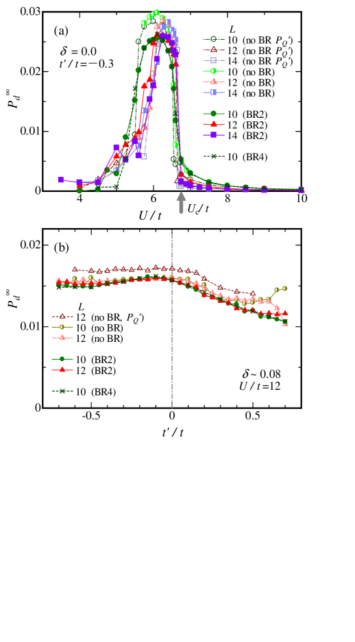
Figure 6: (Color online) Behavior of the $d$-wave SC correlation functions in $\Psi_{d}$ compared between BR cases and no-BR cases (a) at half filling and $t^{\prime}/t=-0.3$ as functions of $U/t$ and (b) for $\delta\sim 0.08$ and $U/t=12$ as a function of $t^{\prime}/t$. On the horizontal axis in (a), the Mott transition point is indicated by a thick gray arrow. The data for “no BR ${\cal P}_{Q}^{\prime}$” are adopted from Ref. Y2013, in which a similar but somewhat different D-H factor is used.

First, we consider a $d$-wave pairing correlation function,

$$P_{d}({\bf r})=\frac{1}{N_{\rm s}}\sum_{i}\sum_{\tau,\tau^{\prime}=\hat{\bf x},\hat{\bf y}}(-1)^{1-\delta(\tau,\tau^{\prime})}\left\langle{\Delta_{\tau}^{\dagger}({\bf R}_{i})\Delta_{\tau^{\prime}}({\bf R}_{i}+{\bf r})}\right\rangle,$$ (22)

where $\hat{\bf x}$ ($\hat{\bf y}$) denotes the lattice vector in the $x$ ($y$) direction, $\delta(\tau,\tau^{\prime})$ indicates the Kronecker delta, and $\Delta_{\tau}^{\dagger}({\bf R}_{i})$ is the creation operator of a nearest-neighbor singlet pair at site ${\bf R}_{i}$,

$$\Delta_{\tau}^{\dagger}({\bf R}_{i})=(c_{{i}\uparrow}^{\dagger}c_{{i}+\tau\downarrow}^{\dagger}+c_{{i}+\tau\uparrow}^{\dagger}c_{{i}\downarrow}^{\dagger})/{\sqrt{2}}.$$ (23)

If $P_{d}({\bf r})$ remains finite for $|{\bf r}|\rightarrow\infty$ ($P_{d}^{\infty}$), a $d$-wave off-diagonal long-range order exists; $P_{d}^{\infty}$ roughly represents the square of the SC gap. For $\Psi_{d}$, we estimate $P_{d}^{\infty}$ in the same way as discussed in Appendix C in Ref. Y2013. As an example, in Fig. 6(a), we show $P_{d}^{\infty}$ at half filling for some levels of BR (and ${\cal P}$) for $L=10$-$14$. As discussed in Ref. Y2013, $P_{d}^{\infty}$ is negligible for small values of $U/t$. As $U/t$ increases, $P_{d}^{\infty}$ abruptly increases at $U/t\sim 5$, exhibits a sharp peak near the Mott transition point $U_{\rm c}/t\sim 6.5$, and vanishes in the Mott insulator regime $U>U_{\rm c}$. Although the peak value of $P_{d}^{\infty}$ tends to be slightly decreased by BRE, the behavior does not vary as a whole. For $\delta>0$, the area where $P_{d}^{\infty}$ is sizable extends to large values of $U/t$, but the modification of $P_{d}^{\infty}$ by BRE remains small (not shown). The modification of $P_{d}^{\infty}$ is also small when $t^{\prime}/t$ is varied, as shown in Fig. 6(b). Furthermore, the difference between BR2 and BR4 is negligible.

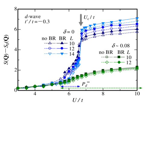
Figure 7: (Color online) Spin structure factor at ${\bf Q}=(\pi,\pi)$ measured from the bare ($U=0$) value $S_{0}({\bf Q})$ ($=1$) compared between BR2 and no-BR cases for $\delta=0$ and $\sim 0.08$ for $t^{\prime}/t=-0.3$ as functions of $U/t$. A few cases with different values of $L$ are shown. The Mott transition point at half filling are indicated by a thick gray arrow. Near the horizontal axis, the areas where the $d$-wave correlation function $P_{d}^{\infty}$ becomes sizable are indicated by dashed arrows for $\delta=0$ (blue) and $\sim 0.08$ (green). See Fig. 6 for $\delta=0$.

Next, we look at the ${\bf q}={\bf Q}$ element of the spin structure factor

$$S({\bf q})=\frac{1}{N_{\rm s}}\sum_{ij}{e^{i{\bf q}\cdot({\bf R}_{i}-{\bf R}_{j})}\left\langle{S_{i}^{z}S_{j}^{z}}\right\rangle}.$$ (24)

The $U/t$ dependence of $S({\bf Q})$ is shown in Fig. 7 for $\delta=0$ and $\sim 0.08$. As previous studies pointed out, an increase in $S({\bf Q})$ is necessary for an increase in $P_{d}^{\infty}$ because the electron scattering of ${\bf Q}$ yields an attractive force for pairing. Anyway, the modification of $S({\bf Q})$ by BRE is also small and only quantitative even at half filling.

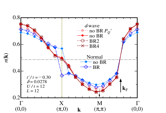
Figure 8: (Color online) Comparison of momentum distribution function of $d$-wave pairing state (red and brown) among various levels of BR (and ${\cal P}_{Q}$) in the regime of doped Mott insulators ($U/t=12$) along the path $(0,0)\rightarrow(\pi,0)\rightarrow(\pi,\pi)\rightarrow(0,0)$. The Fermi surface in the nodal ($\Gamma$-M) direction is indicated by an arrow labeled ${\bf k}_{\rm F}$. For comparison, we add $n({\bf k})$ for the normal state (blue) with and without BRE as discussed in Sect. 4.

Finally, we discuss the momentum distribution function

$$n({\bf k})=\frac{1}{2}\sum_{\sigma}\langle c^{\dagger}_{\bf k\sigma}c_{\bf k\sigma}\rangle.$$ (25)

It seems that $n({\bf k})$ sensitively reflects the variation of the effective band $\varepsilon_{\bf k}$, which is considerably renormalized depending on the case. Figure 8 depicts $n({\bf k})$ in such cases with red (without BRE) and brown (with BRE) symbols for $\Psi_{d}$ and blue symbols for the normal state $\Psi_{\rm N}$ (see Sect. 4). In accordance with the above expectation, the locus of ${\bf k}_{\rm F}$ (discontinuity) near the X point in $\Psi_{\rm N}$ is shifted to a neighbor ${\bf k}$ point by BRE. Nevertheless, in $\Psi_{d}$, the modification by BRE is very small for the gap behavior in the antinodal area (${\bf k}\sim$X) as well as for the discontinuity in the nodal direction [${\bf k}\sim(\pi/2,\pi/2)$], despite the large BRE ($t_{1}/t\sim-0.05$ for $t^{\prime}/t=-0.3$ in Fig. 3). This is probably because the choice of $\{\bf k\}_{\rm occ}$, which is controlled by $\varepsilon_{\bf k}$ in $\Psi_{\rm N}$ and $\Psi_{\rm AF}$, is unnecessary in $\Psi_{d}$ as shown in Table 1.

In summary, the BR of $\varepsilon_{\bf k}^{\rm SC}$ itself is large ($t_{1}/t\rightarrow 0$) for $U\gtrsim U_{\rm c}$, large $|t^{\prime}/t|$, and $\delta\sim 0$, as previous studies elucidated. Notwithstanding, BRE on relevant quantities as well as on the energy for $\Psi_{d}$ are very small and insignificant compared with those on the normal and AF states discussed below.

4 BRE on Normal (Paramagnetic) State

In this section, we discuss BRE on the normal or paramagnetic state (projected Fermi sea),

$$\Psi_{\rm N}={\cal P}\Phi_{\rm N}={\cal P}\prod_{\{{\bf k}_{\rm occ}\},\sigma}c^{\dagger}_{{\bf k},\sigma}|0\rangle.$$ (26)

We cannot apply ordinary optimization procedures to $\Psi_{\rm N}$ that use the gradients of $E/t$ with respect to band parameters because $E/t$ for $\Psi_{\rm N}$ with a finite $N$ is constant in a certain area of the band-parameter space. Hence, we must resort to a different way of optimizing $\Psi_{\rm N}$, which is described in AppendixA. Here, we focus on the features of the optimized $\Psi_{\rm N}$.

Before discussing BRE, we briefly review some aspects of $\Psi_{\rm N}$ without BRE ($t_{1}=t^{\prime}$).[36, 4] At half filling, a Mott transition occurs at $U_{\rm c}/t\sim 8.5$ for $t^{\prime}/t=0$; $U_{\rm c}/t$ increases as $|t^{\prime}/t|$ increases: $U_{\rm c}/t\sim 11.2$ for $|t^{\prime}/t|=0.3$. Although the Mott transition does not exist for $\delta>0$, the nature of $\Psi_{\rm N}$ markedly changes at $U\sim U_{\rm c}$. For $U\gtrsim U_{\rm c}$, $\Psi_{\rm N}$ is not a simple metal but takes on a typical feature of Mott physics (D-H binding effect) as a doped Mott insulator.

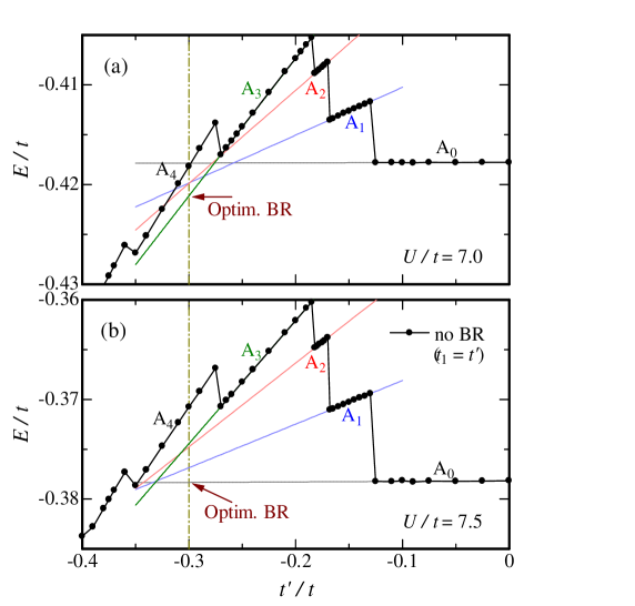
Figure 9: (Color online) Total energy of $\Psi_{\rm N}$ at half filling compared between the cases of (a) $U/t=7.0$ and (b) $7.5$ as a function of $t^{\prime}/t$. Solid circles indicate $E/t$ without BRE, namely $t_{1}=t^{\prime}$. A_ℓ ($\ell$: integer) indicates the area of $t^{\prime}/t$ corresponding to $\{{\bf k}_{\ell}\}_{\rm occ}$. The optimized energy owing to BRE is given by the lowest value among all extrapolated lines. For $t^{\prime}/t=-0.3$, the optimized value of $E/t$ is indicated by an arrow in each panel. A detailed explanation of the optimization is given in AppendixA.

Now, we consider BRE. Because BRE are inefficient or weak for $t^{\prime}/t\sim 0$, similarly to the case of $\Psi_{d}$, we first consider the moderate case $t^{\prime}/t=-0.3$. We start with half-filled cases. Similarly to in $\Psi_{d}$, the energy reduction by BRE is zero or very small for $U/t\lesssim 6$, even if the optimized $t_{1}$ (accurately, the area including $t_{1}$) somewhat shifts from $t^{\prime}$ (the area including $t^{\prime}$). As shown in Fig. 9 for $L=14$, the optimized energy indicated by an arrow is given by $\{{\bf k}_{3}\}_{\rm occ}$ (${\rm A}_{3}=[-0.27,-0.19]$) for $U/t=7.0$, while it is given by $\{{\bf k}_{0}\}_{\rm occ}$ (${\rm A}_{0}=[-0.125,0.125]$) for $U/t=7.5$. Namely, the optimized band parameter $t_{1}$ rapidly varies from $\sim t^{\prime}$ ($\in{\rm A}_{3}$) to $\sim 0$ ($\in{\rm A}_{0}$) between $U/t=7.0$ and $7.5$ in this case, and the nesting condition is restored. For $U/t\gtrsim 7$, the optimized $\{{\bf k}\}_{\rm occ}$ remains equal to $\{{\bf k}_{0}\}_{\rm occ}$, or the optimized value of $t_{1}/t$ remains $\sim 0$ ($\varepsilon^{\rm N}_{\bf k}=\gamma_{\bf k}$). Also the renormalized state becomes identical to the normal state without BR of the simple square lattice, whose behavior is reviewed above.[36] Owing to BRE, the Mott transition point for $t^{\prime}/t=-0.3$ shifts from $U_{\rm c}/t\sim 11.2$ to $\sim 8.5$. In fact, the optimal energy at $U/t=8.5$ for $|t^{\prime}/t|\lesssim 0.5$ ($L=12$) is given by $\{{\bf k}_{0}\}_{\rm occ}$; thus, if BRE are introduced, the properties of the Mott transitions and Mott insulators for $|t^{\prime}/t|\lesssim 0.5$ are reduced to those for the simple square-lattice case ($t^{\prime}=0$) without BRE.

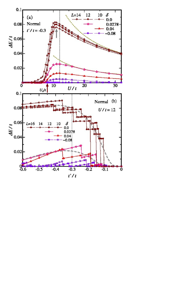
Figure 10: (Color online) Energy improvement [Eq. (21)] owing to BRE for the normal state shown for some doping rates and values of $L$, (a) as functions of correlation strength with $t^{\prime}/t=-0.3$, and (b) as a function of $t^{\prime}/t$ ($<0$) with $U/t=12$. In (a), the Mott transition points at half filling are indicated by thick arrows (brown for BR case, gray for no-BR case). Guide lines proportional to $t/U$ are added (dashed lines). In (b), data for each $\delta$ are well fitted by $\Delta E/t=-(\alpha/x)\exp(\beta/x)+\gamma x$ with $x=t^{\prime}/t$ and $\alpha$, $\beta$, and $\gamma$ being positive constants, as shown with gray dashed lines.

In Fig. 10(a), we show the energy reduction owing to BRE [Eq. (21)] for $t^{\prime}/t=-0.3$ as a function of $U/t$. At half filling, as $U/t$ increases, $\Delta E/t$ abruptly increases at $U/t\sim 7$ owing to the reason mentioned above, roughly as $\Delta E/t=\alpha\exp(-\beta t/U)$ with $\alpha$ and $\beta$ being positive constants. Then, $\Delta E/t$ exhibits a peak at $U/t\sim 11$, which corresponds to $U_{\rm c}/t$ for the case without BRE, then slowly decreases (proportionally to $t/U$ for $U/t\rightarrow\infty$). As the doping rate increases from $\delta=0$, the overall feature of the $U/t$ dependence is preserved but the magnitude rapidly decreases. For all the doping rates shown, $\Delta E/t$ is negligible for a weakly correlated regime ($U/t\lesssim 7$), meaning that appreciable BRE are also a characteristic of strong correlation for the normal state. In Fig. 10(b), the $t^{\prime}/t$ dependence ($t^{\prime}/t<0$) of $\Delta E/t$ is shown in the regime of Mott physics ($U/t=12$) for some doping rates. The BRE are largest at $|t^{\prime}/t|\sim 0.3$-$0.4$ and slight for $|t^{\prime}/t|\sim 0$.

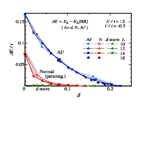
Figure 11: (Color online) Energy improvement [Eq. (21)] by BRE compared among the normal, AF (Sect. 5), and $d$-wave pairing (Sect. 3) states as functions of doping rate. Data for some system sizes are plotted. The thick pink dash-dotted line is a curve fitted using Eq. (27) with $\Psi_{\rm N}$ for all values of $L$.

We turn to the doping dependence of $\Delta E/t$. Shown in Fig. 11 is $\Delta E/t$ for $U/t=12$ and $t^{\prime}/t=-0.3$; these values are marked with vertical gray lines in Fig. 10. As $\delta$ increases, $\Delta E/t$ rapidly decreases as

$$\Delta E/t\propto\alpha\exp(-\delta/\delta_{\rm N}),$$ (27)

with $\delta_{\rm N}\sim 0.022$ ($\alpha$ : positive constant) in this case, as shown with a thick dash-dotted line in Fig. 11. Thus, BRE substantially vanishes for $\delta\gtrsim 0.1$. However, it should be emphasized that $\Delta E$ for $\Psi_{\rm N}$ is much larger than that for $\Psi_{d}$ near half filling, as shown in Fig. 11, and the BRE on $\Psi_{\rm N}$ are never negligible.

Finally, we analyze $\Delta E$ by dividing it into three components: $\Delta E=\Delta E_{t}+\Delta E_{t^{\prime}}+\Delta E_{U}$. We find that $\Delta E_{t}$ is positive and becomes large for a large $|t^{\prime}/t|$, while $\Delta E_{U}$ is negative and its magnitude is relatively small. Namely, the effective band is transformed so as to gain kinetic energy $E_{t}$ at the cost of the interaction energy $E_{U}$. This corresponds to a general tendency for a state in a strongly correlated regime to undergo a transition to reduce the kinetic energy.[35, 36] This feature applies to $\Psi_{\rm AF}$ and $\Psi_{\rm mix}$. For $\Delta E_{t^{\prime}}$, the magnitude is small as compared with those of the other two components, except for $t^{\prime}/t\sim-0.1$.

5 BRE on Pure Antiferromagnetic State

In this section, we consider the features of BRE on the AF state without a SC order,

$$\Psi_{\rm AF}={\cal P}\Phi_{\rm AF}.$$ (28)

In Sect. 5.1, we discuss the optimized parameters. In Sect. 5.2, a large improvement in energy due to BRE is revealed. In Sect. 5.3, topics associated with the Lifshitz transition are considered. Details of optimizing $\Psi_{\rm AF}$ are given in AppendixB.

5.1 Optimized band parameters

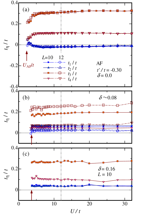
Figure 12: (Color online) Optimized band parameters in pure AF state for $t^{\prime}/t=-0.3$ plotted as functions of correlation strength. The doping rate is different among the three panels. The legends displayed in (a) are common to (b) and (c). The arrow in each panel indicates the AF transition point.

We start by clarifying the features of the optimized band parameters in $\Psi_{\rm AF}$, for which we always use $t_{\eta}$ ($\eta=1$–$4$) (BR4). In Fig. 12, the $U/t$ dependence of the optimized value of $t_{\eta}$ is shown for $t^{\prime}/t=-0.3$. For a small $U/t$ ($<U_{\rm AF}/t\sim 2.75$–$3.5$ for $t^{\prime}/t=-0.3$), no AF order exists and $\Psi_{\rm AF}$ is reduced to $\Psi_{\rm N}$. At $U=U_{\rm AF}$ (AF transition point), $\Delta_{\rm AF}$ and the sublattice magnetization (AF order parameter)

$$m=\frac{2}{N_{\rm s}}\sum_{j}\left|e^{i{\bf Q}\cdot{\bf r}_{j}}\langle S^{z}_{j}\rangle\right|$$ (29)

suddenly become finite (not shown), probably as a first-order transition, for $t^{\prime}/t\neq 0$. For $U>U_{\rm AF}$, marked BRE appears and $t_{\eta}$ becomes almost constant as a function of $U/t$. Although $t_{\eta}$ is almost invariant as a function of $U/t$, it varies with $\delta$ to some extent, at least for $t^{\prime}/t=-0.3$, as seen in Fig. 12. In fact, this feature depends on $t^{\prime}/t$, as described in the next paragraph. Anyway, we find that $\varepsilon_{\bf k}^{\rm AF}$ is renormalized so as to restore the nesting condition, irrespective of $\delta$.

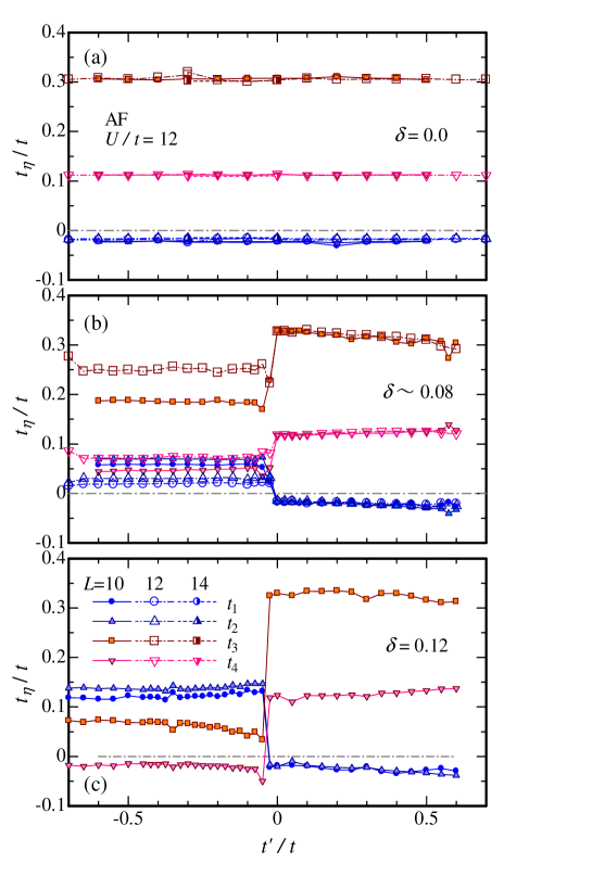
Figure 13: (Color online) Optimized band parameters in pure AF state for $U/t=12$ plotted as functions of $t^{\prime}/t$. The doping rate is different among the three panels. In (a), (b), and (c), data for $L=10$–$14$, $10$ and $12$, and $10$ are plotted respectively. The legends displayed in (c) are common to (a) and (b). The arrows in (b) and (c) indicate the values of $t^{\prime}_{\rm L}/t$.

Shown in Fig. 13 is the $t^{\prime}/t$ dependence of the optimized $t_{\eta}/t$ for $U/t=12$. At half filling [(a)], the renormalized values of $t_{\eta}/t$ and the other variational parameters (not shown) are constant with respect to $t^{\prime}/t$. The optimized AF state is independent of $t^{\prime}/t$; this feature is common to all values of $U/t$ ($>U_{\rm AF}/t$). In contrast, for $\delta>0$ [(b) and (c)], $t_{\eta}/t$ discontinuously changes at $t^{\prime}=t^{\prime}_{\rm L}\sim-0.05t$, and the other parameters (not shown) also exhibit singular behaviors (a cusp or discontinuity) there. Checking various cases, we find that the value of $t^{\prime}_{\rm L}/t$ subtly varies as the model parameters ($\delta$, $L$) vary but is necessarily situated in the range $-0.1<t^{\prime}_{\rm L}/t<0$. Thus, in doped cases, the AF phase is divided into two subphases according to whether $t^{\prime}>t^{\prime}_{\rm L}$ [type (i)] or $t^{\prime}<t^{\prime}_{\rm L}$ [type (ii)]. In each subphase, the $t^{\prime}/t$ dependence of $t^{\prime}_{\eta}/t$ is weak. However, the $\delta$ dependence of $t_{\eta}$ is weak in the type-(i) AF, whereas $t^{\prime}_{\eta}$ changes markedly as $\delta$ increases in the type-(ii) AF. Thus, the effective band $\varepsilon_{\bf k}^{\rm AF}$ will be distinct between the two subphases. As we will discuss in Sects. 5.3 and 6, this transition is regarded as a Lifshitz transition in the AF phase.

Finally, let us compare the optimized $\varepsilon_{\bf k}^{\rm SC}$ and $\varepsilon_{\bf k}^{\rm AF}$. $t_{1}/t$, which is the sole effective band parameter in $d$-SC, behaves as a linear function of $t^{\prime}/t$ with a positive coefficient [Eq. (20) and Table 2], indicating that BRE are mild, and a trace of the bare band remains [see Fig. 31(a) later]. On the other hand, for the AF part, BRE are prominent in that $t_{\eta}/t$ is almost independent of $t^{\prime}/t$, and for $t^{\prime}<t^{\prime}_{\rm L}$, the sign of $t_{1}/t$ becomes opposite that of $t^{\prime}/t$ [Figs. 13(b) and 13(c)]. Generally, the optimized forms of $\varepsilon_{\bf k}^{\rm SC}$ and $\varepsilon_{\bf k}^{\rm AF}$ are distinct, particularly, in the case of $t^{\prime}<t^{\prime}_{\rm L}$. This applies to the mixed state.

5.2 Large energy reduction by BRE

As shown in a previous VMC study without BRE,[4] the energy of the AF state is not lowered with respect to the paramagnetic state even at half filling for $|t^{\prime}/t|>0.35$–$0.41$ (depending on $L$) and $U/t=12$ (see Fig. 15 later). For $\delta>0$ and $t^{\prime}/t<0$, this boundary value of $|t^{\prime}/t|$ tends to decrease; for example, for $t^{\prime}/t=-0.3$, the optimized AF gap $\Delta_{\rm AF}$ substantially vanishes for $\delta\gtrsim 0.03$. However, as discussed in preceding reports,[29, 30] the AF state $\Psi_{\rm AF}$ with BRE [Eq. (28)] is stabilized with respect to $\Psi_{\rm N}$ up to $\delta\sim 0.16$ ($0.21$) for $t^{\prime}/t=0$ ($\pm 0.3$). First, we look at this great improvement by BRE more systematically.

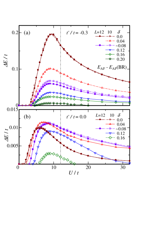
Figure 14: (Color online) Energy gain brought about by BRE in $\Psi_{\rm AF}$ plotted as a function of $U/t$ for (a) $t^{\prime}/t=-0.3$ and (b) $t^{\prime}/t=0$. Note that the scale on the vertical axis in (a) is 10 times larger than that in (b). Data for several doping rates are shown.

In Fig. 14, we show the $U/t$ dependence of the energy reduction by BRE [Eq. (21)]. In contrast to the case of $d$-wave pairing, a very large energy improvement is brought about by BRE for $U>U_{\rm AF}$, consistent with the large BR shown in Fig. 12 for $t^{\prime}/t=-0.3$. Energy improvement occurs even for $t^{\prime}/t=0$ [Fig. 14(b)] because the BRE on $t_{3}$ and $t_{4}$ are not small, as seen in Fig. 13, although $\Delta E/t$ is an order of magnitude smaller than that for $t^{\prime}/t=-0.3$. The $U/t$ dependence of $\Delta E/t$ for $t^{\prime}/t=0.3$ (not shown) is quantitatively similar (somewhat smaller for a large $\delta$) to the case of $t^{\prime}/t=-0.3$. We find from Fig. 14(a) that $\Delta E/t$ is a monotonically decreasing function of $\delta$ for a large $|t^{\prime}/t|$ (actually, when $t^{\prime}/t\lesssim-0.2$ and $t^{\prime}/t\gtrsim 0.3$). This has been illustrated in Sect. 4, where the $\delta$ dependence of $\Delta E/t$ in $\Psi_{\rm AF}$ was shown in Fig. 11 for $U/t=12$ and $t^{\prime}/t=-0.3$. $\Delta E/t$ decreases as $\delta$ increases, but the area of finite $\Delta E/t$ is considerably extended up to $\delta\sim 0.22$ for this parameter set. We repeat that the energy reduction by BRE in $\Psi_{\rm AF}$ is much larger than that in the normal and $d$-wave states. Such an improvement occurs in wide ranges of $U/t$ ($>U_{\rm AF}/t$) and $t^{\prime}/t$ ($\lesssim-0.15$).

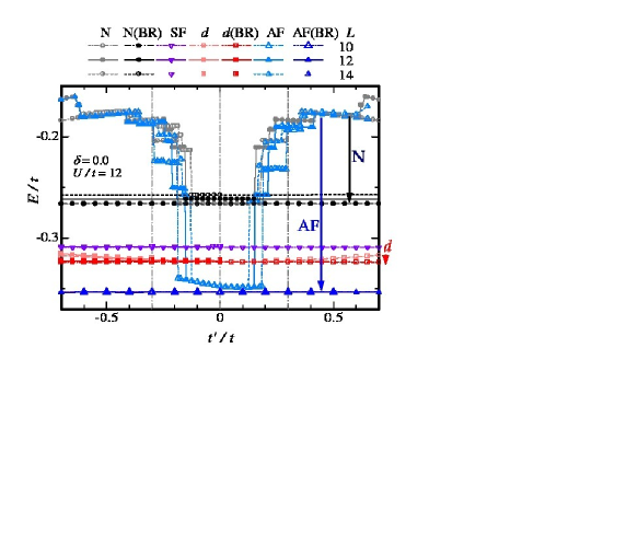
Figure 15: (Color online) Total energy at half filling for $U/t=12$ compared among various states with or without BR as a function of $t^{\prime}/t$. Dark (pale) symbols indicate cases with (without) BRE. Open, filled, and half-filled symbols indicate the data of $L=10$, $12$, and $14$, respectively. Arrows denote the energy reductions brought about by BRE for the different states. ‘SF’ indicates a staggered flux state.

Now, we compare the total energy among various states in the regime of Mott physics ($U>U_{\rm c}$). In Fig. 15, we compare the $t^{\prime}/t$ dependence of $E/t$ at half filling among $\Psi_{\rm N}$, $\Psi_{d}$, and $\Psi_{\rm AF}$. For each, the values with BRE and without BRE are plotted. Without BRE, the total energy more or less depends on $t^{\prime}/t$, whereas if BRE are introduced, $\Psi_{\Lambda}(t^{\prime}/t)$ ($\Lambda=$N, $d$, AF) is optimized at $\Psi_{\Lambda}(0)$ for any $t^{\prime}/t$. Consequently, $E/t$ becomes independent of $t^{\prime}/t$ because the diagonal hopping energy vanishes:

$$E_{t^{\prime}}\equiv\langle{\cal H}_{t^{\prime}}\rangle=0\qquad(\mbox{for }\delta=0),$$ (30)

and $E_{t}$ and $E_{U}$ become constant with respect to $t^{\prime}/t$. As a result, the energy of $\Psi_{\rm AF}$ (and $\Psi_{\rm N}$) is greatly reduced for large values of $|t^{\prime}/t|$. The order of the energy becomes

$$E_{\rm AF}<E_{d}<E_{\rm SF}<E_{\rm N}$$ (31)

for a wide range of $|t^{\prime}/t|$ (at least $<0.7$) at a fixed $U/t$ ($>U_{\rm c}/t$). Here, ‘SF’ indicates a staggered flux state, which is a candidate pseudogap state in cuprates[3, 47] and will be taken up in Sect. 6.3.

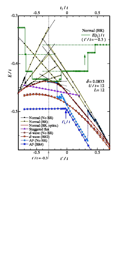
Figure 16: (Color online) Comparison of total energy among normal, AF, $d$-wave, and staggered flux[47] states with some levels of BR as a function of $t^{\prime}/t$ for $L=12$, $\delta=0.0833$, and $U/t=12$. The blue arrow indicates the Lifshitz transition point of the AF state. In addition, we give an illustration of the procedure for obtaining the optimized energy with BRE for the normal state (red line) from raw data without BRE (black circles) for $t^{\prime}/t=-0.3$. The green line denotes the variational energy for BRE as a function of $t_{1}/t$ (upper axis) for $t^{\prime}/t=-0.3$, which corresponds to the dark-green line in Fig. 37. For details, see AppendixA.

To consider doped cases ($\delta>0$), $E/t$ for various states are compared in Fig. 16 for $\delta=0.0833$ ($L=12$). Similar results for other values of $\delta$ were presented in Fig. 2 in a preceding report.[31] The energy reduction in $\Psi_{\rm AF}$ brought about by BRE for large $|t^{\prime}/t|$ is still sizable, and $E/t$ exhibits different linear behaviors on opposite sides of the Lifshitz transition point $t^{\prime}_{\rm L}/t$. In $\Psi_{\rm N}$ and $\Psi_{d}$, $E/t$ tends to decrease for $t^{\prime}/t>0$ as $t^{\prime}/t$ increases, and also decreases for $t^{\prime}/t\lesssim-0.4$–$-0.5$ as $|t^{\prime}/t|$ increases, mainly owing to the decrease in $E_{t^{\prime}}$. Consequently, the order in Eq. (31) does not change for a wide range of $\delta$ except for is the SF state, where it rapidly becomes unstable, especially for $t^{\prime}/t>0$.[47] Incidentally, by analyzing the charge-density structure factor, we find that $\Psi_{\rm AF}$ becomes metallic for $\delta<0$.[29] At any rate, $\Psi_{\rm AF}$ with BRE has much lower energy than $\Psi_{d}$ in the whole range of $t^{\prime}/t$ in Fig. 16. This is not the case for $\Psi_{\rm AF}$ without BRE (see also Table 4).

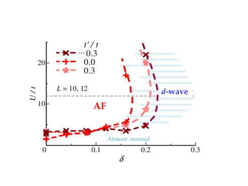
Figure 17: (Color online) Rough phase diagram in $U/t$-$\delta$ space constructed within $\Psi_{\rm AF}$ and $\Psi_{d}$, both with BRE. Because the dashed border lines indicate the locus of vanishing AF orders, the region of the $d$-wave may somewhat extend to the AF side. The region of the $d$-wave is schematic, especially, on the large-$\delta$ side.

By drawing similar figures for various values of $U/t$, $t^{\prime}/t$, and $\delta$, we construct the phase diagram in the $U/t$-$\delta$ space shown in Fig. 17. It is notable that, in contrast to previous studies, the AF area for $t^{\prime}/t=-0.3$ becomes wider than those for $t^{\prime}/t=0$ and $0.3$ and covers a very wide range of model parameters $U/t$, $t^{\prime}/t$, and $\delta$.

5.3 Lifshitz transition and electron-hole asymmetry

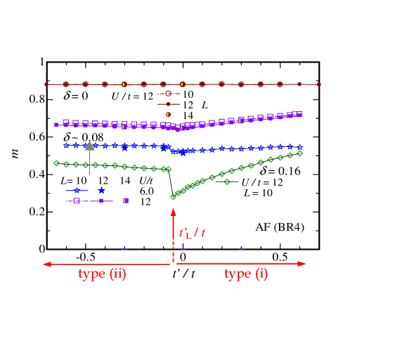
Figure 18: (Color online) Sublattice magnetization [Eq. (29)] in the AF phase plotted as a function of $t^{\prime}/t$ for some values of $\delta$ and $U/t$. The red arrow indicates the Lifshitz transition point.

Before discussing the Lifshitz transition, we mention the behavior of the staggered magnetization [Eq. (29)] in $\Psi_{\rm AF}$. We find that $m$ gradually increases as $U/t$ increases for $U_{\rm AF}<U\lesssim 12t$ and is almost constant for $U\gtrsim 12t$, irrespective of $\delta$ and $t^{\prime}/t$ (not shown). Shown in Fig. 18 is the $t^{\prime}/t$ dependence of $m$ for some values of $\delta$ and $U/t$. At half filling, $m$ is constant and $\sim 0.88$ ($m$ becomes 1 for the Néel state) because $\Psi_{\rm AF}$ is invariant for $t^{\prime}/t$, as mentioned in Sect. 5.1. For $\delta>0$, an anomaly appears at $t^{\prime}=t^{\prime}_{\rm L}$, and the difference in the two areas becomes more conspicuous as $\delta$ increases.

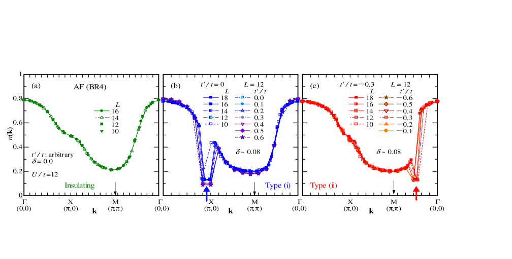
Figure 19: (Color online) Momentum distribution function plotted along the path $\Gamma\rightarrow{\rm X}\rightarrow{\rm M}\rightarrow\Gamma$ for $U/t=12$ in three cases: (a) half-filled case, in which $\Psi_{\rm AF}$ becomes independent of $t^{\prime}/t$, (b) doped case ($\delta\sim 0.08$) with $t^{\prime}>t^{\prime}_{\rm L}$ [type (i)], and (c) doped case ($\delta\sim 0.08$) with $t^{\prime}<t^{\prime}_{\rm L}$ [type (ii)]. Data for $L=10$-$18$ are plotted together. Pocket Fermi surfaces for the doped cases are indicated by thick arrows.

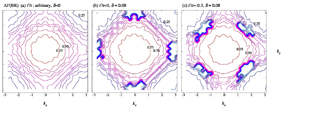
Figure 20: (Color online) Contour maps of momentum distribution function $n({\bf k})$ of the optimized pure AF state for $U/t=12$ shown for (a) $\delta=0$ with arbitrary $t^{\prime}/t$ and for $\delta\sim 0.08$ with (b) $t^{\prime}/t=0$ [type (i)] and (c) $-0.3$ [type (ii)]. The parameters in (a), (b), and (c) correspond to those in (a), (b), and (c) in Fig. 19, respectively. The maps are constructed using data for $L=10$–$18$. In these contour maps (and similar ones displayed henceforth), the fourfold rotational symmetry is somewhat smeared on account of anisotropic boundary conditions, open-shell conditions, and functions of the graphic software used.

To confirm that the transition arising at $t^{\prime}_{\rm L}/t$ is a kind of Lifshitz transition, we plot in Fig. 19 the momentum distribution function [Eq. (25)] in $\Psi_{\rm AF}$ for $U/t=12$ along the path in the original Brillouin zone mentioned in the caption. In panel (a), $n({\bf k})$ at half filling is drawn for $L=10$–$16$, which is smooth along the whole path, indicating that the state is insulating. The system-size dependence is very small. On the other hand, in doped cases with $\delta\sim 0.08$ shown in panels (b) [type (i)] and (c) [type (ii)], pocket Fermi surfaces appear and the state becomes metallic.[48] In each panel, we plot data for various values of $t^{\prime}/t$ ($L=12$) and for various system sizes for a typical $t^{\prime}/t$ ($0$ or $-0.3$) at the same time. In the type (i) [(ii)] regime, a pocket Fermi surface arises around the antinodal point $(\pi,0)$ [around $(\pi/2,\pi/2)$ in the nodal direction]. To visualize this feature, we constructed corresponding contour maps of $n({\bf k})$ as shown in Fig. 20. The location of the pocket Fermi surface suddenly jumps from $\sim(\pi,0)$ to $\sim(\pi/2,\pi/2)$ at $t^{\prime}=t^{\prime}_{\rm L}$, although the behavior of $n({\bf k})$ other than the Fermi surface changes only slightly with $t^{\prime}_{\rm L}/t$. Note that the form of the pocket is almost preserved for a fixed $\delta$ as $t^{\prime}/t$ is varied. It is notable that the pocket is narrow but very deep, suggesting that the advantages of half filling, such as the nesting condition, are well preserved by filling this narrow pocket with doped carriers and leaving the other parts intact. Anyway, this first-order transition occurs with a topological change in the Fermi surface.

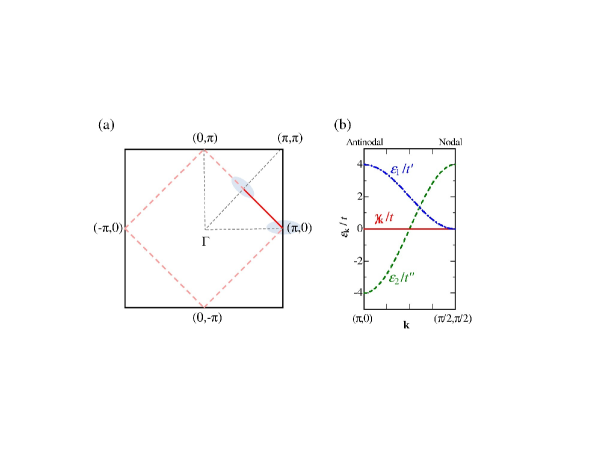
Figure 21: (Color online) (a) Bare Fermi surface at half filling in the tight-binding model with $t^{\prime}/t=0$ shown with a pink dashed line in the first Brillouin zone. The nodal $(\pi/2,\pi/2)$ and antinodal $(\pi,0)$ areas are marked by shadows. (b) Elements of bare band dispersion relations along $(\pi,0)\rightarrow(\pi/2,\pi/2)$: $\gamma_{\bf k}/t=-2(\cos k_{x}+\cos k_{y})$, $\varepsilon_{1}/t^{\prime}=-4\cos k_{x}\cos k_{y}$, and $\varepsilon_{2}/t^{\prime\prime}=-2(\cos 2k_{x}+\cos 2k_{y})$. $t^{\prime\prime}$ indicates the hopping integral to the third-neighbor sites ($\pm 2,0$) and ($0,\pm 2$), which is disregarded in this paper.

The source of this topological transition may have already arisen in the bare tight-binding dispersion or at the mean-field level. In Fig. 21(a), we show the Fermi surface at half filling for $t^{\prime}=0$, namely, the AF Brillouin zone boundary, on which $\tilde{\varepsilon}_{\bf k}=\gamma_{\bf k}=0$ as shown in Fig. 21(b) in red. If we add an infinitesimal diagonal hopping term [$\varepsilon_{1}({\bf k})$] (blue), the degeneracy on $(\pi,0)$–$(\pi/2,\pi/2)$ is lifted and the band maximum appears at $(\pi,0)$ or $(\pi/2,\pi/2)$ according to whether $t^{\prime}/t>0$ or $t^{\prime}/t<0$. As shown in green in Fig. 21(b), the third-neighbor hopping term $\varepsilon_{2}({\bf k})$ has a similar effect, if the sign of $t^{\prime\prime}$ is opposite the sign of $t^{\prime}$, although we do not treat it here. If we consider ordinary AF mean-field theory, the situation is similar because the quasi-particle dispersion

$$E^{\rm AF}_{\bf k}=\frac{U}{2}-\sqrt{\gamma_{\bf k}^{2}+\Delta_{\rm AF}^{2}}$$ (32)

is degenerate in the region $(\pi,0)$–$(\pi/2,\pi/2)$. When we add ${\cal H}_{t^{\prime}}$ as a perturbation to this framework, the leading difference in the dispersion relation is again $\langle\Phi_{\rm AF}|{\cal H}_{t^{\prime}}|\Phi_{\rm AF}\rangle\propto\varepsilon_{1}({\bf k})$. In these examples, the boundary of the topological change is at $t^{\prime}/t=0$. Nevertheless, it is not trivial whether this topological change is connected to the ones in strongly correlated cases (and even with a large $\delta$), and, if it is connected, why $t^{\prime}_{\rm L}/t$ slightly deviates to the negative side of $t^{\prime}/t$.

A topological change equivalent to the present result was found in the spectral function $A({\bf k},\omega)$ for the cases in which a few carriers are doped in the $t$-$t^{\prime}$-$J$ model and its extensions using various methods.[49, 50] In particular, Refs. SCBA and Nagaosa clearly argued, by means of a self-consistent Born approximation and a VMC method, respectively, that the location of the band maximum is different between hole- and electron-doped cases using typical parameters of cuprates. Actually, angle-resolved photoemission spectroscopy (ARPES) experiments revealed that the evolution of the Fermi surface with doping is different in hole-doped[53] and electron-doped[54] cases in lightly doped systems, in accordance with the results of the above theoretical study. Our result for the Hubbard model directly corresponds to these results for slightly doped $t$-$J$-type models.

As we will discuss in Sects. 6.2 and 6.3, this topological difference in the Fermi surfaces in $\Psi_{\rm AF}$ determines whether or not the $d$-wave SC order coexists with AF orders.

6 BRE on Mixed State of AF and SC Orders

In this section, we study a mixed state of AF and $d$-SC orders in a strongly correlated regime ($U>U_{\rm c}$):

$$\Psi_{\rm mix}={\cal P}\Phi_{\rm mix},$$ (33)

where $\varepsilon_{\bf k}^{\rm AF}$ and $\varepsilon_{\bf k}^{\rm SC}$ are independently optimized. In Sect. 6.1, we study the stability against phase separation (PS) and discuss whether charge fluctuation thereby correlates with the enhancement of $d$-SC. In Sect. 6.2, we consider the mechanism for the coexistence or mutual exclusivity of AF and $d$-SC orders. In Sect. 6.3, the notion treated in Sect. 6.2 is applied to the relationship between the staggered flux and $d$-SC states. In Sect. 6.4, we refer to the relationship between the pocket Fermi surfaces in the type-(ii) AF state and the Fermi arcs observed in the pseudogap phase of cuprates.

6.1 Stability against phase separation

Table 4: Relative and intrinsic stabilities of pure AF states and mixed states of AF and $d$-SC gaps obtained in recent studies using the Hubbard model summarized according to the level of BR and to whether $t^{\prime}/t\sim 0$ or $-0.3$. In the $U/t$ column, a typical target value is given. The first row denotes the range of finite AF orders. The second row indicates whether the system is homogeneous or phase-separated (P. S.). The third row for the mixed states shows whether AF and $d$-SC orders are coexisting or mutually exclusive (and the dominant order) in the main (or small-$\delta$) area of $m>0$.

Trial states	$U/t$	$t^{\prime}/t\sim 0$	$t^{\prime}/t\sim-0.3$	References
AF (no BR)	$8,12$	$\delta\lesssim 0.15$	no AF	Y2013
		P. S.	—
AF (BR)	$12$	$\delta\lesssim 0.16$	$\delta\lesssim 0.22$	proceedings1,proceedings2 &
		P. S.	homogeneous	this work
Mixed (no BR)		$\delta\lesssim 0.2$	—
	$10$	—	—	GL
		coexisting	—
Mixed (BR only		$\delta\lesssim 0.15$	$\delta\lesssim 0.15$
in SC)	$10$	P. S.	P. S.	Koba-old,Koba-ISS14
		coexisting	exclusive, AF
Mixed (BR in		$\delta\lesssim 0.16$	$\delta\lesssim 0.25$	proceedings3 &
AF & SC)	$12$	P. S.	homogeneous	this work
		coexisting	exclusive, AF
Mixed (many		$\delta\lesssim 0.18$	$\delta\lesssim 0.24$
parameters)	$10$	P. S.	homogeneous	Misawa
		coexisting	exclusive, AF

Before discussing $\Psi_{\rm mix}$, we refer to known aspects as to intrinsic stability of $\Psi_{\rm N}$, $\Psi_{d}$, and $\Psi_{\rm AF}$ against PS. Except for the limit of $\delta\rightarrow 0$, at which the anomaly of the Mott transition appears, the normal state $\Psi_{\rm N}$ is stable against PS.[29] As for $\Psi_{d}$, $E/t$ is a linear function of $\delta$ ($\chi_{\rm c}\rightarrow\infty$) for a small $\delta$, as we will discuss later, indicating that the stability against PS is marginal. However, this is distinct from the apparent instability of $\Psi_{\rm AF}$ toward PS. In the second row of Table 4, we summarize the conclusions of related VMC studies on the stability against PS of the AF and mixed states. The pure (not mixed) AF state is known to be unstable toward PS for $t^{\prime}/t\sim 0$[4, 29] but stable for $t^{\prime}/t\sim\pm 0.3$.[29] A mixed state in which BRE are introduced into $\varepsilon_{\bf k}^{\rm SC}$ but the AF part is fixed as $\varepsilon_{\bf k}^{\rm AF}=\gamma_{\bf k}$[20] exhibits instability toward PS for both $t^{\prime}/t=0$ and $-0.3$. To summarize, states with AF orders exhibit a tendency toward PS according to the value of $t^{\prime}/t$.

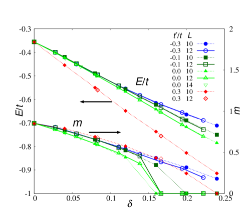
Figure 22: (Color online) Total energy per site and staggered magnetization (right axis) obtained for $\Psi_{\rm mix}$ with $U/t=12$ plotted as a function of doping rate. Data for four values of $t^{\prime}/t$ and $L=10$-$14$ are shown.

We study this property for $\Psi_{\rm mix}$ [Eq. (33)]. In Fig. 22, the total energy and sublattice magnetization [Eq. (29)] in $\Psi_{\rm mix}$ are shown as a function of the doping rate. First, we discuss the range in which the finite AF order occurs. As compared with the pure AF state $\Psi_{\rm AF}$,[29] the value of $\delta$ at which $m$ vanishes ($\delta_{\rm AF}$) is almost unchanging for $t^{\prime}/t=0$: $\delta_{\rm AF}\sim 0.16$, whereas $\delta_{\rm AF}$ somewhat increases for a large $|t^{\prime}/t|$. This small change in $\delta_{\rm AF}$ stems from the small energy difference between $\Psi_{\rm mix}$ and $\Psi_{\rm AF}$ (or $\Psi_{d}$), as shown in Table 3.

Table 5: Second-order coefficient $c_{2}$ estimated by the least-squares method for $E(\delta)/t$ [Eq. (34)] in the AF phase ($U/t=12$) of $\Psi_{\rm mix}$. For positive (negative) $c_{2}$, $\Psi_{\rm mix}$ is stable against (unstable toward) phase separation. Digits in round brackets indicate the error in the last digit.

$t^{\prime}/t$	$c_{2}$ ($L=10$)	$c_{2}$ ($L=12$)
$-0.4$	$2.42(8)~{}~{}$	—
$-0.3$	$1.85(9)~{}~{}$	$1.95(8)~{}~{}$
$-0.1$	$0.509(6)$	$0.323(8)$
$0.0$	$-0.551(5)$	$-0.553(7)$
$0.3$	$0.830(4)$	—

We turn to the stability against PS. This property is often judged by the sign of the charge compressibility $\kappa$ $[=(1-\delta)^{2}\chi_{\rm c}]$ or charge susceptibility $\chi_{\rm c}$ [$=(\partial^{2}E/\partial\delta^{2})^{-1}$]. For $\chi_{\rm c}>0$ ($\chi_{\rm c}<0$), the state is stable against (unstable toward) PS. Thus, we need to consider the $\delta$ dependence of $E/t$ (Fig. 22). Similarly to for $\Psi_{\rm AF}$,[29] we find for $\Psi_{\rm mix}$ that $E(\delta)/t$ is fitted well by the parabolic form

$$E(\delta)/t\simeq c_{0}+c_{1}\delta+c_{2}\delta^{2}$$ (34)

in the whole AF range ($\delta<\delta_{\rm AF}$); we have a unique value $\chi_{\rm c}=c_{2}^{-1}$ in the AF phase. The values of $c_{2}$ thus estimated for some values of $t^{\prime}/t$ and $L$ are summarized in Table 5. It reveals that $c_{2}$ (namely $\chi_{\rm c}$) becomes negative only for a narrow range near $t^{\prime}/t=0$, minutely $t^{\prime}_{\rm L}<t^{\prime}\lesssim 0.2t$ (see Fig. 27 later). This aspect is basically the same as that of the pure AF state.[29] Thus, the instability toward charge inhomogeneity originates in the AF order and is not directly connected with SC, as we will discuss shortly.

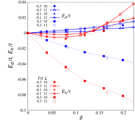
Figure 23: (Color online) Two elements [$E_{\rm d}$ (blue) and $E_{\rm h}$ (red)] of diagonal-hopping energy $E_{t^{\prime}}$ ($=E_{\rm d}+E_{\rm h}$) plotted as functions of doping rate for three values of $t^{\prime}/t$. Data for $L=10$ and $12$ with $U/t=12$ are shown.

Now, we identify the origin of the stability against PS for large values of $|t^{\prime}/t|$. First, we analyze $E/t$ by dividing it into its components $E_{U}/t$, $E_{t}/t$, and $E_{t^{\prime}}/t$. Because $E_{t}/t$ ($E_{U}/t$) is almost linear (somewhat convex) as a function of $\delta$ for any value of $t^{\prime}/t$ and $U>U_{\rm c}$ (not shown), these components do not contribute to phase stability. On the other hand, $E_{t^{\prime}}/t$ is concave for any $t^{\prime}/t$, but, of course, the degree of concavity diminishes as $|t^{\prime}/t|$ decreases and vanishes at $t^{\prime}/t=0$. We further analyze $E_{t^{\prime}}$ by dividing it into the two components $E_{\rm d}$ and $E_{\rm h}$ ($E_{t^{\prime}}=E_{\rm d}+E_{\rm h}$); $E_{\rm d}$ ($E_{\rm h}$) is the contribution of diagonal hopping that changes (does not change) the number of doublons.[4] In other words, $E_{\rm d}$ is generated by the creation or annihilation of D-H pairs, while $E_{\rm h}$ is generated by the hopping of doped (isolated) holes. In Fig. 23, we show the $\delta$ dependences of $E_{\rm d}$ and $E_{\rm h}$ for three values of $t^{\prime}/t$. We find that both $E_{\rm d}$ and $E_{\rm h}$ are concave but the curvature is much sharper for $E_{\rm h}$. To summarize, diagonal hopping ($t^{\prime}$ term), especially that of doped holes, brings about intrinsic stability against PS.

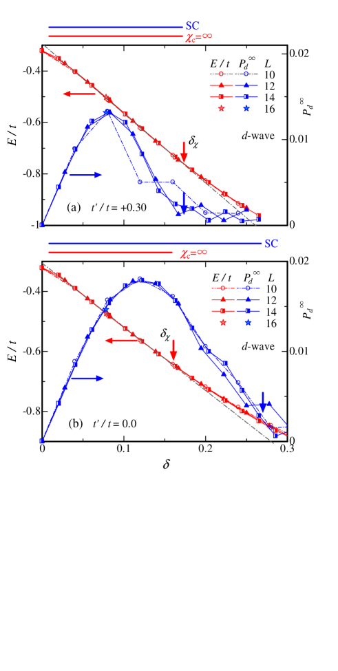
Figure 24: (Color online) Total energy and $d$-wave SC correlation function (right axis) obtained for $\Psi_{d}$ with $U/t=12$ plotted for (a) $t^{\prime}/t=0.3$ and (b) $t^{\prime}/t=0$ as functions of doping rate. Data for four values of $L$ are shown. Above each panel, the ranges of appreciable SC and where $\chi_{c}=\infty$ are shown. The straight dash-dotted line for $E/t$ is a guide for determining $\delta_{\chi}$.

A recent VMC study[5] argued that the increase in $\chi_{\rm c}$ has a one-to-one correspondence with the enhancement of SC order in the wave function used. We check this point for the present $\Psi_{d}$ and $\Psi_{\rm mix}$. First, we discuss the pure SC state, $\Psi_{d}$, whose $\delta$ dependence of $E/t$ for $t^{\prime}/t=0.3$ and $0$ is shown in Fig. 24. Aside from a Mott anomaly for $\delta\rightarrow 0$, $E/t$ becomes almost linear ($\chi_{\rm c}$ tends to diverge) for $\delta\lesssim\delta_{\rm\chi}$ (spinodal point), while $E/t$ becomes concave ($\chi_{\rm c}$ remains moderate) for $\delta>\delta_{\rm\chi}$. Note that $\chi_{\rm c}$ does not become negative unlike the case of $\Psi_{\rm AF}$. Such behavior of $E/t$ is preserved if $t^{\prime}/t$ is varied, but the range of $\chi_{\rm c}\rightarrow\infty$ shrinks as $t^{\prime}/t$ decreases; $\delta_{\rm\chi}\sim 0.17,0.15$, and $0.12$ for $t^{\prime}/t=0.3,0$, and $-0.3$, respectively. On the other hand, the SC correlation function exhibits the opposite behavior. As shown in Fig. 24, $P_{d}^{\infty}$ exhibits a well-known dome shape and the SC order is perceptible for $0<\delta<\delta_{\rm SC}$. Because the statistical fluctuation of $P_{d}^{\infty}$ becomes large for $\delta\sim\delta_{\rm SC}$, we estimate $\delta_{\rm SC}$ very roughly by the condition that the optimized gap parameter $\Delta_{d}/t$ becomes $0.03$ ($\Delta_{d}/t<0.03$ for $\delta>\delta_{\rm SC}$). We confirmed a known tendency that $\delta_{\rm SC}$ increases as $t^{\prime}/t$ decreases [for instance, see Fig. 25(d) in Ref. Y2013]; $\delta_{\rm SC}\sim 0.20,0.27$, and $0.31$ for $t^{\prime}/t=0.3,0$, and $-0.3$, respectively. Thus, the behaviors of $\delta_{\rm\chi}$ and $\delta_{\rm SC}$ as functions of $t^{\prime}/t$ are opposite; the increase in $\chi_{\rm c}$ rather has a negative correlation with the magnitude of SC in $\Psi_{d}$.

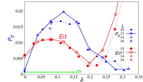
Figure 25: (Color online) Total energy (arbitrary unit) and $d$-wave SC correlation function obtained for $\Psi_{\rm mix}$ with $U/t=12$ and $t^{\prime}/t=0$ plotted as a function of doping rate. Instead of $E/t$, we plot $(E-\tilde{c_{0}}-\tilde{c_{1}}\delta)/t$ with $\tilde{c_{0}}$ and $\tilde{c_{1}}$ appropriately adjusted to emphasize the curvature of $E/t$. The area of finite staggered magnetization is shown by a green arrow.

Next, we consider the case of $\Psi_{\rm mix}$. As mentioned above, the range of $\chi_{\rm c}<0$ is included in the regime of type-(i) AF, $-0.05\lesssim t^{\prime}/t\lesssim 0.2$. As an example, we show in Fig. 25 the $\delta$ dependence of $E/t$ for $t^{\prime}/t=0$. We repeat that the area where $E/t$ is convex precisely coincides with that of finite $m$ ($\delta<\delta_{\rm AF}$) indicated by a green arrow. For $\delta>\delta_{\rm AF}$, where the state is SC, $E/t$ is concave. Furthermore, $P_{d}$ is smooth at $\delta=\delta_{\rm AF}$ and not specially enhanced in the area of $\chi_{\rm c}<0$. Anyway, as $\delta$ increases, after the AF order (or instability toward PS) vanishes at $\delta_{\rm AF}\sim 0.16$, SC survives up to $\delta_{\rm SC}\sim 0.27$ for $t^{\prime}/t=0$. In contrast, for $t^{\prime}/t=0.1$ [as in Fig. 26(a)], the SC first becomes weak at $\delta\sim 0.12$, but the area of $\chi_{\rm c}<0$ (and AF order) continues up to $\delta\sim 0.18$. The extents of $\delta$ where $\chi_{\rm c}<0$ and $P_{d}>0$ are reversed as $t^{\prime}/t$ varies.

Through the above analyses, we can conclude that the instability toward PS does not directly correlate with $d$-SC, although the ranges of $t^{\prime}/t$ where SC and PS arise are similar as seen in Fig. 27. As discussed in Refs. ZGRS and Y2013, we consider that the AF spin correlation and the suppression of charge fluctuation owing to the Mott physics are responsible for the behavior of the $d$-wave SC. We will return to this topic in Sect. 6.2.

Finally, we emphasize the importance of BRE again. As seen in Table 4, a mixed state in which BRE are considered only in $\varepsilon_{\bf k}^{\rm SC}$ exhibits instability toward PS even for $t^{\prime}/t=-0.3$.[20] In this mixed state, $\varepsilon_{\bf k}^{\rm AF}$ is fixed at $\gamma_{\bf k}$ [Eq. (13)], which resembles the optimized $\varepsilon_{\bf k}^{\rm AF}$ for $t^{\prime}/t=0$ ($t_{1}$, $t_{2}\sim 0$, see Fig. 13 for instance) belonging to the PS area. This means that the BRE on $\varepsilon_{\bf k}^{\rm AF}$ (independent of the BRE on $\varepsilon_{\bf k}^{\rm SC}$) are crucial for this property.

6.2 Coexistence or mutual exclusivity of AF and $d$-SC orders

Previous studies using various mixed states with BRE[16, 19, 20, 5] and a recent study using density matrix embedding theory (DMET)[7] argued that the orders of AF and $d$-SC are coexisting or mutually exclusive according to whether $t^{\prime}/t\sim 0$ or $t^{\prime}/t\lesssim-0.1$. Here, we systematically study this point for $\Psi_{\rm mix}$ and deduce the origin of the coexistence of the two orders, which is closely related to the mechanism of $d$-SC.

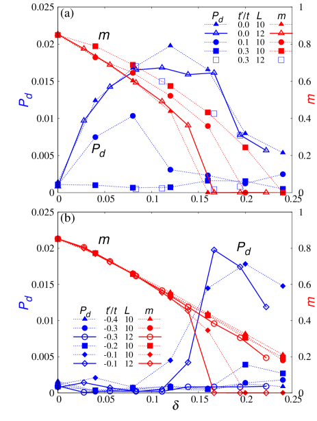
Figure 26: (Color online) Doping-rate dependence of $d$-wave SC correlation function $P_{d}$ (left axis) and staggered magnetization $m$ (right axis) shown for $U/t=12$. (a) Cases of $t^{\prime}>t^{\prime}_{\rm L}$ [type-(i) regime] and (b) those of $t^{\prime}<t^{\prime}_{\rm L}$ [type-(ii) regime] for both $L=10$ and $12$. The Lifshitz transition point of the pure AF state is $t^{\prime}_{\rm L}/t\sim-0.05$.

In Fig. 26, we show the $\delta$ dependence of the $d$-SC correlation function and staggered magnetization [Eq. (29)] measured in $\Psi_{\rm mix}$. For $\Psi_{\rm mix}$, we represent the $d$-SC correlation function by $P_{d}\equiv P_{d}({\bf R})$ [Eq. (22)] with ${\bf R}$ being the vector connecting the distant points in the system used [For instance, ${\bf R}=(5,5)$ for a system of $L=10$], because we focus on a strongly correlated regime (See Appendix C in Ref. Y2013). We show the results separately for the type-(i) AF and type-(ii) AF regimes in panels (a) and (b), respectively, because the features are distinct in the two regimes. In the type-(i) regime [panel (a)], the SC order ($P_{d}$) arises or vanishes regardless of whether the AF order ($m$) is present or absent. For example, for $t^{\prime}/t\sim 0$, AF and SC long-range orders coexist for $\delta<\delta_{\rm AF}$ and SC remains for $\delta_{\rm AF}<\delta<\delta_{\rm SC}$ as a pure SC order. On the other hand, in the type-(ii) regime [panel (b)], $P_{d}$ is almost zero for $\delta<\delta_{\rm AF}$ and grows after the AF order vanishes ($\delta>\delta_{\rm AF}$). Thus, the two orders are mutually exclusive. More accurately, in panel (b), a narrow range of coexistence exists near the boundary $\delta=\delta_{\rm AF}$ for small $|t^{\prime}/t|$, typically for $t^{\prime}/t=-0.1$. Anyway, the boundary between coexistence and mutual exclusivity is situated at $t^{\prime}=t_{\rm L}\sim-0.05t$, which is consistent with the previous results.[16, 19, 20, 5, 7] In the present results, it seems that the AF state is always more robust than the $d$-SC state and that the features of the underlying AF state control whether $d$-SC appears or not. We will return to these points shortly.

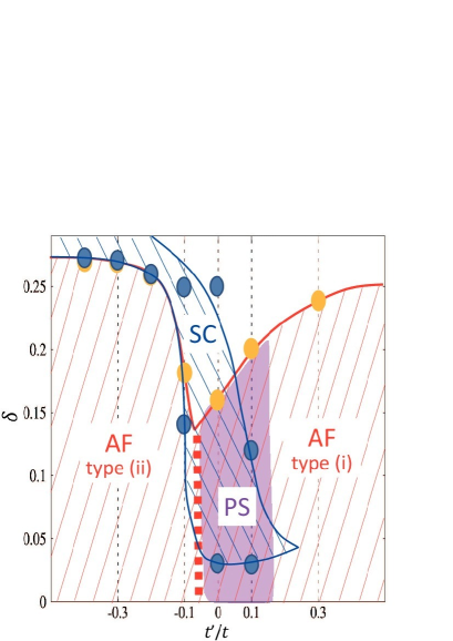
Figure 27: (Color online) Phase diagram in $\delta$-$t^{\prime}$ space for $U/t=12$ constructed for mixed state $\Psi_{\rm mix}$. The purple shaded area indicates the regime unstable toward phase separation, which is limited to within the type-(i) AF phase. The bold red dotted line indicates the Lifshitz transition boundary $t^{\prime}_{\rm L}/t$.

On the basis of the results for $\Psi_{\rm mix}$ above, we constructed the phase diagram in the $\delta$-$t^{\prime}$ space shown in Fig. 27. In accordance with Fig. 17 for the pure states, the AF state occupies a wide area. Except for the range of $-0.1\lesssim t^{\prime}/t\lesssim 0.2$, SC does not appear for low doping rates ($\delta\lesssim 0.2$). Furthermore, as mentioned, $\chi_{\rm c}$ becomes negative for $t^{\prime}_{\rm L}<t^{\prime}\lesssim 0.2t$. The state phase separates into an AF state at half filling and a state in the overdoped regime ($\delta\gtrsim 0.15$). Therefore, homogeneous SC does not appear in the underdoped regime for any value of $t^{\prime}/t$. This result greatly modifies the results of previous VMC studies without BRE, in which $d$-SC widely prevails for $t^{\prime}/t<0$, but is consistent with recent results of studies aapplying many-parameter VMC methods to Hubbard-type models[5] and a $d$-$p$ model[56] and a study employing DMET.[7] Such predominance of the long-range AF phase is inconsistent with the results of experiments on hole-doped cuprates as well as recent advanced studies on electron-doped cuprates.[57, 58, 59] We will discuss this point in Sect. 7.

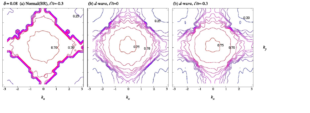
Figure 28: (Color online) Contour maps of $n({\bf k})$ at $U/t=12$ and $\delta\sim 0.08$ shown for (a)optimized normal (paramagnetic) state $\Psi_{\rm N}$ with $t^{\prime}/t=-0.3$ ($L=10$–$18$) and for (b) and (c) optimized pure $d$-wave pairing state $\Psi_{d}$ with $t^{\prime}/t=0$ (b) and $-0.3$ (c) ($L=10$–$16$).

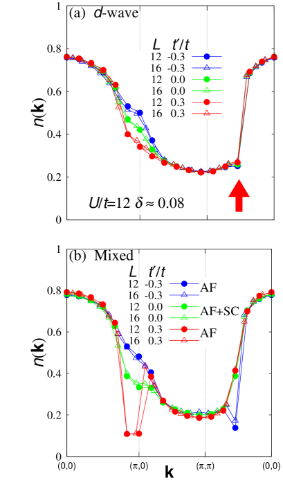
Figure 29: (Color online) Momentum distribution functions for (a) $d$-SC state and (b) mixed state for $U/t=12$ and $\delta\sim 0.08$ compared among three values of $t^{\prime}/t$. In (a), a nodal Fermi surface is indicated by an arrow. Data for $L=12$ and $16$ are plotted.

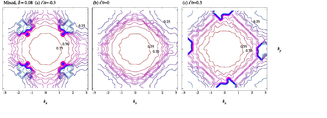
Figure 30: (Color online) Contour maps of $n({\bf k})$ for the optimized mixed state at $U/t=12$ and $\delta\sim 0.08$ shown for (a) $t^{\prime}/t=-0.3$, (b) $0$, and (c) $0.3$. The data in these maps include the data used in Fig. 29(b). Systems with $L=10$–$16$ are used.

Table 6: Locations of the centers of local Fermi surfaces in the state realized for a small $\delta$ (leftmost state for the mixed state) and $U/t=12$ summarized for the AF, $d$-SC, and mixed states. For the mixed state, the evolution of the realized states as $\delta$ increases is shown for $\delta\lesssim 0.3$. ‘Co’ (‘N’) indicates a coexisting state with AF and $d$-SC orders (normal state).

$t^{\prime}/t$	AF	$d$-SC	Mixed
			Evolution of state
$-0.3$	($\pi/2$, $\pi/2$)		AF(ii) $\rightarrow$ SC	($\pi/2$, $\pi/2$)
$-0.1$	($\pi/2$, $\pi/2$)	Always	AF(ii) $\rightarrow$ (Co) $\rightarrow$ SC	($\pi/2$, $\pi/2$)
$0.0$	($\pi$, $0$)	($\pi/2$, $\pi/2$)	Co $\rightarrow$ SC $\rightarrow$ N	No
$0.1$	($\pi$, $0$)		Co $\rightarrow$ AF(i) $\rightarrow$ N	No
$0.3$	($\pi$, $0$)		AF(i) $\rightarrow$ N	($\pi$, $0$)

Now, we consider why a $d$-SC order can coexist with a type-(i) AF order but is incompatible with a type-(ii) AF order. We can deduce the reason by considering the location of the Fermi surface in the underlying pure AF state. First, we review relevant properties of the $d$-SC state. In Figs. 28(b) and 28(c), we show contour maps of $n({\bf k})$ for $\Psi_{d}$ with $t^{\prime}/t=0$ and $t^{\prime}/t=-0.3$, respectively. The steep slope of $n({\bf k})$, indicative of a Fermi surface, exists only near $(\pm\pi/2,\pm\pi/2)$, and the gentle slopes around $(\pm\pi,0)$ and $(0,\pm\pi)$ indicate gaps, in contrast with the feature of the normal state shown in Figs. 28(a), which clearly exhibits a Fermi surface in any direction. In Fig. 29(a), $n({\bf k})$ in $\Psi_{d}$ [corresponding to Figs. 28(b) and 28(c)] is shown along the same path as in Fig. 19 for three values of $t^{\prime}/t$. As $t^{\prime}/t$ varies, $n({\bf k})$ around $(\pi,0)$ greatly varies but the nodal Fermi surface near $(\pi/2,\pi/2)$[21] is almost unchanging.[4] This indicates that the electronic states near $(\pi,0)$ are closely related to SC, because properties associated with SC such as $P_{d}$ greatly change with $t^{\prime}/t$. Actually, antinodal Fermi surfaces have the following advantages for $d$-SC on the square lattice:

(i) The density of states diverges at $(\pi,0)$ owing to a van Hove singularity for $|t^{\prime}/t|\leq 0.5$.

(ii) A $d$-SC gap $\Delta_{\bf k}$ with a similar form to Eq. (8) has a large magnitude at $(\pi,0)$.

(iii) The scattering of ${\bf q}=(\pi,\pi)$, which is induced by the AF exchange correlation between nearest-neighbor sites, is possible by connecting two antinodal points with opposite signs of $\Delta_{\bf k}$.

In Fig. 29(b), we plot $n({\bf k})$ obtained in $\Psi_{\rm mix}$ for the same parameter sets as in Fig. 29(a). Corresponding contour maps are displayed in Fig. 30. For $t^{\prime}/t=\pm 0.3$, the results for $\Psi_{\rm mix}$ are almost the same as those for $\Psi_{\rm AF}$ shown in Figs. 19(b) and 19(c) because the SC order does not appear. The results are also similar in Figs. 20(c) and 30(a) for $t^{\prime}/t=-0.3$. However, for $t^{\prime}/t=0$, where SC appears, the pocket Fermi surfaces at the antinodes in $\Psi_{\rm AF}$ in Fig. 19(b) are replaced with gap behavior (green) similar to the decreasing slope in $\Psi_{d}$ in Fig. 29(a). It is clearer to compare Fig. 20(b) for $\Psi_{\rm AF}$ with Fig. 30(b) for $\Psi_{\rm mix}$. This reveals that for the $d$-SC order, Fermi surfaces in the nodal directions are not necessary but gap formation in the antinodes is vital. Incidentally, the resultant SC in the coexisting state, if any, does not have a feature of cuprate SCs, namely, nodal Fermi surfaces [Fig. 29(b)]; it is smeared out by an AF gap. To provide an overview of this topic, we summarize in Table 6 the locations of the local Fermi surface centers of the three states for typical values of $t^{\prime}/t$. On the basis of this table with the above discussion, we may derive two requisites for $d$-SC in the mixed state:

(I) In the underlying pure AF (or normal) state, Fermi surfaces exist in the antinodes [around $(\pi,0)$ and equivalent points].

(II) The hot spots determined by $\varepsilon_{\bf k}^{\rm SC}$ (see Sect. 3.1) are situated in the Fermi surface area mentioned in (I).

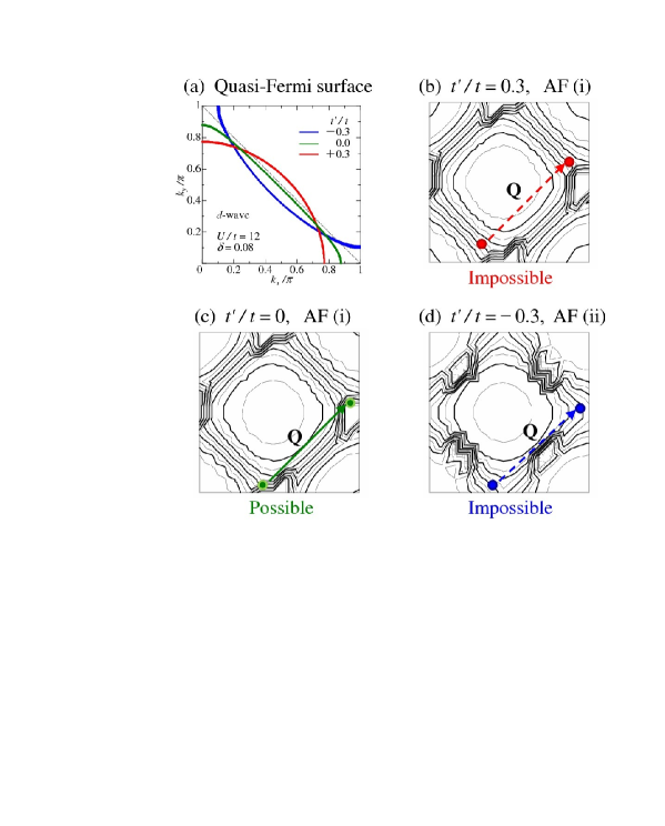
Figure 31: (Color online) (a) Quasi-Fermi surface in $\Psi_{d}$ obtained using $\varepsilon_{\bf k}^{\rm SC}$ in the first quadrant of the Brillouin zone for $U/t=12$ and $\delta=0.08$ for three typical values of $t^{\prime}/t$. The gray dash-dotted line indicates the AF Brillouin zone boundary. (b)-(d) Possibility of scattering of ${\bf q}={\bf Q}$ in $\Psi_{\rm mix}$ in the full Brillouin zone. The hot spots in the SC part are indicated by circles. Data for $\Psi_{\rm AF}$ with $U/t=12$ and $\delta=0.0816$ ($L=14$) are used to draw the contours.

On the basis of these conditions, we can explain the evolution of the states realized in $\Psi_{\rm mix}$ mentioned in Table 6. We show the main point schematically in Fig. 31. For $t^{\prime}<t^{\prime}_{\rm L}$, item (I) is not satisfied for a small $\delta$, and $d$-SC does not emerge as shown in Fig. 31(d). However, as $\delta$ approaches $\delta_{\rm AF}$, the edge of the Fermi surface centered at $(\pi/2,\pi/2)$ extends to the antinodes, as will be shown in Fig. 34(c). The scattering therein possibly yields a narrow window of coexistence, for example, for $t^{\prime}/t=-0.1$ [$\delta\sim 0.12$ and $\sim 0.139$ for $L=10$ and $12$, respectively] in Fig. 26(b). Regarding item (II), the hot spots stay near the antinodes in this range of $t^{\prime}/t$ [Fig. 31(a)]. On the other hand, for $t^{\prime}>t^{\prime}_{\rm L}$, item (I) is satisfied. For a small $|t^{\prime}/t|$, item (II) is also satisfied [Fig. 31(c)], so that a coexisting state appears as in Fig. 26(a). However, as $t^{\prime}/t$ increases, the hot spots shift toward the nodal area [red in Fig. 31(a)] and deviate from the Fermi surface range in the antinodes [Fig. 31(b)], which is relatively narrow as shown later in Fig. 35. Consequently, $d$-SC does not appear appreciably for $t^{\prime}/t=0.3$, as seen in Fig. 26(a). This behavior contrasts with that of the pure $d$-SC state (Fig. 24), in which $d$-SC becomes weak more slowly because the hot spots are always situated at the Fermi surface of the underlying state $\Psi_{\rm N}$, and the scattering intensity becomes weak as the hot spots move away from the antinodes.

To summarize, because the AF state underlies the $d$-SC order, substantial $d$-SC arises only when the scattering of ${\bf Q}$ in the antinodes is compatible with the AF behavior. The requisites for this are given by (I) and (II) above.

6.3 Coexistence of $d$-wave SC and staggered flux orders

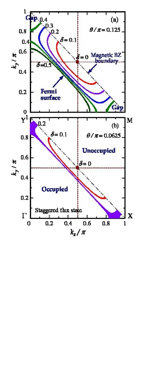
Figure 32: (Color online) Fermi surfaces of a staggered flux state for two values of $\theta$ and some doping rates drawn in the first quadrant of the Brillouin zone: $\Gamma=(0,0)$, ${\rm X}=(\pi,0)$, ${\rm M}=(\pi,\pi)$, and ${\rm Y}=(0,\pi)$. The thickness of the Fermi lines [e.g. for $\delta=0.2$ in (b)] indicates that $\varepsilon_{\bf k}^{\rm SF}$ is relatively flat.

To highlight the importance of Fermi surfaces in the antinodes for inducing a $d$-wave SC order, we consider the bare dispersion of a staggered flux (or $d$-density wave) state.[3, 47] Although this state has been extensively studied as a candidate for the pseudogap state as well as the ground state of cuprates, here we avoid referring to various interesting aspects of this state and focus on its bare dispersion:

$$\varepsilon_{\bf k}^{\rm SF}=-2t\sqrt{\cos^{2}{k_{x}}+2\cos{2\theta}\cos{k_{x}}\cos{k_{y}}+\cos^{2}{k_{y}}},$$ (35)

where $\theta$ corresponds to a quarter of the magnetic flux penetrating each plaquette of the square lattice and is treated as a variational parameter here. For $\theta=0$, $\varepsilon_{\bf k}^{\rm SF}$ is reduced to $\gamma_{\bf k}$ [Eq. (13)]; for $\theta=\pi/4$ ($\pi$-flux state), $\varepsilon_{\bf k}^{\rm SF}$ at half filling yields a Dirac cone with a linear dispersion with apices at $(\pm\pi/2,\pm\pi/2)$. In Fig. 32, we show the Fermi surfaces generated by $\varepsilon_{\bf k}^{\rm SF}$ in the first quadrant of the Brillouin zone for two values of $\theta$ and some values of $\delta$ for each $\theta$. At half filling, the Fermi surface is the apex of an elongated Dirac cone at $(\pi/2,\pi/2)$. For $\delta>0$, a Fermi surface appears as a slice of an elongated Dirac cone around the nodal point $(\pi/2,\pi/2)$. Gaps open in the antinodes around ($\pi,0$) and ($0,\pi$). The form of the pocket Fermi surfaces and the antinodal gaps resembles the features in the pseudogap phase of cuprates. Note that the pocket Fermi surface becomes slender and its edge approaches the antinodes as $\theta$ decreases and/or $\delta$ increases.

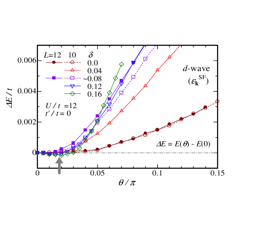
Figure 33: (Color online) Difference in total energy upon introducing a staggered flux $4\theta$ in $\varepsilon^{\rm SF}_{\bf k}$ [Eq. (35)] for $U/t=12$ and $t^{\prime}/t=0$. The thick arrow indicates the minimum (at $\theta/\pi\sim 0.02$) for $\delta=0.16$.

Here, we study how the energy in $\Psi_{d}$ [Eq. (19)] varies when we use $\varepsilon_{\bf k}^{\rm SF}$ instead of $\gamma_{\bf k}$ as $\varepsilon_{\bf k}^{\rm SC}$. If the coexistence of staggered flux and $d$-wave SC orders is favored, the energy in $\Psi_{d}$ may be reduced by a finite value of $\theta$. In Fig. 33, we show the increment in energy per site $\Delta E$ as compared with that in $\Psi_{d}$ with $\gamma_{\bf k}$ as a function of $\theta$ for $t^{\prime}/t=0$ and $U/t=12$. For large values of $\theta$ ($\gtrsim 0.05\pi$), the energy markedly increases regardless of $\delta$. On the other hand, for a small $\theta$ and large $\delta$, $\Delta E$ is small or slightly negative, as indicated by the arrow, meaning that the two orders possibly coexist. In these cases, the Fermi surfaces reach the antinodes. This is consistent with the notion that the gap in the antinodes in $\varepsilon_{\bf k}$ for the underlying state is unfavorable to the $d$-SC order. To summarize, a robust staggered flux order and a $d$-wave SC order are unlikely to coexist, although, to ensure this conclusion, we should investigate an appropriate mixed state of the two orders.

6.4 Possible relation with pseudogap

One of the anomalous features arising in the pseudogap phase ($T_{\rm c}<T<T^{*}$) of underdoped cuprates is the Fermi arcs[60] observed in ARPES spectra, namely, unclosed Fermi surfaces whose centers are situated in the nodal directions near $(\pm\pi/2,\pm\pi/2)$, and similarly Fermi surface pockets[61, 62]. If $T$ is fixed, a Fermi arc becomes longer as $\delta$ increases and becomes connected to other arcs in adjacent quadrants of the Brillouin zone to form an ordinary closed Fermi surface at the phase boundary ($T=T^{*}$). The origin of the pseudogap has not yet been elucidated. First, as a possible candidate for the Fermi arc, we consider the pocket Fermi surface of a doped $\Psi_{\rm AF}$.

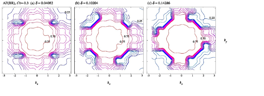
Figure 34: (Color online) Contour maps showing the evolution of $n({\bf k})$ as the doping rate increases in the type-(ii) AF state for $t^{\prime}/t=-0.3$ ($U/t=12$). Three typical doping rates are selected. Data for $L=14$ are used.

As shown in Fig. 20(c), a pocket Fermi surface of a type-(ii) AF state is formed around $(\pi/2,\pi/2)$ and is similar to the Fermi arc observed by ARPES. $\Psi_{\rm AF}$ has energy gaps around the antinodes in the sense that $n({\bf k})$ is smooth with a finite $|\nabla n({\bf k})|$. In Fig. 34, we show contour maps of $n({\bf k})$ for different doping rates, where the other conditions are the same ($t^{\prime}/t=-0.3$, $U/t=12$). This figure reveals how the pocket Fermi surface evolves as $\delta$ increases; a small pocket Fermi surface appears around $(\pi/2,\pi/2)$ for very light doping, the arc length becomes long along the AF Brillouin zone boundary $(\pi,0)$–$(0,\pi)$, finally forming a connected Fermi surface centered at $\Gamma=(0,0)$ for $\delta=0.2245$ (not shown), where the AF order vanishes. This behavior is consistent with that of the Fermi arc of cuprates. For the appearance of such behavior at a finite temperature, it is also important that the type-(ii) $\Psi_{\rm AF}$ has a very low energy and is stable against phase separation. Furthermore, the type-(ii) $\Psi_{\rm AF}$ does not coexist with $d$-SC except for $\delta\sim\delta_{\rm AF}$. Although this result cannot be directly applied to the pseudogap phase of cuprates because an AF long-range order has not been observed, it is intriguing that short-range AF orders of $20$-$30$ lattice constants were observed up to high temperatures.[8]

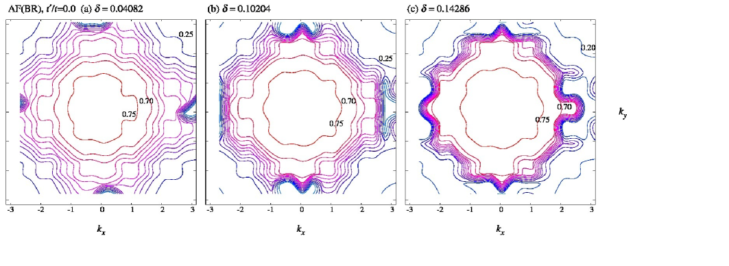
Figure 35: (Color online) Contour maps showing the evolution of $n({\bf k})$ as the doping rate increases in the type-(i) AF state for $t^{\prime}/t=-0.3$ ($U/t=12$). Data for the same doping rates as in Fig. 34 are displayed for comparison. Systems with $L=14$ are used.

In Fig. 35, we show the evolution of contour maps of $n({\bf k})$ as $\delta$ increases in the type-(i) AF state ($t^{\prime}/t=0$). In contrast to the type-(ii) AF state, a pocket Fermi surface grows from the antinodes in the nodal directions and finally forms a closed Fermi surface centered at $\Gamma=(0,0)$ for $\delta=0.1633$ (not shown). Because energy gaps open for $\delta<\delta_{\rm AF}$ in the nodal directions, the type-(i) AF state, which corresponds to electron-doped cuprates, is not directly related to the Fermi arc phenomena.

7 Summary and Discussion

In this paper, we studied band renormalization effects (BRE) owing to electron correlation on a mixed state of $d_{x^{2}-y^{2}}$-wave pairing ($d$-SC) and antiferromagnetic (AF) orders, as well as normal (paramagnetic), pure $d$-SC, and pure AF states, by applying a variational Monte Carlo (VMC) method to the Hubbard ($t$-$t^{\prime}$-$U$) model. For the mixed state, BRE were introduced into the AF and $d$-SC parts independently; BRE on AF orders, previously not investigated,[28] markedly change the previous knowledge of the Hubbard model. By searching widely in the model-parameter space with wave functions on various levels, we obtained systematic insights, particularly into the following subjects: (A) Ground-state phase diagrams in the space of $U/t$, $t^{\prime}/t$, and $\delta$. (B) In what regime and through what mechanisms does the coexistence of AF and $d$-SC arise? (C) In what regime and from what cause does instability toward inhomogeneous phases occur? First, we itemize the main results in this work:

(1) In the $d$-SC state, the effective band $\varepsilon_{\bf k}^{\rm SC}$ is markedly renormalized for the model parameters of $U/t\gtrsim 6$, a large $|t^{\prime}/t|$, and a small $\delta$ $(\lesssim 0.1)$ (Figs. 4 and 5), as known previously. We found, however, owing to BRE, not only is the improvement in energy much smaller than those in the normal and AF states, but also quantities related to SC [$P_{d}$, $S({\bf q})$, $n({\bf k})$] are modified only very slightly (Figs. 6-8).

(2) In the normal state, BRE apply $U\gtrsim U_{\rm c}$, $\delta\lesssim 0.05$, and $|t^{\prime}/t|\gtrsim 0.1$ with $U_{\rm c}/t$ being the Mott transition point (Fig. 10). The improvement in energy is an order of magnitude larger than that of the $d$-SC state but an order of magnitude smaller than that of the AF state (Fig. 11).

(3) In all the states studied, band renormalization takes place to reduce the kinetic energy ($E_{t}$) at the cost of the interaction energy ($E_{U}$), which corresponds to the tendency of a strongly correlated state to undergo a phase transition to reduce the kinetic energy.[35, 4] In the resultant renormalized band, the nesting condition tends to be restored ($t_{1}/t\rightarrow 0$).

(4) For the AF state, BRE are useful in reducing the energy, especially for $t^{\prime}/t<0$ (Fig. 14); the qualitative features are almost independent of $U/t$ for $U>U_{\rm AF}$. As a result, the AF state occupies a wide area ($\delta\lesssim 0.2$) in the phase diagrams (Figs. 17 and 27). The AF area is considerably wider for $t^{\prime}/t=-0.3$ than for $t^{\prime}/t=0$, which contrasts with the results without BRE. In a doped metallic AF state, as $t^{\prime}/t$ is varied, a kind of first-order Lifshitz transition takes place at $t^{\prime}=t_{\rm L}\sim-0.05t$ regardless of the values of $U/t$ and $\delta$. In the type-(i) [(ii)] AF regime ($t^{\prime}>t_{\rm L}$) [($t^{\prime}<t_{\rm L}$)], local pocket Fermi surfaces arise around $(\pi,0)$ [$(\pi/2,\pi/2)$] and equivalent points (Figs. 19 and 20). This difference plays a critical role in inducing the $d$-SC mentioned in (6) before. The Fermi surface in the type-(ii) AF is possibly related to the Fermi arcs found in cuprates.

(5) In the mixed state, the range of instability toward phase separation (PS) is found to be $t^{\prime}_{\rm L}/t<t^{\prime}/t\lesssim 0.2$, similarly to in the AF states.[4, 29] The AF order is responsible for this instability, which does not directly correlate with $d$-SC. Elsewhere, the state is stable against PS. This stability is mainly due to the diagonal hopping of doped carriers.

(6)The coexistence or mutual exclusivity of AF and $d$-SC orders was studied in the mixed state (Fig. 26). The AF order has preferentially exhibits this property because the AF part greatly reduces the energy compared with the SC part (Fig. 16). By checking various cases, we found two requisites for the $d$-SC order to arise (Fig. 31): (i) In the underlying pure AF (or normal) state, Fermi surfaces exist in the antinodes [near $(\pi,0)$ and equivalent area]. (ii) The hot spots determined by $\varepsilon_{\bf k}^{\rm SC}$ are situated in the Fermi surface area. These requisites indicate that the scattering of ${\bf q}=(\pi,\pi)$ in the antinodes is vital for $d$-SC. Thus, the coexistence basically occurs in the type-(i) AF regime. The range of $t^{\prime}/t$ in which coexistence occurs is similar to that for the instability toward PS (Fig. 27), but this similarity is accidental. These requisites seem to apply to the coexistence of $d$-SC and staggered flux orders.

The present results are quantitatively consistent with recent studies with advanced techniques,[5, 6, 7] and make it possible to reasonably interpret individual features of previous studies.

Finally, we discuss the relationship with cuprates. The present results that the AF order is predominant for a wide range of model parameters ($U/t\gtrsim 6$, $\delta\lesssim 0.2$, most $t^{\prime}/t$) and that uniform $d$-SC disappears in the underdoped regime are consistent with those of recent VMC,[5] DMFT,[6] and DMET[7] studies based on the Hubbard model. Furthermore, recent VMC studies on the $t$-$J$[63] and $d$-$p$[56] models display the same tendency. Nevertheless, these results are inconsistent with properties common to hole-doped cuprate SCs: the AF long-range order is broken by less than 5% doping with carriers and high-$T_{\rm c}$ $d$-SC appears in the underdoped regime. In addition, it was recently shown that well-annealed electron-doped samples with small doping rates (5-10%) exhibit no AF long-range orders but metallic or SC behavior[57, 58] with entirely closed Fermi surfaces.[59] Assuming that the AF order is excluded for some reason, most properties of the remaining $d$-SC derived by theories so far are basically consistent with those of cuprates. Thus, it is important to clarify why AF long-range order is robust in the theory. It seems that the approximations applied are not responsible for the predominant AF orders, but the models are lacking in certain important factors that destabilize AF orders. They are possibly disorders or impurities inherent in cuprate SCs. It seems that theoretical research on cuprate SCs may proceed to this direction.

After the submission of this paper, we noticed that BRE on AF states were already considered in a VMC study of Watanabe, Shirakawa and Yunoki for three-band as well as single-band Hubbard models.[64] They used the optimization method mentioned as ‘an alternative approach’ in Appendix B. Their results are basically consistent with ours.

We thank Kenji Kobayashi, Masao Ogata, Shun Tamura, Junya Otsuki, Yuta Toga, Hiroshi Watanabe, Kentaro Sato, and Masaki Fujita for useful discussions and information. This work was supported in part by Grants-in-Aid from the Ministry of Education, Culture, Sports, Science and Technology, Japan.

Appendix A Details of Optimization in Normal State

In this Appendix, we explain how to actually deal with the BR of the normal (paramagnetic) state $\Psi_{\rm N}$ [Eq. (26)] for finite-size systems. As mentioned in Sect. 2, $\Psi_{\rm N}$ depends only on the choice of $\{{\bf k}\}_{\rm occ}$ (Fermi surface) and not explicitly on $\varepsilon_{\bf k}$. In the thermodynamic limit ($L=\infty$), where ${\bf k}$ is a continuous variable, $\{{\bf k}\}_{\rm occ}$ continuously changes as $\varepsilon_{\bf k}$ or the band parameters therein ($t_{1}/t$, etc.) gradually vary. This means that $\{{\bf k}\}_{\rm occ}$ directly depends on the band parameters. On the other hand, in the finite systems we treat here, for which the available ${\bf k}$ are discrete, $\{{\bf k}\}_{\rm occ}$ (namely $\Psi_{\rm N}$) is invariable in a certain range of band parameters (or $\varepsilon_{\bf k}$) and discontinuously changes at the edges of the range. Generally, this range becomes wider for a smaller $L$. To begin with, we illustrate this point assuming that the effective band is given by $\varepsilon_{\bf k}^{\rm N}$ in Eq. (5). Even for this simple form of $\varepsilon_{\bf k}$, we believe that full BRE are achieved in most cases.

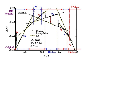
Figure 36: (Color online) Illustration of how to obtain the band-renormalized energy in $\Psi_{\rm N}$ within a single variational band parameter $t_{1}/t$ for a specific model parameter set ($L=10$, $\delta=0.08$, $U/t=12$). The total energy per site is plotted as a function of $t^{\prime}/t$ ($<0$). For details, see text.

To avoid confusion between $t^{\prime}/t$ in ${\cal H}$ (model parameter) and the variational band parameter $t_{1}/t$ in $\Psi_{\rm N}$, we start with the noninteracting case ($U=0$). In this case, the exact ground state is given by Eq. (4), in which $\{{\bf k}\}_{\rm occ}$ is determined by the bare band dispersion $\tilde{\varepsilon}_{\bf k}$ in Eq. (2), indicating that $t_{1}=t^{\prime}$ and $\varepsilon_{\bf k}=\tilde{\varepsilon}_{\bf k}$ for $U=0$ in variation theory. If we decrease the sole band parameter $t^{\prime}/t$ in ${\cal H}$ from zero, $\{{\bf k}\}_{\rm occ}$ is switched from one configuration to another at certain discrete values of $t^{\prime}/t$. In Fig. 36, we show such evolution of $\{{\bf k}\}_{\rm occ}$, for $L=10$ and $\delta=0.08$ as an example, with alternate red and blue arrows near the lower horizontal axis; $\{{\bf k}\}_{\rm occ}$ is switched as

$$\{{\bf k}_{\rm 0}\}_{\rm occ}\rightarrow\{{\bf k}_{\rm 1}\}_{\rm occ}\rightarrow\{{\bf k}_{\rm 2}\}_{\rm occ}\rightarrow\{{\bf k}_{\rm 3}\}_{\rm occ}\rightarrow\cdots$$ (36)

at $t^{\prime}/t\sim-0.107$, $-0.137$, $-0.213$, $-0.357$, $\cdots$. Let A_ℓ ($\ell$: integer) denote the area of $t^{\prime}/t$ where $\{{\bf k}\}_{\rm occ}=\{{\bf k}_{\ell}\}_{\rm occ}$ as shown in Fig. 36, for example, A${}_{2}=[-0.213,-0.137]$. Note that within each A_ℓ, the ground-state wave function $\Psi_{\rm N}$ (=$\Phi_{\rm N}$) is unchanging but the energy changes with $t^{\prime}/t$ owing to the diagonal hopping term.

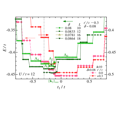
Figure 37: (Color online) Energy expectation values of the normal state $\Psi_{\rm N}$ for some model-parameter sets ($L$, $\delta$, $t^{\prime}/t$, $U/t=12$) plotted as functions of the band parameter $t_{1}/t$. The data with light-green diamonds and lettering A_ℓ correspond to the set discussed in the text ($10$, $0.08$, $-0.3$, $12$). Those plotted as dark circles are identical to those shown in Fig. 16.

Next, we consider interacting cases ($U>0$). Let the model parameters be fixed, for example, at $L=10$, $\delta=0.08$, $t^{\prime}/t=-0.3$, and $U/t=12$. For such a parameter set, we need to optimize $\Psi_{\rm N}$ by adjusting the band parameter $t_{1}/t$ independently of $t^{\prime}/t$ together with the correlation parameters. Because $\Phi_{\rm N}$ in Eq. (4) depends only on $\{{\bf k}_{\ell}\}_{\rm occ}$ but not directly on $t_{1}/t$, $\Psi_{\rm N}$ should exhibit completely flat energy as a function of $t_{1}/t$ in A_ℓ and discontinuities at the edges of A_ℓ. Actually, in Fig. 37, we show the $t_{1}/t$ dependence of the total energy for the above parameter set with light-green diamonds, along with the same quantity for other parameter sets. Because the effective band dispersion $\varepsilon^{\rm N}_{\bf k}$ [Eq. (5)] in $\Psi_{\rm N}$ is assumed to be the same form as the bare band dispersion $\tilde{\varepsilon}_{\bf k}$ [Eq. (2)],[65] the division of the areas (A_ℓ) for $t^{\prime}/t$ discussed above directly corresponds to the division of $t_{1}/t$, as also marked by A_ℓ in Fig. 37. The energy minimum for the above model parameter set ($t^{\prime}/t=-0.3$) is obtained not in A₃ (including $t_{1}/t=-0.3$) but in A₂, meaning that BRE manifest themselves.

Owing to this locally flat behavior of $E/t$, ordinary optimization techniques that need information about gradients of $E/t$ are inapplicable to $\Psi_{\rm N}$. Here, we use another way of optimization. Below, we describe its outline with an illustration in Fig. 36 for a model-parameter set ($L=10$, $\delta=0.08$, $U/t=12$) as an example. (i) Calculate the total energy $E/t$ densely as a function of $t^{\prime}/t$ for a fixed set of the other parameters ($L$, $\delta$, $U/t$) without introducing BRE, namely by putting $t_{1}=t^{\prime}$. In Fig. 36, the $E/t$ thus obtained are plotted with small solid circles with a thick dashed line. We find that $E/t$ is described by a distinct nearly straight curve for each A_ℓ. (ii) Each segmented curve (say in A_ℓ) can be well extrapolated using a first- or second-order least-squares method:

$$E_{\ell}(t^{\prime}/t)=c^{(\ell)}_{0}+c^{(\ell)}_{1}(t^{\prime}/t)+c^{(\ell)}_{2}(t^{\prime}/t)^{2}.$$ (37)

The extrapolated curves are shown with thin dashed lines in Fig. 36 and practically coincide with the values of $E/t$ actually calculated with $\{{\bf k}_{\ell}\}_{\rm occ}$ (BRE) outside A_ℓ, whose values are shown with open circles joined by thin dull-green curves. Therefore, we may substitute such extrapolated values for the results of actual BRE calculations to save labor. (iii) The optimized energy allowing for BRE for a fixed value of $t^{\prime}/t$ is given by the lowest extrapolated value among the all the A_ℓ. For $t^{\prime}/t=-0.3$, for example, the lowest energy is given by $\{{\bf k}_{2}\}_{\rm occ}$, and the improvement in energy owing to BRE ($\Delta E/t$) is indicated by a brown arrow. We actually estimated the optimized BRE energies of $\Psi_{\rm N}$ for most model parameter sets through this procedure. To obtain other quantities, however, calculations using the optimized parameters are necessary.

Under the upper horizontal axis in Fig. 36, we show the areas of $\{{\bf k}_{\ell}\}_{\rm occ}$ which yield the optimized $E/t$ with red and blue arrows. It reveals that these areas of $\{{\bf k}_{\ell}\}_{\rm occ}$ with BRE often deviate from the areas of $\{{\bf k}_{\ell}\}_{\rm occ}$ for bare cases shown near the lower horizontal axis. Thus, in this model parameter set, the energy reduction owing to BRE is brought about discontinuously as a function of $t^{\prime}/t$ [see Fig. 10(b)]. In Fig. 16, we actually illustrate the above process of optimization associated with BRE for $\Psi_{\rm N}$ with $L=12$, $\delta=0.0833$, and $U/t=12$. The red line indicates the optimized line for $\Psi_{\rm N}$. In this parameter, BRE are ineffective for or small $-0.573\lesssim t^{\prime}/t\lesssim 0.343$.

Appendix B Details of Optimizing AF and Mixed States

In optimizing $\Psi_{\rm AF}$ and $\Psi_{\rm mix}$, a similar difficulty exists in the case of $\Psi_{\rm N}$. Namely, if we determine $\{\bf k\}_{\rm occ}^{\rm AF}$ according to $\varepsilon_{\bf k}^{\rm AF}$, as $t_{\eta}$ is gradually varied, total energy $E/t$ discontinuously changes at a value where $\{\bf k\}_{\rm occ}^{\rm AF}$ is switched to another configuration. In contrast to $\Psi_{\rm N}$, we have to optimize $\varepsilon_{\bf k}^{\rm AF}$ in addition to $\{\bf k\}_{\rm occ}^{\rm AF}$ for $\Psi_{\rm AF}$ and $\Psi_{\rm mix}$, as shown in Table 1. What is worse, $E/t$ depends on $t_{\eta}$ only very weakly. For this reason, the stochastic reconfiguration method and quasi-Newton methods did not work effectively, and we returned to a primitive linear optimization method in most cases.

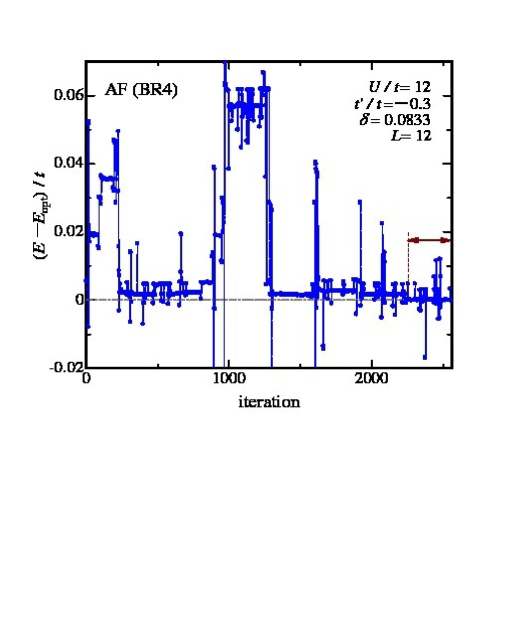
Figure 38: (Color online) Evolution of the energy expectation value in $\Psi_{\rm AF}$ obtained by VMC process using a simple linear optimization method. The results of eight calculations successively performed are plotted in sequence, in each of which 320 linear optimizations were carried out. The initial parameter values in each calculation were set to those that yielded the lowest plateau energy in the previous calculations. We estimated the optimized energy, in this case, by averaging the final results indicated by the arrow. In averaging, we exclude scattered data that are more than twice the standard deviation from the mean.

We show an example of optimizing $\Psi_{\rm AF}$ in Fig. 38, where the expectation value of $E/t$ obtained in each linear optimization of the parameters is plotted for the specified model parameter set. Typically, $2.5\times 10^{5}$ samples are used for the linear optimization. The expectation value of $E$ does not monotonically decrease to the optimized value $E_{\rm opt}$ but irregularly fluctuates, exhibiting wide and narrow plateaus and irrelevant spikes. A given configuration $\{\bf k\}_{\rm occ}^{\rm AF}$ yields a plateau or plateaus with the same $E$. We determined $E_{\rm opt}$ by averaging $E$ in the lowest plateau and checking that the estimated value is smoothly connected to those of other model parameter sets. For $t^{\prime}\sim t^{\prime}_{\rm L}$, the statistical fluctuations become very large because multiple $\{\bf k\}_{\rm occ}^{\rm AF}$ have a value of $E$ comparable to $E_{\rm opt}$. Therefore, in this regime, we carried out up to fifty calculations for a single model-parameter set, especially for $\Psi_{\rm mix}$.

As an alternative approach, we may optimize $\Psi_{\rm AF}$ and $\Psi_{\rm mix}$ with a fixed $\{\bf k\}_{\rm occ}^{\rm AF}$ using the stochastic reconfiguration method. By carrying out such operations for various values of $\{\bf k\}_{\rm occ}^{\rm AF}$, we can single out the $\Psi$ with the lowest $E/t$. Because the number of choices of $\{\bf k\}_{\rm occ}^{\rm AF}$ rapidly increases as $L$ increases, we may adopt the way of choosing $\{\bf k\}_{\rm occ}$ used for $\Psi_{\rm N}$ in AppendixA. Anyway, the task of optimizing $\Psi_{\rm AF}$ and $\Psi_{\rm mix}$ is much more burdensome than that for $\Psi_{d}$.

References

- [1] J. G. Bednorz and K. A. Müller, Z. Phys. B 64, 189 (1986).
- [2] For the recent status of experimental research, see, for instance, articles in the special issue of J. Phys. Soc. Jpn. 81 vol. 1 (2012) on “Recent developments in superconductivit”.
- [3] For the - model, see P. A. Lee, N. Nagaosa, and X.-G. Wen, Rev. Mod. Phys. 78, 17 (2006); M. Ogata and H. Fukuyama, Rep. Prog. Phys. 71, 036501 (2008). For the Hubbard model, see, for instance, Table I in Ref. \citenMisawa.
- [4] H. Yokoyama, M. Ogata, Y. Tanaka, K. Kobayashi, and H. Tsuchiura, J. Phys. Soc. Jpn. 82, 014707 (2013).
- [5] T. Misawa and M. Imada, Phys. Rev. B 90, 115137 (2014).
- [6] J. Otsuki, H. Hafermann, and A. I. Lichtenstein, Phys. Rev. B 90, 235132 (2014).
- [7] B.-X. Zheng and G. K.-L. Chan, Phys. Rev. B 93, 035126 (2016).
- [8] Y. Sidis, C. Ulrich, P. Bourges, C. Bernhard, C. Niedermayer, L. P. Regnault, N. H. Andersen, and B. Keimer, Phys. Rev. Lett. 86, 4100 (2001); H. A. Mook, Pengcheng Dai, S. M. Hayden, A. Hiess, J. W. Lynn, S.-H. Lee, and F. Dogan, Phys. Rev. B 66, 144513 (2002); J. A. Hodges, Y. Sidis, P. Bourges, I. Mirebeau, M. Hennion, and X. Chaud, Phys. Rev. B 66, 020501(R) (2002).
- [9] M. Capone and G. Kotliar, Phys. Rev. B 74, 054513 (2006).
- [10] D. Sénéchal, P.-L. Lavertu, M.-A. Marois, and A.-M. S. Tremblay, Phys. Rev. Lett. 94, 156404 (2005).
- [11] M. Aichhorn, E. Arrigoni, M. Potthoff, and W. Hanke, Phys. Rev. B 76, 224509 (2007).
- [12] S. S. Kancharla, B. Kyung, D. Sénéchal, M. Civelli, M. Capone, G. Kotliar, and A.-M. S. Tremblay, Phys. Rev. B 77, 184516 (2008).
- [13] T. K. Lee and S. Feng, Phys. Rev. B 38, 11809 (1988).
- [14] A. Himeda and M. Ogata, Phys. Rev. B 60, R9935 (1999).
- [15] D. A. Ivanov, Phys. Rev. B 70, 104503 (2004).
- [16] C. T. Shih, Y. C. Chen, C. P. Chou, and T. K. Lee, Phys. Rev. B 70, 22502(R) (2004); C. T. Shih, J. J. Wu, Y. C. Chen, C. Y. Mou, C. P. Chou, R. Eder, and T. K. Lee, Low Temp. Phys. 31, 757 (2005).
- [17] S. Pathak, V. B. Shenoy, M. Randeria, and N. Trivedi, Phys. Rev. Lett. 102, 027002 (2009).
- [18] T. Giamarchi and C. Lhuillier, Phys. Rev. B 43, 12943 (1991).
- [19] K. Kobayashi and H. Yokoyama, J. Phys. Chem. Solids 69, 3274 (2008); Physica C 469, 974 (2009).
- [20] K. Kobayashi and H. Yokoyama, JPS Conf. Proc. 1, 012120 (2014); JPS Conf. Proc. 3, 015012 (2014); Phys. Proc. 58, 22 (2014); Phys. Proc. 65, 9 (2015).
- [21] A. Himeda and M. Ogata, Phys. Rev. Lett. 85, 4345 (2000).
- [22] C. T. Shih, T. K. Lee, R. Eder, C.-Y. Mou, and Y. C. Chen, Phys. Rev. Lett. 92, 227002 (2004).
- [23] K. Kobayashi and H. Yokoyama, Physica C 463-465, 141 (2007).
- [24] T. Watanabe, H. Yokoyama, K. Shigeta, and M. Ogata, New J. Phys. 11, 075011 (2009).
- [25] L. F. Tocchio, F. Becca, and C. Gros, Phys. Rev. B 86, 035102 (2012).
- [26] J. Liu, J. Schmalian, and N. Trivedi, Phys. Rev. Lett. 94, 127003 (2005).
- [27] T. Watanabe, H. Yokoyama, Y. Tanaka, and J. Inoue, J. Phys. Soc. Jpn. 75, 074707 (2006); Phys. Rev. B 77, 214505 (2008).
- [28] In a recent VMC study with a different formulation (Ref. \citenMisawa), BRE on AF parts seem to be implicitly introduced.
- [29] H. Yokoyama, R. Sato, S. Tamura, and M. Ogata, Phys. Proc. 65, 17 (2015).
- [30] H. Yokoyama, R. Sato, and K. Kobayashi, to be published in Phys. Proc.
- [31] R. Sato and H. Yokoyama, to be published in Physica C.
- [32] M. C. Gutzwiller, Phys. Rev. Lett. 10, 159 (1963).
- [33] T. A. Kaplan, P. Horsch, and P. Fulde, Phys. Rev. Lett. 49, 889 (1982).
- [34] H. Yokoyama and H. Shiba, J. Phys. Soc. Jpn. 59, 3669 (1990).
- [35] H. Yokoyama, Y. Tanaka, M. Ogata, and H. Tsuchiura, J. Phys. Soc. Jpn. 73, 1119 (2004).
- [36] H. Yokoyama, M. Ogata, and Y. Tanaka, J. Phys. Soc. Jpn. 75, 114706 (2006).
-
[37]
The usual Hartree-Fock approximation for the completely
nested case is not suited to the case of , and the
quasiparticle band dispersion
is not appropriate for determining . However, the form of Eq. (18) is useful for the AF part of the variational wave function even for . - [38] J. P. Bouchaud, A. Georges, and C. Lhuillier, J. Phys. (Paris) 49, 553 (1988).
- [39] W. L. McMillan, Phys. Rev. 138, A442 (1965).
- [40] D. Ceperley, G. V. Chester, and M. H. Kalos, Phys. Rev. B 16, 3081 (1977).
- [41] H. Yokoyama and H. Shiba, J. Phys. Soc. Jpn. 56, 1490 (1987).
- [42] C. J. Umrigar, K. G. Wilson, and J. W. Wilkins, Phys. Rev. Lett. 60, 1719 (1988).
- [43] S. Sorella, Phys. Rev. B 64, 024512 (2001); E. Neuscamman, C. J. Umrigar, and G. K.-L. Chan, Phys. Rev. B 85, 045103 (2012).
- [44] To consider hot spots more seriously, it is necessary to optimize the -wave gap form appropriately, as carried out in Refs. \citenWata-t-J and \citenHirashima. In this sense, the discussion here is rather broad.
- [45] H. Yoshimura and D. S. Hirashima, J. Phys. Soc. Jpn. 74, 712 (2005); T. Watanabe, T. Miyata, H. Yokoyama, Y. Tanaka, and J. Inoue, J. Phys. Soc. Jpn. 74, 1942 (2005).
- [46] G. Blumberg, A. Koitzsch, A. Gozar, B. S. Dennis, C. A. Kendziora, P. Fournier, and R. L. Greene, Phys. Rev. Lett. 88, 107002 (2002); H. Matsui, K. Terashima, T. Sato, T. Takahashi, M. Fujita, and K. Yamada, Phys. Rev. Lett. 95, 017003 (2005).
- [47] For instance, H. Yokoyama, S. Tamura, T. Watanabe, K. Kobayashi, and M. Ogata, Phys. Proc. 58, 14 (2014), and references therein.
- [48] This change from an insulator to a metal is also confirmed by the small- behavior of the charge density structure factor .
- [49] For instance, T. K. Lee and C. T. Shih, Phys. Rev. B 55, 5983 (1997), and references therein.
- [50] For instance, see Ref. \citentheory and T. Tohyama and S. Maekawa, Supercond. Sci. Technol. 13, R17 (2000).
- [51] T. Xiang and J. M. Wheatley, Phys. Rev. B 54, R12653 (1996).
- [52] T. K. Lee, C.-M. Ho, and N. Nagaosa, Phys. Rev. Lett. 90, 067001 (2003).
- [53] For instance, F. Ronning, C. Kim, D. L. Feng, D. S. Marshall, A. G. Loeser, L. L. Miller, J. N. Eckstein, I. Bozovic, and Z.-X. Shen, Science 282, 2067 (1998).
- [54] N. P. Armitage, F. Ronning, D. H. Lu, C. Kim, A. Damascelli, K. M. Shen, D. L. Feng, H. Eisaki, Z.-X. Shen, P. K. Mang, N. Kaneko, M. Greven, Y. Onose, Y. Taguchi, and Y. Tokura, Phys. Rev. Lett. 88, 257001 (2002); N. P. Armitage, P. Fournier, and R. L. Greene, Rev. Mod. Phys. 82, 2421 (2010).
- [55] F. C. Zhang, C. Gros, T. M. Rice, and H. Shiba, Supercond. Sci. Technol. 1, 36 (1988).
- [56] S. Tamura, Dr. Thesis, Faculty of Science, Tohoku University, Sendai (2016) [in Japanese].
- [57] A. Tsukada, Y. Krockenberger, M. Noda, H. Yamamoto, D. Manske, L. Alff, and M. Naito, Solid State Commun. 133, 427 (2005); O. Matsumoto, A. Utsuki, A. Tsukada, H. Yamamoto, T. Manabe, and M. Naito, Physica C 469, 924 (2009).
- [58] T. Adachi, Y. Mori, A. Takahashi, M. Kato, T. Nishizaki, T. Sasaki, N. Kobayashi, and Y. Koike, J. Phys. Soc. Jpn. 82, 063713 (2013).
- [59] M. Horio, T. Adachi, Y. Mori, A. Takahashi, T. Yoshida, H. Suzuki, L. C. C. Ambolode II, K. Okazaki, K. Ono, H. Kumigashira, H. Anzai, M. Arita, H. Namatame, M. Taniguchi, D. Ootsuki, K. Sawada, M. Takahashi, T. Mizokawa, Y. Koike, and A. Fujimori, Nat. Commun. 7, 10567 (2016).
- [60] T. Yoshida, M. Hashimoto, I. M. Vishik, Z.-X. Shen, and A. Fujimori, J. Phys. Soc. Jpn. 81, 011006 (2012).
- [61] N. Doiron-Leyraud, C. Proust, D. LeBoeuf, J. Levallois, J.-B. Bonnemaison, R. Liang, D. A. Bonn, W. N. Hardy, and L. Taillefer, Nature 447, 565 (2007).
- [62] N. Barišić, S. Badoux, M. K. Chan, C. Dorow, W, Tabis, B. Vignolle, G. Yu, J. Béard, X. Zhao, C. Proust, and M. Greven, Nat. Phys. 9, 761 (2013).
- [63] R. Sato, unpublished.
- [64] H. Watanabe, T. Shirakawa, and S. Yunoki, Phys. Rev. Lett. 110, 027002 (2013).
- [65] It is possible to extend to more refined forms such as in Eq. (12) in a similar manner. We leave this for a future study.