A hybrid multiscale coarse-grained method for dynamics on complex networks

Abstract

Brute-force simulations for dynamics on very large networks are quite expensive. While phenomenological treatments may capture some macroscopic properties, they often ignore important microscopic details. Fortunately, one may be only interested in the property of local part and not in the whole network. Here, we propose a hybrid multiscale coarse-grained(HMCG) method which combines a fine Monte Carlo(MC) simulation on the part of nodes of interest with a more coarse Langevin dynamics on the rest part. We demonstrate the validity of our method by analyzing the equilibrium Ising model and the nonequilibrium susceptible-infected-susceptible model. It is found that HMCG not only works very well in reproducing the phase transitions and critical phenomena of the microscopic models, but also accelerates the evaluation of dynamics with significant computational savings compared to microscopic MC simulations directly for the whole networks. The proposed method is general and can be applied to a wide variety of networked systems just adopting appropriate microscopic simulation methods and coarse graining approaches.

Introduction

Complex networks have been recently one of the most active research topics in statistical physics and closely related disciplines[1, 2, 3, 4, 5]. The dynamics of networks and their topology are usually associated with multiscale processes spanning from microscopic via mesoscopic, to macroscopic level [6, 7, 8], like human multiscale mobility networks [9], module networks [10], multilayer networks [11], interconnected networks [12], and networks of networks [13], etc. Although computer simulation provides a powerful tool for studying and understanding complex multiscale phenomena, brute-force simulations, such as Monte Carlo(MC) simulation [14], and kinetic MC simulation [15], are quite expensive and hence computationally prohibited for simulating large networked systems. While phenomenological models, such as mean-field description which need much less computational effort, may capture certain properties of the system, but often ignore micro- and meso-scopic details and fluctuation effects that may be important near critical points. Therefore a promising way is to develop multiscale theory and approaches, aiming at significantly accelerating the dynamical evolution while properly preserving even microscopic information of interest.

Recently, much efforts have been devoted to searching for coarse graining (CG) approaches. Renormalization transformations have been used to reduce the size of self-similar networks, while preserving the most relevant topological properties of the original ones [16, 17, 18, 19]. Gfeller and Rios proposed a spectral technique to obtain a CG-network which can reproduce the random walk and synchronization dynamics of the original network [20, 21]. Kevrekidis et al. developed equation-free multiscale computational methods to accelerate simulation using a coarse time-stepper [22], which has been successfully applied to study the CG dynamics of oscillator networks [23], gene regulatory networks [24], and adaptive epidemic networks [25]. Very recently, we have proposed a degree-based CG ($d$-CG) [26] approach and a stength-based CG ($s$-CG) [27] approach to study the critical phenomena of the Ising model, the susceptible-infected-susceptible (SIS) epidemic model and the $q$-state Potts model on complex networks. However, all of the works mentioned above always coarse-grain the whole network. In fact, on the one hand, most real-world networks are very very large [28]. The higher the coarse graining, the more information is lost. On the other hand, for specific purpose, we often concern about the local dynamics of some nodes of interest and not about the entire nodes. However, the dynamics of a local part are certainly influenced by that of the rest nodes of the network due to the interactions between connected individuals. Therefore a natural question arise, could we simulate a part of interest at a fine level and treat the rest one simultaneously at a CG level, while retaining the microscopic information of interest?

To address the above question, in the present work, we develop a hybrid multiscale coarse-grained(HMCG) method to simulate phase transitions of the networked Ising model and the SIS model, which are often taken as paradigms of equilibrium and non-equilibrium systems respectively. First, according to the focus of interest, the network is divided into two parts, where the part of interest nodes is named the core, and the part of rest ones is called the periphery. MC simulations and Langevin equations (LE) are then performed on the core and the periphery, respectively. Extensively numerical simulations show that our HMCG method works very well in reproducing the phase diagrams and fluctuations of the microscopic models, while the LE does not. Especially, our HMCG method accelerates the systems’ dynamical evolution much more than that of microscopic simulations.

Results

Without loss of generality, the underlying network is constructed as follows: starting from a random network with $N$ nodes and $N\langle k\rangle/2$ edges, where $\langle k\rangle$ is the average degree, then the network is split into two parts, the core consisting of $r_{core}N$ nodes, and the periphery with $(1-r_{core})N$ nodes, $r_{core}$ denotes the ratio of the number of nodes inside the core to that of entire network. We introduce the parameter $u$ as the density of the inter-edges connecting the core and the periphery, and $p_{c}$ as the proportion of edges inside the core to the total number of intra-edges inside both of the core and the periphery. We employ the HMCG method which combines a fine MC simulation with a coarse Langevin dynamics as the fine level method and the CG method to treat the core and the periphery respectively (refer for details to the Methods section).

Application to the networked Ising model

To evaluate the potential of the HMCG method, we begin with the networked Ising model, a typical example of an equilibrium system. In a given network, each node is endowed with a spin variable $s_{i}$ that can be either $+1$ (up) or $-1$ (down). The Hamiltonian of the system is given by

$$H=-J\sum\limits_{i<j}{A_{ij}s_{i}s_{j}}-h\sum\limits_{i}{s_{i}},{\kern 6.0pt}(s=\pm 1,i,j=1,\cdots,N)$$ (1)

where $J$ is the coupling constant and $h$ is the external magnetic field. The elements of the adjacency matrix of the network take $A_{ij}=1$ if nodes $i$ and $j$ are connected and $A_{ij}=0$ otherwise. The degree, that is the number of neighboring nodes, of node $i$ is defined as $k_{i}=\sum\nolimits_{j=1}^{N}{A_{ij}}.$

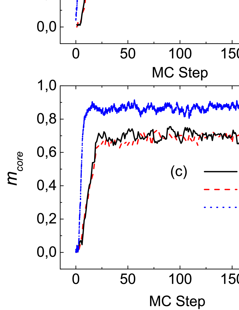
Figure 1: Typical time evolutions of the magnetization $m_{core}$ in Ising model at $T$=2.5 (in unit of $J/k_{B}$) and $h$=0 for (a) $r_{core}$=0.05, (b) $r_{core}$=0.1 and (c) $r_{core}$=0.15, where solid lines, dashed and dotted lines indicated HMCG method, MC simulations and LE approach. Other parameters are $N$=10,000, $\langle k\rangle$=6, $u$=0.01, $p_{c}$=0.6.

MC simulations with Glauber dynamics and LE are performed on the core and the periphery respectively (see methods for the details). Generally, with increasing the temperature $T$, the system undergoes a second-order phase transition at the critical value $T_{c}$ from an ordered state to a disordered one. Figure 1 plots typical time evolutions of the magnetization $m_{core}=\sum\nolimits_{i\in\mathscr{C}}{s_{i}/(r_{core}N)}$ in (1) for different size $r_{core}$ at $T$=2.5 (in unit of $J/k_{B}$) and $h$=0. For both HMCG and the microscopic MC simulations, the systems attain the steady states associated with fluctuating noise after transient time. It is clear that they are in good agreement in the steady-state values of $m_{core}$, as well as their fluctuating amplitudes for both simulations cases at different size $r_{core}$, while the LE is not.

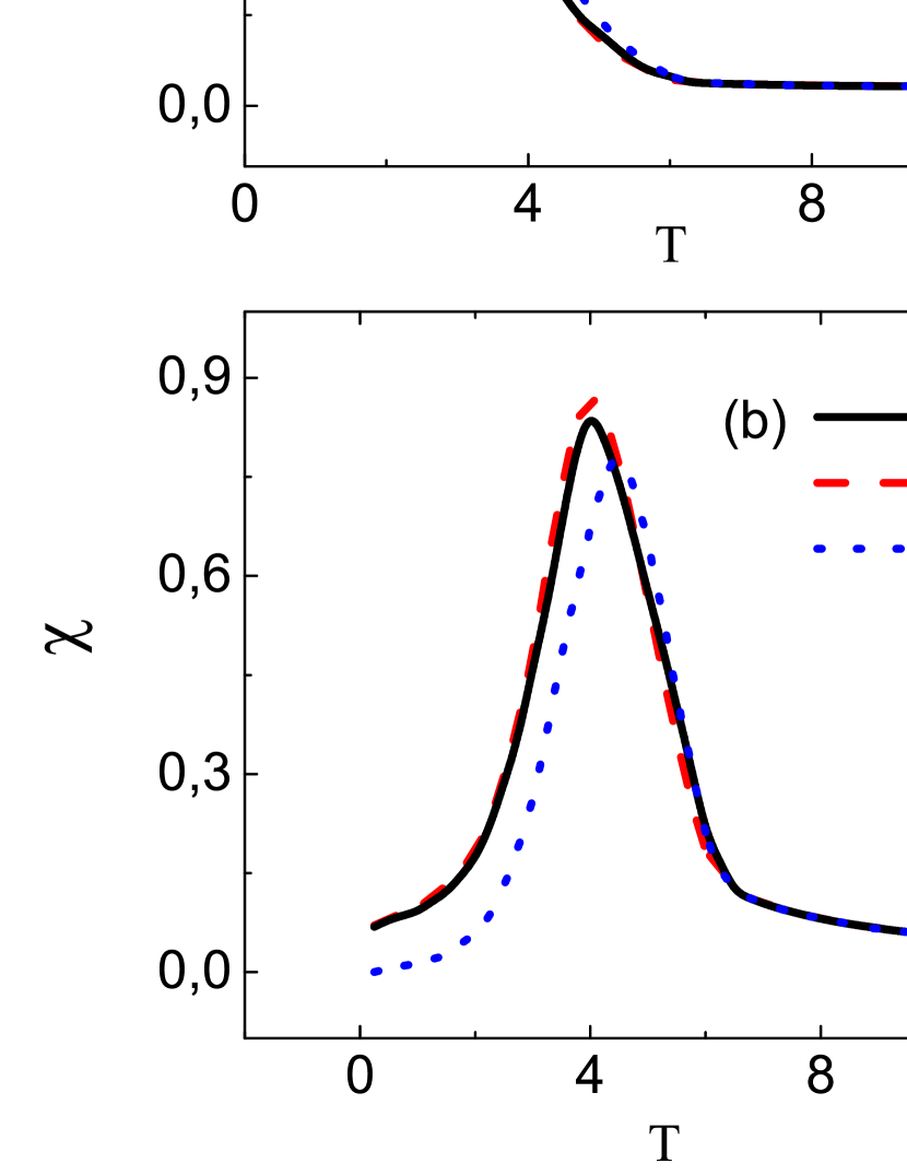
Figure 2: $m_{core}$ and $\chi$ as functions of $T$ for the Ising model on complex networks. The solid lines, dashed and dotted lines correspond to the HMCG, MC and LE simulation results, respectively. Other parameters are the same as in Figure 1.

Furthermore, $m_{core}$ as a function of $T$ is plotted in Figure 2(a), obtained from our HMCG method, micro-MC simulations and LE. Again, the agreements between HMCG and MC are excellent, further demonstrating the validity of HMCG method. In order to ensure that the microscopic configurations are nearly identical between both methods, we calculate the susceptibility $\chi=r_{core}N(\langle m_{core}^{2}\rangle-\langle m_{core}\rangle^{2})/(k_{B}T)$, since $\chi$ is related to the variance of the magnetization according to the fluctuation-dissipation theorem, and compare $\chi$ as a function of $T$ in Figures 2(b). Very good agreement is again seen between HMCG and MC method.

Application to the networked SIS model

Concerning nonequilibrium scenarios, a prototype example is the spreading dynamics of SIS models [29, 30, 31] on complex network as mentioned above, where individuals inside each node run stochastic infection dynamics as follows:

$$S+I\xrightarrow{\lambda}2I,{\kern 10.0pt}I\xrightarrow{\mu}S$$ (2)

The first reaction indicates that each susceptible (S) individual with the state variable $\sigma=0$ becomes infected upon encountering one infected (I) individual with $\sigma=1$ at a rate $\lambda$. The second one reflects that the infected individuals are cured and become again susceptible at a rate $\mu$. For simplicity (yet without loss of generality), we set $\mu=1$. In this model, a significant and general result is that the system undergoes an absorbing-to-active phase transition at a critical value $\lambda_{c}$ with an increasing infectious rate $\lambda$.

Our numerical simulation starts from a random configuration with several nodes being infected. After an initial transient regime, the system will evolve into a steady state with a constant average density of infected nodes. The steady density of infected nodes $\rho$ is computed by averaging over at least 50 different initial configurations and at least 20 different network realizations for a given $\lambda$. Figure 3 compares typical time evolutions $\rho_{core}=\sum\nolimits_{i\in\mathscr{C}}{\sigma_{i}}/(r_{core}N)$ of the density of infected nodes inside the core at $\lambda=0.8$, for the HMCG method, microscopic MC dynamics, and Langevin approach indicated by the solid, dashed and dotted line respectively. Excellent agreement between HMCG and MC is shown.

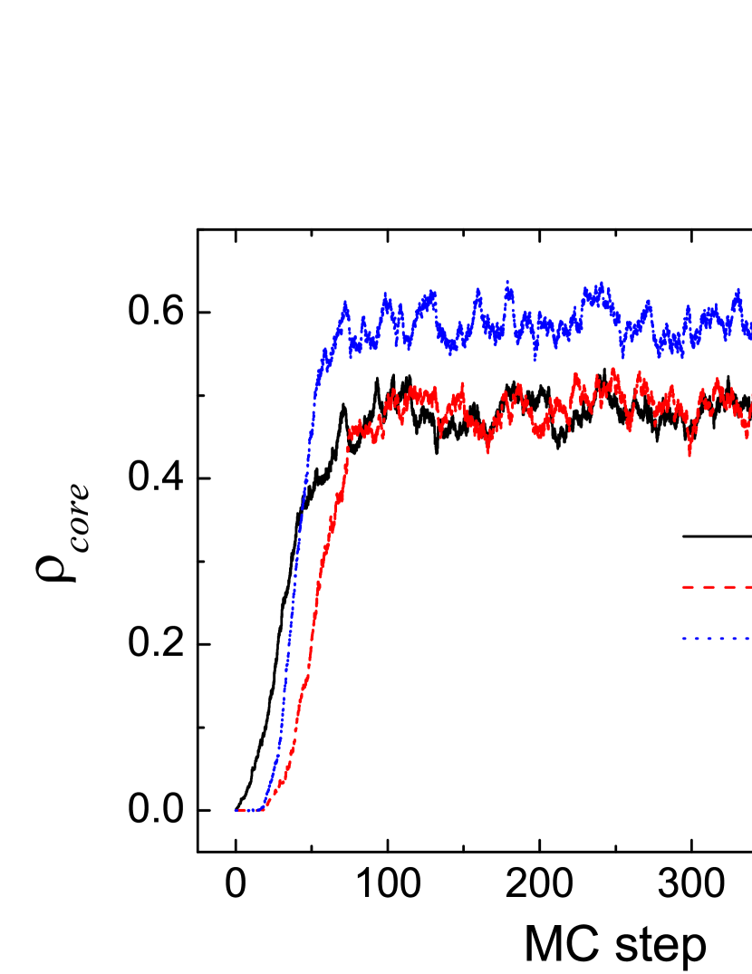
Figure 3: Typical time evolutions $\rho_{core}$ of the density of infected nodes inside the core in SIS model at $\lambda=0.8$ for HMCG method, microscopic MC dynamics, and LE. Other parameters are $N$=10,000, $\langle k\rangle$=6, $r_{core}$=0.1, $u$=0.01, $p_{c}$=0.6.

To further validate the effect of our method, we compare the calculated results of $\rho_{core}$ and normalized susceptibility $\delta=r_{core}N(\langle\rho_{core}^{2}\rangle-\langle\rho_{core}\rangle^{2})/\langle\rho_{core}\rangle$ as a function of $\lambda$ in Figures 4 (a) and (b) respectively, obtained by the HMCG method, the microscopic MC dynamics and LE. Clearly, the agreement between the HMCG and the microscopic MC results remains excellent, while the LE fails. On the one hand, as shown in Fig. 4 (a), the HMCG can reproduce well the main characteristic: the system undergoes a phase transition at a certain threshold rate $\lambda_{c}$, above which $\rho_{core}$ monotonically increases from zero indicating the epidemic spreading, otherwise, i.e., $\lambda<\lambda_{c}$ , the system stays in a healthy state with $\rho_{core}=0$. On the other hand, both HMCG and MC methods exhibit a maximum susceptibility $\delta$ at the threshold $\lambda_{c}$, as can be seen in Fig. 4 (b), which suggests that the microscopic configurations of the HMCG method are nearly identical to those of the original model. Note that the normalized susceptibility $\delta$ adopted here is different from the traditional definition $\delta=r_{core}N(\langle\rho_{core}^{2}\rangle-\langle\rho_{core}\rangle^{2})$[32], because it leads to clearer numerical results, while preserving all the scaling properties of the usual definition [33].

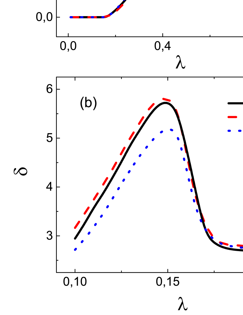
Figure 4: $\rho_{core}$ and $\delta$ as functions of $T$ for SIS model on complex networks. The solid, dashed and dotted lines correspond to the results of HMCG, MC and LE, respectively. Other parameters are same as in Figure 3.

Discussion

Note that the main goal to develop the multiscale coarse grained method is to improve the computational efficiency. We count the CPU time resulted from microscopic MC simulations and from the HMCG method, indicated by $CPU_{MC}$ and $CPU_{HMCG}$ respectively, and compare them in Figures 5 (a) for the Ising model and (b) for the SIS model. It can be seen that, on the one hand, the HMCG method provides substantial computational savings compared to the microscopic MC simulations for the same size of network. On the other hand, the ratio $CPU_{MC}/CPU_{HMCG}$ shows an apparently monotonic dependence on $N$, suggesting that for a given size of the core, the larger the network becomes, the larger computational savings are. One may approximately estimate the total savings by $\frac{{CPU_{MC}}}{{CPU_{HMCG}}}\approx\frac{{N\times\langle k\rangle/2}}{{r_{core}N\times\langle k_{core}\rangle/2+t_{L}}}$, where $\langle k_{core}\rangle=p_{c}(1-u)\langle k\rangle$, denoting the average degree of the group of interest, and $t_{L}$ denotes the computational cost of LE for the rest group. Generally, $t_{L}\ll r_{core}N\times\langle k_{core}\rangle/2$, thus $t_{L}$ can be neglected and $\frac{{CPU_{MC}}}{{CPU_{HMCG}}}\approx\frac{{1}}{{r_{core}\times p_{c}(1-u)}}$ is obtained. Specifically, for $N=10,000$, $\langle k\rangle=6$, $r_{core}=0.1$, $u=0.01$ and $p_{c}=0.6$, we obtain $CPU_{MC}/CPU_{HMCG}\approx 16.8$. Obviously, the computational savings are mainly dependent on the relative size of the interest part compared with that of the entire, and on the density of links of intra-core and inter-parts. Therefore, if the original network is far larger than the part of interest, the efficiency of our method will become more significant.

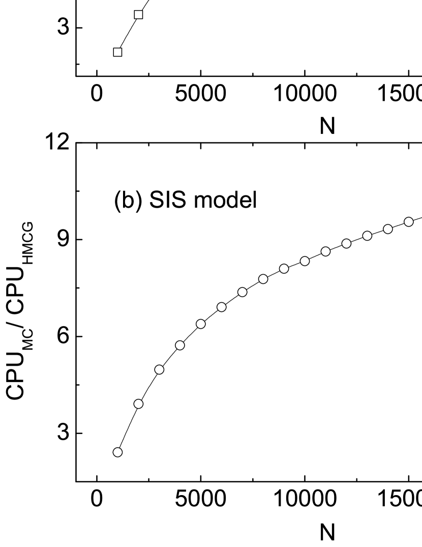
Figure 5: The proportion $CPU_{MC}/CPU_{HMCG}$ as a function of $N$ for the Ising model (a) and for the SIS model (b), where $CPU_{MC}$ and $CPU_{HMCG}$ denote the CPU time resulted from MC and HMCG method respectively. Other parameters in (a) and (b) are same as in Figure 1 and Figure 3 respectively.

In this study, a hybrid multiscale coarse-grained method is proposed that combines a fine simulations for the part of interest with a CG level for the rest of network. Specifically, microscopic MC simulations and LE are employed to treat both parts respectively. Extensively numerical simulations demonstrate that both the networked Ising model and SIS model, two paradigms for equilibrium and nonequilibrium systems, show a very good agreement of the HMCG and MC method. By comparing CPU times for HMCG and MC method, we find that a large computational cost is saved. The HMCG method can not only be suitable to random networks, scale-free networks without or with strength correlation, but also to dense networks and sparse networks [34]. The proposed method thus is general, very easy to implement, and directly related to the microscopics models. Therefore, this method can be applied to a wide variety of networked systems just choosing appropriate microscopic simulation methods, such as kinetic MC method, molecular dynamics, and other CG approaches instead of MC method and LE respectively in view of different real-world scenarios.

Methods

To account for the idea and procedure of the HMCG method, we give a schematic illustration by a module network consisting of five connected random subgraphs with different topologies, as shown in Figure 6. The main idea is as follows: to capture the local information and achieve high efficiency in the simulation, the network is divided into two parts, i.e., the core which is the module of interest and the periphery which consists of the rest ones. Then a fine level simulation and a CG level one are performed on the part of interest and the other part of rest respectively. Here, we adopt a microscopic simulation of detailed allowed by classical MC dynamics and a LE to treat the two parts respectively.

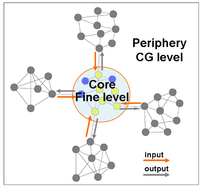
Figure 6: Schematic illustration of the hybrid multiscale coarse-grained method. The original network is divided into two parts, i.e., the part of module of interest named the core, and the part of rest ones named the periphery, which are treated at a fine level and a CG level respectively.

The main steps are summarized below:

(i) Identifying the network parts. According to the requirement of interest, the network is split into two parts, i.e., the core, and the rest one the periphery. We then employ $\mathscr{C}$, $\mathscr{P}$ and $\mathscr{B}$ to denote the adjacency matrices of intra-core, intra-periphery, and inter-parts respectively. Note that $\mathscr{P}$ and $\mathscr{B}$ are coarse grained, while $\mathscr{C}$ preserves so as to to pay close attention to the part of the original system which is different from other CG methods.

(ii) Determining the input and output. In view of the core is the part of interest, we define the flux from the periphery to the core as the input, where the flux is the product of the mean-field of the periphery and the average links between the two parts, and the output is the reverse process.

(iii) Performing simulations. Simulation methods such as MC dynamics, kinetic MC dynamics, molecular dynamics, etc, are performed on the core and the periphery with a more coarse method, e.g., the LE, spectrum coarse graining, $d$-CG, $s$-CG and other CG methods. Specifically, here, MC simulation and LE are employed as the fine level method and the CG method to treat the part of interest and the rest one respectively.

(iv) Improving the method. The CPU time of the HM method and that of microscopic MC simulations are counted and compared as well as the accuracy of the results, and then the method is improved by optimizing the algorithm.

HMCG method for networked Ising model

The MC simulation at the microscopic level follows standard Glauber dynamics: At each step, we randomly selected a node from the group of interest nodes and try to flip its spin with an acceptance probability $1/(1+exp(\Delta E/(k_{B}T)))$, where $\Delta E$ is the associated change of energy due to the flipping process, $k_{B}$ the Boltzmann constant and $T$ the temperature.

A simple recipe of the Glauber algorithm is described as follows:

(1) Choose an initial state

(2) Choose a node $i$ at random, $i\in\mathscr{C}$

(3) Calculate the energy change $\Delta E=\Delta E_{in}+\Delta E_{out}$, resulting from the part of interest and the rest one respectively supposed the spin of node $i$ is flipped. Since $\mathscr{C}$ is known for the part of interest, $\Delta E_{in}$ can be calculated directly by the microscopic simulations, while $\Delta E_{out}$ should be estimated through the mean field coupling between the spin of node $i$ and the net magnetization $m^{\prime}$(to be derived in the next step) of the rest part because that $\mathscr{P}$ is coarse grained

(4) Generate a random number $r$ such that $0<r<1$

(5) If $r<1/(1+exp((\Delta E)/(k_{B}T)))$, flip the spin of node $i$

(6) Go to (2)

Next, we will derive the fluctuation-driven LE for $m^{\prime}$. The average change of magnetization $m^{\prime}$ due to spin-flipping can be written as follows

$$\langle dm^{\prime}\rangle=dm^{\prime}_{\uparrow}\times p_{\uparrow}\times W_{\uparrow,\downarrow}+dm^{\prime}_{\downarrow}\times p_{\downarrow}\times W_{\downarrow,\uparrow}$$ (3)

where $dm^{\prime}_{\uparrow}=-\frac{2}{(1-r_{core})N}$ denotes the net change of magnetization if a up-spin turns to down-spin, and $dm^{\prime}_{\downarrow}=\frac{2}{(1-r_{core})N}$ denotes the reverse process. $p_{\uparrow}=\frac{{1+m^{\prime}}}{2}$ and $p_{\downarrow}=\frac{{1-m^{\prime}}}{2}$ represent the probabilities of up spins and down spins respectively. $W_{\uparrow,\downarrow}$ and $W_{\downarrow,\uparrow}$ represent the transition probabilities from up-spin to down-spin and its reverse process respectively. According to the rule of Glauber dynamics, they take the forms

$$W_{\uparrow,\downarrow} = \frac{1}{{1+e^{\Delta E^{\prime}/T}}}=\frac{1}{2}(1-\tanh(\frac{{\Delta E^{\prime}}}{{2T}}))$$ (4a)

$$W_{\downarrow,\uparrow} = \frac{1}{{1+e^{-\Delta E^{\prime}/T}}}=\frac{1}{2}(1+\tanh(\frac{{\Delta E^{\prime}}}{{2T}}))$$ (4b)

where $\Delta E^{\prime}=2\left({um^{\prime}+\sum\nolimits_{i\in\mathscr{C}}\mathscr{C}s_{i}}\right)/(1-r_{core})N$ is the energy change due to flipping a up-spin within the rest group. Therefore, Eq.(3) can be rewritten as

$$\begin{array}[]{l}\langle dm^{\prime}\rangle=\frac{1}{(1-r_{core})N}(-m^{\prime}+\tanh(\frac{{\Delta E^{\prime}}}{{2T}}))\end{array}$$ (5)

Then, we calculate the mean square deviation of $m^{\prime}$

$$\begin{array}[]{l}\langle dm^{\prime 2}\rangle=\frac{4}{{(1-r_{core})^{2}N^{2}}}\times\frac{{1+m^{\prime}}}{2}\times\frac{1}{2}(1-\tanh(\frac{{\Delta E^{\prime}}}{{2T}}))\\ {\kern 35.0pt}+\frac{4}{{(1-r_{core})^{2}N^{2}}}\times\frac{{1-m^{\prime}}}{2}\times\frac{1}{2}(1+\tanh(\frac{{\Delta E^{\prime}}}{{2T}}))\\ {\kern 30.0pt}=\frac{1}{{(1-r_{core})^{2}N^{2}}}(2-2m^{\prime}\tanh(\frac{{\Delta E^{\prime}}}{{2T}}))\\ \end{array}$$ (6)

When we adopt $dt=1/(1-r_{core})N$, the fluctuation-driven Langevin equation can be obtained

$$\begin{array}[]{l}\frac{{dm^{\prime}}}{{dt}}=-m^{\prime}+\tanh(\frac{{\Delta E^{\prime}}}{{2T}})\\ {\kern 28.0pt}+\sqrt{\frac{1}{{(1-r_{core})N}}(2-2m^{\prime}\tanh(\frac{{\Delta E^{\prime}}}{{2T}}))}\xi(t)\end{array}$$ (7)

where $\xi(t)$ is a Gaussian white-noise satisfying $\langle\xi(t)\rangle=0$ and $\langle\xi(t)\xi(t^{\prime})\rangle=\delta(t-t^{\prime})$.

HMCG method for networked SIS model

To begin, the subgraph of interest is treated with the microscopic MC dynamics as follows

(1) Choose an initial state

(2) Randomly choose a node $i$, $i\in\mathscr{C}$

(3) If $i$ is susceptible, calculate the total number of infected individuals $nI$ of its nearest neighbors, which contains within and without the part of interest, denoted by $nI_{in}$ and $nI_{out}$ respectively. Notice that $nI_{in}=\sum\nolimits_{j\in\mathscr{C}}\mathscr{C}_{ij}\sigma_{j}$ can be calculated directly by the microscopic simulation, while $nI_{out}=\sum\nolimits_{j\in\mathscr{P}}\mathscr{P}_{i,j}\sigma_{j}$ is estimated through the mean field coupling with the average density of infected nodes $\rho^{\prime}$ inside the rest part, since $\mathscr{P}$ is coarse grained. If $i$ is infectious, go to (6)

(4) Generate a random number $r_{1}$ such that $0<r_{1}<1$

(5) If $r_{1}<\lambda nIdt$, $i$ is infected, then go to (2)

(6) Generate a random number $r_{2}$ such that $0<r_{2}<1$

(7) If $r_{2}<dt$, $i$ becomes susceptible, then go to (2)

Then, we will derive the fluctuation-driven LE of $\rho^{\prime}$ for the rest subgraph. Following Ref.[35], one has

$$\begin{array}[]{l}\frac{{d\rho^{\prime}}}{{dt}}=-\rho^{\prime}+\lambda(1-\rho^{\prime})\left({\langle k_{p}\rangle\rho^{\prime}+\sum\nolimits_{i\in\mathscr{C}}\mathscr{C}\sigma_{i}}\right)\\ {\kern 24.0pt}+\sqrt{\frac{1}{{(1-r_{core})N}}[\rho^{\prime}+\lambda(1-\rho^{\prime})(\langle k_{p}\rangle\rho^{\prime}+\sum\nolimits_{i\in\mathscr{C}}\mathscr{C}\sigma_{i})]}\xi(t)\\ \end{array}$$ (8)

where $\langle k_{p}\rangle=(1-u)(1-r_{core}p_{c})\langle k\rangle/(1-r_{core})$ denotes the average degree of the subgraph of the rest, $\sigma_{i}$ is the state variable of node $i$, $\sigma_{i}=0,1$ represent susceptible and infectious respectively. $\xi(t)$ is also a Gaussian white-noise satisfying $\langle\xi(t)\rangle=0$ and $\langle\xi(t)\xi(t^{\prime})\rangle=\delta(t-t^{\prime})$.

Author contributions

C.S. and H.C. conceived the study, constructed the hybrid multiscale coarse-grained method and performed the numerics. C.S., H. C., Z.H. and J.K. discussed the results, drew conclusions, prepared, edited and reviewed the manuscript.

Additional information

Competing financial interests: The authors declare no competing financial interests.

References

- [1] Albert, R. & Barabási, A.-L. Statistical mechanics of complex networks. Rev. Mod. Phys. 74, 47 (2002).
- [2] Dorogovtsev, S. N. & Mendes, J. F. F. Evolution of networks. Adv. Phys. 51, 1079–1139 (2002).
- [3] Boccaletti, S., Latora, V., Moreno, Y., Chavez, M. & Hwang, D.-U. Complex networks: Structure and dynamics. Phys. Rep. 424, 175–308 (2006).
- [4] Arenas, A., Díaz-Guilera, A., Kurths, J., Moreno, Y. & Zhou, C. Synchronization in complex networks. Phys. Rep. 469, 93–153 (2008).
- [5] Dorogovtsev, S. N., Goltsev, A. V. & Mendes, J. F. F. Critical phenomena in complex netwokrs. Rev. Mod. Phys. 80, 1275 (2008).
- [6] Ahn, Y.-Y., Bagrow, J. P. & Lehmann, S. Link communities reveal multiscale complexity in networks. Nature 466, 761–764 (2010).
- [7] Serrano, M. A., Boguná, M. & Vespignani, A. Extracting the multiscale weighted networks. Proc. Natl. Acad. Sci. USA 106, 6483–6488 (2009).
- [8] Jang, H., Na, S. & Eom, K. Multiscale network model for large protein dynamics. J. Chem. Phys. 131, 245106 (2009).
- [9] Balcan, D. et al. Multiscale mobility networks and the spatial spreading of infectious diseases. Proc. Natl. Acad. Sci. USA 106, 21484–21489 (2009).
- [10] Girvan, M. & Newman, M. E. J. Community structure in social and biological networks. Proc. Natl. Acad. Sci. USA 99, 761–764 (2010).
- [11] Boccaletti, S. et al. The structure and dynamics of multilayer networks. Phys. Rep. 544, 1–122 (2014).
- [12] Domenico, M. D., Solé-Ribalta, A., Gómez, S. & Arenas, A. Navigability of interconnected networks under random failures. Proc. Natl. Acad. Sci. USA 111, 8351–8356 (2014).
- [13] Gao, J., Buldyrev, S. V., Stanley, H. E. & Havlin, S. Networks formed from interdependent networks. Nature phys. 8, 40–48 (2012).
- [14] Landau, D. P. & Binder, K. A Guide to Monte Carlo Simulations in Statistcal Physics (Cambridge University Press, Cambridge, 2000).
- [15] Gillespie, D. T. Exact stochastic simulation of coupled chemical reactions. J. Phys. Chem. 81, 2340–2361 (1977).
- [16] Kim, B. J. Geographical coarse graining of complex networks. Phys. Rev. Lett. 93, 168701 (2004).
- [17] Song, C., Havlin, S. & Makse, H. A. Self-similarity of complex networks. Nature 433, 392 (2005).
- [18] Goh, K.-I., G.Salvi, Kahng, B. & Kim, D. Skeleton and fractal scaling in complex networks. Phys. Rev. Lett. 96, 018701 (2006).
- [19] Radicchi, F., Ramasco, J. J., Barrat, A. & S.Fortunato. Complex networks renormalization: Flows and fixed points. Phys. Rev. Lett. 101, 148701 (2008).
- [20] Gfeller, D. & De Los Rios, P. Spectral coarse graining of complex networks. Phys. Rev. Lett. 99, 038701 (2007).
- [21] Gfeller, D. & Rios, P. D. L. Spectral coarse graining and synchronization in oscillator networks. Phys. Rev. Lett. 100, 174104 (2008).
- [22] Kevrekidis, I. G. et al. Equation-free, coarse-grained multiscale computation: Enabling microscopic simulators to perform system-level analysis. Comm. Math. Sci. 1, 715–762 (2003).
- [23] Moon, S. J., Ghanem, R. & Kevrekidis, I. G. Coarse graining the dynamics of coupled oscillators. Phys. Rev. Lett. 96, 144101 (2006).
- [24] Erbana, R., Kevrekidis, I. G., Adalsteinsson, D. & Elston, T. C. Gene regulatory networks: A coarse-grained, equation-free approach to multiscale computation. J. Chem. Phys. 124, 084106 (2006).
- [25] Gross, T. & Kevrekidis, I. G. Robust oscillations in sis epidemics on adaptive networks: Coarse graining by automated moment closure. EPL 82, 38004 (2008).
- [26] Chen, H. S., Hou, Z. H., Xin, H. W. & Yan, Y. J. Statistically consistent coarse-grained simulations for critical phenomena in complex networks. Phys. Rev. E 82, 011107 (2010).
- [27] Shen, C. S., Chen, H. S., Hou, Z. H. & Xin, H. W. Coarse-grained monte carlo simulations of the phase transition of the potts model on weighted networks. Phys. Rev. E 83, 066109 (2011).
- [28] Rabinovich, M. I., Varona, P., Selverston, A. I. & Abarbanel, H. D. I. Dynamical principles in neuroscience. Rev. Mod. Phys. 78, 1213–1264 (2006).
- [29] Anderson, R. & R.M.May. Infectious Diseases in Humans (Oxford University Press, Oxford, 1992).
- [30] Daley, D. J. & Gani, J. Epidemic Modelling (Cambridge University Press, Cambridge, 1999).
- [31] Pastor-Satorras, R., Castellano, C., Van Mieghem, P. & Vespignani, A. Epidemic processes in complex networks. Rev. Mod. Phys. 87, 925–979 (2015).
- [32] Marro, J. & Dickman, R. Nonequilibrium Phase Transitions in Lattice Models (Cambridge University Press, Cambridge, 1999).
- [33] Ferreira, S. C., Castellano, C. & Pastor-Satorras, R. Epidemic thresholds of the susceptible-infected-susceptible model on networks: A comparison of numerical and theoretical results. Phys. Rev. E 86, 041125 (2012).
- [34] Karrer, B., Newman, M. E. J. & Zdeborová, L. Percolation on sparse networks. Phys. Rev. Lett. 113, 208702 (2014).
- [35] Boguñá, M., Castellano, C. & Pastor-Satorras, R. Langevin approach for the dynamics of the contact process on annealed scale-free networks. Phys. Rev. E 79, 036110 (2009).
Acknowledgements
This work was supported by the National Basic Research Program of China (2013CB834606) and by the National Natural Science Foundation of China (Grants No. 11475003, 11205002 and No. 21473165). C.S. was also funded by the China Scholarship Council (CSC) and Natural Science Foundation of Anhui Province (Grant No.1408085MA09).