Probing the Heavy Neutrinos of Inverse Seesaw Model at the LHeC

Abstract

We consider the production of a heavy neutrino and its possible signals at the Large Hadron-electron Collider (LHeC) in the context of an inverse-seesaw model for neutrino mass generation. The inverse seesaw model extends the Standard Model (SM) particle content by adding two neutral singlet fermions for each lepton generation. It is a well motivated model in the context of generating non-zero neutrino masses and mixings. The proposed future LHeC machine presents us with a particularly interesting possibility to probe such extensions of the SM with new leptons due to the presence of an electron beam in the initial state. We show that the LHeC will be able to probe an inverse scenario with much better efficacy compared to the LHC with very nominal integrated luminosities as well as exploit the advantage of having the electron beam polarized to enhance the heavy neutrino production rates.

I Introduction

The discovery of the Higgs boson Higgs:lhc has been a remarkable achievement by the experiments running at the Large Hadron Collider (LHC), which in a profound way give closure to the predictions within the Standard Model (SM) picture of particle physics. However, some unanswered questions remain which forces us to look beyond the SM (BSM). One of the intriguing issues that needs immediate attention is the existence of tiny non-zero neutrino masses. Neutrino oscillation data reveals that at least two of the three light neutrinos of the SM are massive and also indicates a significant mixing among all the three neutrino states (for a review, see e.g, neut:osc ). SM, devoid of any right-handed neutrinos, fails to account for this particular phenomenological aspect. The simplemost natural extension of the SM comes in the form of type-I seesaw mechanism csaw which adds one additional heavy Majorana neutrino to the SM particle content. As a consequence of mixing with this heavy neutrino state, one of the light neutrino gets a non-zero mass at the tree level. Another neutrino gains non-zero mass at one loop level, reproducing the neutrino oscillation data perfectly. However, the smallness of the neutrino masses ensure that either the left-right Yukawa coupling is very small, $\sim 10^{-6}$ or the heavy Majorana neutrino mass is extremely heavy, $\sim 10^{16}$ GeV, making the new features of this model virtually untestable at the present collider experiments.

Inverse Seesaw Mohapatra:1986aw ; Nandi:1985uh ; Mohapatra:1986bd is a well motivated BSM scenario from the viewpoint of neutrino mass generation. Owing to the presence of a very small lepton number violating parameter, $\mu_{S}\sim$ eV which is responsible for the smallness of the light neutrino masses in the model, the Yukawa coupling generating the Dirac neutrino mass term can be quite large ($\sim$ 0.1) even in the presence of sub TeV heavy neutrino masses in this scenario. This leads to a plethora of phenomenological implications in non-supersymmetric Das:2012ze ; Bandyopadhyay:2012px ; Dev:2013wba ; Das:2014jxa ; Arganda:2014dta ; Deppisch:2015qwa ; Arganda:2015naa ; Arganda:2015ija ; Das:2015toa as well as in supersymmetric context Hirsch:2009ra ; Mondal:2012jv ; BhupalDev:2012ru ; DeRomeri:2012qd ; Banerjee:2013fga . Two obvious aspects of any neutrino mass model which can then be probed at the collider experiments are, production of the additional heavy neutrino states and studying the effects of left-right neutrino mixing. As the Yukawa couplings are large in the inverse seesaw model, it is possible to obtain flavour specific leptonic final states through their production and subsequent decays. Search for such heavy neutrinos in this kind of models, at LHC has been discussed in detail Datta:1993nm ; Han:2006ip ; delAguila:2007qnc ; Huitu:2008gf ; Atre:2009rg ; Das:2012ze ; Dev:2013wba ; Das:2014jxa ; Chen:2011hc ; Alva:2014gxa ; Deppisch:2015qwa ; Das:2015toa . Electron enriched final states are usually suppressed in the usual models of neutrino mass generation due to the stringent constraints derived from the non-observation of neutrinoless double beta decay ($0\nu\beta\beta$) Deppisch:2015qwa on the heavy neutrino mixing with $\nu_{e}$. In the inverse seesaw mechanism, however, this constraint is relaxed due to the extremely small mass splitting between the heavy neutrinos with opposite CP-properties, forming a quasi-Dirac state owing to a ${\mathcal{O}}(eV)$ lepton number violating (LNV) parameter, $\mu_{S}$. As a matter of fact, the smallness of $\mu_{S}$ forces all the LNV processes to be suppressed in such scenarios. Therefore, the usual smoking gun LNV signals of heavy Majorana neutrino are not ideal to look for in inverse seesaw model. However, a loose $0\nu\beta\beta$ constraint opens the additional possibility for an electron enriched final state. Heavy neutrino production associated with an electron has been studied at the LHC in the context of an inverse seesaw model Das:2012ze . It was observed that one expects 5$\sigma$ statistical significance over the SM backgrounds for a trilepton signal at the 14 TeV run of LHC with 11 ${\rm fb}^{-1}$ integrated luminosity and degenerate heavy neutrino masses of 100 GeV. It turns out that the trilepton signal is by far the best channel to probe the inverse seesaw model at the LHC. However, if the heavy neutrino states are much more massive, then these heavier states will be produced with much reduced rates which in turn affects the sensitivity of probing these heavy states at the LHC. An alternative search strategy for much heavier states can, in fact be carried out more efficiently at a different scattering experiment such as the proposed Large Hadron-Electron Collider (LHeC) AbelleiraFernandez:2012cc ; Bruening:2013bga which is the main thrust of this work. To highlight this, we study the heavy neutrino production in the inverse seesaw model at LHeC and determine its signal strengths through various leptonic channels.

LHeC would be the next high energy $e-p$ collider after HERA, supposed to be built at the LHC tunnel. The design is planned so as to collide an electron beam with a typical energy range, 60-150 GeV with a 7 TeV proton beam producing center of mass energy close to 1.3 TeV at the parton level. It is expected to achieve 100 ${\rm fb}^{-1}$ integrated luminosity per year. Lepton number violating heavy Majorana neutrino signals and other phenomenological consequences have already been explored in the context of the $e-p$ colliders Ingelman:1993ve ; Liang:2010gm ; Blaksley:2011ey ; Duarte:2014zea ; Mondal:2015zba ; Lindner:2016lxq and future lepton colliders Basso:2013jka ; Antusch:2014woa ; Antusch:2015mia . Note however that LHeC has a distinct advantage over the LHC for this kind of searches since the electron in the initial state can be polarised. This very interesting and important aspect of using the polarisation of the initial electron beam to study specific BSM scenarios at LHeC was first pointed out by us in Ref.Mondal:2015zba . A dominantly polarised (left/right) electron beam could thereby enhance a new physics signal for specific production channels while also affecting the corresponding SM background, making it an additional tool to explore BSM physics as was envisaged for linear electron-positron colliders. Although for a high energy ($\sim 100$ GeV) electron beam it is difficult to maintain a high enough polarisation, for a 60 GeV beam, polarisation of upto 80$\%$ can be achieved AbelleiraFernandez:2012cc . Such a machine will therefore help determine quite distinctly the nature of specific production modes of the heavy neutrinos Mondal:2015zba .

II The Model

The SM particle content is extended by the addition of two fermion singlets to each generation. These two singlets, $N^{c}$ and $S$ are assigned lepton numbers -1 and +1 respectively. The extended Lagrangian looks like:

$${\cal L}=\epsilon_{ab}y_{\nu}^{ij}L^{a}_{i}H^{b}N^{c}_{j}+{M_{R}}^{ij}N^{c}_{i}S_{j}+{\mu_{S}}^{ij}S_{i}S_{j},$$ (1)

where $\mu_{S}$ is a small ($\sim{\rm eV}$) lepton number violating ($\Delta L=2$) parameter. The $9\times 9$ neutrino mass matrix in the basis $\{\nu_{L},N^{c},S\}$ looks like:

$${\cal M}_{\nu}=\left(\begin{array}[]{ccc}{\bf 0}&M_{D}&{\bf 0}\\ M_{D}^{T}&{\bf 0}&M_{R}\\ {\bf 0}&M_{R}^{T}&\mu_{S}\end{array}\right),$$ (5)

where, $M_{D}=y_{\nu}\,v$ is the Dirac neutrino mass matrix, $v\simeq 174$ GeV being the vacuum expectation value (vev) of the Higgs field in the SM. Under the approximation, $\|\mu_{S}\|\ll\|M_{R}\|$ (where $\|M\|\equiv\sqrt{{\rm Tr}(M^{\dagger}M)}$), one can extract the $3\times 3$ light neutrino mass matrix. Upto leading order in $\mu_{S}$ it looks like:

$$M_{\nu}=\left[M_{D}M_{R}^{T^{-1}}\right]\mu_{S}\left[(M_{R}^{-1})M_{D}^{T}\right]\equiv F\mu_{S}F^{T},$$ (6)

where $F=M_{D}M_{R}^{T^{-1}}$. It is evident from Eq. (6), that the smallness of neutrino mass here depends on the smallness of the lepton-number violating parameter $\mu_{S}$ instead of the smallness of $M_{D}$ and/or heaviness of $M_{R}$ as in the canonical type-I seesaw case. Consequently, one can have a $M_{R}$ below the ${\rm TeV}$ range even with a comparatively large Dirac Yukawa coupling, ($y_{\nu}\sim 0.1$). Both $M_{D}$ and $M_{R}$ can be kept strictly diagonal and the neutrino oscillation data can be fit by an off-diagonal $\mu_{S}$, where,

$$\mu_{S}=F^{-1}M_{\nu}{F^{T}}^{-1}$$ (7)

$M_{\nu}$ can easily be constructed from the neutrino oscillation parameters :

$$M_{\nu}=U_{PMNS}M_{\nu}^{\rm diag.}U^{T}_{PMNS},$$ (8)

where, $M_{\nu}^{\rm diag.}$ is the diagonal neutrino mass matrix and $U_{PMNS}$ is the diagonalising unitary Pontecorvo-Maki-Nakagawa-Sakata (PMNS) matrix. In order to construct the $U_{PMNS}$ and $M_{\nu}^{\rm diag.}$ matrices, We have considered the most updated neutrino oscillation parameters Gonzalez-Garcia:2015qrr obtained from global fit of the experimental data. The oscillation parameters for normal hierarchy in neutrino masses as well as the resulting PMNS matrix we used are presented in Table 1.

Parameters	Values
${\rm sin}^{2}\theta_{12}$	$0.304^{+0.013}_{-0.012}$
${\rm sin}^{2}\theta_{23}$	$0.452^{+0.052}_{-0.028}$
${\rm sin}^{2}\theta_{13}$	$0.0218^{+0.001}_{-0.001}$
$\Delta m^{2}_{21}~{}{\rm eV}^{2}$	$(7.50^{+0.19}_{-0.17})\times 10^{-5}$
$\Delta m^{2}_{32}~{}{\rm eV}^{2}$	$(2.457^{+0.047}_{-0.047})\times 10^{-3}$
$U_{PMNS}$	$\left(\begin{array}[]{ccc}0.825&0.545&0.148\\ -0.491&0.563&0.665\\ 0.280&-0.621&0.732\\ \end{array}\right)$

Table 1: Three flavor neutrino oscillation data obtained from global fit for normal hierarchy in neutrino masses as presented in Ref. Gonzalez-Garcia:2015qrr and the resulting PMNS matrix.

Once we have $M_{\nu}$ in the form of Eq. 8, it can be plugged back into Eq. 7 to find the $\mu_{S}$ matrix.

III Heavy neutrino signals

Same sign dilepton signature has been studied extensively in order to probe the possible Majorana nature of heavy neutrinos and their mixing with the light SM-like neutrinos. At the LHC, the usual channel that is considered is $pp\rightarrow W^{\pm}\rightarrow\ell^{\pm}N$, where $N$ subsequently decays into a lepton associated with on-shell or off-shell $W$ which then decays hadronically. For Majorana neutrinos, this results in the same-sign dilepton final state ($\ell^{\pm}\ell^{\pm}jj$) with negligible missing energy. However, cross-section for this final state is rendered small either by the constrained Yukawa coupling or heavy Majorana neutrino masses. Most stringent constraint on these parameters in case of usual neutrino mass models, e.g. type-I seesaw extended SM, is derived from the non-observation of neutrinoless double beta decay ($0\nu\beta\beta$); $\sum_{N}\frac{V_{eN}}{m_{N}}<5\times 10^{-8}~{}{\rm GeV}^{-1}$ Deppisch:2015qwa . Thus, heavy Majorana neutrinos which couple to the electron are usually neglected at collider experiments . However, in the case of inverse seesaw extended SM, the contribution to $0\nu\beta\beta$ is extremely small due to the presence of a small $\mu_{S}$ as already mentioned. Hence this particular constraint becomes non-restrictive for electron channels Das:2012ze . Therefore it becomes an imperative channel to probe an inverse seesaw scenario at a machine like LHeC where the electron-type heavy neutrino can be directly produced. Non-observation of any Majorana neutrino signal at the LHC so far from di-muon final state translates into a bound on the light-heavy neutrino mixing parameter, $|V_{\mu N}|^{2}\sim 10^{-2}-10^{-1}$ for heavy neutrino masses $m_{N}$=100-300 GeV ATLAS:2012ak ; ATLAS:2012yoa ; Chatrchyan:2012fla .

The special feature of an inverse seesaw extended SM is that it can simultaneously have a $\sim$ 100 GeV heavy Majorana neutrino with $\sim$ 0.1 Yukawa coupling even after satisfying neutrino oscillation data. This makes it particularly interesting phenomenologically. In this article, we look into the various possible final states in this framework in the context of LHeC. The fact that the LHeC can produce an electron beam that can be highly polarised upto a certain energy, makes it even more interesting phenomenologically to probe such scenarios. Since the SM singlet neutrino only mixes with the left-handed leptons, a dominantly left-polarised electron beam in the initial state is expected to increase the cross-section significantly. Additionally, being an $e-p$ collider, LHeC will produce much cleaner signals compared to the LHC.

III.1 Analysis

Here we intend to look into the possible production modes of the heavy neutrino. The dominant contribution comes from the channel $e\,p\to N\,j$ while another (sub-dominant) contributing process can be identified as $e\,p\to N\,j\,W^{-}$, where $N$ indicates the heavy right-handed neutrino states. An inclusive contribution to the signal also comes from a heavy neutrino mediated process given by $e\,p\to e^{-}\,j\,W^{-}$. This may result into final states consisting of different lepton-jet multiplicity and missing energy.

In Fig. 1 we show the $Nj$ production channel and subsequent decays of $N$ to give rise to the following possible final states (at parton-level):

• $e^{+}$/$e^{-}$ + n-jets ($n=3$)

• $e^{\pm}\ell^{\mp}$ + n-jets ($n=1$) + ${E\!\!\!\!/_{T}}$.

Here, $\ell$ represents either an electron or muon in the final state.

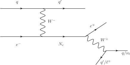
Figure 1: Feynman diagram for the various final states derived from $Nj$ production channel.

This clearly gives the most dominant contribution to the signal for a heavy neutrino production. However, a higher jet- and lepton-multiplicity signal also can arise from another production mode for $N$, which is usually neglected but can in principle also contribute to the signal rates arising from $Nj$ production. This is shown in Fig. 2, where the $NjW^{-}$ production channel and subsequent decays of $N$ and $W^{-}$, give rise to the following possible final states (at parton-level):

• $e^{+}$/$e^{-}$ + n-jets ($n=5$)

• $e^{\mp}\ell^{-}$ + n-jets ($n=3$) + ${E\!\!\!\!/_{T}}$

• $e^{\mp}\ell^{\pm}\ell^{-}$ + n-jets ($n=1$) + ${E\!\!\!\!/_{T}}$.

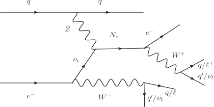
Figure 2: Feynman diagram for the various final states derived from $NjW^{-}$ production channel.

As one can see that all the channels listed for the $NjW^{-}$ mode can in principle contribute to the final states arising from the $Nj$ production mode, where the higher multiplicity in jets or leptons can be reduced through mismeasurements, trigger efficiencies, etc. Finally, an $N$ mediated channel ($e^{-}jW^{-}$), which is at the same order in coupling as the $NjW^{-}$ process, may also contribute to the signal which we therefore include in our analysis. This subprocess is shown in Fig. 3 and gives rise to the following possible final states (at parton-level) which is exactly the same as $Nj$ production:

• $e^{\pm}$ + n-jets ($n=3$)

• $e^{\pm}\ell^{-}$ + n-jets ($n=1$) + ${E\!\!\!\!/_{T}}$.

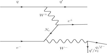
Figure 3: Feynman diagram for the various final states derived from $e^{-}jW^{-}$ production channel.

Note that, although we show all the possible final states arising from the above three production channels, including the lepton number violating processes which have extremely small cross-sections within the framework of inverse seesaw model, as already mentioned. Hence among all the above listed final states we shall ignore the LNV contributions and only concentrate on the lepton number conserving ones, which arise in the inverse seesaw scenario.

We now discuss the production rates in the different channels both in the context of LHC and LHeC. While calculating the cross-sections at LHC, we chose the center of mass energy of 14 TeV which would give the largest rate for LHC. Note that, at the LHC, both $pp\to Nj$ and $pp\to NjW^{-}$ production channels will be absent since both of them are lepton number violating processes ($\Delta L=1$), whereas models for Majorana neutrinos allow only $\Delta L=2$ violations. Therefore the dominant production channel at LHC for the heavy neutrino is $pp\rightarrow W^{\pm}\rightarrow\ell^{\pm}N$. For LHeC, we have considered a 60-GeV electron beam colliding with a 7 TeV proton beam. We compute the cross-section with both polarised and unpolarised electron beams to assess how much the cross-section may actually differ. We calculate the cross section for the different production modes of the heavy neutrino as a function of its mass, shown in Fig. 4. We have parametrized the heavy-light neutrino mixing term as a function of the heavy neutrino mass, using the condition $V_{eN}=y_{\nu}^{11}\,v/m_{N}$ where we have fixed $y_{\nu}^{11}=0.1$. Note that this gives a substantially conservative estimate of the mixing for heavier masses, as the limits for such mixing is expected to be weaker as the mass $m_{N}$ increases.

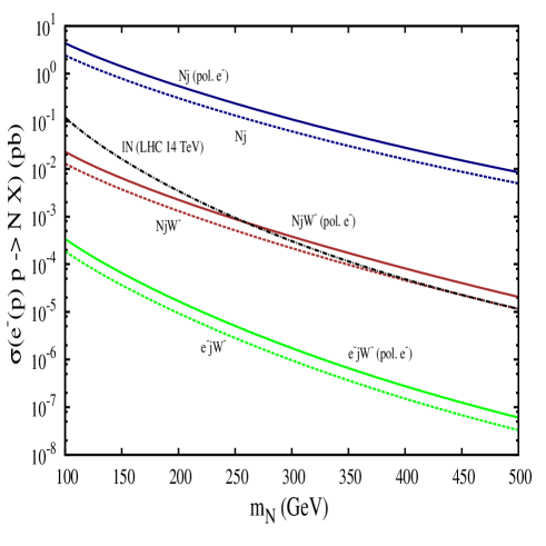
Figure 4: Production cross-section of $Nj$, $NjW^{-}$ and $e^{-}jW^{-}$ at LHeC with and without 80% left-polarised electron beam along with that of the most dominant production mode of the heavy neutrinos at the LHC, $\ell N$, with varying heavy neutrino masses. The blue solid and dotted lines represent the variation of production cross-section in $Nj$ channel with and without the left-polarised electron beam. Likewise, the brown and the green lines represent the $NjW^{-}$ and $e^{-}jW^{-}$ production channels respectively. The black (dashed) line corresponds to the $\ell N$ production cross-section at the LHC at 14 TeV center of mass energy.

Fig. 4 shows the variation of the cross-section of the aforementioned production channels at LHeC. As a comparison to what LHC may achieve in terms of production rates for such a heavy neutrino, we also show the variation of the cross-section, $\sigma(pp\to\ell N)$ which is the most dominant production channel of the heavy neutrino at the LHC . The blue, brown and green dotted lines correspond to the cross-sections at LHeC with an unpolarised electron beam for $Nj$, $NjW^{-}$ and $e^{-}jW^{-}$ production modes respectively. The corresponding solid lines of same colour show the relative enhancement in the cross-sections when the electron beam is dominantly left-polarised (80%). As one can see, the rates improve by almost a factor of 2 over the entire range of the heavy neutrino mass in case of a polarised $e^{-}$ beam. The cross-section for $\ell N$ production at the 14 TeV run of LHC, shown in black (dashed) line in Fig. 4, is quite small when compared to the $Nj$ production mode at LHeC. It however does compete in the low $m_{N}$ region with the LHeC production rates of the significantly sub-dominant $NjW^{-}$ production. Interestingly, for heavier masses, LHeC with a polarised electron beam provides a better rate even in this mode. Note that the $e^{-}jW^{-}$ channel which was included is unlikely to be of any significance due to its extremely small cross-section. The large suppression, when compared to the $NjW^{-}$ production can be understood from the fact that the proton radiates a $W^{-}$ in the t-channel for $e^{-}jW^{-}$ while a $Z$ boson mediates the $NjW^{-}$. This implies that while the valence $u$ and $d$ quarks of the proton contribute to the $NjW^{-}$ production, $e^{-}jW^{-}$ production is only through the valence $d$ quark. Thus, we can safely ignore this production channel for the rest of our analysis.

We choose to carry out our analysis for two particular benchmark points to probe one of the several heavy neutrinos in the model. It is evident from the neutrino mass matrix in Eq. 5 that $\mu_{S}$ being a very small parameter, the masses of the heavy neutrino states are dictated by the choice of the matrix $M_{R}$. Among the six heavy neutrino states, there exist three mass degenerate pairs. We chose to keep the lightest of these heavy neutrino pairs at sub-TeV mass and make the rest of them very heavy. For example, we chose ${M_{R}}^{11}\simeq m_{N}$=150 GeV while fixing ${M_{R}}^{22}$=${M_{R}}^{33}$=1000 GeV. For simplicity, a diagonal structure for both $M_{R}$ and $y_{\nu}$ is assumed. As a consequence, the $m_{N}=150$ GeV heavy neutrino states will only couple to the electron. Accordingly we have fit the neutrino oscillation data with an off-diagonal $\mu_{S}$ which we found can easily accommodate all experimental results of the neutrino sector. Similarly, another benchmark is set with $m_{N}=400$ GeV. For our collider analysis, we keep the mixing $V_{eN}$ for this benchmark to be the same as that for $m_{N}=150$ GeV. Table 2 shows our choices of the neutrino sector parameters in order to fit the neutrino oscillation data.

Parameters	BP1	BP2
$M_{R}$ (GeV)	(150.0,1000.0,1000.0)	(400.0,1000.0,1000.0)
$y_{\nu}$	(0.1,0.01,0.01)	(0.1,0.01,0.01)
$\mu_{S}$ (keV)	$\left(\begin{array}[]{ccc}0.0003&0.0380&0.0126\\ 0.0380&8.3424&7.1666\\ 0.0126&7.1666&10.1186\\ \end{array}\right)$	$\left(\begin{array}[]{ccc}0.0020&0.1014&0.0335\\ 0.1014&8.3424&7.1666\\ 0.0335&7.1666&10.1186\\ \end{array}\right)$

Table 2: Choices of the neutrino sector input parameters $M_{R}$ and $y_{\nu}$ and the resulting $\mu_{S}$ matrix from neutrino oscillation data for our two benchmark points. Note that, in order to fit the neutrino oscillation data, we consider the experimental constraints assuming only normal hierarchy among the neutrino masses. The corresponding experimental constraints are taken from Ref. Gonzalez-Garcia:2015qrr .

With these choices of the parameters, we now proceed to study the signal arising from the production channels $NjW$ and $Nj$.

The complete model has been implemented in SARAH (v4.6.0) sarah . The mass spectrum for the inverse seesaw model has been subsequently generated using SPheno (v3.3.6) spheno along with the mixing matrices and decay strengths. We have used MadGraph5@aMCNLO (v2.3.3) mad5 to generate parton level events for the signal and backgrounds. Subsequent decay, showering and hadronisation are done using PYTHIA (v6.4.28) pythia6 whereas a proper MLM matching procedure has been employed for the multi-jet final states.

To analyse the signal and background events we use the following set of selection criteria to isolate the leptons and jets in the final state:

• Electrons and muons in the final state should have $p_{T}^{\ell}>20$ GeV,$|\eta^{e}|<2.5$ and $|\eta^{\mu}|<2.5$.

• Photons are counted if $p_{T}^{\gamma}>10$ GeV and $|\eta^{\gamma}|<2.5$ as the leptons.

• Leptons should be separated by, $\Delta R_{\ell\ell}>0.2$.

• Leptons and photons should be separated by, $\Delta R_{\ell\gamma}>0.2$.

• For the jets we require $p_{T}^{j}>40$ GeV and $|\eta^{j}|<2.5$.

• Jets should be separated by, $\Delta R_{jj}>0.5$.

• Leptons and jets should be separated by, $\Delta R_{\ell j}>0.4$.

• Hadronic energy deposition around an isolated lepton must be limited to $\sum p_{T_{hadron}}<0.2\times p_{T}^{\ell}$.

As already mentioned, because of the choice of digonal $M_{R}$ and $y_{\nu}$, the $N$ always decays into an $e$ or $\nu_{e}$ associated final state. Here we only consider $N$ decaying into an electron and $W$. Hence all the possible final states consist of an electron accompanied by other leptons and jets. Although the lepton number violating final state $e^{+}$ + n-jets derived from both $NjW$ and $Nj$ production channels have practically negligible SM background their signal cross-section is also highly suppressed due to the small lepton number violating parameter. Hence LNV final states are not ideal to probe inverse seesaw scenario. Instead, we concentrate only on the lepton number conserving final states arising from both the production channels. Apart from the cascade, some additional jets are expected to appear from the initial and (or) final state radiation while showering. Hence we chose various final states consisting of a minimum number of jets that we expect to come from the cascades itself, depending upon the leptonic or hadronic decays of the $W$-boson.

The SM background events were generated for all the subprocesses that contribute towards the different final states that we consider for the signal. We have explicitly chosen to compute the continuum SM background where the dominant contributions arise mostly from the gauge boson mediated $t$-channel processes. After selecting both the signal and background events through the aforementioned selection criteria, we further put a minimal ${E\!\!\!\!/_{T}}$ requirement of 20 GeV on all final states under consideration.

III.2 Results

In this section, we present the results of our simulation at two different heavy neutrino masses, $m_{N}=150$ GeV and 400 GeV. For the $m_{N}=150$ GeV case, we apply the aforementioned cuts whereas for the heavier neutrino mass scenario we impose slightly harder cuts to reduce SM backgrounds more effectively. Note that for the signal, the electron coming from the decay of the heavy neutrino would carry a $p_{T}$ depending on the mass difference $\Delta M=m_{N}-M_{W}$. Thus for a much heavier neutrino such as $m_{N}=400$ GeV, a stronger $p_{T}$ requirement on the leading $e^{-}$ would help. This is also evident from Fig. 5, which shows the above mentioned feature for our two different mass choices of $N$.

Figure 5: Transverse momentum of the $e^{-}$ originating from decaying $N_{e}$ for $m_{N}=150$ GeV and 400 GeV obtained from the $Nj$ production channel.

We therefore demand that the leading electron must have a $p_{T}>100$ GeV for the $m_{N}=400$ GeV signal. We keep the rest of the selection criterion same as for the $m_{N}=150$ GeV. We present in Table 3, the resulting cross-section for all the signal channels and also for the corresponding SM backgrounds whereas in Table 4, we show the required integrated luminosity to achieve a $3\sigma$ excess in the four final states we have studied at the LHeC. Note that as the $NjW^{-}$ production cross-section becomes negligibly small for $m_{N}=400$ GeV, we only present the final state contributions for this benchmark, arising from the $Nj$ production mode.

$m_{N}$	Final States	$\sigma$ (fb)	$\sigma$ (fb)	$\sigma$ (fb)
(GeV)		(NjW)	(Nj)	(SM)
150	$e^{-}$ + n-jets ($n\geq 3$) + ${E\!\!\!\!/_{T}}$	0.36	12.86	38.05
	$e^{-}\ell^{-}$ + n-jets ($n\geq 3$) + ${E\!\!\!\!/_{T}}$	0.02	-	0.01
	$e^{-}\ell^{+}$ + n-jets ($n\geq 1$) + ${E\!\!\!\!/_{T}}$	0.68	87.68	24.45
	$e^{-}\ell^{+}_{i}\ell^{-}_{j}$ + n-jets ($n\geq 1$) + ${E\!\!\!\!/_{T}}$	0.04	-	0.72
400	$e^{-}$ + n-jets ($n\geq 3$) + ${E\!\!\!\!/_{T}}$	-	1.42	15.21
	$e^{-}\ell^{+}$ + n-jets ($n\geq 1$) + ${E\!\!\!\!/_{T}}$	-	2.20	6.30

Table 3: Signal cross-sections for various final states obtained from $NjW$ and $Nj$ productions computed for two different heavy neutrino masses. The last column represents corresponding background cross-sections as obtained from the SM. Note that, the quoted cross-sections are obtained for different sets of cuts at the two different heavy neutrino masses.

We calculate the statistical significance for the signal using

$${\mathcal{S}}=\sqrt{2\times\left[(s+b){\rm ln}(1+\frac{s}{b})-s\right]},$$ (9)

where, $s$ and $b$ represent the signal and background event counts respectively, by combining the event rates of both the production channels $Nj$ and $NjW^{-}$.

	Required luminosity ($\mathcal{L}$)
	for ${\mathcal{S}}=3{\sigma}$ (in $fb^{-1}$)
Final States	$m_{N}$ (in GeV)
	$150$	$400$
$e^{-}$ + n-jets ($n\geq 3$) + ${E\!\!\!\!/_{T}}$	2.2	$70.0$
$e^{-}\ell^{-}$ + n-jets ($n\geq 3$) + ${E\!\!\!\!/_{T}}$	347.3	-
$e^{-}\ell^{+}$ + n-jets ($n\geq 1$) + ${E\!\!\!\!/_{T}}$	0.05	13.0
$e^{-}\ell^{+}_{i}\ell^{-}_{j}$ + n-jets ($n\geq 1$) + ${E\!\!\!\!/_{T}}$	$4.12\times 10^{3}$	-

Table 4: An estimate of the required integrated luminosity to achieve a $3\sigma$ statistical significance for each of the four final states for two different heavy neutrino masses at LHeC.

All the final states are associated with at least one $e^{-}$ originating from the $N$ decay, irrespective of how the $W$’s have decayed. The rate of the final state $e^{-}$ + n-jets ($n\geq 3$), arising from $NjW^{-}$ production is rather small due to the small production cross-section, but non-vanishing for the $m_{N}=150$ GeV signal. For the heavier neutrino mass region, this contribution can be easily neglected. However, the combined rate of this final state is reasonably good with bulk of the contribution arising from the $Nj$ production. Overall, this final state proves to be a viable one to probe such a scenario at the LHeC even with low integrated luminosities. This fact is illustrated in Table 4, which indicates that a $3\sigma$ statistical significance can be achieved with an integrated luminosity ($\mathcal{L}$) as low as $\simeq 2\,{\rm fb^{-1}}$ for the $m_{N}=150$ GeV case while a $5\sigma$ signal would require $\mathcal{L}\simeq 6\,{\rm fb^{-1}}$. For the $m_{N}=400$ GeV case, requirement of harder $p_{T}$ of the $e^{-}$ reduces the background contribution quite effectively. However, the signal suffers because of the smallness of the $Nj$ production cross-section itself. However, this benchmark too presents a signal in the excess of $3\sigma$ statistical significance with a slightly higher integrated luminosity of $\simeq 70\,{\rm fb^{-1}}$, as shown in Table 4, while a $5\sigma$ signal would require $\mathcal{L}\simeq 200\,{\rm fb^{-1}}$. Comparing this with what the LHC might be able to do for such a mass region, clearly emphasises how a machine such as LHeC can play a very crucial role in studying models of neutrino mass generation, surpassing LHC sensitivities in a very short span of time.

If the $W^{-}$ in $NjW^{-}$ production mode decays leptonically, then it can lead to a same-sign dilepton final state associated with jets and ${E\!\!\!\!/_{T}}$. This final state is characteristic to the $NjW^{-}$ production channel, since the $Nj$ channel only can give rise to opposite-sign dileption final states. However, inspite of a much reduced SM background contribution, the same-sign dilepton final state is expected to be significant only at a relatively higher luminosity ($\sim 350~{}{\rm fb^{-1}}$) due to its small signal rate even at lighter right-handed neutrino masses. On the other hand, the opposite-sign dilepton final state turns out to be the most significant channel to search for the heavy neutrinos at lower mass range at the LHeC. Such final states may be obtained if $W^{+}$ originating from the decay of $N$, decays leptonically. As evident from Table 3, for $m_{N}=150$ GeV, the $e^{-}\ell^{+}$ + n-jets ($n\geq 1$) + ${E\!\!\!\!/_{T}}$ signal rate from $Nj$ production channel is larger than the SM background contribution for our choice of the benchmark point. The corresponding statistical significance is quite good indicating the fact that this channel is capable of probing much smaller values of light-heavy neutrino mixing ($|V_{eN}|$) as well as signals of much heavier neutrino mass scenarios. For example when $m_{N}=150$ GeV, one can probe $|V_{eN}|\sim 10^{-2}$ with a statistical significance of $3\sigma$ using 100 fb^-1 integrated luminosity, i.e. just an year of LHeC running. Note that for such a small value of mixing, the corresponding LHC reach at its 14 TeV run becomes practically negligible without the very-high luminosity option. Even for the much heavier $m_{N}=400$ GeV case, the required integrated luminosity is reasonably small ($\mathcal{L}\simeq 13~{}{\rm fb^{-1}}$) for a $3\sigma$ signal at the LHeC, while $\mathcal{L}\simeq 36~{}{\rm fb^{-1}}$ would give a $5\sigma$ discovery, which once again highlights the importance of such a machine.

Finally, the trilepton final state may arise when the $W$’s in $NjW^{-}$ only decay leptonically. Such a final state cannot be obtained from the $Nj$ production mode and hence has a smaller event rate. It can, therefore, be an option only for the lower $m_{N}$ region. However, in the vicinity of $m_{N}=150$ GeV, although the signal cross-section is quite small, increased lepton multiplicity leads to significant reduction in SM background contribution. This channel, therefore, may be a good complimentary channel to the discovery channel at very high luminosities ($\sim$ 4100 ${\rm fb^{-1}}$).

Note that LHeC also has a possibility of ramping up the electron energy to 150 GeV. This invariably leads to increased rates for both the signal and SM background. The increased energy option for the electron beam shows that the signal cross section for the $Nj$ production increases by a factor of $\sim 1.7$ for $m_{N}=150$ GeV while the rate improves by a factor of $\sim 3$ for $m_{N}=400$ GeV. Thus there can be further improvement in the sensitivity to heavier neutrino masses at LHeC.

IV Conclusion

To summarise, we have considered an inverse seesaw extended SM which is a very well motivated model from the viewpoint of the existence of non-zero neutrino masses and significant mixing among the neutrino states. This model is particularly phenomenologically interesting due to the possibility of having sub-TeV heavy neutrino states in the model alongwith a ${\mathcal{O}}$ (0.1) Yukawa coupling inducing significant left-right mixing in the neutrino states. We have explored the possiblity to detect the heavy neutrinos of this model in the context of LHeC. The presence of a left-polarized electron beam at the LHeC can enhance the production cross-section of the heavy neutrinos significantly. We have looked at different possible final states arising from the heavy neutrino production through the $Nj$ and $NjW^{-}$ channels and their corresponding SM backgrounds. We conclude that LHeC with a polarised electron beam can be very effective to probe such models. We have also shown that even in the absence of a polarised electron beam, the $Nj$ production mode at the LHeC can be more effective to probe heavier right-handed neutrino masses or smaller neutrino Yukawa couplings than at the LHC. We observe that the $e^{-}\ell^{+}$ + n-jets ($n\geq 1$) + ${E\!\!\!\!/_{T}}$ and $e^{-}$ + n-jets ($n\geq 3$) + ${E\!\!\!\!/_{T}}$ final states are the most promising discovery channels. In addition to that, for the lighter $m_{N}$ scenario, $e^{-}\ell^{+}_{i}\ell^{-}_{j}$ + n-jets ($n\geq 1$) + ${E\!\!\!\!/_{T}}$ may be a good complimentary channel at higher luminosities. However, one should note that, the LHeC snsitivity is limited to electron specific final states and can only probe smaller $|V_{eN}|$ than LHC. $|V_{\mu_{N}}|$ may be probed only if sizable mixing is allowed between the right-handed neutrinos associated with the first two leptonic generations. However, such mixing is highly constrained from non-observation of any lepton flavor violating decays. The flavour specific final states in such scenarios can help to predict the degree of flavour violation, if allowed, in such models.

- (1) G. Aad et al. [ATLAS Collaboration], Phys. Lett. B 716, 1 (2013) [arXiv:1207.7214 [hep-ex]], S. Chatrchyan et al. [CMS Collaboration], Phys. Lett. B 716, 30 (2012) [arXiv:1207.7235 [hep-ex]].
- (2) M. C. Gonzalez-Garcia and M. Maltoni, Phys. Rept. 460, 1 (2008) [arXiv:0704.1800 [hep-ph]], I. Gil-Botella, arXiv:1504.03551 [hep-ph].
- (3) P. Minkowski, Phys. Lett. B 67 (1977) 421. T. Yanagida, proceedings of the Workshop on Unified Theories and Baryon Number in the Universe, Tsukuba, 1979, eds. A. Sawada, A. Sugamoto, KEK Report No. 79-18, Tsukuba. S. Glashow, in Quarks and Leptons, Cargèse 1979, eds. M. Lévy. et al., (Plenum, 1980, New York). M. Gell-Mann, P. Ramond, R. Slansky, proceedings of the Supergravity Stony Brook Workshop, New York, 1979, eds. P. Van Niewenhuizen, D. Freeman (North-Holland, Amsterdam). R. Mohapatra, G. Senjanović, Phys.Rev.Lett. 44 (1980) 912
- (4) R. N. Mohapatra, Phys. Rev. Lett. 56, 561 (1986).
- (5) S. Nandi and U. Sarkar, Phys. Rev. Lett. 56, 564 (1986).
- (6) R. N. Mohapatra and J. W. F. Valle, Phys. Rev. D 34, 1642 (1986).
- (7) A. Das and N. Okada, Phys. Rev. D 88, 113001 (2013) [arXiv:1207.3734 [hep-ph]].
- (8) P. Bandyopadhyay, E. J. Chun, H. Okada and J. C. Park, JHEP 1301, 079 (2013) [arXiv:1209.4803 [hep-ph]].
- (9) P. S. B. Dev, A. Pilaftsis and U. k. Yang, Phys. Rev. Lett. 112, no. 8, 081801 (2014) [arXiv:1308.2209 [hep-ph]].
- (10) A. Das, P. S. Bhupal Dev and N. Okada, Phys. Lett. B 735, 364 (2014) [arXiv:1405.0177 [hep-ph]].
- (11) E. Arganda, M. J. Herrero, X. Marcano and C. Weiland, Phys. Rev. D 91, no. 1, 015001 (2015) [arXiv:1405.4300 [hep-ph]].
- (12) F. F. Deppisch, P. S. Bhupal Dev and A. Pilaftsis, New J. Phys. 17, no. 7, 075019 (2015) [arXiv:1502.06541 [hep-ph]].
- (13) E. Arganda, M. J. Herrero, X. Marcano and C. Weiland, Phys. Rev. D 93, no. 5, 055010 (2016) [arXiv:1508.04623 [hep-ph]].
- (14) E. Arganda, M. J. Herrero, X. Marcano and C. Weiland, Phys. Lett. B 752, 46 (2016) [arXiv:1508.05074 [hep-ph]].
- (15) A. Das and N. Okada, Phys. Rev. D 93, no. 3, 033003 (2016) [arXiv:1510.04790 [hep-ph]].
- (16) M. Hirsch, T. Kernreiter, J. C. Romao and A. Villanova del Moral, JHEP 1001, 103 (2010) [arXiv:0910.2435 [hep-ph]].
- (17) S. Mondal, S. Biswas, P. Ghosh and S. Roy, JHEP 1205, 134 (2012) [arXiv:1201.1556 [hep-ph]].
- (18) P. S. Bhupal Dev, S. Mondal, B. Mukhopadhyaya and S. Roy, JHEP 1209, 110 (2012) [arXiv:1207.6542 [hep-ph]].
- (19) V. De Romeri and M. Hirsch, JHEP 1212, 106 (2012) [arXiv:1209.3891 [hep-ph]].
- (20) S. Banerjee, P. S. B. Dev, S. Mondal, B. Mukhopadhyaya and S. Roy, JHEP 1310, 221 (2013) [arXiv:1306.2143 [hep-ph]].
- (21) A. Datta, M. Guchait and A. Pilaftsis, Phys. Rev. D 50, 3195 (1994) [hep-ph/9311257].
- (22) T. Han and B. Zhang, Phys. Rev. Lett. 97, 171804 (2006) [hep-ph/0604064].
- (23) F. del Aguila, J. A. Aguilar-Saavedra and R. Pittau, JHEP 0710, 047 (2007) [hep-ph/0703261].
- (24) K. Huitu, S. Khalil, H. Okada and S. K. Rai, Phys. Rev. Lett. 101, 181802 (2008) [arXiv:0803.2799 [hep-ph]].
- (25) A. Atre, T. Han, S. Pascoli and B. Zhang, JHEP 0905, 030 (2009) [arXiv:0901.3589 [hep-ph]].
- (26) C. Y. Chen and P. S. B. Dev, Phys. Rev. D 85, 093018 (2012) [arXiv:1112.6419 [hep-ph]].
- (27) D. Alva, T. Han and R. Ruiz, JHEP 1502, 072 (2015) [arXiv:1411.7305 [hep-ph]].
- (28) J. L. Abelleira Fernandez et al. [LHeC Study Group Collaboration], J. Phys. G 39, 075001 (2012) [arXiv:1206.2913 [physics.acc-ph]].
- (29) O. Bruening and M. Klein, Mod. Phys. Lett. A 28, no. 16, 1330011 (2013) [arXiv:1305.2090 [physics.acc-ph]].
- (30) G. Ingelman and J. Rathsman, Z. Phys. C 60, 243 (1993).
- (31) H. Liang, X. G. He, W. G. Ma, S. M. Wang and R. Y. Zhang, JHEP 1009, 023 (2010) [arXiv:1006.5534 [hep-ph]].
- (32) C. Blaksley, M. Blennow, F. Bonnet, P. Coloma and E. Fernandez-Martinez, Nucl. Phys. B 852, 353 (2011) [arXiv:1105.0308 [hep-ph]].
- (33) L. Duarte, G. A. González-Sprinberg and O. A. Sampayo, Phys. Rev. D 91, no. 5, 053007 (2015) [arXiv:1412.1433 [hep-ph]].
- (34) S. Mondal and S. K. Rai, Phys. Rev. D 93, no. 1, 011702 (2016) [arXiv:1510.08632 [hep-ph]].
- (35) M. Lindner, F. S. Queiroz, W. Rodejohann and C. E. Yaguna, arXiv:1604.08596 [hep-ph].
- (36) L. Basso, O. Fischer and J. J. van der Bij, Europhys. Lett. 105, no. 1, 11001 (2014) [arXiv:1310.2057 [hep-ph]].
- (37) S. Antusch and O. Fischer, JHEP 1410, 094 (2014) [arXiv:1407.6607 [hep-ph]].
- (38) S. Antusch and O. Fischer, JHEP 1505, 053 (2015) [arXiv:1502.05915 [hep-ph]].
- (39) M. C. Gonzalez-Garcia, M. Maltoni and T. Schwetz, Nucl. Phys. B 908, 199 (2016) [arXiv:1512.06856 [hep-ph]].
- (40) J. Gluza and T. Jeliński, Phys. Lett. B 748, 125 (2015) [arXiv:1504.05568 [hep-ph]].
- (41) J. Gluza, T. Jelinski and R. Szafron, arXiv:1604.01388 [hep-ph].
- (42) G. Aad et al. [ATLAS Collaboration], Eur. Phys. J. C 72, 2056 (2012) [arXiv:1203.5420 [hep-ex]].
- (43) [ATLAS Collaboration], ATLAS-CONF-2012-139.
- (44) S. Chatrchyan et al. [CMS Collaboration], Phys. Lett. B 717, 109 (2013) [arXiv:1207.6079 [hep-ex]].
- (45) C. Degrande, O. Mattelaer, R. Ruiz and J. Turner, arXiv:1602.06957 [hep-ph].
- (46) F. Staub, [arXiv:1002.0840 [hep-ph]], Comput. Phys. Commun. 185, 1773 (2014) [arXiv:1309.7223 [hep-ph]], Adv. High Energy Phys. 2015, 840780 (2015) [arXiv:1503.04200 [hep-ph]].
- (47) W. Porod, Comput. Phys. Commun. 153, 275 (2003) [hep-ph/0301101], W. Porod and F. Staub, Comput. Phys. Commun. 183, 2458 (2012) [arXiv:1104.1573 [hep-ph]].
- (48) J. Alwall, M. Herquet, F. Maltoni, O. Mattelaer and T. Stelzer, JHEP 1106, 128 (2011) [arXiv:1106.0522 [hep-ph]], J. Alwall et al., JHEP 1407, 079 (2014) [arXiv:1405.0301 [hep-ph]].
- (49) T. Sjostrand, S. Mrenna and P. Z. Skands, JHEP 0605, 026 (2006) [hep-ph/0603175].
- (50) V. Khachatryan et al. [CMS Collaboration], JHEP 1604, 169 (2016) [arXiv:1603.02248 [hep-ex]].
- (51) F. S. Queiroz, Phys. Rev. D 93, no. 11, 118701 (2016). doi:10.1103/PhysRevD.93.118701
- (52) S. Mondal and S. K. Rai, Phys. Rev. D 93, no. 11, 118702 (2016). doi:10.1103/PhysRevD.93.118702