Nematic order in a simple–cubic lattice–spin model
with full–ranged dipolar interactions

Abstract

In a previous paper [ Phys. Rev. E 90, 022506 (2014)], we had studied thermodynamic and structural properties of a three–dimensional simple–cubic lattice model with dipolar–like interaction, truncated at nearest–neighbor separation, for which the existence of an ordering transition at finite temperature had been proven mathematically; here we extend our investigation addressing the full–ranged counterpart of the model, for which the critical behavior had been investigated theoretically and experimentally. In addition the existence of an ordering transition at finite temperature had been proven mathematically as well. Both models exhibited the same continuously degenerate ground–state configuration, possessing full orientational order with respect to a suitably defined staggered magnetization (polarization), but no nematic second–rank order; in both cases, thermal fluctuations remove the degeneracy, so that nematic order does set in at low but finite temperature via a mechanism of order by disorder. On the other hand, there were recognizable quantitative differences between the two models as for ground–state energy and critical exponent estimates; the latter were found to agree with early Renormalization Group calculations and with experimental results.

I Introduction

Long–range dipolar interactions between magnetic moments are ubiquitous in experimentally studied magnetic systems, although often dominated by exchange couplings (for more details see Refs. K. De’Bell and MacIsaac, A. B. and Whitehead, J. P. (2000); Kaul (2005); Shand et al. (2008); Kumar and Kaul (2015) and references therein), and, over decades, a number of theoretical studies, based on Renormalization group techniques, has addressed interaction models containing both dipolar and short–range isotropic or anisotropic exchange interactions (see, e.g., Refs Bruce and Aharony (1974); Frey and Schwabl (1991); Ried et al. (1995); K. De’Bell and MacIsaac, A. B. and Whitehead, J. P. (2000); Meloche et al. (2011); Mól and Costa (2014); Wysin et al. (2015)); on the other hand, lattice models involving only the long–range dipolar term have also long been studied by various approaches, including spin-wave treatments and simulation (see, e.g., Refs. Belobrov et al. (1983); Cohen and Keffer (1955); Sullivan et al. (1974); Adams and McDonald (1976); Chamati and Romano (2014); Schönke et al. (2015); Holden et al. (2015); Johnston (2016), and others quoted in the following). While the former references have dealt with the resulting critical behavior, including the crossover between isotropic dipolar universality class (when the dipolar term is dominant) and the Heisenberg one (corresponding to nearest-neighbor exchange interactions only), the later ones were mostly focused on the ground state of the magnetically ordered phase; in addition, a survey of relevant rigorous mathematical results can be found in Giuliani (2009). In a previous paper Chamati and Romano (2014), we had studied thermodynamic and structural properties of a three–dimensional lattice model with dipolar–like interaction, truncated at nearest–neighbor separation, for which the existence of an ordering transition at finite temperature had been proven mathematically Fröhlich and Spencer (1981). It was found that the ground state is degenerate and the critical behavior of the model is consistent with the Heisenberg universality class; moreover, the model was found to exhibit a nematic order induced by thermal disorder; the study of an isolated cubic dipole cluster Schönke et al. (2015) was published shortly afterwards by other Authors, where the degeneracy of the ground state was found in this case as well.

Some similar studies have been published only recently in Refs. Holden et al. (2015); Johnston (2016), and have addressed the ground state of a model of pure dipolar interaction considering different types of lattices; the magnetic properties of the ground state were determined for each lattice structure.

Among the above studies, only Ref. Chamati and Romano (2014) investigating a pure dipolar model with interaction restricted to nearest-neighbor pairs of sites have considered the possibility of nematic ordering both in the ground state and at finite temperature. Here we continue addressing the full–ranged counterpart of the model, for which mathematical results have been produced Giuliani (2009) as well; the treatment was based on Reflection Positivity Fröhlich et al. (1978), and proved the existence of an ordering transition at finite temperature, as predicted by spin–wave theory.

The interaction model studied here has long-range tails expected to alter the critical behavior of its counterpart investigated in Ref. Chamati and Romano (2014). Our results show a downward shift of the critical temperature, and, in addition, lead to different values of critical exponents, as well as critical amplitudes, thus pointing to a class of universality beyond the nearest–neighbor Heisenberg one. We are also revisiting and correcting an earlier and crude simulation study of the full–ranged model, carried out by one of us some thirty years ago Romano (1986a, b).

The rest of our paper is organized as follows: in Section II results for the ground state of interaction potential (1) are recalled; the simulation methodology is briefly discussed in Section III; simulation results and Finite–Size Scaling analysis are used in Section IV to extract the critical behavior for the model under consideration. The paper is concluded by a Section V, where results are summarized.

II Interaction Model and Ground State

In keeping with our previous work Romano (1994a); Chamati and Romano (2014), we are considering a classical system consisting of $n-$component magnetic moments to be denoted by unit vectors $\{\mathbf{u}_{j}\}$, with orthogonal Cartesian components $u_{j,\iota}$, defined with respect to lattice axes, associated with a $d-$dimensional lattice $\mathbb{Z}^{d}$ (here $d=n=3$), and interacting via a translationally invariant pair potential of the form

$$V_{ij}=\epsilon f(r)[-3(\mathbf{u}_{i}\cdot\hat{\mathbf{r}}_{ij})(\mathbf{u}_{j}\cdot\hat{\mathbf{r}}_{ij})+\mathbf{u}_{i}\cdot\mathbf{u}_{j}],~{}$$ (1)

with $\epsilon$ a positive quantity setting energy and temperature scales (i.e. energies will be expressed in units of $\epsilon$, and temperatures defined by $T=k_{B}\,\mathcal{T}_{K}/\epsilon$, where $\mathcal{T}_{K}$ denotes the temperature in degrees Kelvin), and

$$\mathbf{r}_{ij}=\mathbf{x}_{i}-\mathbf{x}_{j},~{}r=|\mathbf{r}_{ij}|,~{}\hat{\mathbf{r}}_{ij}=\frac{\mathbf{r}_{ij}}{r},~{}f(r)>0;$$

here $\mathbf{x}_{j}$ denotes dimensionless lattice site coordinates, and now $f(r)=r^{-3}$; in Ref. Chamati and Romano (2014) the interaction was restricted to nearest neighbor separations i.e $f(r)=1$ for $r=1$ and $0$ otherwise.

Both the full–ranged and the nearest–neighbor counterpart possess the same continuously degenerate ground–state configuration (see also below); the ground–state energies (in units $\epsilon$ per particle) are $W_{GS}=-4$ for the nearest–neighbor model Romano (1994a); Chamati and Romano (2014) and $W_{GS}=-2.676$ for the present full–ranged counterpart Chamati and Romano (2014); Romano (1994a); Belobrov et al. (1983). Extensive references to Luttinger–Tisza methodologies for ground–state calculation can be also be found in Johnston (2016).

For the sake of clarity and completeness we recall here some properties of the continuously degenerate ground state for the three–dimensional case ($d=3$), closely following the corresponding section in our previous paper Chamati and Romano (2014), Let lattice site coordinates be expressed as ${\hbox{\bf x}}_{j}={\hbox{\bf x}}(h,k,l)=h{\hbox{\bf e}}_{1}+k{\hbox{\bf e}}_{2}+l{\hbox{\bf e}}_{3},~{}d=3$, where ${\hbox{\bf e}}_{\alpha}$ denotes unit vectors along the lattice axes; here the subscript in $h_{j}$ has been omitted for ease of notation; let also $\varrho_{h}=(-1)^{h}$, $\sigma_{hk}=\varrho_{h}\varrho_{k}$, $\tau_{hkl}=\varrho_{h}\varrho_{k}\varrho_{l}$.; the ground state possesses continuous degeneracy, and the manifold of its possible configurations is defined by Belobrov et al. (1983)

$${\hbox{\bf u}}^{0}_{j}={\hbox{\bf u}}^{0}(h,k,l)=\sigma_{kl}N_{1}{\hbox{\bf e}}_{1}+\sigma_{hl}N_{2}{\hbox{\bf e}}_{2}+\sigma_{hk}N_{3}{\hbox{\bf e}}_{3},$$ (2)

where

$$N_{1}= \sin\Theta\cos\Phi,$$ (3a)

$$N_{2}= \sin\Theta\sin\Phi,$$ (3b)

$$N_{3}= \cos\Theta,$$ (3c)

and $0\leq\Theta\leq\pi,~{}0\leq\Phi\leq 2\pi$; we also found it advisable to use the superscript $0$ for various ground–state quantities; the above configuration will be denoted by $D\left(\Theta,~{}\Phi\right)$.

Various structural quantities can be defined, some of which are found to be zero for all values of $\Theta$ and $\Phi$, or to average to zero upon integration over the angles; for example, when $d=3$,

$$\sum_{j\in\Delta}{\hbox{\bf u}}^{0}_{j} =0,~{}$$ (4a)

$$\sum_{j\in\Delta}\rho_{h}{\hbox{\bf u}}^{0}_{j} =0,~{}\sum_{j\in\Delta}\rho_{k}{\hbox{\bf u}}^{0}_{j}=0,~{}\sum_{j\in\Delta}\rho_{l}{\hbox{\bf u}}^{0}_{j}=0,~{}$$ (4b)

$$\sum_{j\in\Delta}\tau_{hkl}{\hbox{\bf u}}^{0}_{j} =0.$$ (4c)

Here $\Delta$ denotes the $d-$dimensional unit cell, and $\varrho=2^{d}$ the number of particles in it; other staggered magnetizations are not averaged to zero upon summing over the unit cell:

$${\hbox{\bf B}}_{1}^{0} =\sum_{j\in\Delta}\sigma_{kl}{\hbox{\bf u}}^{0}_{j}=\varrho N_{1}{\hbox{\bf e}}_{1},~{}$$ (5a)

$${\hbox{\bf B}}_{2}^{0} =\sum_{j\in\Delta}\sigma_{hl}{\hbox{\bf u}}^{0}_{j}=\varrho N_{2}{\hbox{\bf e}}_{2},~{}$$ (5b)

$${\hbox{\bf B}}_{3}^{0} =\sum_{j\in\Delta}\sigma_{hk}{\hbox{\bf u}}^{0}_{j}=\varrho N_{3}{\hbox{\bf e}}_{3};~{}$$ (5c)

thus, bearing in mind the above formulae, for any unit vector $\mathbf{u}_{j}$ associated with the lattice site $\mathbf{x}_{j}$, one can define another unit vector $\mathbf{w}_{j}$ with Cartesian components $w_{j,\kappa}$ via

$$w_{j,1} =\sigma_{kl}u_{j,1}$$ (6a)

$$w_{j,2} =\sigma_{hl}u_{j,2}$$ (6b)

$$w_{j,3} =\sigma_{hk}u_{j,3}$$ (6c)

and hence the staggered magnetization

$$\mathbf{C}=\sum_{j\in\Delta}\mathbf{w}_{j};$$ (7)

when $\mathbf{u}_{j}=\mathbf{u}^{0}_{j},~{}j=1,2\ldots 8$, i.e. for the ground–state orientations, Eqs. (2) and (7) lead to

$${\hbox{\bf C}}^{0}=\sum_{j\in\Delta}\mathbf{w}^{0}_{j}={\hbox{\bf B}}_{1}^{0}+{\hbox{\bf B}}_{2}^{0}+{\hbox{\bf B}}_{3}^{0}=\varrho\left(N_{1}{\hbox{\bf e}}_{1}+N_{2}{\hbox{\bf e}}_{2}+N_{3}{\hbox{\bf e}}_{3}\right);$$ (8)

in this case

$${\hbox{\bf w}}^{0}_{j}=N_{1}{\hbox{\bf e}}_{1}+N_{2}{\hbox{\bf e}}_{2}+N_{3}{\hbox{\bf e}}_{3},~{}j=1,2\ldots 8.$$ (9)

The ground–state order parameter is defined by

$$\frac{1}{\varrho}\sqrt{{\hbox{\bf C}}^{0}\cdot{\hbox{\bf C}}^{0}}=1.$$ (10)

Eqs. (3), (8) and (9) show that in all $D\left(\Theta,~{}\Phi\right)$ configurations the vector $\mathbf{C}^{0}$ has the same modulus, and that each $D(\Theta,\Phi)$ defines its possible orientation, or, in other words, the ground state exhibits full order and continuous degeneracy with respect to the above $\mathbf{C}^{0}$ vector. Notice also that the above transformation from $\mathbf{u}_{j}$ to $\mathbf{w}_{j}$ unit vectors (Eq. (6)) can, and will be, used in the following for arbitrary configurations of unit vectors $\mathbf{u}_{j}$, to calculate $\mathbf{C}$ (Eqs. (7)) and related quantities.

As for nematic ordering in the ground state. for a generic configuration $D\left(\Theta,\Phi\right)$, the nematic second–rank ordering tensor ${\hbox{\sf Q}}^{0}$ is defined by Zannoni (1979a, b, 2000)

$$Q_{\iota\kappa}^{0}=\frac{3}{2\varrho}\sum_{j\in\Delta}\left(u_{j,\iota}^{0}u_{j,\kappa}^{0}\right)-\frac{\delta_{\iota\kappa}}{2};$$ (11)

the above tensor turns out to be diagonal, i.e.

$$Q_{\iota\kappa}^{0}=\delta_{\iota\kappa}q_{\kappa},~{}q_{\kappa}=P_{2}(N_{\kappa}).$$ (12)

The eigenvalue with the largest magnitude (to be denoted by $\overline{q}$) ranges between $-\tfrac{1}{2}$ and $+1$, defines the nematic second–rank order parameter, and its corresponding eigenvector defines the nematic director $\mathbf{n}$ Zannoni (1979a, b, 2000).

Some specific configurations and their corresponding $\overline{q}$ quantities are

$$D_{1}= D\left(0,\Phi\right),~{}\forall\Phi, \overline{q} =+1$$ (13a)

$$D_{2}= D\left(\tfrac{\pi}{2},\tfrac{\pi}{4}\right), \overline{q} =-\tfrac{1}{2}$$ (13b)

$$D_{3}= D\left(\arccos\left(\tfrac{1}{\sqrt{3}}\right),\tfrac{\pi}{4}\right), \overline{q} =0;$$ (13c)

other equivalent cases can be obtained from Eqs. (13) by appropriate choices of the two angles, corresponding to a suitable relabeling of lattice axes; for example, there are six possible $D_{1}$-type configurations, corresponding to ${\hbox{\bf u}}^{0}(0,0,0)$ being oriented in opposite senses along a lattice axis [i.e. ${\hbox{\bf u}}^{0}(0,0,0)=\pm{\hbox{\bf e}}_{\alpha},~{}{\alpha}=1,2,3$].

As for geometric aspects of Eq. (13), in $D_{1}-$type configurations, all unit vectors $\mathbf{u}^{0}_{j}$ are oriented along a lattice axis, with appropriate signs of the corresponding components, i.e. a spin sitting at a lattice site and, say, its vertical neighbors point in the same sense, its horizontal nearest neighbors point in the opposite way, then its horizontal next–nearest neighbors point in the same way, etc, and here full nematic order is realized. On the other hand, in $D_{2}-$type configurations, all unit vectors $\mathbf{u}^{0}_{j}$ lie on a lattice plane, and their components along the corresponding axes are $(\pm\sqrt{2}/2,\pm\sqrt{2}/2)$, with the four combinations of signs, producing antinematic order; finally, in $D_{3}-$type configurations, the unit vectors $\mathbf{u}^{0}_{j}$ have components along lattice axes given by $(\pm\sqrt{3}/3,\pm\sqrt{3}/3,\pm\sqrt{3}/3)$, with all possible combinations of signs; in the latter case, magnetic order of the unit vectors $\mathbf{w}^{0}_{j}$ is accompanied by no nematic order; the three named ground–state configurations can be seen in FIG. 1 of Ref. Chamati and Romano (2014). Notice also that, upon integrating over the two angles, the three quantities $q_{\kappa}$ are averaged to zero; in other words, the ground–state possesses ferromagnetic order with respect to the $\mathbf{C}^{0}-$ vectors, but its degeneracy destroys overall nematic order.

According to available mathematical results Fröhlich and Spencer (1981); Giuliani (2009), overall magnetic order (in terms of $\mathbf{C}$ vector) survives at suitably low but finite temperatures; on the other hand, different $D$ configurations might be affected by fluctuations to different extents, possibly to the extreme situation where only some of them are thermally selected (“survive”); this behavior, studied in a few cases after 1980, is known as ordering by disorder, see, e.g. Refs. Villain et al. (1980); Henley (1989); Prakash and Henley (1990); Romano (1994b); Yamaguchi and Okabe (2001); Romano and De Matteis (2011); Biskup et al. (2004).

Actually, our additional simulations, presented in Section IV, showed evidence of nematic order by disorder: it was observed that simulations started at low temperature from different configurations $D\left(\Theta,~{}\Phi\right)$ quickly resulted in configurations remaining close to the above $D_{1}$ type, i.e. the ${\hbox{\bf C}}-$vector remained aligned with a lattice axis; this caused the onset of second–rank nematic order, as shown by sizable values of the corresponding order parameters $\overline{P}_{2}$ and $\overline{P}_{4}$; in turn, the nematic director remained aligned with the above ${\hbox{\bf C}}-$vector (see following sections); thus simulation results will suggest that, in the low–temperature regime, the above six $D_{1}$–type configurations correspond to pure Gibbs states.

III Computational aspects

Calculations were carried out using periodic boundary conditions, and on samples consisting of $N=L^{3}$ particles, with $L=10,12,16,20,24$. Simulations, based on standard Metropolis updating algorithm, were carried out in cascade, in order of increasing temperature $T$, starting at $T=0.01$; equilibration runs took between 25000 and 50000 cycles (where one cycle corresponds to $N$ attempted Monte Carlo steps, and production runs took between 500000 and 2000000; the Ewald–Kornfeld method with tin–foil (conducting) boundary conditions was used for calculating configuration potential energy Adams and McDonald (1976); Allen and Tildesley (1989); Frenkel and Smit (1996).

Individual attempts were carried out by first randomly selecting a lattice site, followed by a selection of a lattice axis, and finally carrying out a random rotation of the selected particle around it; this algorithm was introduced by Barker and Watts some time ago Barker and Watts (1969); Allen and Tildesley (1989).

The Ewald–Kornfeld formulae for the potential energy of a given configuration of dipoles contain both a pairwise summation over the direct lattice (usually truncated by the nearest–image convention), and a sum over reciprocal lattice vectors (whose number is independent of $N$), essentially based on single–particle terms Adams and McDonald (1976); Allen and Tildesley (1989); Frenkel and Smit (1996); evaluating the energy variation resulting from the attempted random rotation of a selected particle requires considering interactions with the remaining $(N-1)$ particles, as well as a sum over the named reciprocal lattice vectors: additional tests had shown that the computational effort requested by our program for attempting some large number of cycles (the same for different values of $N$) scaled with $N$ like a linear combination $(a_{1}N+a_{2}N^{2})$.

As for calculated thermodynamic and structural properties, as well as finite–size scaling (FSS) analysis, we closely followed Ref. Chamati and Romano (2014); the procedure for characterizing nematic orientational order is also reported in the Appendix.

Calculated quantities include the potential energy $U$ in units $\epsilon$ per particle, and configurational specific heat $C_{V}/k_{B}$; as in Ref. Chamati and Romano (2014), we use $\mathbf{C}$ to denote the staggered magnetization vector of a configuration, $\mathbf{m}$ for the corresponding unit vector, $M$ for mean staggered magnetization, and $\chi$ for the corresponding susceptibility Paauw et al. (1975); Peczak et al. (1991);

We also calculated the fourth–order Binder cumulant $U_{L}$ of the staggered magnetization Chamati and Romano (2014), as well as second– and fourth–rank nematic order parameters $\overline{P}_{2}$ and $\overline{P}_{4}$ Zannoni (1979a, b, 2000), by analyzing one configuration every cycle (see also Appendix for their definitions); the fourth-order cumulant, also known as the Binder cumulant Binder (1981) is defined by

$$U_{L}=1-\frac{\langle\left(\mathbf{C}\cdot\mathbf{C}\right)^{2}\rangle}{3\langle\mathbf{C}\cdot\mathbf{C}\rangle^{2}}.$$ (14)

Correlation between staggered magnetization and even–rank orientational order Chamati and Romano (2014) was also investigated; for a given configuration, let $\mathbf{n}$ denote the nematic director Zannoni (1979a, b, 2000), and let $\mathbf{m}$ be the unit vector defined by $\mathbf{C}$; thus we calculated the quantity

$$\phi=\langle|\mathbf{m}\cdot\mathbf{n}|\rangle,$$ (15)

where $\phi$ ranges between $\tfrac{1}{2}$ for random mutual orientation of the two unit vectors, and 1 when they are strictly parallel or antiparallel Chamati and Romano (2014).

IV Results

Simulations estimates of the potential energy per spin (not shown here) were found to vary in a gradual and continuous fashion against temperature and seemed to be largely unaffected by sample size to within statistical errors ranging up to $0.5\%$. In addition, they exhibited a smooth change of slope at about $T\approx 0.65$. This change is reflected on the behavior of the specific heat, whose fluctuation results showed a recognizably size dependent maximum around the same temperature; the height of the maximum increases and the “full width at half maximum” decreases as the system size increases (FIG. 1); this behavior seems to develop into a singularity in the infinite–sample limit.

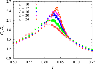
Figure 1: (Color online) Simulation results for the configurational specific heat, obtained with different sample sizes $L$; the statistical errors (not shown) range between 1 and 5%. Meaning of symbols: red crosses: $L=10$; green squares: $L=12$; blue circles: $L=16$; magenta triangles: $L=20$; red diamonds: $L=24$.

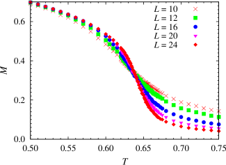
Figure 2: (Color online) Simulation estimates for the mean staggered magnetization $M$, obtained with different sample sizes; here and in the following figures, the errors fall within symbol size; same meaning of symbols as in FIG. 1.

As in our previous paper Chamati and Romano (2014), and as anticipated in Section II, analysis of simulation results showed that, in the ordered region, the staggered magnetization vector $\mathbf{C}$ remains aligned to a lattice main axis: for example, at $T\leq 0.05$, the component of $\mathbf{m}$ largest in magnitude was found to be $\geq 0.95$. As mentioned in the Introduction, a spin wave treatment predicts orientational order at finite temperature, and the prediction was later mathematically justified in Giuliani (2009): the present simulation results are consistent with a spin wave picture of low–temperature excitations.

Results for the mean staggered magnetization $M$, plotted in FIG. 2, were found to decrease with temperature at fixed sample size. For temperatures below 0.5 the data for different sample sizes practically coincide, while for larger temperatures the magnetization decreases significantly as the system size increases. The fluctuations of $M$ versus temperature are investigated trough the susceptibility $\chi$, shown in FIG. 3. We observed a pronounced growth of this quantity with the system size at about $T=0.65$. This is manifested by a significant increase in the maximum height, as well as a shrinking of the “full width at half maximum”, suggesting that the susceptibility will show a singularity as the system size goes to infinity. This behavior is an evidence of the onset of a second order phase transition.

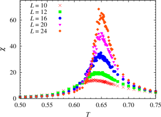
Figure 3: (Color online) Simulation estimates for the susceptibility $\chi$ associated with the staggered magnetization $M$, obtained with different sample sizes; same meaning of symbols as in FIG. 1.

To extract the critical behavior of our model a detailed FSS analysis was applied first to the simulation data obtained for the staggered magnetization $M$ (FIG. 2). This aimed at collapsing all simulation measurements into a single curve describing the behavior of the corresponding scaling function according to the scaling law

$$M=L^{-\beta/\nu}\Theta_{M}\left(tL^{1/\nu}\right);$$ (16)

here $t=1-\tfrac{T}{T_{c}}\ll 1$ denotes the distance from the bulk critical temperature $T_{c}$, $\beta>0$ the critical exponent related to $M$ in the bulk limit i.e. $\lim_{L\to\infty}M\sim t^{\beta}$, and $\nu$ is the critical exponent for the correlation length $\xi$, i.e. $\xi\sim t^{-\nu}$; the function $\Theta_{M}(x)$ is a universal function depending on the gross features of the system, but not on its microscopic details.

To get the best estimates for the critical exponents, several attempts have been made on different sets of sample sizes following closely the procedure explained in Ref. Chamati and Romano (2014), which is based on the minimization approach of Ref. Melchert (2009). The quality of the fit was controlled by a parameter $S$ that was found to range between the values $1$ and $2$ for all quantities considered below. The behavior of the resulting scaling function for the staggered magnetization is reported in FIG. 4 with the critical temperature $T_{c}=0.655\pm 0.001$ and critical exponents $\beta=0.38\pm 0.03$ and $\nu=0.69\pm 0.03$.

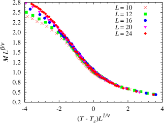
Figure 4: (Color online) Scaling behavior of the staggered magnetization $M$; same meaning of symbols as in FIG. 1.

A similar analysis was performed on the simulation data for the susceptibility $\chi$ leading to $T_{c}=0.655\pm 0.001$ and critical exponents $\gamma=1.31\pm 0.05$ and $\nu=0.74\pm 0.01$. Here we anticipate that, due the large fluctuations of the susceptiblity in the vicinity of the critical temperature (see e.g. FIG. 3), this result may be incorrect. The fitting procedure was attempted on the specific heat as well resulting in $T_{c}=0.652\pm 0.003$, $\alpha=0.13\pm 0.02$ and $\nu=0.69\pm 0.03$. These results indicate that accounting for the dipolar full-range interaction affects both nonuniversal quantities, such as the critical temperature, and universal features, i.e. critical exponents of various thermodynamic quantities. It is worth mentioning that a similar behavior is found in spin systems with algebraically decaying long-range interactions of ferromagnetic type (see e.g. Ref. Chamati and Tonchev (2003) and references therein also covering the bulk case).

Simulation estimates for the fourth-order Binder cumulant $U_{L}$ are shown on FIG. 5. The plots for the different curves are found to decrease against the temperature and to intersect at about $T=0.65$. A FSS of this quantity yields the critical temperature to a very good approximation, since a data collapse leads a scaling function that is independent on the sample size. This is found to be $T_{c}=0.656\pm 0.002$ and the critical exponent $\nu=0.69\pm 0.08$. At the critical temperature we obtain the critical amplitude $U_{L}^{*}\approx 0.54$.

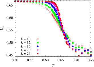
Figure 5: (Color online) Simulation results for the fourth-order Binder cumulant of the staggered magnetization Chamati and Romano (2014) obtained with different sample sizes; same meaning of symbols as in FIG. 1.

At all investigated temperatures, simulation results for the nematic order parameters $\overline{P}_{2}$ and $\overline{P}_{4}$ (FIGs. 6 and 7) exhibited a gradual and monotonic decrease with temperature, vanishing above $T_{c}$, and appeared to be mildly affected by sample sizes; results for $\overline{P}_{4}$ became negligible in the transition region, $T\gtrsim 0.55$ (not shown); in the low–temperature region, simulation results for both observables tended to saturate to 1 as $T\rightarrow 0^{+}$.

According to FSS approach the nematic order parameter is expected to scale like

$$\overline{P}_{2}=L^{-2\beta/\nu}\Xi\left(tL^{1/\nu}\right).$$ (17)

Applying the above mentioned minimization procedure we get $T_{c}=0.655\pm 0.002$, $\beta=0.37\pm 0.02$ and $\nu=0.69\pm 0.03$ in a very good agreement with the above finding for the staggered magnetization.

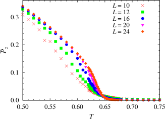
Figure 6: (Color online) Simulation results for the nematic second–rank order parameter $\overline{P}_{2}$, obtained with different sample sizes: same meaning of symbols as in FIG. 1.

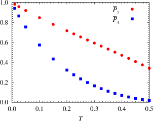
Figure 7: (Color online) Comparison between simulation results for nematic second– and fourth–rank order parameters, in the low–temperature region, and obtained with the largest investigated sample size $L=24$; meaning of symbols: red circles: $\overline{P}_{2}$; blue squares: $\overline{P}_{4}$

Simulation data for $\phi$ [Eq. (15)] are plotted in FIG. 8; for all investigated sample sizes they appear to decrease with increasing temperature; moreover, the results exhibit a recognizable increase of $\phi$ with increasing sample size for $T\lesssim T_{1}=0.64$, and its recognizable decrease with increasing sample size for $T\gtrsim T_{2}=0.68$, so that the seemingly continuous change across the transition region becomes steeper and steeper as sample size increases. In the crossover temperature range between $T_{1}$ and $T_{2}$ the sample–size dependence of results becomes rather weak, and the various curves come close to coincidence at $T\approx 0.66\pm 0.01$, with $~{}\phi\approx 0.54$; notice that this temperature value is in reasonable agreement with $T_{c}$ as independently estimated via the above FSS treatment.

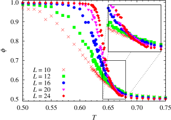
Figure 8: (Color online) Simulation results for the quantity $\phi$, as defined in the text (Eq. 15), obtained with different sample sizes; same meaning of symbols as in FIG. 1.

Let us recall that, by construction, the quantity $\phi$ should be size independent at the critical temperature and thus all curves should coincide there, as it is the case for the Binder cumulant. A FSS analysis was carried out, and found to support this conjecture, giving results consistent with those for $U_{L}$.

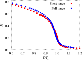
Figure 9: (Color online) Plots of $M$ versus $T/T_{c}$ for the present model and its nearest–neighbor counterpart Chamati and Romano (2014); meaning of symbols: blue circles: present full–range model; red squares: nearest–neighbor counterpart. Both here and in the following FIG. 10, the plotted simulation results had been obtained for $L=24$.

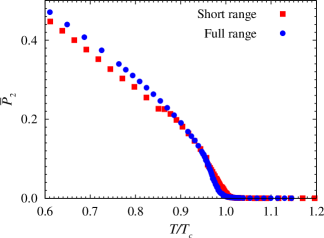
Figure 10: (Color online) Plots of $\overline{P}_{2}$ versus $T/T_{c}$ for the present model and its nearest–neighbor counterpart Chamati and Romano (2014); same meaning of symbols: as in FIG. 9.

To summarize, we propose for the critical temperature the value $T_{c}=655\pm 0.005$, versus the corresponding value $1.877\pm 0.001$ in Ref. Chamati and Romano (2014), thus the ratio $\rho=T_{c}/\left|W_{GS}\right|$ drops to roughly one half of its short–range counterpart ($\approx 0.24$ versus $\approx 0.470$), and this suggests that the long–range tail of the interaction reduces the stability range of the ordered phase in comparison with the nearest–neighbor case. Comparison with the short–range counterpart was also realized in FIGs. 9 and 10, where simulation results for M and $\overline{P}_{2}$, obtained with the largest sample–size used in both studies ($L=24$), are plotted versus $T/T_{c}$; the Figures show a pronounced similarity, as well as a mild but recognizable strengthening of orientational order in the low–temperature region.

On the other hand the critical behavior was found to be governed by the critical exponents $\nu=0.69\pm 0.08$, $\beta=0.38\pm 0.03$ and $\alpha=0.13\pm 0.02$. Except for the above result $\gamma=1.31\pm 0.05$, these values are in agreement with previous Renormalization Group (RG) calculations for isotropic dipolar criticality (Table I in Ref. Bruce and Aharony (1974)), as well as the experimental measurements of Ref. Kumar and Kaul (2015) on Cr₇₀Fe₃₀, obtained on films of appropriate thickness. Since the value of $\gamma$ is highly affected by large fluctuations in the critical region, in order to get a meaningful result we employed the hyperscaling relations to obtain $\gamma\approx 1.37$. Thus the model investigated here is consistent with the isotropic dipolar universality class; comparison between transitional properties for the present model and for its nearest–neighbor counterpart is summarized in the following Table.

Table 1: Comparison between transitional properties for the present model and its nearest–neighbor counterpart Chamati and Romano (2014).

	Present model	Ref. Chamati and Romano (2014)
$W_{GS}$	$-2.676$	$-4$
$T_{c}$	$0.655\pm 0.005$	$1.877\pm 0.001$
$\rho=\tfrac{T_{c}}{\left|W_{GS}\right|}$	$\approx 0.24$	$\approx 0.470$
$\alpha$	$0.13\pm 0.02$	$0.13\pm 0.02$
$\beta$	$0.38\pm 0.03$	$0.358\pm 0.006$
$\gamma$	$\approx 1.37$	$1.4\pm 0.1$
$\nu$	$0.69\pm 0.08$	$0.713\pm 0.001$

As for comparison with other treatments, let us first mention that a Weiss–type Molecular Field approach predicts a transition temperature $T_{c,MF}=\tfrac{2}{3}\left|W_{GS}\right|$, i.e. $\tfrac{8}{3}\approx 2.667$ for the nearest–neighbor counterpart, and $1.784$ in the present case Johnston (2016); Romano (1986a), hence the ratio $T_{c}/T_{c,MF}=\tfrac{3}{2}\rho$ has dropped by the same numerical factor (nearly 2) as above.

Both nearest–neighbor and full–ranged cases of the model investigated here had been studied some sixty years ago by the spherical model (SM) approach Berlin and Kac (1952); Lax (1952); Berlin and Thomsen (1952); Rosenberg and Lax (1953); Toupin and Lax (1957); as for the nearest–neighbor case, the estimated transition temperature can be obtained from Eq. (32) in Berlin and Thomsen (1952) by evaluating a multiple integral numerically, i.e. $T_{c,SM}=1.693$. In the full–ranged case, as far as we could check, Ref. Lax (1952) did not report any explicit numerical estimate of the transition temperature in their Eq. (6.1); on the other hand, some results are available in Ref. Toupin and Lax (1957), via their Eq. (1.3) (with their $\alpha$ set to $0$) and following treatment [see also their FIGs. (1) and (2)]; these results read $F(\lambda_{M})\approx 0.73$, and hence $T_{c,SM}\approx 0.457$.

The critical exponents reported in the above papers were $\beta=\tfrac{1}{2}$ and $\alpha=0$ for both cases: in both cases the configurational specific heat $C_{V}/k_{B}$ was found to remain constant at $\tfrac{3}{2}$ for $T\leq T_{c,SM}$, and to change continuously but with a discontinuous slope at $T=T_{c,SM}$.

An interaction model defined by an extension of (1) had later been studied in Fakioǧlu, S. (1980) by RG; the interaction potential was defined by

$$W_{ij} = \epsilon[-(1+2\sigma)(3+2\sigma)(\mathbf{u}_{i}\cdot\hat{\mathbf{r}}_{ij})(\mathbf{u}_{j}\cdot\hat{\mathbf{r}}_{ij})$$ (18)

$$+(1+2\sigma)(\mathbf{u}_{i}\cdot\mathbf{u}_{j})]/r^{3+\sigma},~{}$$

where $\sigma\geq 0$ is a real parameter: all critical exponents with the exception of $\beta$ were found to depend on $\sigma$, and the limiting case $\sigma=0$ corresponded to the model studied here, for which Eqs. (47) in the named paper Fakioǧlu, S. (1980) yield $\alpha=1$, $\beta=\tfrac{1}{2}$, $\nu=1$, $\eta=2$, $\gamma=0$.

V Conclusions

We have studied here the transitional behavior resulting from the full–ranged counterpart of the lattice–spin model in Refs. Chamati and Romano (2014); Romano (1994a), by means of simulation as well as a detailed analysis of results; FSS basically suggests a universality class with critical exponents $\nu=0.69\pm 0.08$, $\beta=0.38\pm 0.03$ and $\alpha=0.13\pm 0.02$, and a critical temperature $T_{c}=0.655\pm 0.005$, i.e. consistent with an isotropic dipolar critical point Kumar and Kaul (2015); Bruce and Aharony (1974) and different from the nearest–neighbor ferromagnetic Heisenberg one; analysis of second–rank properties has shown the existence of secondary nematic order, destroyed by ground state degeneracy but restored the low–temperature phase, through a mechanism of order by disorder (see Ref. Chamati and Romano (2014) and others quoted therein).

The ratio $\rho=T_{c}/\left|W_{GS}\right|$ drops to roughly one half of its short–range counterpart ($\approx 0.24$ versus $\approx 0.470$) and this suggests that the long–range tail of the interaction reduces the stability range of the ordered phase in comparison with the nearest–neighbor case.

Appendix A Nematic second– and fourth–rank order parameters

Both second– and fourth–rank nematic order parameters Zannoni (1979a, b, 2000) were calculated by analyzing one configuration every cycle; in other words, for a generic examined configuration, the Q tensor is defined by the appropriate generalization of Eq. (11), now involving all the spins in the sample, i.e.

$$Q_{\iota\kappa}=\tfrac{1}{2}(3F_{\iota\kappa}-\delta_{\iota\kappa}),$$ (19)

with

$$F_{\iota\kappa}=\langle u_{\iota}u_{\kappa}\rangle_{loc}=\frac{1}{N}\sum_{j=1}^{N}\left(u_{j,\iota}u_{j,\kappa}\right);$$ (20)

here $\langle\ldots\rangle_{loc}$ denotes average over the current configuration. The fourth-rank order parameter was determined via the analogous quantity Chiccoli et al. (1988)

$$B_{\iota\kappa\lambda\mu} = \frac{1}{8}[35G_{\iota\kappa\lambda\mu}-5(\delta_{\iota\kappa}F_{\lambda\mu}+\delta_{\iota\lambda}F_{\kappa\mu}+\delta_{\iota\mu}F_{\kappa\lambda}$$ (21)

$$+\delta_{\kappa\lambda}F_{\iota\mu}+\delta_{\kappa\lambda}F_{\iota\mu}+\delta_{\lambda\mu}F_{\iota\kappa})$$

$$+(\delta_{\iota\kappa}\delta_{\lambda\mu}+\delta_{\iota\lambda}\delta_{\kappa\mu}+\delta_{\iota\mu}\delta_{\kappa\lambda})],$$

where

$$G_{\iota\kappa\lambda\mu}=\langle u_{\iota}u_{\kappa}u_{\lambda}u_{\mu}\rangle_{loc}=\frac{1}{N}\sum_{j=1}^{N}u_{j,\iota}u_{j,\kappa}u_{j,\lambda}u_{j,\mu}.$$ (22)

The calculated tensor Q was diagonalized; let $\omega_{k}$ denote its three eigenvalues, and let $\mathbf{v}_{k}$ denote the corresponding eigenvectors; the eigenvalue with the largest magnitude (usually a positive number, thus the maximum eigenvalue), can be identified, and its average over the simulation chain defines the nematic second–rank order parameter $\overline{P}_{2}$; the corresponding eigenvector defines the local (fluctuating or “instantaneous”) configuration director $\mathbf{n}$ Zannoni (1979a, b, 2000), evolving along the simulation. Moreover, a suitable reordering of eigenvalues (and hence of the corresponding eigenvectors) is needed for evaluating $\overline{P}_{4}$; let the eigenvalues $\omega_{k}$ be reordered (permuted according to some rule), to yield the values $\omega_{k}^{\prime}$; the procedure used here as well as in other previous papers (e.g. Refs. Hashim et al. (1993); Romano (1994c)) involves a permutation such that

$$|\omega_{3}^{\prime}|\geq|\omega_{1}^{\prime}|,~{}|\omega_{3}^{\prime}|\geq|\omega_{2}^{\prime}|;$$ (23a)

actually there exist two such possible permutations, an odd and an even one; we consistently chose permutations of the same parity (say even ones, see also below) for all examined configurations; recall that eigenvalue reordering also induces the corresponding permutation of the associated eigenvectors. Notice also that, in most cases, $$\omega_{3}^{\prime}>0$$, so that the condition in Eq. (23a) reduces to

$$\omega_{3}^{\prime}\geq\omega_{1}^{\prime},~{}\omega_{3}^{\prime}\geq\omega_{2}^{\prime};$$ (23b)

this latter procedure was considered in earlier treatments of the method. As already mentioned, the second–rank order parameter $\overline{P}_{2}$ is defined by the average of $\omega_{3}^{\prime}$ over the simulation chain; on the other hand, the quantity $(\omega_{2}^{\prime}-\omega_{1}^{\prime})$, and hence its average over the chain, measure possible phase biaxiality, found here to be zero within statistical errors, as it should. The procedure outlined here was previously used elsewhere Hashim et al. (1993); Romano (1994c, 2002a, 2002b, 2003a, 2003b), in cases where some amount of biaxial order might exist; the consistent choice of permutations of the same parity was found to avoid both artificially enforcing a spurious phase biaxiality (as would result by imposing an additional condition such as $|\omega_{1}^{\prime}|\leq|\omega_{2}^{\prime}|$ ), and artificially reducing or even quenching it (as would result by ordering $\omega_{1}^{\prime}$ and $\omega_{2}^{\prime}$ at random).

The fourth-rank order parameter was evaluated from the B tensor in the following way Chiccoli et al. (1988): for each analyzed configuration, the suitably reordered eigenvectors of Q define the director frame, and build the column vectors of an orthogonal matrix R, in turn employed for transforming B to the director frame; the diagonal element $B_{3333}^{\prime}$ of the transformed tensor was averaged over the production run, and identified with $\overline{P}_{4}$.

References

- Note (1) Both electrostatic and magnetostatic dipolar interactions have the same mathematical structure (within numerical factors and usage of different units or symbols), and both interpretations are currently used in the Literature; in the following, we shall be using the magnetic language.
- K. De’Bell and MacIsaac, A. B. and Whitehead, J. P. (2000) K. De’Bell and MacIsaac, A. B. and Whitehead, J. P., “Dipolar effects in magnetic thin films and quasi-two-dimensional systems,” Rev. Mod. Phys. 72, 225 (2000).
- Kaul (2005) S. N. Kaul, “Critical Behaviour of Heisenberg Ferromagnets with Dipolar Interactions and Uniaxial Anisotropy,” in Local-Moment Ferromagnets, Lecture Notes in Physics, Vol. 678, edited by M. Donath and W. Nolting (Springer-Verlag, Berlin, 2005) pp. 9–29.
- Shand et al. (2008) P. M. Shand, J. G. Bohnet, J. Goertzen, J. E. Shield, D. Schmitter, G. Shelburne, and D. L. Leslie-Pelecky, “Magnetic behavior of melt-spun gadolinium,” Phys. Rev. B 77, 184415 (2008).
- Kumar and Kaul (2015) B. R. Kumar and S.N. Kaul, “Magnetic order-disorder phase transition in Cr70Fe30 thin films,” J. Alloys Compd. 652, 479 (2015).
- Bruce and Aharony (1974) A. D. Bruce and A. Aharony, “Critical exponents of ferromagnets with dipolar interactions: Second-order expansion,” Phys. Rev. B 10, 2078 (1974).
- Frey and Schwabl (1991) E. Frey and F. Schwabl, “Renormalized field theory for the static crossover in isotropic dipolar ferromagnets,” Physical Review B 43, 833 (1991).
- Ried et al. (1995) K. Ried, Y. Millev, M. Fähnle, and H. Kronmüller, “Phase transitions in ferromagnets with dipolar interactions and uniaxial anisotropy,” Phys. Rev. B 51, 15229 (1995).
- Meloche et al. (2011) E. Meloche, J. I. Mercer, J. P. Whitehead, T. M. Nguyen, and M. L. Plumer, “Dipole-exchange spin waves in magnetic thin films at zero and finite temperature: Theory and simulations,” Phys. Rev. B 83, 174425 (2011).
- Mól and Costa (2014) L. A. S. Mól and B. V. Costa, “The phase transition in the anisotropic Heisenberg model with long range dipolar interactions,” J. Magn. Magn. Mater. 353, 11 (2014).
- Wysin et al. (2015) G. M. Wysin, A. R. Pereira, W. A. Moura-Melo, and C. I. L. de Araujo, “Order and thermalized dynamics in Heisenberg-like square and Kagomé spin ices,” J. Phys. Condens. Mat. 27, 076004 (2015).
- Belobrov et al. (1983) P. I. Belobrov, R. S. Gekht, and V. A. Igantchenko, “Ground state in systems with dipole interaction,” Sov. Phys. JETP 57, 636–642 (1983).
- Cohen and Keffer (1955) M. H. Cohen and F. Keffer, “Dipolar Ferromagnetism at 0 K,” Phys. Rev. 99, 1135 (1955).
- Sullivan et al. (1974) D. E. Sullivan, J. M. Deutch, and G. Stell, “Thermodynamics of polar lattices,” Mol. Phys 28, 1359 (1974).
- Adams and McDonald (1976) D. J. Adams and I. R. McDonald, “Thermodynamic and dielectric properties of polar lattices,” Mol. Phys 32, 931 (1976).
- Chamati and Romano (2014) H. Chamati and S. Romano, “Nematic order by thermal disorder in a three–dimensional lattice–spin model with dipolar–like interactions,” Phys. Rev. E 90, 022506 (2014).
- Schönke et al. (2015) J. Schönke, T. M. Schneider, and I. Rehberg, “Infinite geometric frustration in a cubic dipole cluster,” Phys. Rev. B 91, 020410 (2015).
- Holden et al. (2015) M. S. Holden, M. L. Plumer, I. Saika-Voivod, and B. W. Southern, “Monte Carlo simulations of a kagome lattice with magnetic dipolar interactions,” Phys. Rev. B 91, 224425 (2015).
- Johnston (2016) D. C. Johnston, “Magnetic dipole interactions in crystals,” Phys. Rev. B 93, 014421 (2016).
- Giuliani (2009) A. Giuliani, “Long range order for lattice dipoles,” J. Stat. Phys. 134, 1059 (2009).
- Fröhlich and Spencer (1981) J. Fröhlich and T. Spencer, “On the statistical mechanics of classical coulomb and dipole gases,” J. Stat. Phys. 24, 617 (1981).
- Fröhlich et al. (1978) J. Fröhlich, R. Israel, E. H. Lieb, and B. Simon, “Phase transitions and reflection positivity. I. General theory and long range lattice models,” Commun. Math. Phys. 62, 1 (1978).
- Romano (1986a) S. Romano, “Computer simulation study of a simple-cubic dipolar lattice,” Nuov. Cim. D 7, 717 (1986a).
- Romano (1986b) S. Romano, “Computer simulation study of the singlet orientational distribution function for a model antiferroelectric nematic,” Europhys. Lett. 2, 431 (1986b).
- Romano (1994a) S. Romano, “Computer-simulation study of a three-dimensional lattice-spin model with dipolar-type interactions,” Phys. Rev. B 49, 12287 (1994a).
- Zannoni (1979a) C. Zannoni, “Distribution function and order parameters,” in The molecular physics of liquid crystals, edited by G. R Luckhurst and G. W Gray (Academic Press, London, 1979) Chap. 3, p. 51.
- Zannoni (1979b) C. Zannoni, “Computer simulations,” in The molecular physics of liquid crystals, edited by G. R Luckhurst and G. W Gray (Academic Press, London, 1979) Chap. 9, p. 191.
- Zannoni (2000) C. Zannoni, “Liquid Crystal Observables: Static and Dynamic Properties,” in Advances in the Computer Simulatons of Liquid Crystals, NATO Science Series No. 545, edited by P. Pasini and C. Zannoni (Springer, Dordrecht, 2000) p. 17.
- Villain et al. (1980) J. Villain, R. Bidaux, J.-P. Carton, and R. Conte, “Order as an effect of disorder,” J. Physique 41, 1263 (1980).
- Henley (1989) C. L. Henley, “Ordering due to disorder in a frustrated vector antiferromagnet,” Phys. Rev. Lett. 62, 2056–2059 (1989).
- Prakash and Henley (1990) S. Prakash and C. L. Henley, “Ordering due to disorder in dipolar magnets on two-dimensional lattices,” Phys. Rev. B 42, 6574 (1990).
- Romano (1994b) S. Romano, “Computer simulation study of a two-dimensional lattice spin model with interactions of dipolar type,” Phys. Scr. 50, 326 (1994b).
- Yamaguchi and Okabe (2001) C. Yamaguchi and Y. Okabe, “Three-dimensional antiferromagnetic q-state Potts models: application of the Wang-Landau algorithm,” J. Phys. A: Math. Gen. 34, 8781 (2001).
- Romano and De Matteis (2011) S. Romano and G. De Matteis, “Orientationally ordered phase produced by fully antinematic interactions: A simulation study,” Phys. Rev. E 84, 011703 (2011).
- Biskup et al. (2004) M. Biskup, L. Chayes, and S. A. Kivelson, “Order by Disorder, without Order, in a Two-Dimensional Spin System with O(2) Symmetry,” Ann. Henri Poincaré 5, 1181 (2004).
- Allen and Tildesley (1989) M. P. Allen and D. J. Tildesley, Computer Simulation of Liquids (Oxford University Press, 1989).
- Frenkel and Smit (1996) D. Frenkel and B. Smit, Understanding Molecular Simulation From Algorithms to Applications (Academic Press, San Diego, CA, 1996).
- Barker and Watts (1969) J. A. Barker and R. O. Watts, “Structure of water: a monte carlo calculation,” Chem. Phys. Lett. 3, 144–145 (1969).
- Paauw et al. (1975) Th. T. A. Paauw, A. Compagner, and D. Bedeaux, “Monte-Carlo calculation for the classical F.C.C. Heisenberg ferromagnet,” Physica A 79, 1 (1975).
- Peczak et al. (1991) P. Peczak, A. M. Ferrenberg, and D. P. Landau, “High accuracy monte carlo study of the three-dimensional classical heisenberg ferromagnet,” Phys. Rev. B 43, 6087 (1991).
- Binder (1981) K. Binder, “Finite size scaling analysis of ising model block distribution functions,” Z. Phys. B 43, 119 (1981).
- Melchert (2009) O. Melchert, “autoScale.py - a program for automatic finite-size scaling analyses: A user’s guide,” (2009), arXiv:0910.5403 [physics.comp-ph] .
- Chamati and Tonchev (2003) H. Chamati and N. S. Tonchev, “Critical behavior of systems with long-range interaction in restricted geometry,” Mod. Phys. Lett. B 17, 1187 (2003).
- Berlin and Kac (1952) T. H. Berlin and M Kac, “The spherical model of a ferromagnet,” Phys. Rev. 86, 821 (1952).
- Lax (1952) M. Lax, “Dipoles on a lattice: the spherical model,” J. Chem. Phys. 20, 1351 (1952).
- Berlin and Thomsen (1952) T. H. Berlin and J. S. Thomsen, “Dipole-dipole interaction in simple lattices,” J. Chem. Phys. 20, 1368 (1952).
- Rosenberg and Lax (1953) R. Rosenberg and M. Lax, “High temperature susceptibility of permanent dipole lattices,” J. Chem. Phys. 21, 424 (1953).
- Toupin and Lax (1957) R. A. Toupin and M. Lax, “Lattice of partly permanent dipoles,” J. Chem. Phys. 27, 458 (1957).
- Fakioǧlu, S. (1980) Fakioǧlu, S., “Renormalization group and critical exponents for classical heisenberg ferromagnet with dipole-dipole interactions,” Phys. Stat. Sol. B 98, 307 (1980).
- Chiccoli et al. (1988) C. Chiccoli, P. Pasini, F. Biscarini, and C. Zannoni, “The model and its orientational phase transition,” Mol. Phys. 65, 1505–1524 (1988).
- Hashim et al. (1993) R. Hashim, G. R. Luckhurst, F. Prata, and S. Romano, “Computer simulation studies of anisotropic systems. XXII. An equimolar mixture of rods and discs: A biaxial nematic?” Liq. Cryst. 15, 283 (1993).
- Romano (1994c) S. Romano, “Computer simulation study of a three-dimensional lattice spin model with anti-nematic interactions,” Int. J. Mod. Phys. B 8, 3389 (1994c).
- Romano (2002a) S. Romano, “Computer simulation study of a two-dimensional nematogenic lattice model based on the Gruhn-Hess interaction potential,” Phys. Lett. A 302, 203 (2002a).
- Romano (2002b) S. Romano, “Computer simulation study of a two-dimensional nematogenic lattice model based on the Nehring-Saupe interaction potential,” Phys. Lett. A 305, 196 (2002b).
- Romano (2003a) S. Romano, “Computer simulation study of two-dimensional nematogenic lattice models based on dispersion interactions,” Physica A 322, 432 (2003a).
- Romano (2003b) S Romano, “Computer simulation study of a two-dimensional nematogenic lattice model based on a mapping from elastic free-energy density,” Phys. Lett. A 310, 465 (2003b).