Effective numerical treatment of sub-diffusion equation with non-smooth solution

Abstract

In this paper we investigate a sub-diffusion equation for simulating the anomalous diffusion phenomenon in real physical environment. Based on an equivalent transformation of the original sub-diffusion equation followed by the use of a smooth operator, we devise a high-order numerical scheme by combining the Nyström method in temporal direction with the compact finite difference method and the spectral method in spatial direction. The distinct advantage of this approach in comparison with most current methods is its high convergence rate even though the solution of the anomalous sub-diffusion equation usually has lower regularity on the starting point. The effectiveness and efficiency of our proposed method are verified by several numerical experiments. Keywords: fractional derivative; anomalous sub-diffusion; weakly singular; Volterra integral equation; spectral method

1 Introduction

Fractional calculus is an area having a long history, which is believed to have stemmed from a question about the meaning of notation $d^{\frac{1}{2}}y/dx^{\frac{1}{2}}$ raised in the year 1695 by Marquis de L’Hôpital to Gottfried Wihelm Leibniz. During the past three decades, this subject has gained considerable popularity due mainly to its powerful applications in numerous seemingly diverse and widespread fields of science and engineering, such as materials and mechanics, signal processing, anomalous diffusion, biological systems, finance, and etc.(see [19, 18, 12, 2, 11, 10]). At present there have been many papers presenting fractional calculus models for kinetics of natural anomalous processes in complex systems. These models always maintain the long-memory and non-local properties of the corresponding dynamics. Because of these properties, it is still not easy to find the exact or numerical solutions of these equations, though researchers have developed many methods to approach this goal. Special interest has been paid to the anomalous diffusion processes, which include super-slow diffusion (or sub-diffusion) and super-fast diffusion (or super-diffusion). Among those models, anomalous sub-diffusion equations are important due to its application in simulating real physical sub-diffusion phenomena. The model is always written as

$$\left\{\begin{aligned} &u_{t}(x,t)=\prescript{RL}{0}{\mathcal{D}}^{1-\gamma}_{t}Lu(x,t)+\bar{f}(x,t),&0<x\leq X,\,0<t\leq T,\\ &u(x,0)=\varphi(x),&0\leq x\leq X,\\ &u(0,t)=\psi_{1}(t),\quad u(X,t)=\psi_{2}(t),&0\leq t\leq T,\\ \end{aligned}\right.$$

where $0<\gamma<1$, $Lu(x,t)=K_{\gamma}u_{xx}(x,t)$ and $\prescript{RL}{0}{\mathcal{D}}^{1-\gamma}_{t}$ denotes the Riemann-Liouville fractional derivative of order $1-\gamma$,

$$\prescript{RL}{0}{\mathcal{D}}^{1-\gamma}_{t}u(x,t)=\frac{1}{\Gamma(\gamma)}\frac{\partial}{\partial t}\int_{0}^{t}(t-\eta)^{\gamma-1}u(x,\eta)\,d\eta.$$ (1.1)

Assume $\bar{f}=\prescript{RL}{0}{\mathcal{D}}^{1-\gamma}_{t}f$, then we can rewrite the original equation as below[12]:

$$\left\{\begin{aligned} &u_{t}(x,t)=\prescript{RL}{0}{\mathcal{D}}^{1-\gamma}_{t}\big{(}Lu(x,t)+f(x,t)\big{)},&0<x\leq X,\,0<t\leq T,\\ &u(x,0)=\varphi(x),&0\leq x\leq X,\\ &u(0,t)=\psi_{1}(t),\quad u(X,t)=\psi_{2}(t),&0\leq t\leq T.\end{aligned}\right.$$ (1.2)

In this paper we only consider anomalous sub-diffusion problem in form (1.2). In some references, equation (1.2) is called the time Riemann-Liouville type sub-diffusion equation. Some researchers use the following models instead of equation (1.2) :

$$\prescript{RL}{0}{\mathcal{D}}^{\gamma}_{t}(u(x,t)-u(x,0))=Lu(x,t)+f(x,t),$$ (1.3)

or

$$\prescript{C}{0}{\mathcal{D}}^{\gamma}_{t}u(x,t)=Lu(x,t)+f(x,t),$$ (1.4)

where $\prescript{C}{0}{\mathcal{D}}^{\gamma}_{t}$ denotes the Caputo fractional derivative of order $\gamma$,

$$\prescript{C}{0}{\mathcal{D}}^{\gamma}_{t}u(x,t)=\frac{1}{\Gamma(1-\gamma)}\int_{0}^{t}(t-\eta)^{-\gamma}\frac{\partial}{\partial\eta}u(x,\eta)\,d\eta.$$ (1.5)

In fact, these models are equivalent. Many numerical methods have been developed to solve anomalous sub-diffusion equations. In 2005, Yuste and Scedo[17] proposed an explicit FTCS scheme, which combined the forward time centered space (FTCS) method with the Grünwald-Letnikov discretization of the Riemann-Liouville derivative. And a new von Neumann-type method is applied to analysis the stability in the paper. Zhuang et al.[22] presented an implicit numerical method as well as two techniques which are used to improve the order of convergence. The stability and convergence analysis for the implicit numerical method are given by using an energy method. Combining the L1 discretization for time-fractional part and fourth-order accuracy compact approximation for space derivative, a compact finite difference scheme is established by Gao and Sun[9]. Furthermore, Gao et al.[8] offered a scheme with global second-order numerical accuracy in time independent of the fractional derivative exponent. Apart from finite difference methods, part of researchers have investigated Galerkin methods, including finite element methods and spectral methods. Zeng et al.[20] adopted linear multistep method and finite element method to approach the time-fractional sub-diffusion equation and got two unconditionally stable schemes. Mustapha developed a discontinuous Petrov-Galerkin method[14] and a time-stepping $hp$-versions discontinuous Galerkin method[15] for time fractional partial differential equations. In [7, 6], Dehghan et al. developed spectral element method in spatial and finite difference method in temporal for nonlinear fractional partial differential equations and sub-diffusion equations, and gave the corresponding theoretical analysis. They also studied the homotopy analysis method and the dual reciprocity boundary integral method for fractional partial differential equations[4, 3]. In addition, the authors presented two high-order methods for multi-term time-fractional diffusion equation[5]. For multi-term time-fractional diffusion equation, with the benefit of spectral method, Zheng et al.[21] gained a valuable high-order scheme, which possessing high efficiency and exponential decay in both time and space directions. There have been a great deal of researches on anomalous sub-diffusion equations, however, as noticed in [8], when the solution is not smooth enough at $t=0$, the convergence rate will be lower than expectation. To overcome this shortcoming, we adopt some techniques similar to those used to deal with weakly singularity Volterra integral equation[1, 13]. By these techniques, we can obtain better numerical results even though the solution has weak regularity. The effectiveness of our algorithm can be seen in the numerical examples. The outline of this paper is arranged as follows. In Section 2, we give an equivalent form of equation (1.2) by equivalent transformation and smoothing operator, which can improve the regularity of the solution. Section 3 contains a semi-discrete scheme given by discretizing the equivalent equation with Nyström method. With different method discretizing spatial variables, two fully-discrete schemes are presented in Section 4. To demonstrate the efficiency and effectiveness of the proposed scheme, we perform some numerical examples in Section 5. And in the last section conclusions as well as some remarks are given.

2 Equivalent transformation and smoothing method

In paper [1], the authors proposed a simple smooth transformation for Volterra integral equations, which can improve the regularity of the solution and can be used to construct high-order convergence methods. In this section, we further introduce a smoothing method to transform the original fractional differential equation (1.2) into an equivalent form. In order to use the smoothing method, the equation (1.2) is transformed into an integral equation by integrating both sides:

$$\int_{0}^{s}u_{t}(x,t)\,dt=\int_{0}^{s}\frac{1}{\Gamma(\gamma)}\frac{\partial}{\partial t}\int_{0}^{t}(t-\eta)^{\gamma-1}\big{(}Lu(x,\eta)+f(x,\eta)\big{)}\,d\eta\,dt.$$

Then we have

$$u(x,s)=u(x,0)+\frac{1}{\Gamma(\gamma)}\int_{0}^{s}(s-\eta)^{\gamma-1}\big{(}Lu(x,\eta)+f(x,\eta)\big{)}\,d\eta,$$

i.e.

$$u(x,t)=u(x,0)+\frac{1}{\Gamma(\gamma)}\int_{0}^{t}(t-\eta)^{\gamma-1}\big{(}Lu(x,\eta)+f(x,\eta)\big{)}\,d\eta.$$ (2.1)

The last term in the right hand of (2.1) has a similar form with an integral term in the Volterra integral equation. Following [1], we introduce the smooth operator

$$\lambda(t)=(b-a)^{1-q}(t-a)^{q}+a,\quad q\in\{1,2,\dots,n,\dots\},$$ (2.2)

which maps $[a,b]$ into $[a,b]$ where $a$ is $0$ and $b$ is $T$. Here, we use $a$, $b$ as end points to state the generality of the transformation. Let $\alpha=1-\gamma$ and change the variables in (2.1) by setting $\eta=\lambda(s)$, $t=\lambda(t^{\prime})$. Replacing $t^{\prime}$ by $t$, we then get

$$u(x,\lambda(t))=u(x,\lambda(a))+\frac{1}{\Gamma(\gamma)}\int_{a}^{t}\big{(}\lambda(t)-\lambda(s)\big{)}^{-\alpha}G(x,s)\lambda^{\prime}(s)\,ds,$$ (2.3)

where $G(x,s)=Lu\big{(}x,\lambda(s)\big{)}+f\big{(}x,\lambda(s)\big{)}$. To transform the kernel of (2.3) with form $(t-s)^{-\alpha}$, we denote[1]

$$\delta_{\alpha}(t,s)=\left\{\begin{aligned} &\left(\frac{(t-a)^{q}-(s-a)^{q}}{t-s}\right)^{-\alpha},&t&\neq s,\\ &\big{(}q(s-a)^{q-1}\big{)}^{-\alpha},&t&=s.\end{aligned}\right.$$ (2.4)

The equation (2.4) implies

$$\big{(}\lambda(t)-\lambda(s)\big{)}^{-\alpha} =\big{(}(b-a)^{1-q}\big{)}^{-\alpha}\delta_{\alpha}(t,s)(t-s)^{-\alpha}.$$ (2.5)

Multiplying both sides of (2.3) by $\lambda^{\prime}(t)$, we can now rewrite (2.3) as

$$\lambda^{\prime}(t)u(x,\lambda(t))=\lambda^{\prime}(t)u(x,\lambda(a))+\frac{1}{\Gamma(\gamma)}\int_{a}^{t}(t-s)^{-\alpha}K_{\alpha}(t,s)G(x,s)\lambda^{\prime}(s)\,ds,$$ (2.6)

where

$$K_{\alpha}(t,s)=\big{(}(b-a)^{1-q}\big{)}^{-\alpha}\lambda^{\prime}(t)\delta_{\alpha}(t,s).$$ (2.7)

In order to use the Nyström method in spatial direction, we introduce another transformation $\mu(t)=\frac{b-a}{2}t+\frac{b+a}{2}$ and denote

$$\left\{\begin{aligned} v(x,t)&=\lambda^{\prime}\big{(}\mu(t)\big{)}u\big{(}x,\lambda\big{(}\mu(t)\big{)}\big{)},\\ g(x,t)&=\lambda^{\prime}\big{(}\mu(t)\big{)}f\big{(}x,\lambda\big{(}\mu(t)\big{)}\big{)},\\ h(x,t)&=\lambda^{\prime}\big{(}\mu(t)\big{)}u\big{(}x,\lambda\big{(}a\big{)}\big{)}.\end{aligned}\right.$$ (2.8)

By setting $t=\mu(t^{\prime})$, $s=\mu(s^{\prime})$ in (2.6) and replacing $t^{\prime}$ by $t$, $s^{\prime}$ by $s$, we get

$$v(x,t)=h(x,t)+\frac{1}{\Gamma(\gamma)}\int_{-1}^{t}(t-s)^{-\alpha}H(t,s)\big{(}Lv(x,s)+g(x,s)\big{)}\,ds,$$ (2.9)

where

$$H(t,s)=\left(\frac{b-a}{2}\right)^{1-\alpha}K_{\alpha}\big{(}\mu(t),\mu(s)\big{)}.$$ (2.10)

After two times of transformations, a new equation (2.9) for the problem (1.2) is derived. For equation (2.9), the kernel is $\hat{H}(t,s)=(t-s)^{-\alpha}H(t,s)$. According to the expression, we know $H(t,s)$ is continuous and $\hat{H}(t,s)\in L^{1}([-1,1]\times[-1,1])$ is a weakly singular kernel. Now we consider the smoothness of the solution of the new equation (2.9). Suppose that $u(x,t)\to O(t^{\beta})$ ($\beta>0$) as $t\to 0$. Then $\lambda^{\prime}(s)u(x,\lambda(s))\to O(s^{q\beta+q-1})$ as $s\to 0$. As we set $v(x,t)=\lambda^{\prime}\big{(}\mu(t)\big{)}u\big{(}x,\lambda(\mu(t))\big{)}$ and $\mu(t)$ is the first order polynomial which do not change the smoothness. Then $v(x,t)\to O(t^{q\beta+q-1})$ as $t\to 0$. Obviously, $q\beta+q-1\geq\beta$, i.e. $v(x,t)$ is smoother than $u(x,t)$ when $q>1$. Because the new solution has higher regularity, traditional methods can be applied to solve this equation without loss much accuracy. As a conclusion, we illustrate the smoothing process as below

In the next section, we will describe more details of how to discretize the above equation.

3 The semi-discrete approximation

In the previous section we have obtained an equivalent equation (2.9). Here, we present a semi-discrete scheme by using the Nyström method. Choose $N+1$ distinct points $\tau_{n},n=0,\cdots,N$ in the interval $[-1,1]$ corresponding to $t_{n},n=0,\cdots,N$ in $[a,b]$ with $t_{n}=\lambda\big{(}\mu(\tau_{n})\big{)}$. And collocate the equation at the nodes $\{\tau_{n}\}^{N}_{n=0}$

$$v(x,\tau_{n})=h(x,\tau_{n})+\frac{1}{\Gamma(\gamma)}\int_{-1}^{\tau_{n}}(\tau_{n}-s)^{-\alpha}H(\tau_{n},s)\big{(}Lv(x,s)+g(x,s)\big{)}ds.$$ (3.1)

Then replace $H(\tau_{n},s)\big{(}Lv(x,s)+g(x,s)\big{)}$ by the corresponding Lagrange interpolation polynomials associated with $\{\tau_{n}\}^{N}_{n=0}$

$$v(x,\tau_{n})=h(x,\tau_{n})+\frac{1}{\Gamma(\gamma)}\sum_{j=0}^{N}w_{n,j}H(\tau_{n},\tau_{j})(Lv(x,\tau_{j})+g(x,\tau_{j}))$$ (3.2)

where

$$w_{n,j}=\int_{-1}^{\tau_{n}}(\tau_{n}-s)^{-\alpha}I_{N,j}(s)\,ds,$$

and $I_{N,j}(s)$ are the Lagrange interpolation polynomials on points $\{\tau_{n}\}^{N}_{n=0}$. For the computation of the coefficients of $w_{n,j}$, we use the Jacobi-Gauss quadrature as described in [16].

Remark 3.1.

Because of the singularity of the solution, the point $\tau=-1$ should not be chosen as an element of $\{\tau_{n}\}$.

Remark 3.2.

By choosing different $\{\tau_{n}\}_{n=0}^{n=N}$, we get different approximation polynomials with different accuracies. This will have effect on the accuracy of the solution.

Now, we obtain a semi-discrete scheme for equation (1.2)

$$v(x,\tau_{n})=h(x,\tau_{n})+\sum_{j=0}^{N}r_{nj}(Lv(x,\tau_{j})+g(x,\tau_{j})),\quad n=0,1,\cdots,N,$$ (3.3)

where $r_{nj}=w_{n,j}H(\tau_{n},\tau_{j})/\Gamma(\gamma)$. Once $v(x,\tau)$ is obtained, the solution of the original equation is given by

$$u(x,t)=\frac{v(x,\tau)}{\lambda^{\prime}\big{(}\mu(\tau)\big{)}},\quad t=\lambda\big{(}\mu(\tau)\big{)}.$$ (3.4)

4 The fully-discrete approximation

Because of the high convergence rate in temporal direction of the scheme, we need a high-order method in spatial direction for competence. In this section, we perform two different discrete methods on the spatial variable.

4.1 Discrete spatial variable by compact difference operator

In this subsection, we use spatial compact approximation in spatial direction. Let $x_{k}=k\Delta x,(k=0,1,\cdots,M)$ with step $\Delta x=X/M$. Like [8], denote a average operator

$$\mathcal{A}u_{i}=\left\{\begin{aligned} &(I+\frac{\Delta x^{2}}{12}\delta^{2}_{x})u_{i},&1\leq i\leq M-1,\\ &u_{i},&i=0\ \text{or}\ i=M.\end{aligned}\right.$$ (4.1)

where $\delta_{x}^{2}$ is the centered difference operator. Perform $\mathcal{A}$ on both sides of (3.3) at $\{x_{k}\}_{k=1}^{M-1}$

$$\mathcal{A}v(x_{k},\tau_{n})=\mathcal{A}h(x_{k},\tau_{n})+\sum^{N}_{j=0}r_{nj}\big{(}K_{\gamma}\mathcal{A}v_{xx}(x_{k},\tau_{j})+\mathcal{A}g(x_{k},\tau_{j})\big{)}.$$ (4.2)

The next thing is to approximation $\mathcal{A}v_{xx}(x_{k},s)$. In order to obtain the spatial compact scheme, we need the following lemma, which suggests that $\delta_{x}^{2}v(x_{k},s)$ is a good approximation to $\mathcal{A}v_{xx}(x_{k},s)$.

Lemma 4.1 ([8]).

Let function $g(x)\in C^{6}[0,X]$ and $\xi(\eta)=(1-\eta)^{3}\big{(}5-3(1-\eta)^{2}\big{)}$. Then

$$\mathcal{A}g^{\prime\prime}(x_{i})=\delta^{2}_{x}g(x_{i})+\frac{\Delta x^{4}}{360}\int_{0}^{1}\big{(}g^{(6)}(x_{i}-\eta\Delta x)+g^{(6)}(x_{i}+\eta\Delta x)\big{)}\xi(\eta)\,d\eta.$$ (4.3)

By Lemma 4.1, we have

$$\mathcal{A}v(x_{k},\tau_{n})=\mathcal{A}h(x_{k},\tau_{n})+r_{nj}(K_{\gamma}\delta^{2}_{x}v(x_{k},\tau_{j})+\mathcal{A}g(x_{k},\tau_{j}))+O(\Delta x^{4}).$$ (4.4)

Drop down the high-order term, hence

$$\mathcal{A}v(x_{k},\tau_{n})=\mathcal{A}h(x_{k},\tau_{n})+r_{nj}(K_{\gamma}\delta^{2}_{x}v(x_{k},\tau_{j})+\mathcal{A}g(x_{k},\tau_{j})).$$ (4.5)

Now, we have established the fully-discrete scheme by discrete spatial variables with compact difference operator. To introduce the matrix form of the last scheme, we denote $v_{k}^{n}=v(x_{k},\tau_{n})$, $h_{k}^{n}=h(x_{k},\tau_{n})$, and $g_{k}^{j}=g(x_{k},\tau_{j})$. In addition, let $\bm{V}$, $\bm{V}_{0}$, $\bm{W}$ and $\bm{G}$ be matrix with $(\bm{V})_{k,n+1}=v_{k}^{n}$, $(\bm{V}_{0})_{k,n+1}=h_{k}^{n}$, $(\bm{W})_{n+1,j+1}=r_{nj}$ and $(\bm{G})_{k,n+1}=g_{k}^{n}$  ($k=1,\cdots,M-1$,  $j=0,\cdots,N$,  $n=0,\cdots,N$). Then the matrix form of scheme (4.5) can be written as below:

$$\bm{V}+\frac{1}{12}(\bm{DV}+\bm{B}_{v})= \bm{V}_{0}+\frac{1}{12}(\bm{D}\bm{V}_{0}+\bm{B}_{h})+\frac{K_{\gamma}}{\Delta x^{2}}(\bm{D}\bm{V}+\bm{B}_{v})\bm{W}^{T}$$ (4.6)

$$+\big{(}\bm{G}+\frac{1}{12}(\bm{D}\bm{G}+\bm{B}_{g})\big{)}\bm{W}^{T},$$

where the matrix $\bm{D}$ equals to $\text{tridiag}(1,-2,1)$, and $\bm{B}_{h}$, $\bm{B}_{g}$ are similar to $\bm{B}_{v}$ which is defined as follows:

$$\bm{B}_{v,(M-1)\times(N+1)}=\left(\begin{array}[]{ccccc}v_{0}^{0}&v_{0}^{1}&\cdots&v_{0}^{N-1}&v_{0}^{N}\\ 0&0&\cdots&0&0\\ \vdots&\vdots&\ddots&\vdots&\vdots\\ 0&0&\cdots&0&0\\ v_{M}^{0}&v_{M}^{1}&\cdots&v_{M}^{N-1}&v_{M}^{N}\end{array}\right).$$

. For simplification, we recombine the terms in equation (4.6) as

$$\bm{T}\bm{V}-\bm{A}\bm{V}\bm{W}^{T}=\bm{S},$$ (4.7)

where $\bm{T}=\bm{I}+\frac{1}{12}\bm{D}$, $\bm{A}=\frac{K_{\gamma}}{\Delta x^{2}}\bm{D}$ and

$$\bm{S}=-\frac{1}{12}\bm{B}_{v}+\bm{V}_{0}+\frac{1}{12}(\bm{D}\bm{V}_{0}+\bm{B}_{h})+\big{(}\bm{G}+\frac{1}{12}(\bm{D}\bm{G}+\bm{B}_{g})\big{)}\bm{W}^{T}.$$ (4.8)

Combining (3.4) and (4.7), we can obtain the solution of the original equation.

4.2 Spatial discretization with spectral method

In order to compare the result with some existing algorithms, we use the space basis function, presented by Zheng et al. in [21], to solve equation (3.3). Here, we only consider zero boundary condition, i.e., $u(0,t)=0$, $u(X,t)=0.$ Firstly, let us state the variational problem of equations (3.3). We recall the semi-discrete scheme (3.3)

$$v(x,\tau_{n})=h(x,\tau_{n})+\sum_{j=0}^{N}r_{nj}(Lv(x,\tau_{j})+g(x,\tau_{j}))\quad n=0,1,\cdots,N.$$ (4.9)

Set $v^{n}(x)=v(x,\tau_{n})$, $h^{n}(x)=h(x,\tau_{n})$, $g^{n}(x)=g(x,\tau_{n})$, $\Lambda=[0,X]$. Then the variational problem of (3.3) is : Find $v^{n}(x)\in H_{0}^{1}(\Lambda)$, $(n=0,1,\cdots,N)$ for $\forall\phi(x)\in H_{0}^{1}(\Lambda)$, such that

$$\big{(}v^{n}(x),\phi(x)\big{)}+ \ K_{\gamma}\sum_{j=0}^{N}r_{nj}\big{(}v^{j}_{x}(x),\phi_{x}(x)\big{)}$$ (4.10)

$$=\big{(}h^{n}(x),\phi(x)\big{)}+\sum_{j=0}^{N}r_{nj}\big{(}g^{j}(x),\phi(x)\big{)}.$$

Next, we construct a spectral scheme for the above variational problem. Let $\mathbb{P}_{M^{\prime}}(\Lambda)$ denote the spaces of polynomials of degree up to $M^{\prime}$ and set

$$P_{M^{\prime}}(\Lambda)=\{p(x)\in\mathbb{P}_{M^{\prime}}(\Lambda)|p(0)=p(X)=0\}.$$

Adopt the Fourier-like functions proposed by Zheng et al. [21, see Section 4.2 for more details]. Let

$$\hat{x}=\frac{2}{X}(x-\frac{X}{2}),$$

and define

$$z_{k}(x)=\lambda_{k}(L_{k}(\hat{x})-L_{k+2}(\hat{x})),$$

where $L_{k}(\hat{x})$ is Legendre polynomials and $\lambda_{k}=\sqrt{\frac{X}{4(2k+3)}}$. Then $(z^{\prime}_{i}(x),z^{\prime}_{j}(x))_{\Lambda}=\delta_{ij}$ where $\delta_{ij}$ is the Kronecker delta. Set $Z=\left((z_{i},z_{j})_{\Lambda}\right)_{(M^{\prime}-1)\times(M^{\prime}-1)}$, and let

$$\zeta_{i}(x)=\sum_{i=0}^{N-2}q_{ik}z_{i}(x),\quad k=0,1,\cdots,M^{\prime}-2.$$

where $\{q_{ik}\}_{i=0}^{M^{\prime}-2}$ is the eigenvector corresponding to the eigenvalue $\pi_{k}$ of the matrix $Z$. And the basis functions $\zeta_{i}(x)$ have the following property.

Lemma 4.2 ([21]).

For the basis functions $\zeta_{i}(x)(i=0,1,\cdots,M-2),x\in(a,b)$,

$$(\zeta_{i}(x),\zeta_{j}(x))=\pi_{i}\delta_{ij},\quad(\zeta_{i}^{\prime}(x),\zeta_{j}^{\prime}(x))=\delta_{ij}.$$ (4.11)

Let $v_{L}^{n}=\sum_{i=0}^{M^{\prime}-2}\hat{v}_{i}^{n}\zeta_{i}$, then we obtain the spectral scheme for problem (4.10):

$$\big{(}v^{n}_{L}(x),\zeta_{i}(x)\big{)}+ \ K_{\gamma}\sum_{j=0}^{N}r_{nj}\big{(}v^{j}_{L,x}(x),\zeta_{i}^{\prime}(x)\big{)}$$ (4.12)

$$=\big{(}h^{n}(x),\zeta_{i}(x)\big{)}+\sum_{j=0}^{N}r_{nj}\big{(}g^{j}(x),\zeta_{i}(x)\big{)},$$

$$\qquad\qquad\qquad\qquad\forall i=0,1,\cdots,M^{\prime}-2.$$

Now, we introduce the matrix form of this scheme. Adopt the following notations

$$V^{j}=(\hat{v}_{0}^{j},\hat{v}_{1}^{j},\cdots,\hat{v}_{M^{\prime}-2}^{j})^{T},$$ (4.13)

$$H^{j}=\big{(}(h^{j},\zeta_{0}),(h^{j},\zeta_{1}),\cdots,(h^{j},\zeta_{M^{\prime}-2})\big{)}^{T},$$

$$G^{j}=\big{(}(g^{j},\zeta_{0}),(g^{j},\zeta_{1}),\cdots,(g^{j},\zeta_{M^{\prime}-2})\big{)}^{T}.$$

Then we have

$$\bm{\Pi}V^{n}+K_{\gamma}\sum_{j=0}^{N}r_{nj}V^{j}=H^{n}+\sum_{j=0}^{N}r_{nj}G^{j},\quad n=0,1,\cdots,N,$$ (4.14)

where $\bm{\Pi}=\text{diag}(\pi_{0},\pi_{1},\cdots,\pi_{M^{\prime}-2})$. Also define

$$V=\Big{(}{V^{0}}^{T},{V^{1}}^{T},\cdots,{V^{N}}^{T}\Big{)}^{T},$$ (4.15)

$$H=\Big{(}{H^{0}}^{T},{H^{1}}^{T},\cdots,{H^{N}}^{T}\Big{)}^{T},$$

$$G=\Big{(}{G^{0}}^{T},{G^{1}}^{T},\cdots,{G^{N}}^{T}\Big{)}^{T}.$$

Then the matrix form of this scheme can be written as

$$(\bm{A}+K_{\gamma}\bm{B})V=H+\bm{B}G,$$ (4.16)

where $\bm{A}=\bm{I}_{N+1}\otimes\bm{\Pi}$, $\bm{B}=\bm{W}\otimes\bm{I}_{M^{\prime}-1}$, and $\bm{I}_{N+1}$, along with $\bm{I}_{M^{\prime}-1}$, are identity matrices.

5 Numerical experiments

Aim to verify the validity of our schemes, several test problems are presented in this section. The first two, of which the exact solutions are known, are respectively adopted to illustrate the accuracy of scheme (4.5) and scheme (4.12). A comparison between scheme (4.12) and algorithm of [21] is also given in the second example. And the last one with an unknown exact solution shows the behaviors of the sub-diffusion system.

Example 5.1.

Consider equation (1.2) with $X=1,T=1$, and

$$\left\{\begin{aligned} &u(x,0)=0,\\ &u(0,t)=0,\quad u(1,t)=t^{c+\gamma}\sin 1,\\ &f(x,t)=\left(k_{\gamma}t^{c}+t^{c+\gamma}\right)\sin x,\end{aligned}\right.$$ (5.1)

where $k_{\gamma}=\frac{\Gamma(c+\gamma+1)}{\Gamma(c+1)}$ and $K_{\gamma}=1$ [8]. The exact solution under these conditions is $u(x,t)=t^{c+\gamma}\sin x$.

Table 1: Errors and spatial convergence order of scheme (4.5) with $c=1.9$, $\gamma=0.6$, $N=100$

	$q=1$		$q=2$		$q=3$
$M$	error	order	error	order	error	order
10	2.11e-08		2.11e-08		2.11e-08
20	1.32e-09	4.00	1.32e-09	4.00	1.32e-09	4.00
30	2.60e-10	4.00	2.60e-10	4.00	2.60e-10	4.00
40	8.23e-11	4.00	8.23e-11	4.00	8.23e-11	4.00
50	3.37e-11	4.00	3.37e-11	4.00	3.37e-11	4.00

Table 2: Errors and spatial convergence order of scheme (4.5) with $c=0.1$, $\gamma=0.6$, $N=100$

	$q=1$		$q=2$		$q=3$
$M$	error	order	error	order	error	order
10	2.58e-08		2.27e-08		2.27e-08
20	4.76e-09	2.44	1.42e-09	4.00	1.42e-09	4.00
30	4.21e-09	0.30	2.80e-10	4.00	2.81e-10	4.00
40	4.30e-09	-0.07	8.86e-11	4.00	8.88e-11	4.00
50	4.23e-09	0.07	3.62e-11	4.02	3.64e-11	4.00

In this example, we investigate the convergence order of the scheme (4.5). The high convergence order can be easily seen from Table 1, in which we take $c=1.9$, $\gamma=0.6$, and $N=100$. Table 2 shows the effect of the smoothing method with different $q$ for equation (1.2) with $c=0.1$,$\gamma=0.6$, and $N=100$. It also shows that the convergence order in space is significantly improved when $q=2$. As shown in Tables 3 and 4, the convergence rate in time can be improved in several degrees when the exact solutions have different regularity. These results indicate that the smoothing method can retain the convergence order when the regularity of $u$ is low.

Table 3: Maximum errors of scheme (4.5) with $c=1.4$, $\gamma=0.8$, $M=5000$

$N$	6	8	10	12	14
$q=1$	3.20e-06	6.91e-07	2.09e-07	7.76e-08	3.33e-08
$q=2$	2.37e-07	1.08e-08	9.91e-10	1.42e-10	3.12e-11
$q=3$	5.44e-07	3.26e-09	7.84e-11	2.13e-12	1.45e-12

Table 4: Maximum errors of scheme (4.5) with $c=0.5$, $\gamma=0.8$, $M=5000$

$N$	6	8	10	12	14
$q=1$	2.87e-05	1.00e-05	4.39e-06	2.22e-06	1.24e-06
$q=2$	1.68e-07	1.84e-08	3.45e-09	8.72e-10	2.70e-10
$q=3$	3.96e-07	2.22e-08	2.19e-09	3.42e-10	6.34e-11

Table 5: Maximum errors of scheme (4.5) with $c=3.1$, $\gamma=0.5$, $M=5000$

$N$	6	8	10	12	14
$q=1$	7.23e-08	6.42e-09	1.03e-09	2.82e-10	1.03e-10
$q=2$	4.90e-06	5.38e-09	4.49e-11	4.82e-12	2.46e-12
$q=3$	2.85e-04	4.79e-06	3.32e-09	1.64e-11	3.13e-12

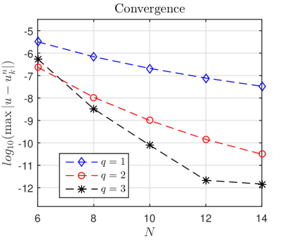
(a) $c=1.4$

(b) $c=0.5$

Figure 1: Convergence of scheme (4.5) for different $c$ with $\gamma=0.8$, $M=10000$.

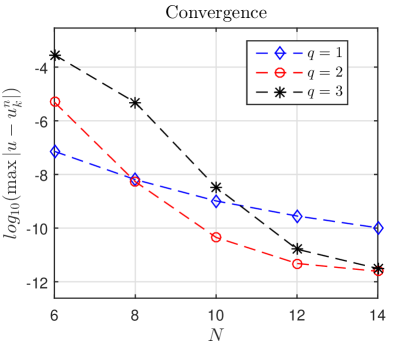
Figure 2: Convergence of scheme (4.5) with $c=3.1$, $\gamma=0.5$, $M=10000$.

Maximum errors for different $N$ are shown in Figure 1 with $c=1.4$, $\gamma=0.8$ and $c=0.5,\gamma=0.8$ separately. The Figure 2 displays that the convergence rate increases as $q$ increases. The results shown in these figures, along with the results in Table 5, suggest that it is profitable to perform smooth transformation on the equation no matter what regularity the solution has.

Example 5.2.

In this example, we consider equation (1.2) with $X=1,T=1$, and

$$\left\{\begin{aligned} &u(x,0)=0,\\ &u(0,t)=0,\quad u(1,t)=0,\\ &f(x,t)=\left(k_{\gamma}t^{c}+\pi^{2}t^{c+\gamma}\right)\sin\pi x,\end{aligned}\right.$$ (5.2)

where $k_{\gamma}=\frac{\Gamma(c+\gamma+1)}{\Gamma(c+1)}$ and $K_{\gamma}=1$. The exact solution of equation (1.2) is

$$u(x,t)=t^{c+\gamma}\sin\pi x.$$

It is also the solution of equation in the following form:

$$\left\{\begin{aligned} &\prescript{RL}{0}{\mathcal{D}}^{\gamma}_{T}u=u_{xx}+f\\ &u(x,0)=0,u(t,0)=0,u(t,1)=0,\\ &f=k_{\gamma}t^{c}\sin\pi x+\pi^{2}t^{c+\gamma}\sin\pi x,\end{aligned}\right.$$ (5.3)

This equation is equivalent with our equation (1.2). In [21], the authors solved these sub-diffusion equations with this form. Here, we compare the numerical results of scheme (4.12) with the results of the method developed by Zheng et al. in [21], which possesses high efficiency and exponential decay in both time and space directions.

Table 6: Maximum errors of scheme (4.12) with $c=2.5$, $\gamma=0.4$, $M^{\prime}=200$

$N$	6	8	10	12	14
$q=1$	4.87e-07	6.38e-08	1.26e-08	3.23e-09	1.00e-09
$q=2$	5.31e-07	7.01e-09	1.80e-10	7.27e-12	4.90e-13
$q=3$	7.60e-05	8.67e-08	7.51e-10	1.56e-11	3.13e-13
Zheng et al.	6.66e-06	9.98e-07	2.26e-07	6.62e-08	2.32e-08

Table 7: Maximum errors of scheme (4.12) with $c=1.5$, $\gamma=0.4$, $M^{\prime}=200$

$N$	6	8	10	12	14
$q=1$	2.25e-06	5.10e-07	1.54e-07	5.58e-08	2.32e-08
$q=2$	2.39e-07	7.95e-09	4.85e-10	5.31e-11	8.67e-12
$q=3$	8.45e-07	1.28e-08	3.80e-10	2.61e-11	1.17e-12
Zheng et al.	3.60e-05	9.63e-06	3.38e-06	1.41e-06	6.67e-07

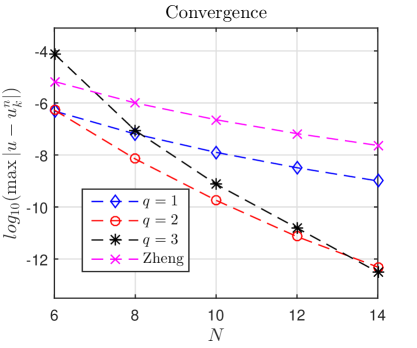
(a) $c=2.5$

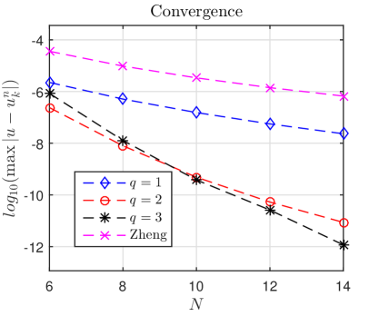
(b) $c=1.5$

Figure 3: Convergence of scheme (4.12) for different $c$ with $\gamma=0.4$, $M^{\prime}=200$.

In this example we take $\gamma=0.4$ and use the polynomials degree of spatial base $M^{\prime}=200$ to calculate results with different $c$. First, we choose $c=2.5,1.5$, and present the maximum errors in Table 6 and Table 7 respectively. In addition to visualize these data, we plot them in Figure 3. From those tables and figures, we can see that Zheng’s result is close to our result with $q=1$, and larger $q$ can significantly improve the accuracy. Also, notice that larger $q$ can speed up the convergence.

Table 8: Maximum errors of scheme (4.12) with $c=0.5$, $\gamma=0.4$, $M^{\prime}=200$

$N$	10	18	26	34	42	50
$q=1$	4.38e-06	4.64e-07	1.04e-07	3.39e-08	1.40e-08	6.76e-09
$q=2$	1.27e-08	1.42e-10	7.00e-12	7.23e-13	1.19e-13	2.18e-14
$q=3$	4.31e-09	1.51e-11	3.63e-13	2.32e-14	1.11e-15	1.22e-15
Zheng et al.	1.48e-04	2.56e-05	8.09e-06	3.42e-06	1.72e-06	9.68e-07

Table 9: Maximum errors of scheme (4.12) with $c=-0.1$, $\gamma=0.4$, $M^{\prime}=200$

$N$	10	18	26	34	42	50
$q=1$	1.95e-05	4.14e-06	1.50e-06	7.15e-07	4.05e-07	2.57e-07
$q=2$	1.47e-06	9.93e-08	1.68e-08	4.50e-09	1.58e-09	6.71e-10
$q=3$	1.57e-07	3.65e-09	3.22e-10	5.32e-11	1.27e-11	3.83e-12

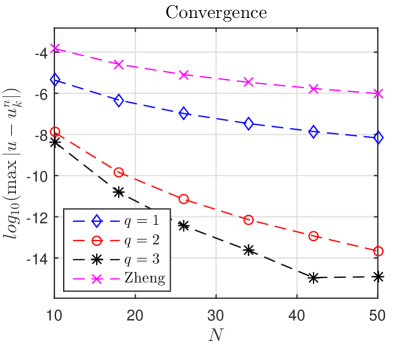
(a) $c=0.5$

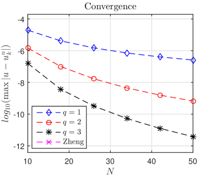
(b) $c=-0.1$

Figure 4: Convergence of scheme (4.12) for different $c$ with $\gamma=0.4$, $M^{\prime}=200$.

Furthermore, we choose $c=0.5,-0.1$, and present the results in Table 8, Table 9, and Figure 4. Zheng’s method cannot handle the situation with $c=-0.1$ and hence we just present our result in table and figure when $c=-0.1$. As $c$ decreases, the regularity of the solution becomes weaker, and this results in slow convergence speed as shown in Figure 3 and Figure 4. However, we can still get accurate results by setting $q$ larger. It is recommended to apply smooth transformation on the equations.

Example 5.3.

Consider anomalous sub-diffusion equation

$$\frac{\partial u}{\partial t}=\frac{\partial^{1-\gamma}}{\partial t^{1-\gamma}}\Big{(}\frac{\partial^{2}u}{\partial x^{2}}\Big{)},$$ (5.4)

with initial and boundary conditions [22]

$$u(x,0)=\left\{\begin{aligned} &2x,&0\leq x\leq 0.5,\\ &\frac{4-2x}{3},&0.5\leq x\leq 2,\end{aligned}\right.$$ (5.5)

$$u(0,t)=u(2,t)=0,\quad 0\leq t\leq 0.4\,.$$

This system is simulated by applying scheme (4.5) with $N=20,M=20$. Figure 5 shows the numerical approximation $u(x,t)$ when $\gamma=0.1$ and $\gamma=0.9$ respectively. And Figure 6 illustrates the change of approximation $u(x,t)$ as $\gamma$ vary in quantity. These results show that the system exhibits sub-diffusion behaviors and the solution continuously depends on the time fractional derivative.

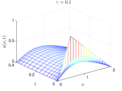
(a) $\gamma=0.1$

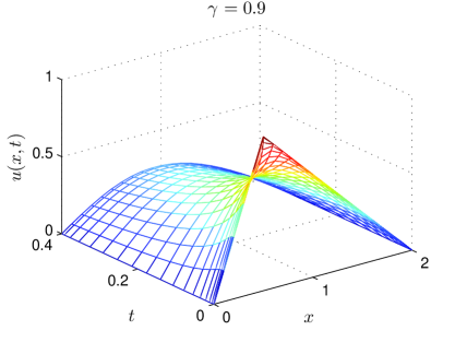
(b) $\gamma=0.9$

Figure 5: Numerical approximation of $u(x,t)$ for different $\gamma$ when $N=20,M=20$.

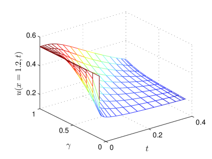
(a) $x=1.2$

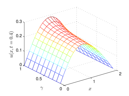
(b) $t=0.4$

Figure 6: The numerical approximation $u(x,t)$ for various $\gamma$ when $N=20,M=20$.

6 Conclusion

In this paper, a high-order method has been proposed to solve anomalous sub-diffusion equations especially when the exact solution has lower regularity. The compact difference method and the spectral method used in spatial direction make this method more effective. In the numerical experiments, we have demonstrated the effectiveness and accuracy of these proposed schemes, even though theoretical analysis of convergence order and stability for this method are lacked because of the difficulty of coupled integral and differential operator. In the future, we will focus on the theoretical analysis of this method.

References

- [1] P. Baratella and A. Palamara Orsi. A new approach to the numerical solution of weakly singular Volterra integral equations. J. Comput. Appl. Math., 163(2):401–418, 2004.
- [2] A. Cartea and D. del Castillo-Negrete. Fluid limit of the continuous-time random walk with general Lévy jump distribution functions. Phys. Rev. E, 76:041105, 2007.
- [3] M. Dehghan, J. Manafian and A. Saadatmandi. Solving nonlinear fractional partial differential equations using the homotopy analysis method. Numer. Methods Partial Differential Equations, 26(2):448–479, 2010.
- [4] M. Dehghan, M. Safarpoor and M. Abbaszadeh. Two high-order numerical algorithms for solving the multi-term time fractional diffusion-wave equations. J. Comput. Appl. Math., 290:174–195, 2015.
- [5] M. Dehghan and M. Safarpoor. The dual reciprocity boundary integral equation technique to solve a class of the linear and nonlinear fractional partial differential equations. Math. Meth. Appl. Sci., 39:2461–2476, 2015.
- [6] M. Dehghan, M. Abbaszadeh and A. Mohebbi. Legendre spectral element method for solving time fractional modified anomalous sub-diffusion equation. Appl. Math. Model., 40(5):3635–3654, 2016.
- [7] M. Dehghan and M. Abbaszadeh. Spectral element technique for nonlinear fractional evolution equation, stability and convergence analysis. Appl. Numer. Math., 119:51–66, 2017.
- [8] G. H. Gao, H. W. Sun, and Z. Z. Sun. Stability and convergence of finite difference schemes for a class of time-fractional sub-diffusion equations based on certain superconvergence. J. Comput. Phys., 280:510–528, 2015.
- [9] G. H. Gao and Z. Z. Sun. A compact finite difference scheme for the fractional sub-diffusion equations. J. Comput. Phys., 230(3):586–595, 2011.
- [10] R. Gorenflo, F. Mainardi, E. Scalas, and M. Raberto. Mathematical Finance: Workshop of the Mathematical Finance Research Project, Konstanz, Germany, October 5–7, 2000, chapter Fractional Calculus and Continuous-Time Finance III : the Diffusion Limit, pages 171–180. Birkhäuser Basel, Basel, 2001.
- [11] R. L. Magin. Fractional calculus models of complex dynamics in biological tissues. Comput. Math. Appl., 59(5):1586–1593, 2010.
- [12] R. Metzler and J. Klafter. The random walk’s guide to anomalous diffusion: a fractional dynamics approach. Phys. Rep., 339(1):1–77, 2000.
- [13] G. Monegato and I. H. Sloan. Numerical solution of the generalized airfoil equation for an airfoil with a flap. SIAM J. Numer. Anal., 34(6):2288–2305, 1997.
- [14] K. Mustapha, B. Abdallah and K. M. Furati A Discontinuous Petrov–Galerkin Method for Time-Fractional Diffusion Equations. SIAM J. Numer. Anal., 52(5):2512–2529, 2014.
- [15] K. Mustapha. Time-stepping discontinuous Galerkin methods for fractional diffusion problems. Numer. Math., 130(3):497–516, 2015.
- [16] J. Shen, T. Tang, and L.-L. Wang. Spectral Mehtods: Algorithms, Analysis and Applications. Number 41 in Springer Series in Computational Mathematics. Springer-Verlag Berlin Heidelberg, first edition, 2011.
- [17] S. B. Yuste and L. Acedo. An explicit finite difference method and a new von neumann-type stability analysis for fractional diffusion equations. SIAM J. Numer. Anal., 42(5):1862–1874, 2005.
- [18] S. B. Yuste and L. Acedo. Some exact results for the trapping of subdiffusive particles in one dimension. Phys. A, 336(3-4):334–346, 2004.
- [19] G. M. Zaslavsky. Chaos, fractional kinetics, and anomalous transport. Phys. Rep., 371:461–580, December 2002.
- [20] F. Zeng, C. Li, F. Liu, and I. Turner. The use of finite difference/element approaches for solving the time-fractional subdiffusion equation. SIAM J. Sci. Comput., 35(6):A2976–A3000, 2013.
- [21] M. Zheng, F. Liu, V. Anh, and I. Turner. A high-order spectral method for the multi-term time-fractional diffusion equations. Appl. Math. Model., 40(7-8):4970–4985, 2015.
- [22] P. Zhuang, F. Liu, V. Anh, and I. Turner. New solution and analytical techniques of the implicit numerical method for the anomalous subdiffusion equation. SIAM J. Numer. Anal., 46(2):1079–1095, 2008.