Joint Learning of Siamese CNNs and Temporally Constrained Metrics for Tracklet Association

Abstract

In this paper, we study the challenging problem of multi-object tracking in a complex scene captured by a single camera. Different from the existing tracklet association-based tracking methods, we propose a novel and efficient way to obtain discriminative appearance-based tracklet affinity models. Our proposed method jointly learns the convolutional neural networks (CNNs) and temporally constrained metrics. In our method, a Siamese convolutional neural network (CNN) is first pre-trained on the auxiliary data. Then the Siamese CNN and temporally constrained metrics are jointly learned online to construct the appearance-based tracklet affinity models. The proposed method can jointly learn the hierarchical deep features and temporally constrained segment-wise metrics under a unified framework. For reliable association between tracklets, a novel loss function incorporating temporally constrained multi-task learning mechanism is proposed. By employing the proposed method, tracklet association can be accomplished even in challenging situations. Moreover, a new dataset with 40 fully annotated sequences is created to facilitate the tracking evaluation. Experimental results on five public datasets and the new large-scale dataset show that our method outperforms several state-of-the-art approaches in multi-object tracking.

I Introduction

Multi-object tracking in real scenes is an important topic in computer vision, due to its demands in many essential applications such as surveillance, robotics, traffic safety and entertainment. As the seminal achievements were obtained in object detection [1, 2, 3], tracklet association-based tracking methods [4, 5, 6, 7, 8] have become popular recently. These methods usually include two key components: 1) A tracklet affinity model that estimates the linking probability between tracklets (track fragments), which is usually based on the combination of multiple cues (motion and appearance cues); 2) A global optimization framework for tracklet association, which is usually formulated as a maximum a posterior problem (MAP).

Even though some state-of-the-art methods [4, 6, 9] have achieved much progress in constructing discriminative appearance and motion based tracklet affinity models, problems such as track fragmentation and identity switch still cannot be well handled, especially under difficult situations where the appearance or motion of an object changes abruptly and significantly. Some of state-of-the-art tracklet association-based multi-object tracking methods [4, 9] make use of image representations which are not well-suited for constructing robust appearance-based tracklet affinity models. These methods usually utilize pre-selected features, such as HOG features [1], local binary patterns [2], or color histograms, which are not “tailor-made” for the tracked objects in question. Recently, deep convolutional neural network architectures have been successfully applied to many challenging tasks, such as image classification [10] and object detection [11], and been reported highly promising results. The core to the deep convolutional neural network’s success is to take the advantage of deep architectures to learn richer hierarchical features through multiple nonlinear transformations. Hence, we adopt the deep convolutional neural network for multi-object tracking in this work.

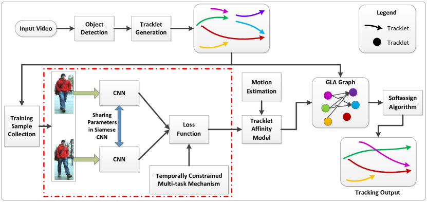
Figure 1: Tracking framework of our method. In the Generalized Linear Assignment (GLA) [12] graph, each node denotes a reliable tracklet; each edge denotes a possible link between two tracklets. Our method jointly learns the parameters of the Siamese CNN and the temporally constrained metrics for tracklet affinity model, as shown in the red-dashed box, which estimates the linking probability between two tracklets in the GLA graph. The tracking results are obtained by combinatorial optimization using the softassign algorithm [13].

Traditional deep neural networks [10, 14] are designed for the classification task. Here, we aim to associate tracklets by joint learning of the convolutional neural networks and the appearance-based tracklet affinity models. This joint optimization will maximize their capacity for solving tracklet association problems. Hence, we propose to jointly learn the Siamese convolutional neural network, which consists of two sub-networks (see Figure 1), and appearance-based tracklet affinity models, so that the appearance-based affinity models and the “tailor-made” hierarchical features for tracked targets are learned simultaneously and coherently. Furthermore, based on the analysis of the characteristics of the sequential data stream, a novel temporally constrained multi-task learning mechanism is proposed to be added to the objective function. This makes the deep architectures more effective in tackling the tracklet association problem. Although deep architectures have been employed in single object tracking [15, 16, 17, 18, 19], we explore deep architectures for multi-object tracking in this work.

The proposed framework in this paper is shown in Figure 1. Given a video input, we first detect objects in each frame by a pre-trained object detector, such as the popular DPM detector [3]. Then a dual-threshold strategy [20] is employed to generate reliable tracklets. The Siamese CNN is first pre-trained on the auxiliary data offline. Subsequently, the Siamese CNN and temporally constrained metrics are jointly learned online for tracklet affinity models by using the online collected training samples among the reliable tracklets. Finally, the tracklet association problem is formulated as a Generalized Linear Assignment (GLA) problem, which is solved by the softassign algorithm [13]. The final trajectories of multiple objects are obtained after a trajectory recovery process.

The contributions of this paper can be summarized as: (1) We propose a unified deep model for jointly learning “tailor-made” hierarchical features for currently tracked objects and temporally constrained segment-wise metrics for tracklet affinity models. With this deep model, the feature learning and the discriminative tracklet affinity model learning can efficiently interact with each other, maximizing their performance co-operatively. (2) A novel temporally constrained multi-task learning mechanism is proposed to be embedded into the last layer of the unified deep neural network, which makes it more effective to learn appearance-based affinity model for tracklet association. (3) A new large-scale dataset with 40 diverse fully annotated sequences is built to facilitate performance evaluation. This new dataset includes 24,882 frames and 246,330 annotated bounding boxes of pedestrians.

The remainder of this paper is organized as follows: The unified deep model is introduced in Section II. Section III describes the tracklet association framework. The new large-scale dataset and experimental results are introduced in Section IV. Section V concludes the paper.

II The Unified Deep Model

In this section, we explain how the unified deep model is designed for jointly learning hierarchical features and temporally constrained metrics for tracklet association.

II-A The Architecture

A deep neural network usually works in a standalone mode for most of computer vision tasks, such as image classification, object recognition and detection. The input and output of the deep neural network in this mode are a sample and a predicted label respectively. However, for the tracklet association problem, the objective is to estimate the tracklet affinities between two tracklets to decide whether they belong to the same object. Hence, the “sample $\rightarrow$ label” mode deep neural network is not applicable to the tracklet association problem. To deal with this problem, we propose to create a Siamese deep neural network, which consists of two sub-networks working in a “sample pair $\rightarrow$ similarity” mode.

The structure of the Siamese convolution neural network (CNN) is shown in Figure 1 (red-dashed box). Given two target images, they are first warped to a fixed 96 $\times$ 96 patch and presented to the Siamese CNN. The Siamese CNN is composed of two sub convolutional neural networks (CNNs), as shown in Figure 1 (red-dashed box). A novel metric learning based loss function is proposed for learning this Siamese CNN. Moreover, the Siamese CNN has their two sub-CNNs sharing the same parameters, i.e., weights and biases.

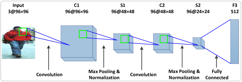
Figure 2: The structure of 5-layer sub-CNN used in the unified deep model.

The sub-CNN in the unified deep model consists of 2 convolutional layers (C1 and C2), 2 max pooling layers (S1 and S2) and a fully connected layer (F3), as shown in Figure 2. The number of channels of convolutional and max pooling layers are both 96. The output of the sub-CNN is a feature vector of 512 dimensions. A cross-channel normalization unit is included in each pooling layer. The convolutional layer output has the same size as the input by zero padding of the input data. The filter sizes of C1 and C2 layers are 7 $\times$ 7 and 5 $\times$ 5 respectively. The activation function for each layer in the CNN is ReLU neuron [10].

II-B Loss Function and Temporally Constrained Metric Learning

As we can see in Figure 1 (red-dashed box), the Siamese CNN consists of two basic components: two sub-CNNs and a loss function. The loss function converts the difference between the paired input samples into a margin-based loss.

The relative distance between an input sample pair used in the loss function, parameterized as a Mahalanobis distance, is defined as:

$${{\|x_{i}-x_{j}\|}_{M}}^{2}={(x_{i}-x_{j})}^{T}M(x_{i}-x_{j}),\quad i\neq j$$ (1)

where $x_{i}$ and $x_{j}$ are two 512-dimensional feature vectors obtained from the last layer of the two sub-CNNs; and $M$ is a positive semidefinite matrix.

Before introducing the proposed loss function with the temporally constrained multi-task learning mechanism, we first present the loss function with common metric learning. Given training samples, we aim to minimize the following loss:

$$\min_{M}\frac{\lambda}{2}{{\|M-I\|}_{F}}^{2}+C\sum_{i,j}\max(0,b-l_{i,j}[1-{{\|x_{i}-x_{j}\|}_{M}}^{2}])$$

$$s.t.\quad M\succeq 0,i\neq j$$ (2)

where $\lambda$ is a regularization parameter; ${\|\cdot\|}_{F}$ denotes the Frobenius norm of a matrix; $C$ is the weight parameter of the empirical loss; $b$ is a constant value satisfying $0\leq b\leq 1$, which represents the decision margin; $l_{i,j}$ is a label that equals to 1 when $x_{i}$ and $x_{j}$ are of the same object and -1 otherwise; and $M\succeq 0$ means that $M$ is a positive semidefinite matrix.

Nevertheless, object appearance can vary a lot in the entire video sequence. It is undesirable to use the same metric to estimate the tracklet affinities over the entire video sequence. In this paper, segment-wise metrics are proposed to be learned within each short-time segment, known as local segment. Meanwhile, to capture the common discriminative information shared by all the segments, a multi-task learning mechanism is proposed to be embedded into the loss function for learning the segment-wise and common metrics simultaneously. Moreover, segments in videos are temporal sequences. Temporally close segments should share more information. Hence, we propose a multi-task learning method incorporating temporal constraints for this learning problem:

$$\min_{M_{0},...,M_{n}} \bigg{(}\frac{\lambda_{0}}{2}{{\|M_{0}-I\|}_{F}}^{2}+\sum_{t=2}^{n}\frac{\eta}{2}{{\|M_{t}-M_{t-1}\|}_{F}}^{2}+$$

$$\sum_{t=1}^{n}[\frac{\lambda}{2}{{\|M_{t}\|}_{F}}^{2}+C\sum_{i,j}h(x_{i},x_{j})]\bigg{)}$$

$$s.t.\quad M_{0},M_{1},...,M_{n}\succeq 0,i\neq j$$ (3)

where $\lambda_{0}$ and $\lambda$ are the regularization parameters of $M_{t}$ for $t=0,1,...,n$; $n$ is the total number of segments; $M_{0}$ is the common metric shared by all the segments; $M_{t}$ is the segment-wise metric; ${\|\cdot\|}_{F}$ denotes the Frobenius norm of a matrix; the second term of this loss function is the temporal constraint term, in which $\eta$ is a regularization parameter; $h(x_{i},x_{j})$ is the empirical loss function; and $C$ is the weight parameter of the empirical loss.

The empirical loss function $h(x_{i},x_{j})$ used in Equation (3) is expressed as:

$$h(x_{i},x_{j})=\max(0,b-l_{i,j}[1-{{\|x_{i}-x_{j}\|}_{M_{tot}}}^{2}]);$$ (4)

$$M_{tot}=M_{0}+M_{t},\quad i\neq j,$$

$${{\|x_{i}-x_{j}\|}_{M_{tot}}}^{2}={(x_{i}-x_{j})}^{T}(M_{0}+M_{t})(x_{i}-x_{j})$$

where $b$ is a constant value, which represents the decision margin; $l_{i,j}$ is a label that equals to 1 when $x_{i}$ and $x_{j}$ are of the same object and -1 otherwise; $x_{i}$ and $x_{j}$ are two 512-dimensional feature vectors obtained from the last layer of the two sub-CNNs; and $M_{tot}$ is the metric used for estimating the relative distance between a sample pair.

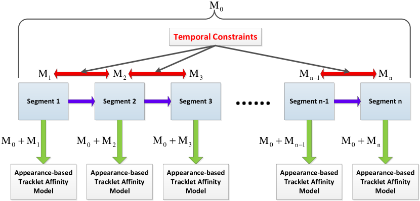
Figure 3: An illustration of the temporally constrained multi-task learning mechanism. $n$ is the total number of the segments and the segments are shown in the temporal space.

Intuitively, the common metric $M_{0}$ represents the shared discriminative information across the entire video sequence and the segment-wise metric $M_{t>0}$ adapt the metric for each local segment. In the proposed objective function, in Equation (3), the second term is the temporal constraint term, which accounts for the observation that the neighboring segments sharing more information than the non-neighboring segments (see Figure 3 for an illustration). In the implementation, we use the previous segment-wise metric $M_{t-1}$ in temporal space to initialize the current segment-wise metric $M_{t}$, due to the assumption that the neighboring segment-wise metrics are more correlated than the non-neighboring ones.

To learn the parameters of the unified deep model, back-propagation (BP) [21] is utilized. The forward propagation function to calculate the loss of the training pairs is presented in Equation (3). By differentiating the loss function with respect to the two input samples, we have the gradients. The total gradient for back-propagation is the sum of the contributions from the two samples, which is as follows:

$$\nabla G_{total}=2Cl_{i,j}(M_{tot}+{M_{tot}}^{T})(x_{i}-x_{j})\left(\mathbbm{I}\{g(x_{i},x_{j})>0\}\right)$$ (5)

where

$$M_{tot}=M_{0}+M_{t},$$ (6)

$$g(x_{i},x_{j})=b-l_{i,j}[1-{{\|x_{i}-x_{j}\|}_{M_{tot}}}^{2}],$$ (7)

$${{\|x_{i}-x_{j}\|}_{M_{tot}}}^{2}={(x_{i}-x_{j})}^{T}(M_{0}+M_{t})(x_{i}-x_{j})$$ (8)

and $\mathbbm{I}\{\cdot\}$ is the indicator function.

Based on Equations (3) and (5), we can learn the parameters of the unified deep model by stochastic gradient descent [10] via back-propagation. Moreover, the temporally constrained metrics for tracklet affinity models are obtained simultaneously by batch mode stochastic gradient descent. By differentiating the loss function, as shown in Equation (3), with respect to the common metric $M_{0}$ and the segment-wise metric $M_{t>0}$, the gradients are:

$$\nabla G_{0} =\frac{\partial L}{\partial M_{0}}$$

$$=\lambda_{0}(M_{0}-I)+C\sum_{i,j}l_{i,j}A_{i,j}\left(\mathbbm{I}\{g(x_{i},x_{j})>0\}\right);$$ (9)

$$\nabla G_{t} =\frac{\partial L}{\partial M_{t}}$$

$$=\left\{\begin{array}[]{ll}\lambda M_{t}+C\sum_{i,j}l_{i,j}A_{i,j}\left(\mathbbm{I}\{g(x_{i},x_{j})>0\}\right),\\ \quad\quad\quad\quad\quad\quad\quad\quad\quad\quad\text{if}\ \ t=1;\\ \\ \Big{(}\eta(M_{t}-M_{t-1})+\lambda M_{t}+\\ C\sum_{i,j}l_{i,j}A_{i,j}\left(\mathbbm{I}\{g(x_{i},x_{j})>0\}\right)\Big{)},\\ \quad\quad\quad\quad\quad\quad\quad\quad\quad\quad\text{otherwise}\ (t>1).\end{array}\right.$$ (16)

where

$$A_{i,j}=(x_{i}-x_{j})(x_{i}-x_{j})^{T},$$ (17)

$$g(x_{i},x_{j})=b-l_{i,j}[1-{{\|x_{i}-x_{j}\|}_{M_{tot}}}^{2}],$$ (18)

$${{\|x_{i}-x_{j}\|}_{M_{tot}}}^{2}={(x_{i}-x_{j})}^{T}(M_{0}+M_{t})(x_{i}-x_{j})$$ (19)

Online training sample collection is an important issue in the learning of the unified deep model. We take the assumptions similar to those as in [4]: (1) detection responses in one tracklet are from the same object; (2) any detection responses in two different tracklets which have overlaps over time are from different objects. The first one is based on the assumption that the tracklets generated by the dual-threshold strategy are reliable; the second one is based on the fact that one target cannot appear at two or more different locations at the same time, known as spatio-temporal conflict. For each tracklet, $\kappa$ strongest detection responses are selected as training samples ($\kappa=4$ in our implementation). Then we use two arbitrarily selected different detection responses from the $\kappa$ strongest responses of $T_{i}$ as positive training samples, and two detection responses from the $\kappa$ strongest responses of two spatio-temporal conflicted tracklets as negative training samples.

Finally, the common metric $M_{0}$ and the segment-wise metrics $M_{t>0}$ are obtained simultaneously through a gradient descent rule. The online learning algorithm is summarized in Algorithm 1.

$$M_{0}= M_{0}-\beta\frac{\partial L}{\partial M_{0}}$$ (20)

$$M_{t}= M_{t}-\beta\frac{\partial L}{\partial M_{t}}$$ (21)

where $\beta$ is the learning rate.

Meanwhile, the Siamese CNN is online fine-tuned through back propagating the gradients calculated by Equation (5).

Algorithm 1 Online Learning Algorithm for Temporally Constrained Metric Learning

0:     Feature vectors of online collected training samples $\{{x_{i}}^{t}\}$; $i=1,...,n_{t}$, $n_{t}$ is the number of the samples within segment $t$; $t=1,...,n$, $n$ is the total number of the segments; and learning rate $\beta$.

0:     The learned metrics: $M_{0},M_{1},...,M_{n}$.

1:  Initialize $M_{0}=I$ (identity matrix).

2:  for $t=1,...,n$ do

3:     if $t==1$ then

4:        Initialize $M_{t}=0$.

5:     else

6:        Initialize $M_{t}=M_{t-1}$.

7:     end if

8:     Randomly generate the training pairs $\{x_{i},x_{j},l_{i,j}\}$ from $\{{x_{i}}^{t}\}$. $l_{i,j}=1$, if $x_{i}$ and $x_{j}$ are from one tracklet; $l_{i,j}=-1$, if $x_{i}$ and $x_{j}$ are from two different tracklets which have overlaps over time. A total of $2m$ training pairs in a random order are generated, which includes $m$ positive and $m$ negative pairs.

9:     for $p=1,...,2m$ do

10:        if $l_{i,j}[1-{(x_{i}-x_{j})}^{T}(M_{0}+M_{t})(x_{i}-x_{j})]>b$ then

11:           $M_{0}$=$M_{0}$; $M_{t}$=$M_{t}$.

12:        else if $l_{i,j}<0$ then

13:           Compute $M_{0}$ and $M_{t}$ by Equations (20) and (21).

14:        else

15:           $M_{0}=\pi_{S+}(M_{0}-\beta\frac{\partial L}{\partial M_{0}})$;

16:           $M_{t}=\pi_{S+}(M_{t}-\beta\frac{\partial L}{\partial M_{t}})$; where $\pi_{S+}(A)$ projects matrix $A$ into the positive semidefinite cone.

17:        end if

18:     end for

19:  end for

III Tracklet Association Framework

In this section, we present the tracklet association framework, in which, we incorporate the temporally constrained metrics learned by the unified deep model to obtain robust appearance-based tracklet affinity models.

III-A Tracklet Association with Generalized Linear Assignment

To avoid learning tracklet starting and termination probabilities, we formulate the tracklet association problem as a Generalized Linear Assignment (GLA) [12], which does not need the source and sink nodes as in conventional network flow optimization [22, 23, 24, 8]. Given $N$ tracklets $\{T_{1},...,T_{N}\}$, the Generalized Linear Assignment (GLA) problem is formulated as:

$$\max_{X}\sum_{i=1}^{N}\sum_{j=1}^{N}P(T_{i},T_{j})X_{ij}$$ (22)

$$s.t.\quad\sum_{i=1}^{N}X_{ij}\leq 1;\sum_{j=1}^{N}X_{ij}\leq 1;X_{ij}\in\{0,1\}$$

where $P(T_{i},T_{j})$ is the linking probability between $T_{i}$ and $T_{j}$. The variable $X_{ij}$ denotes that $T_{i}$ is the predecessor of $T_{j}$ in temporal domain when $X_{ij}=1$ and that, they may be merged during the optimization.

III-B Tracklet Affinity Measurement

To solve the Generalized Linear Assignment (GLA) problem in Equation (22), we need to estimate the tracklet affinity score, or equivalently, the linking probability, $P(T_{i},T_{j})$, between two tracklets. The linking probability $P(T_{i},T_{j})$ is defined based on two cues: motion and appearance.

$$P(T_{i},T_{j})=P_{m}(T_{i},T_{j})P_{a}(T_{i},T_{j})$$ (23)

The motion-based tracklet affinity model $P_{m}(T_{i},T_{j})$ is defined as:

$$P_{m}(T_{i},T_{j})= \mathcal{N}(p_{i}^{tail}+v_{i}^{F}\Delta t;p_{j}^{head},\Sigma)\cdot$$

$$\mathcal{N}(p_{j}^{head}+v_{j}^{B}\Delta t;p_{i}^{tail},\Sigma)$$ (24)

where $p_{i}^{tail}$ is the position of the tail response in $T_{i}$; $p_{j}^{head}$ is the position of the head response in $T_{j}$; $v_{i}^{F}$ is the forward velocity of $T_{i}$; $v_{j}^{B}$ is the backward velocity of $T_{j}$; and $\Delta t$ is the time gap between the tail response of $T_{i}$ and the head response of $T_{j}$.

In Equation (24), the forward velocity $v_{i}^{F}$ is estimated from the head to the tail of $T_{i}$, while the backward velocity $v_{j}^{B}$ is estimated from the tail to the head of $T_{j}$. It is assumed that the difference of the predicted position and the refined position follows a Gaussian distribution.

To estimate the appearance-based tracklet affinity scores, we need to construct the probe set, consisting of the strongest detection response in each tracklet. The probe set is defined as $G=\{g_{i}\}$, $i=1,...,N_{s}$, in which $N_{s}$ is the number of tracklets in a local segment. Each $T_{i}$ has only one selected $g_{i}$ in $G$ to represent itself.

The appearance-based tracklet affinity model $P_{a}(T_{i},T_{j})$ is defined based on the learned temporally constrained metrics:

$$d_{ij}^{k}=(x_{i}^{k}-g_{j})^{T}(M_{0}+M_{t})(x_{i}^{k}-g_{j});$$

$$d_{ji}^{k^{\prime}}=(x_{j}^{k^{\prime}}-g_{i})^{T}(M_{0}+M_{t})(x_{j}^{k^{\prime}}-g_{i});$$

$$norm_{i}^{k}=\sqrt{(\sum_{j=1}^{N_{s}}d_{ij}^{k})};\ norm_{j}^{k^{\prime}}=\sqrt{(\sum_{i=1}^{N_{s}}d_{ji}^{k^{\prime}})};$$

$$d_{ij}=\Big{[}\sum_{k}(\frac{d_{ij}^{k}}{norm_{i}^{k}})\Big{]}/m_{i};\ d_{ji}=\Big{[}\sum_{k^{\prime}}\frac{d_{ji}^{k^{\prime}}}{norm_{j}^{k^{\prime}}}\Big{]}/m_{j};$$

$$P_{a}(T_{i},T_{j})=(d_{ij}d_{ji})^{-1}$$ (25)

where $x_{i}^{k}$ denotes the feature vector of the $k$th detection response in $T_{i}$; $x_{j}^{k^{\prime}}$ denotes the feature vector of the $k^{\prime}$th detection response in $T_{j}$; $g_{i},g_{j}\in G$; $m_{i}$ and $m_{j}$ are the numbers of detection responses of $T_{i}$ and $T_{j}$ respectively.

Through Equation (23), we can obtain the predecessor-successor matrix $P$ for the objective function (22). To achieve fast and accurate convergence, $P$ is normalized by column and a threshold $\omega$ is introduced to ensure that a reliable tracklet association pair has a high affinity score.

$$P(T_{i},T_{j})=\left\{\begin{array}[]{lll}P_{m}(T_{i},T_{j})P_{a}(T_{i},T_{j}),\\ \quad\ if\ P_{m}(T_{i},T_{j})P_{a}(T_{i},T_{j})\geq\omega\\ \\ 0,\ \text{otherwise}\\ \end{array}\right.$$ (30)

The Generalized Linear Assignment problem in Equation (22) can be solved by the softassign algorithm [13]. Due to missed detections, there may exist some gaps between adjacent tracklets in each trajectory after tracklet association. Therefore, the final tracking results are obtained through a trajectory interpolation process over gaps based on a linear motion model.

IV Experiments

IV-A Datasets

IV-A1 Public Datasets

To evaluate the multi-object tracking performance of the proposed method, experiments are conducted on five publicly available datasets: PETS 2009 [25], Town Centre [26], Parking Lot [27], ETH Mobile scene [28] and MOTChallenge [29].

IV-A2 New Large-Scale Dataset

As generally known, a representative dataset is a key component in comprehensive performance evaluation. In recent years, several public datasets have been published for multi-target tracking, such as TUD [30], Town Centre[26], ParkingLot[27], ETH[28] and PETS[25]. Nevertheless, for most of the public datasets, the number of testing sequences is limited. The sequences usually lack sufficient diversity, which makes the tracking evaluation short of desired comprehensiveness. Recently, the KITTI benchmark [31] was developed via autonomous driving platform for computer vision challenges, which includes stereo, optical flow, visual odometry, object detection and tracking. However, in this benchmark, the camera is only put on the top of a car for all sequences, resulting in less diversity. Moreover, an up-to-date MOTChallenge benchmark [29] was very recently made available for multi-target tracking. Compared with other datasets, this MOTChallenge [29] is a more comprehensive dataset for multi-target tracking. However, there are still some limitations for this MOTChallenge benchmark. First, 18 testing sequences are included, which are still insufficient to allow for a comprehensive evaluation for multi-target tracking. In the single object tracking area, researchers usually evaluate on more than 50 sequences [32] nowadays. Second, the testing sequences of MOTChallenge lack some specific scenarios such as pedestrians with uniforms. Furthermore, the pedestrian view, which is an important factor affecting the appearance models in multi-target tracking, is not analyzed in the MOTChallenge benchmark. Therefore, it is essential to create a more comprehensive dataset, which includes larger collection of sequences and covers more variations of scenarios, for multi-target tracking.

In this work, a new large-scale dataset containing 40 diverse fully annotated sequences is created to facilitate the evaluation. For this dataset, 10 sequences, which contain 5,080 fames and 52,833 annotated boxes of pedestrians, are used for training; 30 sequences, which contain 19,802 frames and 193,497 annotated boxes of pedestrians, are used for testing.

The new 40 sequences in this new large-scale dataset varies significantly from each other, which can be classified according to the following criteria: (1) Camera motion. The camera can be static like most surveillance cameras, or can be moving as held by a person or placed on a moving platform such as a stroller or a car. (2) Camera viewpoint. The scenes can be captured from a low position, a medium position (at pedestrian’s height), or a high position. (3) Weather conditions. Following the settings of MOTChallenge [29], the weather conditions are taken into consideration in this benchmark, which are sunny, cloudy and night. (4) Pedestrian view. The dominant pedestrian views in a sequence can be front view, side view or back view. For instance, if a sequence is taken in front of a group of pedestrians, moving towards the camera, the dominant pedestrian view of this sequence is front view. Moreover, the dominant pedestrian views in a sequence can have one, two or all of the views. If one sequence has more pedestrian views, it will be assigned into all the relevant categories. Table I and II show the overview of the training and testing sequences of the new dataset respectively. Figure 4 shows some examples of this new dataset. As shown in Figure 4, this new dataset contains the scenarios that pedestrians with uniforms.

IV-B Experimental Settings

Name	FPS	Resolution	Length	Tracks (in total)	Boxes of pedestrians	Density	Camera	Viewpoint	Weather	Front view	Side view	Back view
tokyo cross	25	640x480	700	24	6099	8.7	static	low	cloudy	yes	no	yes
paris cross	24	1920x1080	401	34	7319	18.3	static	low	cloudy	no	yes	no
london street	24	1920x1080	396	23	3758	9.5	static	low	cloudy	yes	no	yes
faneuil hall	25	1280x720	631	27	3928	6.2	moving	low	cloudy	yes	no	yes
central park	25	1280x720	600	39	4400	7.3	static	low	sunny	no	yes	no
long beach	24	1280x720	402	27	3599	9	moving	low	sunny	yes	no	no
oxford street	25	640x480	400	85	5807	14.5	moving	high	cloudy	yes	no	yes
sunset cross	24	1280x720	300	20	2683	8.9	static	high	sunny	yes	no	yes
rain street	25	640x480	800	30	10062	12.6	moving	low	cloudy	yes	yes	yes
USC campus	30	1280x720	450	37	5178	11.5	moving	low	sunny	yes	yes	yes
Total training			5080	346	52833

TABLE I: Overview of the training sequences included in the new dataset.

Name	FPS	Resolution	Length	Tracks (in total)	Boxes of pedestrians	Density	Camera	Viewpoint	Weather	Front view	Side view	Back view
book store	24	1280x720	905	78	8905	9.8	static	low	cloudy	no	yes	no
bronx road	24	1280x720	854	64	6623	7.8	moving	medium	sunny	yes	no	yes
child cross	30	1280x720	518	18	5389	10.4	static	medium	cloudy	yes	no	no
college graduation	30	1280x720	653	23	7410	11.3	moving	medium	cloudy	no	yes	yes
cuba street	25	1280x720	700	66	7518	10.7	moving	low	cloudy	yes	no	yes
footbridge	30	1280x720	678	21	3195	4.7	moving	low	sunny	yes	no	yes
india railway	50	1280x720	450	70	10799	24	static	high	sunny	yes	yes	yes
kuala lumpur airport	50	1280x720	1245	30	7732	6.2	moving	low	cloudy	yes	no	no
latin night	25	1280x720	700	23	5168	7.4	moving	low	night	yes	no	yes
london cross	30	640x480	740	30	4548	6.1	static	low	cloudy	yes	no	yes
london subway	30	1920x1080	361	31	2424	6.7	static	medium	cloudy	yes	yes	yes
london train	24	1920x1080	385	34	3207	8.3	static	low	cloudy	yes	no	yes
mexico night	30	640x480	1065	32	8164	7.7	static	low	night	yes	yes	yes
milan street	24	1280x720	293	40	4552	15.5	static	low	cloudy	yes	yes	yes
NYC subway gate	10	640x480	555	35	4578	8.2	static	low	cloudy	yes	no	yes
paris bridge	30	1920x1080	674	14	4506	6.7	static	medium	cloudy	no	yes	no
paris street	25	1280x720	300	35	3240	10.8	moving	medium	cloudy	yes	no	yes
pedestrian street	50	1280x720	1200	42	19799	16.5	static	low	sunny	yes	no	yes
phoenix park	24	1280x720	682	19	7655	11.2	static	low	sunny	yes	no	no
red light cross	30	640x480	300	16	2467	8.2	static	low	cloudy	yes	yes	no
regensburg bridge	25	1280x720	638	6	2967	4.7	static	low	sunny	yes	no	no
san franci walkstreet	25	1280x720	300	29	3659	12.2	static	low	cloudy	yes	yes	yes
shanghai overpass	24	1280x720	280	50	7940	28.4	static	low	cloudy	yes	yes	yes
shop corner	30	1280x720	900	43	10067	11.2	static	medium	cloudy	yes	yes	yes
stockholm1	25	1280x720	700	35	6077	8.7	moving	low	cloudy	yes	no	yes
tagbilaran airport	13	640x480	1026	39	6264	6.1	moving	high	sunny	yes	yes	no
taipei underpass	30	1280x720	300	26	2954	9.8	static	low	cloudy	yes	no	yes
tokyo park	25	1280x720	700	24	6034	8.6	moving	medium	sunny	yes	no	yes
tokyo shinkanzen	30	640x480	700	49	11297	16.1	moving	low	cloudy	yes	no	yes
tokyo street	25	1280x720	1000	29	8359	8.4	moving	low	sunny	yes	no	yes
Total testing			19802	1051	193497

TABLE II: Overview of the testing sequences included in the new dataset.

(a) India railway

(b) Oxford street

(c) College graduation

(d) Mexico night

Figure 4: Examples of the new large-scale dataset.

For the first four datasets evaluation, the proposed Siamese CNN is first pre-trained on the JELMOLI dataset [33] with the loss function in Equation (2). For the MOTChallenge [29], the Siamese CNN is first pre-trained on the training set of [29]. For the new dataset, the Siamese CNN is first pre-trained on the 10 training sequences. For the regularization parameters in the loss function (3), we set $\lambda_{0}=0.01$, $\lambda=0.02$ and $\eta=0.02$. The weight parameter of the empirical loss is set to $C=0.001$. The learning rate $\beta$ is fixed as 0.01 for all the sequences. The variance $\Sigma$ in the motion-based tracklet affinity model in Equation (24) is fixed at $\Sigma=diag[625\ \ 3600]$. A threshold value $\omega$ between 0.5 and 0.6 in Equation (30) works well for all the datasets. Moreover, a segment of 50 to 80 frames works well for all the sequences.

For fair comparison, the same input detections and groundtruth annotations are utilized for all the trackers in each sequence. Some of the tracking results are directly taken from the corresponding published papers. For the new dataset, we use DPM detector [3] to generate the detections. The DPM detections with a score above the threshold value $-0.3$ serve as inputs for all the evaluated trackers in the new dataset.

IV-C Evaluation Metrics

We use the popular evaluation metrics defined in [34], as well as the CLEAR MOT metrics [35]: MOTA ($\uparrow$), MOTP ($\uparrow$), Recall ($\uparrow$), Precision ($\uparrow$), False Alarms per Frame (FAF $\downarrow$), False Positives (FP $\downarrow$), False Negatives (FN $\downarrow$), the number of Ground Truth trajectories (GT), Mostly Tracked (MT $\uparrow$), Partially Tracked (PT), Mostly Lost (ML $\downarrow$), the number of Track Fragments (Frag $\downarrow$) and Identity Switches (IDS $\downarrow$). Here, $\uparrow$ denotes higher scores indicate better performance, and $\downarrow$ denotes lower scores indicate better performance.

IV-D Influence of the Parameters of Segment

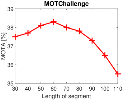
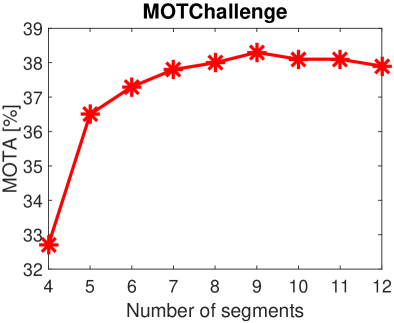
Figure 5: The effects of the segment’s parameters on MOTChallenge training set (Measured by MOTA score).

The effects of the segment’s parameters on the final performance are shown in Figure 5. For the number of segments, it is the average number of all the MOTChallenge training sequences. There is no overlap between segments. From the experiments, it is found that a segment of 50 to 80 frames works well for all the sequences.

IV-E Performance Evaluation

Evaluation: To show the effectiveness of joint learning and temporally constrained metrics, two baselines are designed. For Baseline 1, the Siamese CNN and the metrics are learned separately. We first learn the Siamese CNN alone by using the loss function (2), in which the $M$ is fixed as $M=I$. Then the common metric $M$ is learned separately with the features obtained from the previous learned Siamese CNN. No segment-wise metrics $M_{t}$ are learned for Baseline 1. For Baseline 2, the unified deep model without the temporally constrained multi-task mechanism is learned for tracklet affinity model. In Baseline 2, we use the loss function in Equation (2) instead of Equation (3) to learn the unified deep model. Moreover, to show the effectiveness of the CNN fine-tuning and the common metric $M_{0}$, two more baselines are designed. For Baseline 3, the Siamese CNN is pre-trained on JELMOLI dataset but without fine-tuning on target dataset using (3). The temporally constrained metrics and the Siamese CNN are learned separately. For Baseline 4, no common metric $M_{0}$ is used. The objective function (3) without the first term is used for this baseline. Note that the Siamese CNNs of all the baselines are pre-trained on JELMOLI dataset [33].

From Table III, IV, V and VI, it is found that Baseline 2 achieves overall better performance than Baseline 1 on the evaluated datasets, which proves the effectiveness of the joint learning. Moreover, our method achieves significant improvement in performance on the evaluated datasets, compared with Baseline 2, which validates the superiority of our unified deep model with the temporally constrained multi-task learning mechanism. Our method also achieves overall better performance than Baseline 3 and Baseline 4, which demonstrates the effectiveness of fine-tuning and adding the common metric $M_{0}$.

Method	MOTA	MOTP	Recall	Precision	FAF	FP	FN	GT	MT	PT	ML	Frag	IDS
Milan et al. [36]	90.6%	80.2%	92.4%	98.4%	0.07	59	302	23	91.3%	4.4%	4.3%	6	11
Berclaz et al. [37]	80.3%	72.0%	83.8%	96.3%	0.16	126	641	23	73.9%	17.4%	8.7%	22	13
Andriyenko et al. [38]	86.3%	78.7%	89.5%	97.6%	0.11	88	417	23	78.3%	17.4%	4.3%	21	38
Andriyenko et al. [39]	88.3%	79.6%	90.0%	98.7%	0.06	47	396	23	82.6%	17.4%	0.0%	14	18
Pirsiavash et al. [23]	77.4%	74.3%	81.2%	97.2%	0.12	93	742	23	60.9%	34.8%	4.3%	62	57
Wen et al. [7]	92.7%	72.9%	94.4%	98.4%	0.08	62	222	23	95.7%	0.0%	4.3%	10	5
Chari et al. [40]	85.5%	76.2%	92.4%	94.3%	-	262	354	19	94.7%	5.3%	0.0%	74	56
Baseline1	93.6%	86.3%	96.3%	97.7%	0.13	106	170	19	94.7%	5.3%	0.0%	18	18
Baseline2	94.3%	86.4%	96.6%	97.9%	0.12	94	157	19	94.7%	5.3%	0.0%	16	11
Baseline3	94.0%	86.3%	96.5%	97.8%	0.13	100	163	19	94.7%	5.3%	0.0%	20	12
Baseline4	94.7%	86.4%	97.1%	97.8%	0.13	103	134	19	94.7%	5.3%	0.0%	13	8
Ours	95.8%	86.4%	97.5%	98.4%	0.09	74	115	19	94.7%	5.3%	0.0%	8	4

TABLE III: Comparison of tracking results between state-of-the-art methods and ours on PETS 2009 dataset.

Method	MOTA	MOTP	Recall	Precision	FAF	FP	FN	GT	MT	PT	ML	Frag	IDS
Leal-Taixe et al. [41]	71.3%	71.8%	-	-	-	-	-	231	58.6%	34.4%	7.0%	363	165
Zhang et al. [22]	69.1%	72.0%	-	-	-	-	-	231	53.0%	37.7	9.3%	440	243
Benfold et al. [26]	64.3%	80.2%	-	-	-	-	-	231	67.4%	26.1%	6.5%	343	222
Pellegrini et al. [42]	65.5%	71.8%	-	-	-	-	-	231	59.1%	33.9%	7.0%	499	288
Wu et al. [43]	69.5%	68.7%	-	-	-	-	-	231	64.7%	27.4%	7.9%	453	209
Yamaguchi et al. [44]	66.6%	71.7%	-	-	-	-	-	231	58.1%	35.4%	6.5%	492	302
Possegger et al. [45]	70.7%	68.6%	-	-	-	-	-	231	56.3%	36.3%	7.4%	321	157
Baseline1	54.8%	72.5%	71.1%	85.0%	1.99	895	2068	231	58.0%	31.2%	10.8%	360	268
Baseline2	58.4%	73.0%	72.2%	87.5%	1.63	735	1983	231	59.7%	30.3%	10.0%	325	251
Baseline3	57.1%	72.8%	72.3%	86.5%	1.79	806	1979	231	58.9%	30.7%	10.4%	326	265
Baseline4	63.8%	74.0%	73.2%	90.8%	1.18	530	1915	231	62.8%	29%	8.2%	223	153
Ours	67.2%	74.5%	75.2%	92.6%	0.95	428	1770	231	65.8%	27.7%	6.5%	173	146

TABLE IV: Comparison of tracking results between state-of-the-art methods and ours on Town Centre dataset.

Method	MOTA	MOTP	Recall	Precision	FAF	FP	FN	GT	MT	PT	ML	Frag	IDS
Shu et al. [27]	74.1%	79.3%	81.7%	91.3%	-	-	-	14	-	-	-	-	-
Andriyenko et al. [38]	60.0%	70.7%	69.3%	91.3%	0.65	162	756	14	21.4%	71.5%	7.1%	97	68
Andriyenko et al. [39]	73.1%	76.5%	86.8%	89.4%	1.01	253	326	14	78.6%	21.4%	0.0%	70	83
Pirsiavash et al. [23]	65.7%	75.3%	69.4%	97.8%	0.16	39	754	14	7.1%	85.8%	7.1%	60	52
Wen et al. [7]	88.4%	81.9%	90.8%	98.3%	0.16	39	227	14	78.6%	21.4%	0.0%	23	21
Baseline1	76.5%	72.8%	86.0%	91.6%	0.78	195	344	14	71.4%	28.6%	0.0%	95	39
Baseline2	80.7%	72.6%	89.5%	92.3%	0.74	185	258	14	78.6%	21.4%	0.0%	63	33
Baseline3	79.7%	72.7%	89.1%	91.8%	0.78	196	269	14	78.6%	21.4%	0.0%	70	34
Baseline4	81.9%	72.7%	89.7%	93.1%	0.65	163	254	14	78.6%	21.4%	0.0%	59	30
Ours	85.7%	72.9%	92.4%	93.5%	0.63	158	188	14	78.6%	21.4%	0.0%	49	6

TABLE V: Comparison of tracking results between state-of-the-art methods and ours on ParkingLot dataset.

Method	MOTA	MOTP	Recall	Precision	FAF	FP	FN	GT	MT	PT	ML	Frag	IDS
Kuo et al. [4]	-	-	76.8%	86.6%	0.891	-	-	125	58.4%	33.6%	8.0%	23	11
Yang et al. [5]	-	-	79.0%	90.4%	0.637	-	-	125	68.0%	24.8%	7.2%	19	11
Milan et al. [46]	-	-	77.3%	87.2%	-	-	-	125	66.4%	25.4%	8.2%	69	57
Leal-Taixe et al. [47]	-	-	83.8%	79.7%	-	-	-	125	72.0%	23.3%	4.7%	85	71
Bae et al. [9]	72.03%	64.01%	-	-	-	-	-	126	73.8%	23.8%	2.4%	38	18
Baseline1	68.6%	76.8%	76.7%	90.7%	0.60	812	2406	125	56.8%	32.8%	10.4%	133	31
Baseline2	71.2%	77.0%	78.4%	91.8%	0.54	728	2236	125	60.8%	29.6%	9.6%	75	20
Baseline3	69.6%	76.9%	77.2%	91.3%	0.56	764	2358	125	58.4%	31.2%	10.4%	115	28
Baseline4	72.6%	77.2%	79.1%	92.6%	0.48	653	2161	125	62.4%	28.8%	8.8%	52	18
Ours	75.4%	77.5%	80.2%	94.5%	0.36	486	2050	125	68.8%	24.8%	6.4%	36	6

TABLE VI: Comparison of tracking results between state-of-the-art methods and ours on ETH dataset.

Method	MOTA	MOTP	FAF	FP	FN	GT	MT	PT	ML	Frag	IDS
DP_NMS [23]	14.5%	70.8%	2.3	13,171	34,814	721	6.0%	53.2%	40.8%	3090	4537
SMOT [6]	18.2%	71.2%	1.5	8,780	40,310	721	2.8%	42.4%	54.8%	2132	1148
CEM [36]	19.3%	70.7%	2.5	14,180	34,591	721	8.5%	45%	46.5%	1023	813
TC_ODAL [9]	15.1%	70.5%	2.2	12,970	38,538	721	3.2%	41%	55.8%	1716	637
ELP [48]	25.0%	71.2%	1.3	7,345	37,344	721	7.5%	48.7%	43.8%	1804	1396
CNNTCM (Ours)	29.6%	71.8%	1.3	7,786	34,733	721	11.2%	44.8%	44.0%	943	712

TABLE VII: Comparison of tracking results between state-of-the-art methods and ours on MOTChallenge Benchmark.

Method	MOTA	MOTP	Recall	Precision	FAF	FP	FN	GT	MT	PT	ML	Frag	IDS
DP_NMS [23]	29.7%	75.2%	31.4%	97.2%	0.09	1,742	130,338	1051	6.7%	37.4%	55.9%	1,738	1,359
SMOT [6]	33.8%	73.9%	43.5%	85.3%	0.72	14,248	107,310	1051	6.2%	58.1%	35.7%	5,507	4,214
CEM [36]	32.0%	74.2%	39.7%	85.1%	0.67	13,185	114,576	1051	11.1%	42.4%	46.5%	2,016	1,367
TC_ODAL [9]	32.8%	73.2%	56.2%	71.3%	2.17	42,913	83,206	1051	21.9%	48.1%	30.0%	3,655	1,577
ELP [48]	34.1%	75.9%	40.2%	89.2%	0.47	9,237	113,590	1051	9.4%	43.9%	46.7%	2,451	2,301
CNNTCM (Ours)	39.0%	74.5%	41.7%	95.1%	0.20	4,058	110,635	1051	11.9%	43.2%	44.9%	1,946	1,236

TABLE VIII: Comparison of tracking results between state-of-the-art methods and ours on the new dataset.

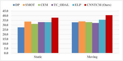
(a) Camera motion

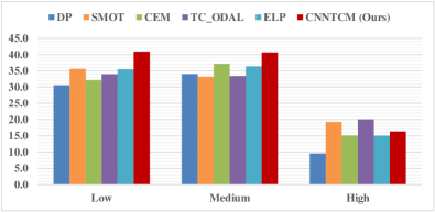
(b) Viewpoint

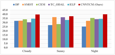
(c) Weather conditions

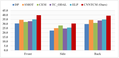
(d) Pedestrian view

Figure 6: Comparison of the evaluated tracking methods under different conditions in terms of MOTA score (%).

We further evaluate our method on the recent MOTChallenge 2D Benchmark [29]. The qualitative results of our method (CNNTCM) are available on the MOTChallenge Benchmark website [49]. From Table VII, it is found that our method achieves better performance on all evaluation measures compared with a recent work [6] which is also based on the GLA framework. Compared with other state-of-the-art methods, our method achieves better or comparable performance on all the evaluation measures.

Moreover, to further show the generality and effectiveness of the proposed method on large-scale sequences, a new dataset with 40 diverse sequences is built for performance evaluation. 5 state-of-the-art tracking methods with released source codes are used in evaluation for the new dataset. The parameters of each evaluated tracking method are fine-tuned on the 10 training sequences. As shown in Table VIII, our method achieves the best performance on MOTA and IDS, which are the most two direct measures for tracklet association evaluation, among all the evaluated tracking methods. The comparison of tracking results between these five state-of-the-art methods and ours on the new dataset under different conditions is shown in Figure 6.

Computational speed: Our system was implemented using the MatConvNet toolbox [50] on a server with a 2.60GHz CPU and a Tesla K20c GPU. The computation speed is subject to the number of targets in a video sequence. The speeds of our method are about 0.38, 0.81, 0.50, 0.60, 0.59, 0.55 (sec/frame) for PETS 2009, Town Centre, ParkingLot, ETH, MOTChallenge, and the new dataset, respectively, excluding the detection step. Note that speed-up can be achieved by further optimization of the codes.

V Conclusion

In this paper, a novel unified deep model for tracklet association is presented. This deep model can jointly learn the Siamese CNN and temporally constrained metrics for tracklet affinity models. The experimental results of Baseline 1 and Baseline 2 validate the effectiveness of the joint learning and the temporally constrained multi-task learning mechanism of the proposed unified deep model. Baseline 3 and Baseline 4 demonstrate the effectiveness of fine-tuning and adding the common metric. Moreover, a new large-scale dataset with 40 fully annotated sequences is created to facilitate multi-target tracking evaluation. Furthermore, extensive experimental results on five public datasets and the new large-scale dataset compared with state-of-the-art methods also demonstrate the superiority of our method.

References

- [1] N. Dalal and B. Triggs, “Histograms of oriented gradients for human detection,” in CVPR, 2005.
- [2] X. Wang, T. X. Han, and S. Yan, “An hog-lbp human detector with partial occlusion handling,” in ICCV, 2009.
- [3] P. Felzenszwalb, R. Girshick, D. McAllester, and D. Ramanan, “Object detection with discriminatively trained part based models,” IEEE Transactions on Pattern Analysis and Machine Intelligence, vol. 32, no. 9, pp. 1627–1645, 2010.
- [4] C. H. Kuo and R. Nevatia, “How does person identity recognition help multi-person tracking?” in CVPR, 2011.
- [5] B. Yang and R. Nevatia, “An online learned crf model for multi-target tracking,” in CVPR, 2012.
- [6] C. Dicle, O. Camps, and M. Sznaier, “The way they move: tracking multiple targets with similar appearance,” in ICCV, 2013.
- [7] L. Wen, W. Li, J. Yan, Z. Lei, D. Yi, and S. Z. Li, “Multiple target tracking based on undirected hierarchical relation hypergraph,” in CVPR, 2014.
- [8] B. Wang, G. Wang, K. L. Chan, and L. Wang, “Tracklet association with online target-specific metric learning,” in CVPR, 2014.
- [9] S. H. Bae and K. J. Yoon, “Robust online multi-object tracking based on tracklet confidence and online discriminative appearance learning,” in CVPR, 2014.
- [10] A. Krizhevsky, I. Sutskever, and G. Hinton, “Imagenet classification with deep convolutional neural networks,” in NIPS, 2012.
- [11] R. Girshick, J. Donahue, T. Darrell, and J. Malik, “Rich feature hierarchies for accurate object detection and semantic segmentation,” in CVPR, 2014.
- [12] D. Shmoys and E. Tardos, “An approximation algorithm for the generalized assignment problem,” Mathematical Programming, vol. 62, no. 1, pp. 461–474, 1993.
- [13] S. Gold and A. Rangarajan, “Softmax to softassign: Neural network algorithms for combinatorial optimization,” Journal of Artificial Neural Nets, vol. 2, no. 4, pp. 381–399, 1995.
- [14] M. Oquab, L. Bottou, I. Laptev, and J. Sivic, “Learning and transferring mid-level image representations using convolutional neural networks,” in CVPR, 2014.
- [15] N. Wang and D. Y. Yeung, “Learning a deep compact image representation for visual tracking,” in NIPS, 2013.
- [16] H. Li, Y. Li, and F. Porikli, “Deeptrack: Learning discriminative feature representations by convolutional neural networks for visual tracking,” in BMVC, 2014.
- [17] L. Wang, T. Liu, G. Wang, K. L. Chan, and Q. Yang, “Video tracking using learned hierarchical features,” IEEE Transactions on Image Processing, vol. 24, no. 4, pp. 1424–1435, 2015.
- [18] K. Zhang, Q. Liu, Y. Wu, and M. H. Yang, “Robust tracking via convolutional networks without learning,” arXiv preprint, vol. arXiv:1501.04505, 2015.
- [19] S. Hong, T. You, S. Kwak, and B. Han, “Online tracking by learning discriminative saliency map with convolutional neural network,” arXiv preprint, vol. arXiv:1502.06796, 2015.
- [20] C. Huang, B. Wu, and R. Nevatia, “Robust object tracking by hierarchical association of detection responses,” in ECCV, 2008.
- [21] Y. LeCun, L. Bottou, Y. Bengio, and P. Haffner, “Gradient-based learning applied to document recognition,” Proc. of the IEEE, 1998.
- [22] L. Zhang, Y. Li, and R. Nevatia, “Global data association for multi-object tracking using network flows,” in CVPR, 2008.
- [23] H. Pirsiavash, D. Ramanan, and C. Fowlkes, “Globally-optimal greedy algorithms for tracking a variable number of objects,” in CVPR, 2011.
- [24] A. Butt and R. T. Collins, “Multi-target tracking by lagrangian relaxation to min-cost network flow,” in CVPR, 2013.
- [25] J. Ferryman and A. Shahrokni, “Pets2009: Dataset and challenge,” in Winter-PETS, 2009.
- [26] B. Benfold and I. Reid, “Stable multi-target tracking in real-time surveillance video,” in CVPR, 2011.
- [27] G. Shu, A. Dehghan, O. Oreifej, E. Hand, and M. Shah, “Part-based multiple-person tracking with partial occlusion handling,” in CVPR, 2012.
- [28] A. Ess, K. S. B. Leibe, and L. van Gool, “Robust multiperson tracking from a mobile platform,” IEEE Transactions on Pattern Analysis and Machine Intelligence, vol. 31, no. 10, pp. 1831–1846, 2009.
- [29] L. Leal-Taixe, A. Milan, I. Reid, S. Roth, and K. Schindler, “Motchallenge 2015: Towards a benchmark for multi-target tracking,” arXiv preprint, vol. arXiv: 1504.01942, 2015.
- [30] M. Andriluka, S. Roth, and B. Schiele, “People-tracking-by-detection and people-detection-by-tracking,” in CVPR, 2008.
- [31] A. Geiger, P. Lenz, and R. Urtasun, “Are we ready for autonomous driving? the kitti vision benchmark suite,” in CVPR, 2012.
- [32] Y. Wu, J. Lim, and M. H. Yang, “Online object tracking: a benchmark,” in CVPR, 2013.
- [33] A. Ess, B. Leibe, and L. van Gool, “Depth and appearance for mobile scene analysis,” in ICCV, 2007.
- [34] Y. Li, C. Huang, and R. Nevatia, “Learning to associate: Hybridboosted multi-target tracker for crowded scene,” in CVPR, 2009.
- [35] K. Bernardin and R. Stiefelhagen, “Evaluating multiple object tracking performance: The clear mot metrics,” EURASIP J. Image and Video Processing, 2008.
- [36] A. Milan, S. Roth, and K. Schindler, “Continuous energy minimization for multi-target tracking,” IEEE Transactions on Pattern Analysis and Machine Intelligence, vol. 36, no. 1, pp. 58–72, 2014.
- [37] J. Berclaz, F. Fleuret, E. Turetken, and P. Fua, “Multiple object tracking using k-shortest paths optimization,” IEEE Transactions on Pattern Analysis and Machine Intelligence, vol. 33, no. 9, pp. 1806–1819, 2011.
- [38] A. Andriyenko and K. Schindler, “Multi-target tracking by continuous energy minimization,” in CVPR, 2011.
- [39] A. Andriyenko, K. Schindler, and S. Roth, “Discrete-continuous optimization for multi-target tracking,” in CVPR, 2012.
- [40] V. Chari, S. L. Julien, I. Laptev, and J. Sivic, “On pairwise costs for network flow multi-object tracking,” in CVPR, 2015.
- [41] L. Leal-Taixe, G. Pons-Moll, and B. Rosenhahn, “Everybody needs somebody: Modeling social and grouping behavior on a linear programming multiple people tracker,” in ICCV Workshops, 2011.
- [42] S. Pellegrini, A. Ess, K. Schindler, and L. V. Gool, “You’ll never walk alone: modeling social behavior for multi-target tracking,” in ICCV, 2009.
- [43] Z. Wu, J. Zhang, and M. Betke, “Online motion agreement tracking,” in BMVC, 2013.
- [44] K. Yamaguchi, A. C. Berg, L. E. Ortiz, and T. L. Berg, “Who are you with and where are you going?” in CVPR, 2011.
- [45] H. Possegger, T. Mauthner, P. M. Roth, and H. Bischof, “Occlusion geodesics for online multi-object tracking,” in CVPR, 2014.
- [46] A. Milan, K. Schindler, and S. Roth, “Detection- and trajectory-level exclusion in multiple object tracking,” in CVPR, 2013.
- [47] L. Leal-Taixe, M. Fenzi, A. Kuznetsova, B. Rosenhahn, and S. Savarese, “Learning an image-based motion context for multiple people tracking,” in CVPR, 2014.
- [48] N. McLaughlin, J. M. D. Rincon, and P. Miller, “Enhancing linear programming with motion modeling for multi-target tracking,” in WACV, 2015.
- [49] “Multiple object tracking benchmark,” http://motchallenge.net/.
- [50] A. Vedaldi and K. Lenc, “Matconvnet – convolutional neural networks for matlab,” arXiv preprint, vol. arXiv:1412.4564, 2014.