The Accretion Flow - Discrete Ejection Connection in GRS 1915+105

Abstract

The microquasar GRS 1915+105 is known for its spectacular discrete ejections. They occur unexpectedly, thus their inception escapes direct observation. It has been shown that the X-ray flux increases in the hours leading up to a major ejection. In this article, we consider the serendipitous interferometric monitoring of a modest version of a discrete ejection described in Reid et al. (2014) that would have otherwise escaped detection in daily radio light curves. The observation begins $\sim 1$ hour after the onset of the ejection, providing unprecedented accuracy on the estimate of the ejection time. The astrometric measurements allow us to determine the time of ejection as $\rm{MJD}\,56436.274^{+0.016}_{-0.013}$, i.e., within a precision of 41 minutes (95% confidence). Just like larger flares, we find that the X-ray luminosity increases in last 2 - 4 hours preceding ejection. Our finite temporal resolution indicates that this elevated X-ray flux persists within $21.8^{+22.6}_{-19.1}$ minutes of the ejection with 95% confidence, the highest temporal precision of the X-ray - superluminal ejection connection to date. This observation provides direct evidence that the physics that launches major flares occurs on smaller scales as well (lower radio flux and shorter ejection episodes). The observation of a X-ray spike prior to a discrete ejection, although of very modest amplitude suggests that the process linking accretion behavior to ejection is general from the smallest scales to high luminosity major superluminal flares.

1 Introduction

One of the most striking features of Galactic black holes (GBHs) are the major radio flares. These are large increases in radio flux that appear to be rapidly moving discrete components in followup radio interferometric observations (Mirabel and Rodriguez, 1994; Fender et al., 1999; Dhawan et al., 2000; Miller-Jones et al., 2005, 2012). Major flare ejections (MFEs) of rapidly moving components are rare states that occur as brief transients in some GBHs. The physics of the launching mechanism that produces these dramatic events has been the subject of much speculation (Fender et al., 2004; Punsly and Rodriguez, 2013b). The primary hurdle to understanding the physics of these powerful events is that they occur unexpectedly and are quite brief in their inception. Thus, X-ray telescopes and radio interferometers are never both pointing at these objects at the precise instance of ejection. Consequently, the connection between the accretion state (the X-ray emission) and discrete superluminal ejections has been hampered by the coarse daily monitoring of these events that evolve on time scales on the order of hours or minutes. As such, there is not an agreed upon understanding of the state of the accretion disk at the time of ejection.

In terms of producing MFEs, GRS 1915+105 is far and away the most prolific. Consequently, there is a wealth of observational information from monitoring and pointed observations. Increases in the X-ray light curve have been associated with MFEs based on daily monitoring (Namiki et al, 2006). Yet, the coarse time resolution makes it unclear if the X-ray increases occurred during, after or following the ejection episode. This is a critical distinction for theorists who are trying to understand the physical mechanism of the MFEs. The situation is further clouded by efforts to unify jet phenomena. There is high time resolution (minutes and seconds) monitoring of oscillatory events that are discussed in an inclusive context with MFEs, eg. (Fender and Belloni, 2004). The notion of X-ray dips preceding superluminal ejections has become a well accepted notion. Yet, in the study of these oscillatory events, they are so brief and weak that no apparent motion has ever been directly detected with a radio interferometer. The notion is so popular that in the highly publicized work of Marscher et al. (2002) they claimed that they detected X-ray dips preceding superluminal ejections in the active galactic nucleus of the Seyfert galaxy 3C120 and this was direct evidence of a commonality with GRS 1915+105. This is one of the most cited pieces of evidence supporting the notion of scale invariance in black hole physics from stellar massive black holes to supermassive black holes. Our detailed study of an ejection in GRS 1915+105 aims improve our understanding of the putative accretion disk - superluminal ejection connection.

In a quest to understand the physics of the discrete ejections, we have been studying the X-ray time evolution immediately preceding flare production and during the ejections in GRS 1915+105 (Punsly and Rodriguez, 2013a, c; Punsly Rodriguez and Trushkin, 2014). The data being all serendipitous is not ideal, but we have reached and reaffirmed certain conclusions:

1. A conspicuous peak in X-ray flux occurs in the hours preceding the launch of the MFE.

2. During the ejection, the X-ray flux is highly variable.

3. Typically, there is a dip in the X-ray flux during the ejection, well below the pre-launch flux.

4. The time averaged X-ray flux during the ejection is correlated with the flux preceding the ejection with a similar, but slightly smaller, magnitude.

5. The X-ray light curve during the MFE often has large local maxima which can exceed the X-ray flux before the launch. These maxima can occur either during the ejection or immediately after the ejection episode.

The examination of these findings in the past has been hampered by crude temporal sampling. MFE ejection times have been estimated from radio light curves. There is an inherent ambiguity in that optically thick ejections will not show an increase in the light curve until they expand to become optically thin at the observing frequency. Thus, they are not precise. Historically, triggered radio interferometry initiates $>24$ hrs. after an ejection. Thus, extrapolating the trajectory of the moving plasmoids back in time for $>1$ day leads to large uncertainties in the ejection time. Furthermore, only the strongest MFEs ($>175$ mJy at 2.3 GHz) have been studied in the past since one needs a definite strong signal above the random radio fluctuations of the active source in GRS 1915+105 in order to determine if one has a certain detection of a MFE (Dhawan et al, 2004).

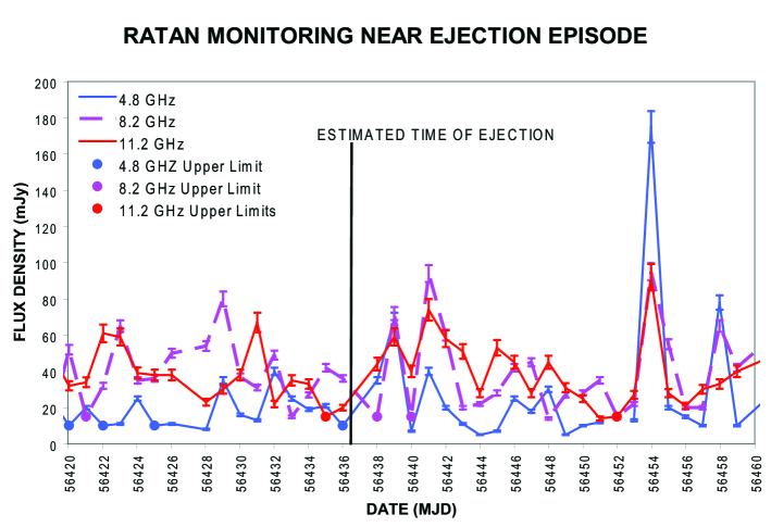
Figure 1: The RATAN-600 light curve around the time of the discrete ejection.

We present much more accurate temporal data than has previously been available of a MFE. We also are able to extend some of the trends that were noted above to a much weaker ejection. We fortunately have multi-epoch, snapshot, Very Long Baseline Array (VLBA) observations of a slightly superluminal ejection with the data sampling beginning $\sim$1 hour after the onset of the ejection, that were already published in Reid et al. (2014). We re-analyze here these data following a slightly different procedure. We adopt the original strategy to place this VLBA observation in a context of radio monitoring with the RATAN telescope and confront this radio flare to contemporaneous X-ray observations obtained from the MAXI all sky monitor (http://maxi.riken.jp/mxondem/). The MAXI observatory typically observes GRS 1915+105 every 1.5 hours and it can potentially provide useful spectral data in the energy range 1 keV - 20 keV (Matsuoka et al., 2009). We have downloaded the MAXI data that occurred within minutes of the ejection as well as two hours before and one hour after the ejection began. The results of our data analysis are found in Section 4.

2 Radio Monitoring

GRS 1915+105 was observed with the RATAN-600 radio telescope at 4.8, 8.2 and 11.2 GHz as part of our 2013 monitoring campaign. The details of these observations have been described elsewhere (Trushkin et al., 2008; Punsly Rodriguez and Trushkin, 2014). The secondary calibrators 3C286 and PKS1345+12 were used for daily calibration. The temporal spacing of our monitoring program – one measurement per day – is far too large to estimate the time of the major ejection that is associated with the radio flare. From Punsly and Rodriguez (2013a) and Figure 1, determination of the ejection initiation and end times require temporal resolution 100 times finer, on the order of an hour or minutes. However, strong flares are luminous for at least 1 day, so it is adequate for identifying major ejections (Rodriguez and Mirabel, 1999; Miller-Jones et al., 2005). Figure 1 shows the light curve near the “suggested” time of the ejection detected with VLBA on MJD 56436.3 (Reid et al., 2014). The radio flux density is low as expected a few hours before the ejection. The increase in the low frequency flux at 4.8 GHz, 1.7 days after the ejction, is consistent with the later stages of a discrete ejection. However, the flux levels are so low for this event and the time sampling so coarse that the identification cannot be made with certainty.

3 The VLBA Observations

GRS 1915+105 was observed with VLBA at 22.2 GHz on May 24, 2013 (MJD 56436). The data from the 8 continental VLBA stations were imaged in 7 individual 20 minute scans. In order to track the motion of the ejection, “snapshots” were made from the VLBA observation which have $\sim 20$ interferometer (u,v)-points. With the sparse u-v coverage only peak fluxes were detectable. One component was detected and its trajectory is plotted from the data in Reid et al. (2014) in Figure 2. The peak flux density at 22.2 GHz was $~{}6.7\pm 0.8$ mJy for 6 of the 7 snapshots. The third (outlier) data point with the larger error bars was $\lesssim 2$ mJy. The core was not detected and a conservative upper limit of 3 mJy is placed on its flux density.

The trajectory provides information on the the point of origin for the ejection. There are three things to consider in establishing the location of the point of origin.

1. Accuracy of Origin Based on Proper Motion: The expected 22.2 GHz core position based on the parallax and proper motion fitting results of Reid et al. (2014) yield the origin of the plot (which is not necessarily the point of origin of the ejection). The uncertainty associated with its location is ($\Delta$RA, $\Delta$Dec) = (0.055 mas, 0.100 mas).

2. Optical Depth Effects: The radio core detected in the parallax measurements is detected at high frequency (22.2 GHz) and the data has been checked for a constant flux over the observations in order to validate the application of a Fourier transformation of the interferometer data (Reid et al., 2014). The indication is that the detections are most likely the optically thick emission commonly associated with a compact jet (Klein-Wolt et al, 2002; Rushton et al., 2010b; Gallo et al., 2003). Thus, one does not see the point of origin, but the synchrotron self absorption (SSA) optical depth, $\tau\sim 1$ surface. Modeling the source of multiple compact jets in GRS 1915+105 in Punsly and Rodriguez (2016) consistently indicated that the peak of the 15 GHz flux density was $\approx 0.3$ mas from the true position of jet origin. Likewise, we expect that the peak of the 22.2 GHz emission is offset from the true point of origin for the putative compact jets detected by parallax observations. However, being much weaker than the compact jets considered in the previous models of Punsly and Rodriguez (2016), the dimensions are likely smaller. Previous jets were $\sim 10$ times brighter than the putative compact jets monitored for the parallax measurements (Reid et al., 2014). The surface area of the $\tau\sim 1$ surface scales with the luminosity (in a highly modeled dependent manner). Thus, we expect the magnitude of the core shift to be smaller as well. Furthermore, there is less opacity at higher frequency and highly simplified models of jets indicate that the core shifts scales like the observing frequency as $\nu^{-1}$ (Blandford and Köingl, 1979). There are two effects, a smaller dimension in the weaker compact jets and an upstream shift of the core towards its true position due to less optical depth at 22.2 GHz. We incorporate this broad range of possible upstream dislocations by placing the point of jet origin, corrected for optical depth effects, to be at $\approx 0.2\pm 0.1$ mas upstream of the proper motion estimated 22 GHz peak flux density position.

3. Statistical Scatter in the Fit to the Trajectory. The trajectory is estimated from a least squares fit with uncertainty in both variables. The data scatter leads to an uncertainty in the best fit trajectory.

Our first step in the determination of the ejection time is to fit the data by a linear least squares with uncertainty in both variables (Reed, 1989). Unlike Reid et al. (2014), we do not exclude the outlier point. The best fit to the data scatter in Figure 2 is the solid line and the dashed lines show the 95% confidence contours of the fit. The next step is to find the radio core adjusted for optical depth effects based on points 1 and 2 above. We displace the origin 0.2 mas upstream of the point (0, 0) parallel to the direction given by the slope of the trajectory obtained from our least squares fit. We find the shifted radio core location based on astrometry and the shift due to optical depth to be at ($0.15\pm 0.09$ mas, $0.13\pm 0.12$ mas), where the errors are obtained by adding the errors in points 1 and 2 above in quadrature. This shifted astrometric core location is noted by the red cross in the upper right hand corner of Figure 2. The cross represents the 95% confidence for the spatial location (i.e., 2$\sigma$) of the shifted astrometric core. We have two 95% confidence contours, one for the astrometric core shifted by $0.2\pm 0.1$ mas and one for the trajectory of the ejection. The intersection of these two 95% confidence contours provides our 95% confidence contour for the point of origin for the ejection shown as the blue triangle. Using the centroid as the best choice for the point of origin, we find that it is located at ($0.22^{+0.11}_{-0.22}$ mas, $0.02^{+0.11}_{-0.13}$ mas) with 95% confidence.

Using this estimate for the point of origin for the jet, we can compute the time of the ejection by plotting the displacement from the point of origin versus time and extrapolating backwards in time. This is done in Figure 3. The least squares fit with uncertainty in both variables is given by the solid line with the 95% contours shown as the dashed lines. The slope of the line is 0.97 mas/hr. The time of origin from the fit is MJD $56436.274\pm 0.012$. However, this does not include the uncertainty that is associated with the point of origin noted at the end of the paragraph above. Using the speed of the ejection from the slope of the best linear fit to the observed relationship in Figure 3, we can translate the uncertainty in location of the point of origin to an uncertainty in time and add this uncertainty in quadrature with the uncertainty associated with the fit. We obtain a 95% confidence contour for the time of ejection,

$$\rm{EJECTION\;TIME}=\rm{MJD}\,56436.274^{+0.016}_{-0.013}\;.$$ (1)

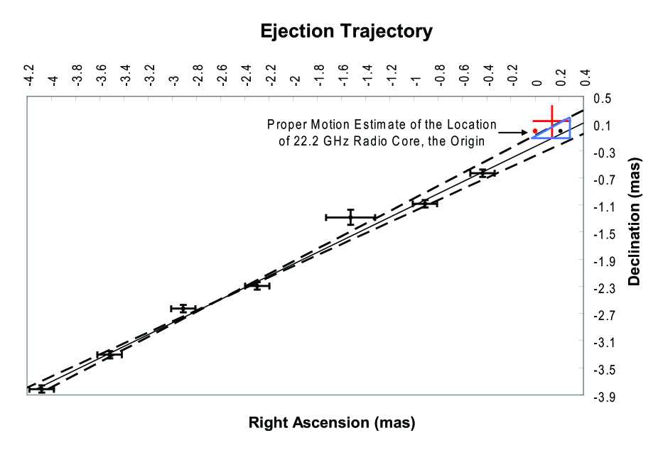
Figure 2: The trajectory of the ejection from a series 22.2 GHz VLBA snapshot images on MJD 56436. The 22.2 GHz radio core (the red dot) was not detected, but its position is estimated from a series of proper motion measurements used in the parallax observations of GRS 1915+105 (Reid et al., 2014). Optical depth effects shift the true core position upstream (parallel to the jet trajectory) by an amount that we estimate from an analysis of 15 GHz VLBA images to be $0.2\pm 0.1$ mas. The red cross represents the 95% confidence contour for this location. The dashed lines are the 95% confidence contours for the least squares fit with uncertainty in both variables of the VLBA determined trajectories. The intersection of the two independent sets of 95% confidence contours provides our 95% confidence contour for the the point of origin for the ejection that is bounded by the blue triangle. The black dot, the centroid of the triangle, is our best estimate of the position of the point of origin of the discrete ejection.

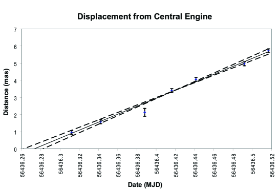
Figure 3: The displacement of the discrete ejection from the point of origin estimated in Figure 2. The data is fit by least squares with uncertainty in both variables. The uncertainty in the time measurement (10 minutes) is less than the size of the data point and uniform.

Because the precise timing of the X-ray variations and the ejection time is critical in order to extract the physical mechanism responsible for discrete ejections, the exercise above is necessary. The method used by Reid et al. (2014), while providing results consistent with ours, suffers from a high uncertainty on the true core position leading to slightly different times of ejection when considering the North-South and East-West ejections. Here by precisely re-setting the origin of the ejection we strengthen and refine the zero-time of the ejection. Figure 2 shows that our estimated point of origin for the jet is $\approx 1\sigma$ from the estimated radio core position. This type of accuracy is essential for understanding the precise timing of the event.

4 MAXI Observations

We downloaded the data from the MAXI pipeline around the time of the ejection. The light curves of the 2.0 keV - 6.0 keV count rates and the 2.0 keV -20 keV count rates are plotted in Figure 4. The ejection time estimated in the last section is indicated by the dotted black vertical line. The thickness represents the range of uncertainty. For more than 24 hours GRS 1915+105 is in a low X-ray state from MJD 56435.047 to MJD 56436.080. Typically, data is taken every 1.5 hours, but a key data point was missed after this. Thus, with this limitation, we note that 4 hours later the X-ray flux is at a maximum. The X-ray luminosity peak occurs on MJD 56436.259. Comparing this date to Equation (1), this elevated X-ray flux precedes the onset of the ejection by $21.8^{+22.6}_{-19.1}$ minutes with 95% confidence. This is the finest and most accurately determined juxtaposition in time of an X-ray spike and a MFE. We have clearly verified point 1 from the Introduction. The flux and count rate in both the 2.0 keV - 6.0 keV and 2.0 keV - 20.0 keV windows increases by $\gtrsim 100\%$ in $<4.3$ hrs (Table 1 and Figure 3). It is uncertain if the ejection is still taking place during the next MAXI observation on MJD 56436.323.

Based on our estimate of the ejection time above, we use the MAXI spectral data to look for spectral evolution before and during ejection. The sensitivity of MAXI is low (low effective area), and we needed to bin the data over the quiescent period preceding the flare in order to better constrain the spectral fits. This was acceptable because the source was slowly varying in time. Our spectral fits are based on an absorbed powerlaw model (tbabs*powerlaw in XSPEC terminology) with abundances obtained from Wilms et al. (2000). The absorbed powerlaw model applied to the MAXI data from 1 keV to 20 keV are described in Table 1. The first column gives the date of the observation. The next column is the fitted column density of hydrogen, $N_{H}$. The third column is the photon index of the power law fit to the data, $\Gamma$. Columns four and five are the absorbed flux and the unabsorbed (intrinsic) flux that results from removing the absorbing effects of $N_{H}$, respectively. The last column is the reduced $\chi^{2}$ of the fit. The errors on the fitted parameters are at 90% confidence.

Table 1: Parametric Fits to MAXI Data Near the Flare Ejection

Date	$N_{H}$	$\Gamma$	Observed Flux	Intrinsic Flux	Reduced
			1 - 10 keV	1 - 10 keV	$\chi^{2}$(dof)
MJD	$10^{22}\mathrm{cm}^{-2}$		$10^{-8}\mathrm{ergs}/\mathrm{sec-}\mathrm{cm}^{2}$	$10^{-8}\mathrm{ergs}/\mathrm{sec-}\mathrm{cm}^{2}$
$56436.05\pm 0.04$	$7.2^{+2.3}_{-1.9}$	$2.4\pm 0.2$	$1.0$	$2.7$	0.69(26)
$56436.18\pm 0.02$	$8.8^{+2.8}_{-2.2}$	$2.8\pm 0.3$	$1.5$	$5.4$	0.89(20)
$56436.26\pm 0.01$	$8.1^{+2.3}_{-1.8}$	$2.7\pm 0.2$	$2.0$	$6.4$	1.15(25)
$56436.65\pm 0.01$	$6.2^{+3.5}_{-2.9}$	$2.4\pm 0.3$	$1.5$	$3.7$	0.3(20)

There are some evident trends in Table 1 for the 56436.27 flare. Obviously, the luminosity increases before the ejection. But, we also see $\Gamma$ steepens preceding the flare. This was observed in MFEs previously observed with MAXI (Punsly Rodriguez and Trushkin, 2014). The uncertainty in the photon index in Table 1 makes this phenomenon less than statistically significant. We do not see an increase in $N_{H}$ immediately before the flare as previously observed with MAXI (Punsly Rodriguez and Trushkin, 2014). The combination of a weak flare and the low sensitivity of MAXI makes the spectral analysis difficult and it might be that for such a weak flare that trends are undetectable with any significance. We also note a few limitations of the data. First, the fit to the last data entry in Table 1 is poor. There are just not enough counts to get good spectral information. Binning or combining observations is unfortunately not possible here, there is only the one widely spaced observation (shown in Figure 4) over the next two days. Furthermore, the changes are so rapid and the fluxes so low for this flare that it has poor statistics.

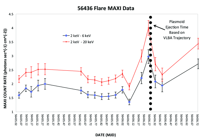
Figure 4: The MAXI light curve near the time of the flare. Note the X-ray flux peak near the time of the ejection.

5 Discussion

In this article, we re-examined a VLBA observation beginning $\sim 1$ hr after the onset of the ejection of a plasmoid of modest luminosity in order to explore the disk-jet connection for superluminal ejections with unprecedented accuracy. We used this fortunate circumstance in combination with X-ray monitoring with MAXI to verify that an increase in X-ray luminosity preceded the ejection. We were able to verify that the X-ray flux begins to increase 2 - 4 hours before the ejection and the elevated flux persists within $21.8^{+22.6}_{-19.1}$ minutes of the onset of the ejection with 95% confidence. This is one of the five X-ray properties (listed in the Introduction) detected before in larger MFEs with coarse time resolution of X-ray coverage and much coarser estimates of the times of ejection. The other four properties noted in the Introduction could not be verified, due to the fact that the ejection was relatively weak and brief and the MAXI time resolution and sensitivity were not adequate. The most interesting aspect eluded us due to insufficient time sampling of the X-ray data: when does the rise in X-ray luminosity end relative to the ejection time? We performed time resolved spectroscopy with MAXI even though the count rates were generally small to moderate. We did see a trend (although not statistically significant with the low number of counts) previously detected with MAXI that the spectral index of the X-ray power-law steepens when the X-ray luminosity increases before ejection (Punsly Rodriguez and Trushkin, 2014).

Our results suggest a possible link between weak radio “bubbles” and MFEs. Firstly, weak radio “bubbles” with flux densities of 10 mJy - 60 mJy at 15 GHz have been associated with X-ray cycles in X-ray classes $\nu$, $\lambda$, $\kappa$ and $\beta$ (Rodriguez et al, 2008a, b). X-ray spikes occur on the order of seconds to minutes before an increase in radio flux occurs. The spikes are accompanied by a softening of the X-ray spectrum similar to the spectral steepening seen here and in other MAXI observations of MFEs (Punsly Rodriguez and Trushkin, 2014). The discrete ejection observed here is $\approx 45$ mJy at 8.2 GHz (1.7 days after the ejection according to Figure 1) and forms a possible example of a common ejection mechanism that straddles the luminosity gap between the fainter “bubbles” ejections and the brighter MFEs. Furthermore, the phenomena of an X-ray spike preceding ejections seems to extend to stronger radio emission, up to 120 mJy in other quasi-periodic cycles (Prat et al, 2010). However, we note that no discrete ejections were monitored. The unification of these phenomenon has some significant discrepancies. The single discrete ejection discussed here and MFEs are temporally different from quasi-periodic episodes described in (Rodriguez et al, 2008a, b; Prat et al, 2010; Dhawan et al., 2000). There is no cycle, the event happened once. Also, the time scale for the X-ray spike to grow is much larger for the one time discrete ejections than for quasi-periodic cycles (Prat et al, 2010). Furthermore, strong quasi-periodic radio states showed no discrete components in VLBA monitoring (Dhawan et al., 2000). The radio image is morphologically similar to a blow-torch flame with no concentrations of intensity. This might be an artifact of blurring from multiple ejections moving a beam width in $\sim 1$ hour and poor u-v coverage from only 10 antennas.

References

- Blandford and Köingl (1979) Blandford, R. and Königl, A. 1979, ApJ 232 34
- Dhawan et al. (2000) Dhawan, V., Mirabel, I.F., Rodriguez, L. 2000, ApJ 343 373
- Dhawan et al (2004) Dwahan, V., Muno, M., Remillard, R. 2004, in X-Ray Timining 2003 Rossie and Beyond AIP Conference Proceedings, Volume 714, pp.150-153 (2004)
- Fender et al. (1999) Fender, R. et al., 1999, MNRAS 304 865
- Fender et al. (2004) Fender, R., Belloni, T., Gallo, E. 2004, MNRAS 355 1105
- Fender and Belloni (2004) Fender, R., Belloni, T. 2004, ARA&A, 42, 317
- Gallo et al. (2003) Gallo, E., Fender, R., Pooley, G. 2003, MNRAS 344 60
- Klein-Wolt et al (2002) Klein-Wolt et al., 2002, MNRAS 331 745
- Marscher et al. (2002) Marscher, A., Jorstad, S., G omez, J.-L., Aller, M. F., Ter asranta, H., Lister, M., Stirling, A., 2002, Nature 417, 625
- Matsuoka et al. (2009) Matsuoka, M. et al.., 2009, PASJ, 61, 999
- Miller-Jones et al. (2005) Miller-Jones, J. et al. 2005, MNRAS 363 867
- Miller-Jones et al. (2012) Miller-Jones, J. et al. 2012, MNRAS 421 468
- Mirabel and Rodriguez (1994) Mirabel, I.F., Rodriguez, L. 1994, Nature 371 46
- Namiki et al (2006) Namiki, M., Trushkin, S., Kotani, T., Kawai, N., Bursov, N., Fabrika, S. 206, VI Microquasars Workshop: Microquasars and Beyond, September 18-22, 2006, Societa del Casino, Como, Italy PoS(MQW96)083
- Prat et al (2010) Prat, L., Rodriguez, J, and Pooley, G. 2010, ApJ 717 1222
- Punsly and Rodriguez (2013a) Punsly, B., Rodriguez J. 2013a, ApJ 764 173
- Punsly and Rodriguez (2013b) Punsly, B., Rodriguez J. 2013b, ApJ 770 99
- Punsly and Rodriguez (2013c) Punsly, B., Rodriguez J. 2013c, MNRAS 435 2322
- Punsly and Rodriguez (2016) Punsly, B., Rodriguez J. 2016, to appear in ApJ http://arxiv.org/abs/1603.07675
- Punsly Rodriguez and Trushkin (2014) Punsly, B., Rodriguez J., Trushkin¡ S. 2014, ApJ 783 133
- Reed (1989) Reed, B. 1989, Am. J. Phys. 57 642
- Reid et al. (2014) Reid, M. et al. 2014, ApJ 796 2
- Rodriguez and Mirabel (1999) Rodriguez, L., Mirabel, I.F. 1999, ApJ 511 398
- Rodriguez et al (2008a) Rodriguez, J. et al 2008, ApJ 675 1436
- Rodriguez et al (2008b) Rodriguez, J. et al 2008, ApJ 675 1449
- Rushton et al. (2010a) Rushton, A., Spencer, R. E., Pooley, G., and Trushkin, S. 2010, MNRAS 401 2611
- Rushton et al. (2010b) Rushton, A., Spencer, E., Fender, R. and Pooley, G. 2010, A & A 524 29
- Trushkin et al. (2008) Trushkin, S. A., Bursov, N.N., Nizhelskij N.A. 2008, AIP Conference Proceedings, 1053, 219.
- Wilms et al. (2000) Wilms, J., Allen, A., McCray, R. 2000, ApJ 524 914