33email: {wkang,lwilcox}@nps.edu
Solving 1D Conservation Laws Using Pontryagin’s Minimum Principle ††thanks: This document has been approved for public release; its distribution is unlimited.
Abstract
This paper discusses a connection between scalar convex conservation laws and Pontryagin’s minimum principle. For flux functions for which an associated optimal control problem can be found, a minimum value solution of the conservation law is proposed. For scalar space-independent convex conservation laws such a control problem exists and the minimum value solution of the conservation law is equivalent to the entropy solution. This can be seen as a generalization of the Lax–Oleinik formula to convex (not necessarily uniformly convex) flux functions. Using Pontryagin’s minimum principle, an algorithm for finding the minimum value solution pointwise of scalar convex conservation laws is given. Numerical examples of approximating the solution of both space-dependent and space-independent conservation laws are provided to demonstrate the accuracy and applicability of the proposed algorithm. Furthermore, a MATLAB routine using Chebfun is provided (along with demonstration code on how to use it) to approximately solve scalar convex conservation laws with space-independent flux functions.
Keywords:
Conservation laws Pontryagin’s minimum principle Spectral method Burgers’ equation1 Introduction
Conservation laws arise naturally from continuum physics. Scalar convex conservation laws have been studied extensively, developing both theory and numerical methods, see for example Dafermos [7], Evans [10], Lax [14], LeVeque [15], and the references there in. Many of the approaches taken, both theoretical and numerical, use the conservation law form of the problem. However, for some applications, such as landform evolution [18] and traffic flow [19], it can be natural to consider the integrated unknown from the conservation law. This leads to a Hamilton–Jacobi equation. This connection between conservation laws and Hamilton–Jacobi equations has been exploited in developing numerical algorithms for Hamilton–Jacobi equations [21, 22], see Osher and Fedkiw [20, Chapter 5] for a description of this history. The Hamilton–Jacobi equation can be solved using the method of characteristics. When characteristics cross a minimization principle is used by Luke [18] and Newell [19] to select a unique physically meaningful solution. Daganzo [8] has shown that this minimization procedure provides a stable solution. Sharing the similar idea of Hamilton–Jacobi equation and minimization, in this work we take a different approach in the study of a general family of conservation laws and initial conditions. Motivated by the the causality free method of solving Hamilton–Jacobi–Bellman equations by Kang and Wilcox [12, 13], we explore the connections between the entropy solution of scalar convex conservation laws and optimal control theory as well as the associated Pontryagin’s minimum principle, which leads to an efficient numerical method for solving the conservation law.
Corrias et al. [6] proved that the entropy solution of a scalar convex conservation law is the gradient of the viscosity solution of an associated Hamilton–Jacobi equation. This underlying relationship was also used to find the numerical solution of conservation laws with large time steps [24]. This paper extends this connection further and introduces optimal control problems related to conservation laws. When an associated optimal control problem can be found, which is always the case for conservation laws with space-independent flux functions, Pontryagin’s minimum principle gives a set of necessary conditions which can be used, along with the cost function, in an algorithm to find a minimum value solution of the conservation law. For conservation laws with space-independent flux functions, we show that this minimum value solution is indeed the entropy solution. This generalizes the Lax–Oleinik formula (see for example Evans [10, Section 3.4.2]) to convex (not necessarily uniformly convex) flux functions.
An alternative to the method proposed in this paper is the recent work of Darbon and Osher [9] and Chow et al. [4], which solves the Hopf formula to find the viscosity solution of Hamilton–Jacobi–Bellman equations. The algorithm is causality free and it is effective in solving high dimensional problems. The algorithm given by Darbon and Osher [9], like the one explored in this paper, also has an interesting link to conservation laws. For problems with a space-independent Hamiltonian and a convex initial condition, the algorithm converges to not only the solution of the Hamilton–Jacobi–Bellman equations, but also its gradient, which is a entropy solution of the corresponding conservation law.
The necessary conditions from Pontryagin’s minimum principle are a set of boundary value problems that can be solved numerically using various techniques, we use a spectral collocation method provided by the Chebfun software package [1]. Although the solution of a conservation law is the gradient of the value function of an optimal control, Pontryagin’s minimum principle contains this gradient as a part of its solution so that numerical differentiation is not necessary. For space-independent flux functions these necessary conditions become algebraic equations, which can be approximately solved using piecewise polynomial functions; again we use Chebfun in our implementation of the algorithm. For this case, we provide code for a numerical implementation of solving scalar convex conservation laws with space-independent flux functions pointwise. The algorithm does not need a grid in space and time. It achieves high accuracy even around shocks. In both space-dependent and -independent cases, minimizing the cost function provides a unique solution of the control problem and its gradient provides a pointwise solution of the conservation law. We finish our discussion with numerical examples demonstrating accuracy and applicability of the proposed algorithm where scalar convex conservation laws, such as Burgers’ equation, are solved and compared to analytical or numerical solutions using other techniques.
2 From Pontryagin’s minimum principle to conservation law
In this section, we outline the underlying relationship between Pontryagin’s minimum principle (PMP) and the solution of a conservation law. Consider the conservation law
| (1a) | |||||
| (1b) | |||||
where the flux function and initial condition are given and is the unknown, . The associated Hamilton–Jacobi (HJ) equation has the following form
| (2a) | |||||
| (2b) | |||||
| where the initial condition is such that | |||||
| (2c) | |||||
and is the unknown, . At any point where has second order derivatives, we have
| (3) |
is a solution of the conservation law (1). Given the initial condition, , consider a related problem of optimal control
| (4a) | |||
| where the response of the system, , is subject to | |||
| (4b) | |||
is a measurable function that represents the control input; is a subset of ; is the cost function; and is called the Lagrangian. Define the Hamiltonian, as
and the value function, , as
| (5) |
Then, the associated Hamilton–Jacobi–Bellman (HJB) equation is
If we define and we can rewrite this HJB equation as
| (7a) | |||||
| (7b) | |||||
Suppose the flux function and Hamiltonian are related such that
| (8) |
then the HJB equation (7) is equivalent to the HJ equation (2). Therefore, solving the optimal control problem (4) leads us to a solution of the HJ equation (2); and then to a solution of the conservation law (1) through (3). We summarize this relation in the following proposition.
Proposition 1
Let be the value function defined in (5) by the optimal control (4). Suppose the flux function, , in the conservation law (1) and HJ equation (2) satisfies (8) and suppose almost everywhere. Then the function satisfies the HJ equation (2) and the function satisfies the conservation law (1) at all points where the second order derivatives of exist.
A conservation law may have multiple solutions with non-smooth properties such as shock and rarefaction waves. Uniqueness has been proved in the literature for entropy solutions. The relationship between in Proposition 1 and the entropy solution is addressed in Section 3 for a family of conservation laws with a convex flux functions. In general, we call the minimum value solution of the conservation law (1) with respect to the Lagrangian . Please note that the minimum value solution is unique for a given Lagrangian at all points where admits the second order derivatives. This uniqueness is due to the fact that the value function of a problem of optimal control is unique.
The problem of finding the minimum value solution for a conservation law boils down to solving the optimal control problem (4). Let be a solution of the following minimization
| (9) |
From PMP, an optimal trajectory of the control problem (4) satisfies the following necessary conditions
| (10a) | ||||
| (10b) | ||||
| (10c) | ||||
| (10d) | ||||
in which the costate, , corresponds the gradient of the optimal cost, i.e.,
Because all functions do not explicitly depend on , we can shift to so that the boundary value problem (10) is equivalent to
| (11a) | ||||
| (11b) | ||||
| (11c) | ||||
| (11d) | ||||
where . If does not exist at , for , an optimal trajectory may satisfy the following equations
| (12a) | ||||
| (12b) | ||||
| (12c) | ||||
| (12d) | ||||
for . Both (11) and (12) are two-point boundary value problems (BVPs). If an optimal control problem can be derived in which the Lagrangian and its associated Hamiltonian that satisfies (8), then the following is a high-level algorithm for finding the minimum value solution based on the PMP. Note that this algorithm finds both the minimum value solution to the conservation law (1) and the solution to the associated HJ equation (2).
Algorithm 1 (Minimum value solution)
For the rest of the paper, we address the following questions that are important to the algorithm.
-
•
What is the relationship between the minimum value solution and the entropy solution?
-
•
How to find a Lagrangian that satisfies (8)?
- •
In addition, several examples are shown in the following sections to test the algorithm for conservation laws with various types of flux functions.
3 From viscosity solutions to entropy solutions
This section describes the connection between the minimum value solution and the entropy for space-independent flux functions. The following assumptions are made in several theorems that follow.
Assumption 1
The initial condition function , in the conservation law (1), is bounded in and it is continuous everywhere except for a finite number of points, .
Assumption 2
In the conservation law (1), the flux function is independent of . In addition, is a convex function satisfying
| (13) |
Definition 1
Given a function , its Legendre transform is
For convex functions satisfying (13), the ‘’ in the definition can be replaced by ‘.’ The following lemma formalizes when the Legendre transform of a convex function is a convex function and when the transform is an involution.
Lemma 1 (Convex duality [10])
Assume satisfies Assumption 2. Then
-
(i)
the mapping is convex and
-
(ii)
Moreover
In this section, we consider the conservation law
| (14a) | |||||
| (14b) | |||||
in which and satisfy Assumptions 1 and 2. The associated HJ equation has the form
| (15a) | |||||
| (15b) | |||||
| (15c) | |||||
Following the idea in Section 2, the Hamiltonian of the optimal control problem must satisfy (8). Let represent the function
Define the function by
| (16) |
Given the initial condition, , the associate problem of optimal control has the form
| (17a) | |||
| subject to | |||
| (17b) | |||
The Hamiltonian is independent of , specifically
The following lemma shows that the requirement (8) is fulfilled.
Lemma 2
Suppose Assumption 2 holds. Then
Proof
The following lemma will be used to simplify the form of the dynamics given in the PMP.
Lemma 3
Suppose satisfies Assumption 2. Then the function
is the unique solution of the following minimization
Proof
From the definition (16),
for all . Equivalently
where is a number satisfying
| (18) |
For a given , the value of satisfying (18) may not be unique. However, the minimum value, , is unique because is convex. Define
Assumption 2 implies that is monotone and unbounded. Therefore, minimizes if and only if there is a number satisfying (18) that minimizes . To minimize , we consider
where is a number between and . If , then . We know that is nondecreasing. Therefore,
Similarly, we can prove the same inequality if . Therefore,
i.e., minimizes . Its minimum value is . Therefore, minimizes .
To prove that is the unique function that minimizes , let us assume that minimizes and . Then
i.e.,
Equivalently,
Because is convex, its curve cannot lie below its tangent line. Therefore,
for all between and . So,
Let , then . This implies that is the unique function that minimizes . ∎
Using Lemma 3, the Hamilton dynamics (11a)–(11b) (and (12a)–(12b)) for the control problem (17) is simplified to
| (19a) | ||||
| (19b) | ||||
This implies that is a constant and the characteristic is a straight line
| (a constant) | ||||
For this to be a solution of one of the two-point BVPs (11) and (12), must satisfy at least one of the following equations
| (20a) | |||||
| (20b) | |||||
where ’s are the points at which , or , is discontinuous. Thanks to Assumption 2, the two-point boundary value problem (BVP) of PMP boils down to the algebraic equations (20). This is fundamentally different from the PMP in Section 2, where the problem is defined using differential equations. Under some conditions which will be addressed later, all solutions of the algebraic equations (20) can be found.
Remark 1
Now, let us address the issue of discontinuity in solutions. Instead of a classic smooth solution, we consider the entropy solution of the conservation law (14). The problem is closely related to the viscosity solution of associated HJ equation. Suppose that the control input of the optimal control problem (17) is bounded and measurable, i.e., the set of possible control inputs is
| (22) |
Theorem 3.1 ([10])
It is proved by Corrias et al. [6] that the entropy solution of a conservation law is the gradient of the viscosity solution of the HJ equation.
Theorem 3.2 ([6])
Theorems 3.1 and 3.2 almost bridge the HJ equation and the conservation law except that the control input is required to be bounded in (22). In fact, it can be guaranteed that (22) holds true for the optimal control problem (17).
Proposition 2
Proof
The result is trivially true if is . However, it can be proved without this smoothness assumption. From the relation of the initial conditions (2c) and Assumption 1, we know that is Lipschitz. Let be its Lipschitz constant. Given , the optimal control is a constant function, for some . The corresponding optimal cost value is
The optimal value is less than or equal to the value at , i.e.,
Because is Lipschitz
Therefore,
or equivalently
Therefore, must be bounded because of the following property of
∎
The following section contains a causality free algorithm for the computation of at any point .
4 A simplified numerical algorithm
Let us consider a conservation law satisfying Assumptions 1 and 2. It is proved in Section 3 that its entropy solution is the same as the minimum value solution with respect to an associated Lagrangian. In addition, the characteristics resulting from the PMP are straight lines. In this case, Algorithm 1 can be significantly simplified. In the following,
If an explicit expression of this function is not derived, its value in (24) can be computed using the following formula
because any satisfying maximizes
which is equivalent to (16).
Algorithm 2 (Entropy solution)
This algorithm is for conservation laws satisfying Assumptions 1 and 2.
- Step I
-
Given any point , find all values of that satisfy at least one of the algebraic equations (20), i.e.,
(23a) or (23b) - Step II
-
Among all the solutions in Step I, adopt the one with the smallest value,
(24) or equivalently
- Step III
-
Set
Remark 2
Step I is critical in this algorithm. Given a general bounded initial function, , the algebraic equations (23) may have multiple solutions. In the examples below we use piecewise-polynomial approximation [23] (and trigonometric approximation [29] for periodic functions) via Chebfun111Chebfun is a MATLAB [27] package that allows symbolic-like manipulation of functions at numerics speed using Chebyshev and Fourier series [1]. [1] and its \mlttfamilyroots command to approximate the solutions of the algebraic equations (23). In the piecewise-polynomial case, the Chebfun command \mlttfamilyroots uses the algorithm described in Boyd [3]. Basically, it subdivides the interval into small pieces (based on the number of terms in the approximations) and uses the eigenvalues of the colleague matrix associated with the approximation on each interval [26, 11]. For further discussion of root finding using Chebfun see Trefethen [28, Chaper 18]. For the polynomial and trigonometric approximations used in this paper, we uses Chebfun’s adaptive procedure to find the number of terms automatically to achieve roughly 15 digits of relative accuracy.
Implementation 1 (Entropy solution for convex flux functions)
Here, \mlttfamilyFp, \mlttfamilyL, \mlttfamilyg, and \mlttfamilyG are the functions , , , and , respectively. The array \mlttfamilyd is the domain of definition (i.e., the range of including breakpoints where might not be smooth) that should be used with Chebfun and the array \mlttfamilya contains the points at which the initial condition is discontinuous. The pair (\mlttfamilyx,\mlttfamilyt) is the point at which the solution , returned as \mlttfamilyu, of the conservation law is computed. If \mlttfamilyg is a compactly supported chebfun222Chebfun with a capital C is the name of the software package, chebfun with a lowercase c is a single variable function defined on an interval created with the package [1]. (e.g., \mlttfamilyg = chebfun({0,1,0}, [-1,0,1,3])) and is smooth then \mlttfamilyG, \mlttfamilyd, and \mlttfamilya can be computed with:
\mlttfamilyIn this implementation, the Step I consists of lines 1–1 which solve the algebraic equations (23b) and lines 1–1 which find all the solutions of (23a).
This algorithm has several advantages. In the presence of shock waves, finding the unique entropy solution is simple because the minimum value solution in Step II is unique. Furthermore, unlike the traditional method of characteristics for conservation laws, the computation does not explicitly use the Rankine–Hugoniot condition to calculate the behavior of the shock curves.
The algorithm is not based on interpolating and differentiation on a spacial grid and thus can avoid the Gibbs–Wilbraham phenomenon when calculating the solution at a point. We say that the algorithm is causality free or pointwise, meaning that the value of is computed without using the value of at any other points. An advantage of causality free algorithms is their perfect parallelism. If the solution is to be computed at a large number of points, the computation is embarrassingly parallel.
Also because of the causality free property, the error does not propagate in space. The accuracy can be kept at the same level throughout a region and is based on the accuracy approximating the algebraic equations (23) and finding their roots.
Remark 3
If we assume and that is uniformly convex, i.e., , then the algebraic equations (23) can be derived from the Lax–Oleinik formula in Evans [10] given here as
| (25a) | ||||
| where | ||||
| (25b) | ||||
The critical points of the minimization problem in (25b) must satisfy one of the following equations
| (26a) | |||||
| or | |||||
| (26b) | |||||
It can be proved that . Therefore, if we define
the minimizations (25b) and (24) are equivalent. Further, the equations for the critical points (26) are transformed to (23).
5 Examples
In the following, we illustrate Algorithms 1 and 2 using several examples with different types of flux functions, including both space-dependent and space-independent. A specific thing to note is the lack of Gibbs–Wilbraham oscillations in all of the approximate solutions given in the figures below, even in the presence of solutions with many shocks. All examples are computed using MATLAB 8.4.0.150421 (R2014b) and Chebfun 5.3.0 with double floating-point precision on an Apple MacBook Pro (Retina, 15-inch, Early 2013) with a 2.7 GHz Intel Core i7 central processing unit and 16 GB of 1600 MHz DDR3 random-access memory running OS X 10.10.5.
Remark 4
In the examples below we provide timings of Implementation 1 of the causality-free Algorithm 2. Timings are also given for the second-order Lax–Wendroff finite volume method with the van Leer limiter from Clawpack333More specifically, we used Clawpack v5.3.1-11-geb31727 from https://github.com/clawpack/clawpack with the Chapter 11 examples in the git repository https://github.com/clawpack/apps (git commit ba557b49852377c05192d48289b3fbc8fea0f52e). [5, 16] when it is compared with Implementation 1. These numbers show the current performance of our implementation. It should be noted that no performance tuning has been done by the authors for either code. In our experience if high-accuracy and/or the long time solution is desired at a few points in space and time then Implementation 1 is a competitive method. If lower-accuracy is okay and the solution is desired on a dense space-time grid then grid based methods, such as the finite-volume method, will be more competitive than Implementation 1.
Example 1
We start by solving Burgers’ equation
It has a known solution given in Evans [10, Example 3 of Chapter 3.4] as the following
The solution has shock wave which travel at two different speeds for and , respectively. It also has a rarefaction wave for . In the computation, we do not need any information about the shock wave speed.
The causality-free Algorithm 2 is applied using Implementation 1. Note that for this simple case, a piecewise constant initial condition for Burgers’ equation, the equations for the critical points (23) can be solved directly and Chebfun is not required. However, we go ahead and use Chebfun anyways to benchmark the implementation. The maximum pointwise error (i.e., ) for the solution on a uniform grid of points covering the domain (the point within of the shock was excluded) is . For this error calculation, the solution is computed in parallel using a MATLAB \mlttfamilyparfor loop at the rate of points per second (excluding the time for starting the parallel pool). Here \mlttfamilyg and \mlttfamilyG are chebfuns, the code would be faster if these were simple MATLAB functions.
Implementation 1 provides a pointwise solution that we choose to feed back into Chebfun to build piecewise continuous approximations to the solution shown in Figure 1.
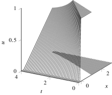

The code used to generate this figure is given in Appendix A.
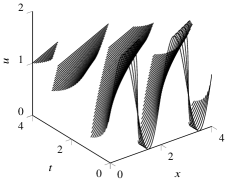
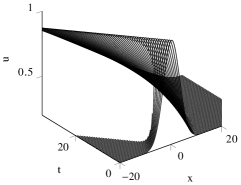
Example 2
We solve Burgers’ equation
using Implementation 1 and compare the result against the traditional method of characteristics for conservation laws. The maximum pointwise error (i.e., ) for the solution on a uniform grid of points covering the domain is . For this error calculation, the solution is computed in parallel using a MATLAB \mlttfamilyparfor loop at the rate of points per second (excluding the time for starting the parallel pool). Note, here we use MATLAB functions for \mlttfamilyg and \mlttfamilyG.
As in the previous example, we give the pointwise solution function to Chebfun and build piecewise continuous approximations to the solution shown in Figure 2.
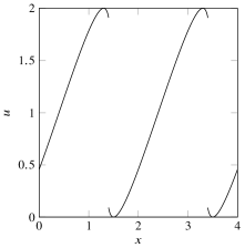
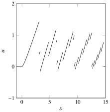
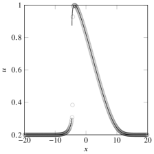
Example 3
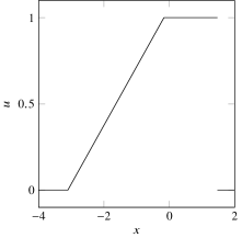
We solve Burgers’ equation with a compactly supported initial condition
which is an example of N-wave decay given in Chapter 11.5 of LeVeque [16]. As in the previous example, we give the pointwise solution function using Implementation 1 to Chebfun and build piecewise continuous approximations to the solution shown in Figure 3. For verification, this figure also presents a solution to this problem using a second-order Lax–Wendroff finite volume method with the van Leer limiter from Clawpack3 [5, 16] on a grid from of 1000 cells, which took seconds to compute to .
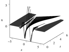
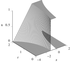
Example 4
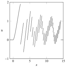
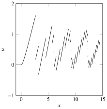
We solve Burgers’ equation with a compactly supported initial condition with many oscillations
which we use to demonstrate the ability of the proposed algorithm to find solutions with many shocks. As in the previous example, we give the pointwise solution function using Implementation 1 to Chebfun and build piecewise continuous approximations to the solution shown in Figure 4. Figure 5 further illustrates the complexity of the solution.

Example 5
For this example consider a LWR model for traffic flow, named after Lighthill and Whitham [17], Richards [25] and Richards [25],
| (27a) | |||||
| (27b) | |||||
| where | |||||
| (27c) | |||||
which is an example given in Chapter 11.1 of LeVeque [16]. Here is the density of the traffic flowing at a maximum speed . For this example we assume . The flux functions for this conservation law is concave upward and Algorithm 2 requires a conservation law with a convex downward flux function. Thus, we let which transforms the LWR model (27) to the convex conservation law
As in Example 3, we give the pointwise solution function using Implementation 1 to Chebfun and build piecewise continuous approximations to the solution shown in Figure 6. For verification, this figure also presents a solution to this problem using a second-order Lax–Wendroff finite volume method with the van Leer limiter from Clawpack3 [5, 16] on a grid from of 500 cells, which took seconds to reach .
Example 6
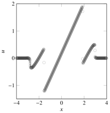
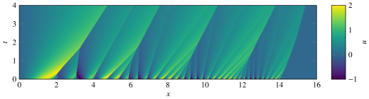
In this example we consider the following conservation law with a space-dependent flux function
| (28a) | |||||
| (28b) | |||||
Since the flux function is space-dependent, Algorithm 2 and the theory in Sections 3 and 4 do not apply. However, we can use Algorithm 1 to compute the unique minimum value solution. Some details required by the algorithm is given as follows. The associated Lagrangian is
and the Hamiltonian is
It is straightforward to derive relationship (8)
and the associated optimal control (9)
Given any point we want to compute . The Hamilton dynamics in (11) and (12) have the following form
The solution with the initial condition is
where is an arbitrary constant. Denote and by and , respectively, then we have
Solving for in terms of we have
and thus
In Step I of Algorithm 1, we solve the PMP (11) and (12). It is equivalent to finding that satisfies at least one set of the following conditions
| (29a) | ||||
| or | (29b) | |||
| or | (29c) | |||
| or | (29d) | |||
The optimal cost in Step II is
| (30) |
for where is a continuous function satisfying almost everywhere.
The solution of the conservation law (28) using Algorithm 2 is shown in Figure 7. The rarefaction and shock waves in the solution are clearly shown in the figure.
Example 7
The follow example is adopted from Zhang and Liu [30]. Consider the conservation law with a space-dependent flux
| (31a) | |||||
| (31b) | |||||
| (31c) | |||||
It can be shown that the problem has no shocks and the unique solution is
Again, we use Algorithm 1 to compute the unique minimum value solution. The associated Lagrangian is the Legendre transform of ,
The Hamiltonian is
and the optimal control satisfies
Then, it is straightforward to derive the PMP (11)
It is a two-point BVP of differential equations. For the purpose of testing a numerical implementation of Algorithm 1, we do not transform (32) into algebraic equations, although the differential equations can be explicitly solved. Instead, we use Chebfun to solve the BVP (32) as described in Birkisson and Driscoll [2]. Due to the uniqueness of solutions, Step II in Algorithm 1 is unnecessary. The Chebfun implementation of damped Newton method is used for the BVP solver with the standard termination criteria and the standard error tolerance of is used. The computation is carried out on a uniform grid of points in the region with a maximum absolute error of is observed.
6 Conclusions
Using optimal control theory, our study yields an algorithm and implementation for finding the minimum value solution of a scalar convex conservation laws, pointwise. It is proved that in the case of a space-independent flux function the minimum value solution is the entropy solution, thus providing a generalization of the Lax–Oleinik formula. Numerical results show good agreement of solutions from the proposed algorithm with that of analytical solutions and the finite volume method.
Appendix A Example using Implementation 1
As an example of using Implementation 1, we present the code used in Example 1 to generate Figure 1.
Here we give the point-wise solver \mlttfamilypdeccl to \mlttfamilychebfun to generate polynomial approximations of the solution, \mlttfamilyU, for various time instances, \mlttfamilyT.
Acknowledgements.
This work was supported in part by AFOSR, NRL, and DARPA. Thanks to Maurizio Falcone for his insights on fast Legendre–Fenchel transform.References
- che [2014] Chebfun guide. Pafnuty Publications, Oxford (2014). URL http://www.chebfun.org/docs/guide/
- Birkisson and Driscoll [2012] Birkisson, A., Driscoll, T.A.: Automatic Fréchet differentiation for the numerical solution of boundary-value problems. ACM Transactions on Mathematical Software 38(4), 26:1–26:29 (2012). doi:10.1145/2331130.2331134
- Boyd [2002] Boyd, J.P.: Computing zeros on a real interval through Chebyshev expansion and polynomial rootfinding 40(5), 1666–1682 (2002). doi:10.1137/s0036142901398325
- Chow et al. [2016] Chow, Y.T., Darbon, J., Osher, S., Yin, W.: Algorithm for overcoming the curse of dimensionality for certain non-convex Hamilton–Jacobi equations, projections and differential games. Tech. Rep. UCLA CAM 16-27, University of California, Los Angeles, Department of Mathematics, Group in Computational Applied Mathematics (2016). URL ftp://ftp.math.ucla.edu/pub/camreport/cam16-27.pdf. (revised August 2016)
- Clawpack Development Team [2016] Clawpack Development Team: Clawpack software (2016). URL http://www.clawpack.org. Version 5.3.1
- Corrias et al. [1995] Corrias, L., Falcone, M., Natalini, R.: Numerical schemes for conservation laws via Hamilton–Jacobi equations 64(210), 555 (1995). doi:10.1090/s0025-5718-1995-1265013-5
- Dafermos [2010] Dafermos, C.M.: Hyperbolic Conservation Laws in Continuum Physics. Grundlehren der mathematischen Wissenschaften, 3 edn. Springer Berlin Heidelberg (2010). doi:10.1007/978-3-642-04048-1
- Daganzo [2005] Daganzo, C.F.: A variational formulation of kinematic waves: Basic theory and complex boundary conditions. Transportation Research Part B: Methodological 39(2), 187–196 (2005). doi:10.1016/j.trb.2004.04.003
- Darbon and Osher [2016] Darbon, J., Osher, S.: Algorithms for overcoming the curse of dimensionality for certain Hamilton–Jacobi equations arising in control theory and elsewhere. ArXiv e-prints (arXiv:1605.01799) (2016). URL https://arxiv.org/abs/1605.01799
- Evans [2010] Evans, L.: Partial Differential Equations. American Mathematical Society (2010). doi:10.1090/gsm/019
- Good [1961] Good, I.J.: The colleague matrix, a Chebyshev analogue of the companion matrix 12(1), 61–68 (1961). doi:10.1093/qmath/12.1.61
- Kang and Wilcox [2015a] Kang, W., Wilcox, L.: A causality free computational method for HJB equations with application to rigid body satellites. In: AIAA Guidance, Navigation, and Control Conference, AIAA 2015-2009. American Institute of Aeronautics and Astronautics (2015a). doi:10.2514/6.2015-2009
- Kang and Wilcox [2015b] Kang, W., Wilcox, L.C.: Mitigating the curse of dimensionality: Sparse grid characteristics method for optimal feedback control and HJB equations. ArXiv e-prints (arXiv:1507.04769) (2015b). URL https://arxiv.org/abs/1507.04769
- Lax [1973] Lax, P.D.: Hyperbolic Systems of Conservation Laws and the Mathematical Theory of Shock Waves. Society for Industrial & Applied Mathematics (1973). doi:10.1137/1.9781611970562
- LeVeque [1992] LeVeque, R.J.: Numerical Methods for Conservation Laws. Springer Science + Business Media (1992). doi:10.1007/978-3-0348-8629-1
- LeVeque [2002] LeVeque, R.J.: Finite Volume Methods for Hyperbolic Problems. Cambridge University Press (2002). doi:10.1017/cbo9780511791253
- Lighthill and Whitham [1955] Lighthill, M.J., Whitham, G.B.: On kinematic waves. II. A theory of traffic flow on long crowded roads. Proceedings of the Royal Society A: Mathematical, Physical and Engineering Sciences 229(1178), 317–0345 (1955). doi:10.1098/rspa.1955.0089
- Luke [1972] Luke, J.C.: Mathematical models for landform evolution. Journal of Geophysical Research 77(14), 2460–2464 (1972). doi:10.1029/jb077i014p02460
- Newell [1993] Newell, G.F.: A simplified theory of kinematic waves in highway traffic, part I: General theory. Transportation Research Part B: Methodological 27(4), 281–287 (1993). doi:10.1016/0191-2615(93)90038-c
- Osher and Fedkiw [2003] Osher, S., Fedkiw, R.: Level Set Methods and Dynamic Implicit Surfaces. Springer-Verlag, New York (2003). doi:10.1007/978-0-387-22746-7
- Osher and Sethian [1988] Osher, S., Sethian, J.A.: Fronts propagating with curvature-dependent speed: Algorithms based on Hamilton–Jacobi formulations. Journal of Computational Physics 79(1), 12–49 (1988). doi:10.1016/0021-9991(88)90002-2
- Osher and Shu [1991] Osher, S., Shu, C.W.: High-order essentially nonoscillatory schemes for Hamilton–Jacobi equations. SIAM Journal on Numerical Analysis 28(4), 907–922 (1991). doi:10.1137/0728049
- Pachón et al. [2009] Pachón, R., Platte, R.B., Trefethen, L.N.: Piecewise-smooth chebfuns 30(4), 898–916 (2009). doi:10.1093/imanum/drp008
- Qiu and Shu [2008] Qiu, J.M., Shu, C.W.: Convergence of Godunov-type schemes for scalar conservation laws under large time steps. SIAM Journal on Numerical Analysis 46(5), 2211–2237 (2008). doi:10.1137/060657911
- Richards [1956] Richards, P.I.: Shock waves on the highway. Operations Research 4(1), 42–51 (1956). doi:10.1287/opre.4.1.42
- Specht [1957] Specht, W.: Die lage der nullstellen eines polynoms. III 16(5-6), 369–389 (1957). doi:10.1002/mana.19570160509
- The MathWorks, Inc. [2014] The MathWorks, Inc.: MATLAB R2014b. Natick, Massachusetts, United States (2014)
- Trefethen [2012] Trefethen, L.N.: Approximation Theory and Approximation Practice. Society for Industrial and Applied Mathematics, Philadelphia, PA, USA (2012). URL http://www.chebfun.org/ATAP/
- Wright et al. [2015] Wright, G.B., Javed, M., Montanelli, H., Trefethen, L.N.: Extension of Chebfun to periodic functions 37(5), C554–C573 (2015). doi:10.1137/141001007
- Zhang and Liu [2005] Zhang, P., Liu, R.X.: Hyperbolic conservation laws with space-dependent fluxes: II. General study of numerical fluxes 176(1), 105–129 (2005). doi:10.1016/j.cam.2004.07.005