Monotone Retargeting for Unsupervised Rank Aggregation with Object Features

Abstract

Learning the true ordering between objects by aggregating a set of expert opinion rank order lists is an important and ubiquitous problem in many applications ranging from social choice theory to natural language processing and search aggregation. We study the problem of unsupervised rank aggregation where no ground truth ordering information in available, neither about the true preference ordering between any set of objects nor about the quality of individual rank lists. Aggregating the often inconsistent and poor quality rank lists in such an unsupervised manner is a highly challenging problem, and standard consensus-based methods are often ill-defined, and difficult to solve. In this manuscript we propose a novel framework to bypass these issues by using object attributes to augment the standard rank aggregation framework. We design algorithms that learn joint models on both rank lists and object features to obtain an aggregated rank ordering that is more accurate and robust, and also helps weed out rank lists of dubious validity. We validate our techniques on synthetic datasets where our algorithm is able to estimate the true rank ordering even when the rank lists are corrupted. Experiments on three real datasets, MQ2008, MQ2008 and OHSUMED, show that using object features can result in significant improvement in performance over existing rank aggregation methods that do not use object information. Furthermore, when at least some of the rank lists are of high quality, our methods are able to effectively exploit their high expertise to output an aggregated rank ordering of great accuracy.

1 Introduction

Learning preference orderings among objects is a common problem in many modern applications including web search, document retrieval, collaborative filtering and recommendation systems. Rank aggregation is a version of this problem that appears in areas ranging from voting and social choice theory [35], to meta search and search aggregation [25] to ensemble methods for combining classifiers [21].

We focus on the problem of unsupervised rank aggregation [22, 23] in this manuscript. The standard setup consists of a set of $n$ items or objects to be ranked, and a set of $p$ ranking lists from “experts” (possibly inconsistent, and of varying levels of expertise and credibility) containing rank scores or relevance scores for all or a subset of the $n$ items, and the objective is to combine the lists from different experts and obtain a consensus rank order over the set of items. Note that this setup is different from supervised rank aggregation [28, 30, 37] or semi-supervised rank aggregation [10, 15] where, in addition to the rank lists, we also have ground truth rank orderings between at least a subset of the objects to be ranked (for example, ground truth rank orderings supplied by high expertise human annotators or subject matter experts, that can then be used as training data). In contrast, in the unsupervised setup, we are only given access to rank lists without any information about the quality of each list, or any ground truth rank order between objects.

A related but very distinct problem that also looks at ordering among items is learning to rank or LETOR [17, 14, 9], which tries to learn ranking functions over objects given training data with known rank scores or pairwise preference information. Standard methods for LETOR model the rank scores or orderings as a function of features associated with the objects.

The difference between LETOR and unsupervised rank aggregation is two-fold. First, unlike the latter, LETOR is supervised and has access to training data. Second, while LETOR models rank scores as functions of object features, existing rank aggregation methods are completely agnostic to the properties of the objects being ranked, even when such information is available, for example in the case of meta-search, search aggregation, or ensemble methods over learning agents[25, 21]. As a result, rank aggregation is significantly more challenging to tackle as compared to LETOR, or supervised/semi-supervised methods in general.

Without access to any information about true preference ordering among objects, the standard rank aggregation problem becomes a hard combinatorial problem, and often rife with paradoxes [4]. Rule based approaches like Borda winner [38], Condorcet winner [8], etc., are commonly used, but many of these rules are incompatible with each other [35]. Alternative approaches learn consensus orderings by minimising “disagreements” or distance-like metrics among the rank scores or preference orderings specified by the ranked lists from experts [19, 20]. This approach runs into the problem that for many of the commonly used distance metrics, the corresponding optimisation problem is NP-Hard [11].

Indeed, without additional information, one cannot form an incontrovertible definition for “consensus” and “disagreement” between rank scores, or even decide on the metric to be used to find the consensus rank ordering. Moreover, these methods are excessively dependent on the assumption that the experts are reliable and competent. Spurious rank order lists or even the presence of noise in the ranked lists can significantly deteriorate the performance of most standard methods used for rank aggregation.

1.1 Using Object Information

The absence of supervision reduces rank aggregation to a problem of choosing between competing heuristics. But obtaining even partial ground truth can be expensive and time consuming and often requires the involvement of dedicated human experts as annotators.

This manuscript introduces a novel rank aggregation framework that mitigates the handicaps of unsupervised rank aggregation by using information about object attributes to augment standard approaches and aid the recovery of the “true” rank order. This is in contrast to existing methods which are “blind” in the sense that they are completely agnostic to the properties of the objects themselves.

Our key contributions are summarised as follows-

1. To the best of our knowledge, we are the first to use object information to aid the rank aggregation problem. We introduce a novel framework that combines information from rank scores and object features to learn a consensus ordering over a set of items.

2. We formulate the rank aggregation problem using isotonically coupled models over expert lists and object features to model rank scores, and describe a solution algorithm to estimate the true ordering that involves alternate but interdependent iterations between a LETOR step and a rank aggregation step, each of which is separately a simple convex optimisation problem with monotonicity constraints.

3. We evaluate our framework with experiments on synthetic data where, unlike existing methods, our algorithm is able to reconstruct the true rank ordering exactly given corrupted rank lists. We also demonstrate our methods on three real datasets, where our algorithm significantly outperforms existing rank aggregation techniques that do not use object information.

We note that even though our framework uses LETOR inspired methods, our formulation is still an unsupervised learning algorithm since we do not assume access to any full or partial ground truth rank order or pairwise preferences, or even information about the quality of any rank lists.

1.2 Related Work

In light of the difficulties inherent in the rank aggregation problem, most of the commonly used rank aggregation applications apply heuristic based techniques ranging from classical methods for vote counting, combination methods involving linear and non-linear functions, and more recent approaches involving Markov Chain Monte Carlo simulations.

The Borda Count [38] is the traditional vote counting procedure that uses positional information as opposed to rank scores. The procedure orders the candidates (items) by the number of candidates ranked lower than them, averaged over the set of voters (expert lists).

Combination methods [12, 26] work on explicit relevance scores provided by experts and include various linear combinations like CombSUM, CombMNZ and CombANZ as well as non-linear methods like CombMIN and CombMAX. It has been seen [26, 5] that out of the three linear combination methods, CombMNZ has the best performance. If all items have been retrieved by all expert lists, all three methods give the same final ranking.

Among non-linear methods [26, 12], CombMIN and CombMAX respectively rank the items on the minimum and maximum scores received across the lists provided by experts.

More recent work [11] on rank aggregation have introduced MCMC based methods. The basic idea is to use the items to be ranked as states of a Markov Chain and define the transition probability of switching from one state (item) to another, based on the relative scores or preference values of the corresponding items across rank lists. Four different Markov Chain constructions (MC1, MC2, MC3, MC4) have been described in [11] that use different heuristics to construct the transition probability matrix. The final ranking of the items is defined by the stationary distribution across the items defined by the states of the Markov Chain.

Note On Notation: The vector $\mathbf{r}$ is said to be in increasing order if $r_{i}\leq r_{j}$ whenever $i\leq j$. The set of all such vectors in $\mathbb{R}^{n}$ is denoted with a subscripted downward pointing arrow as $\mathbb{R}^{n}_{\downarrow}$. Two vectors $\mathbf{r}$ and $\mathbf{z}$ are said to be isotonic, $\mathbf{r\sim_{\downarrow}z}$, if $r_{i}\geq r_{j}$ if and only if $z_{i}\geq z_{j}$ for all $i,j$.

2 Problem Setup

Let $\mathcal{V}$ be a set of distinct items and $\mathcal{Q}=\{\mathbf{q}_{1},\cdots,\mathbf{q}_{|\mathcal{Q}|}\}$ be a set of queries. Each query $\mathbf{q}$ is associated with a set of items $\mathbf{V}_{\mathbf{q}}\subset\mathcal{V}$. For simplicity and with no loss in generality, we consider the case of a single query over a set of $n$ items, and drop the notation $\mathbf{q}$ from all subsequent notation.

Suppose the true rank ordering over $n$ items is given by a vector ${\bm{\rho}}^{*}\in\mathbb{R}^{n}$. In search aggregation, for example, ${\bm{\rho}}^{*}$ could be true relevance scores as annotated by a human subject matter expert. With slight abuse of notation, we shall overload ${\bm{\rho}}^{*}$ to denote both a rank score as well as a rank ordering (permutation) defined by the rank score vector.

In the standard rank aggregation setup, we are given access to rank lists by a set of $p$ experts, each of whom assert a rank ordering or relevance score judgement over the entire set of items in $\mathbf{V}$. Suppose that the relevance score vector for the $k^{th}$ expert is $\mathbf{r}^{k}\in\mathbb{R}^{n}$, where a higher score indicates a higher relevance for the item. We aggregate all relevance score lists as columns of the rank list matrix $\mathbf{R}=[\mathbf{r}^{1};\mathbf{r}^{2};\cdots\mathbf{r}^{p}]\in\mathbb{R}^{n\times p}$.

In unsupervised rank aggregation, the true ordering ${\bm{\rho}}^{*}$ is not known, even among a partial subset of objects. However, it is assumed that at least some of the rank lists in $\mathbf{R}$ are generated using ${\bm{\rho}}^{*}$ (perhaps from noisy or corrupted versions of ${\bm{\rho}}^{*}$) and standard rank aggregation methods try to recover ${\bm{\rho}}^{*}$ by learning a model that maps $\mathbf{R}$ to a vector $\overline{\mathbf{r}}$ that is isotonic with ${\bm{\rho}}^{*}$ (e.g. Borda Count, combination methods, etc. see section (1.2)).

In this manuscript we try to overcome the limitations of unsupervised rank aggregation as described in section (1) by augmenting our setup with object features, which are often available in applications like meta-search, IR, etc. Suppose for the set of items $\mathcal{V}=\{V_{1},V_{2},\cdots V_{n}\}$, each item $V_{i}$ can be represented by a $d$-dimensional feature vector $\mathbf{x}_{i}\in\mathbb{R}^{d}$. We collect all these item feature vectors to form rows of the feature matrix $\mathbf{X}\in\mathbb{R}^{n\times d}$. The consensus rank ordering is then obtained using information from both $\mathbf{R}$ and $\mathbf{X}$.

To motivate our approach, consider the standard supervised LETOR framework which has access to both $\mathbf{X}$ as well as ${\bm{\rho}}^{*}$. Popular LETOR methods [14, 9, 27] proceed by learning a model that maps $\mathbf{X}$ to a rank score vector $\overline{\mathbf{z}}$ that is isotonic with ${\bm{\rho}}^{*}$. Similarly, many standard methods for supervised rank aggregation [28, 30] proceed by learning a model that maps $\mathbf{R}$ to a vector that agrees with available information about ${\bm{\rho}}^{*}$.

In contrast, ${\bm{\rho}}^{*}$ is completely unknown in unsupervised rank aggregation. The key idea for our method is that while we do not have explicit access to ${\bm{\rho}}^{*}$, both $\mathbf{X}$ and $\mathbf{R}$ are implicitly tied together by ${\bm{\rho}}^{*}$, and this implicit association can be exploited to recover ${\bm{\rho}}^{*}$ by jointly modelling the mappings that can be learned from $\mathbf{X}$ and $\mathbf{R}$ respectively.

To our knowledge, while object attributes are commonly available for many rank aggregation setups (e.g. meta-search or search aggregation), none of the existing rank aggregation methods exploit them sufficiently. As a first work, we explore the use of generalised linear models or GLMs [29] as our modeling framework since they are a large class of models that subsume many standard modeling frameworks (e.g. Gaussian or Poisson regression), and are widely used for many applications across a wide variety of domains. In particular, GLMs have found extensive usage in both LETOR [3, 1] as well as most rank aggregation methods [38, 12, 26].

3 Rank Aggregation with Object Features

GLM’s model the target variable (in this case, rank score) as a linear function of the feature variables, monotonically transformed via a monotonic link function. We assume that the true rank ordering ${\bm{\rho}}^{*}$ can be modeled as a monotonically transformed linear combination of the rank order lists $\mathbf{R}\in\mathbb{R}^{n\times p}$ by the experts, that is, ${\bm{\rho}}^{*}\sim_{\downarrow}\mathbf{R}{\bm{\beta}}^{*}$ for some ${\bm{\beta}}^{*}\in\mathbb{R}^{p}$. Even without the monotonic transformation, this setup subsumes standard score fusion algorithms, eg. see [16, 12], and also the Borda-Count and weighted Borda-Fuse [38, 35] if the rank scores are defined as the number of items ranked below a particular item. This setup can also effectively handle the case when some of the ranked lists are of dubious validity– such rank lists can simply be assigned zero weight and discarded by the model.

Similarly, we also assume that the true rank score vector ${\bm{\rho}}^{*}$ is isotonic to a monotonically transformed linear function of the object features, that is, ${\bm{\rho}}^{*}\sim_{\downarrow}\mathbf{X}{\bm{\omega}}^{*}$ for some ${\bm{\omega}}^{*}\in\mathbf{R}^{d}$. This is a standard assumption for many ranking problems that model the rank function using a generalised linear model (see [3, 1] and references).

The objective now is to estimate ${\bm{\beta}}^{*}$ and ${\bm{\omega}}^{*}$ by joint modelling of $\mathbf{X}{\bm{\omega}}^{*}$ and $\mathbf{R}{\bm{\beta}}^{*}$ to estimate $\omega^{*}$ and ${\bm{\beta}}^{*}$ by minimising an appropriate distance-like cost function. Clearly, standard cost functions like square loss may not make sense in every context (for example, when the domain is binary, or integer valued, or categorical), therefore we present our techniques for a much more general class of cost functions called Bregman divergences, which are distance-like functions intimately associated with GLM’s and include many standard and commonly used loss functions like square loss, KL-Divergence, Generalised I-Divergence, etc.

Bregman Divergences: The matching loss functions associated with learning GLM parameters are distance-like functions called Bregman divergences, which are generalisations of square loss. Bregman Divergences are always defined on a convex function ${\bm{\phi}}(\cdot)$, where the particular convex function used depends on the particular GLM model used (see [6]). For any two vectors $\mathbf{y}$ and $\mathbf{x}$, the Bregman divergence $D_{\bm{\phi}}(\cdot\|\cdot)$ between the vectors corresponding to the function ${\bm{\phi}}$ is defined as

$$D_{\bm{\phi}}\left(\mathbf{y}\|\mathbf{x}\right)\triangleq{\bm{\phi}}(\mathbf{y})-{\bm{\phi}}(\mathbf{x})-\langle\nabla{\bm{\phi}}(\mathbf{x}),\mathbf{y}-\mathbf{x}\rangle$$

A more detailed description of Bregman Divergences is deferred to Appendix (A), see also [6] for a rigorous exposition on the relationship between GLM’s and Bregman Divergences. In particular, for our work we use the fact that parameter estimation in a GLM with given object features $\mathbf{X}$ and known target variable $\mathbf{z}$ is equivalent to finding the minimiser ${\bm{\omega}}^{*}$ for $D_{\bm{\phi}}\left(\mathbf{z}\|(\nabla{\phi})^{-1}(\mathbf{X}{\bm{\omega}})\right)$ as,

$${\bm{\omega}}^{*}=\text{arg}\min_{{\bm{\omega}}}D_{{\bm{\phi}}}\left({\mathbf{z}}\|(\nabla{\phi})^{-1}({\mathbf{X}{\bm{\omega}}})\right)$$ (1)

where ${\bm{\phi}}(\cdot)$ is the convex function associated with the specific GLM used– for a Gaussian model or equivalently square loss, for example, ${\bm{\phi}}$ is the identity function (see [6]).

Bregman Divergences are always non-negative $D_{\bm{\phi}}(\cdot\|\cdot)\geq 0$, and by definition, $D_{{\bm{\phi}}}\left({\mathbf{z}}\|(\nabla{\phi})^{-1}({\mathbf{X}{\bm{\omega}}})\right)$ is separately convex in $\mathbf{z}$ as well as in ${\bm{\omega}}$. Many standard distance-like functions like Square loss, Kullback-Leibler (KL) divergence and Generalised I-divergence can be written as members of this family for their corresponding ${\bm{\phi}}$. For succinctness, we shall henceforth denote $D_{{\bm{\phi}}}\left({\mathbf{z}}\|(\nabla{\phi})^{-1}({\mathbf{X}{\bm{\omega}}})\right)$ simply as $D_{\bm{\phi}}(\mathbf{z}\|\mathbf{X}{\bm{\omega}})$.

3.1 Cost Function

Following the discussion on using Bregman divergences as the loss function for estimating ${\bm{\omega}}^{*}$ and ${\bm{\beta}}^{*}$, it is tempting to use $\mathbf{R}{\bm{\beta}}$ as the target variable and $\mathbf{X}{\bm{\omega}}$ as the feature map, and write the joint optimisation framework as follows:

$${\bm{\beta}}^{*},{\bm{\omega}}^{*}=\text{arg}\min_{{\bm{\beta}},{\bm{\omega}}}D_{{\bm{\phi}}}\left({\mathbf{R}{\bm{\beta}}}\|{\mathbf{X}{\bm{\omega}}}\right)$$ (2)

Alternatively, the order of arguments $(\mathbf{R}{\bm{\beta}},\mathbf{X}{\bm{\omega}})$ can be reversed. However, both these formulations are deficient in their modelling capacity since they force a coupling between the domain of $\mathbf{X}$ and the domain of $\mathbf{R}$. In particular, while $\mathbf{X}$ is often real valued, $\mathbf{R}$ can often be integer valued or binary valued, or even categorical with partial ordering and the same ${\bm{\phi}}$ may not make sense for both. Moreover, this does not take into account the more general assumption that the true ordering need only be isotonic to the two linear functions, that is $\mathbf{R}{\bm{\beta}}\sim_{\downarrow}\mathbf{X}{\bm{\omega}}$, but exact equality may be an unnecessarily strong and superfluous constraint. Incorporating monotonic invariance between $\mathbf{R}{\bm{\beta}}$ and $\mathbf{X}{\bm{\omega}}$ is a challenging problem in the above formulation.

A far better alternative scheme that bypasses all these issues involves decoupling the cost function into two parts- one involving the rank scores by experts and one involving the object features.

3.1.1 Decoupled Cost Function

Consider $\overline{\mathbf{r}}\in\mathbb{R}^{n}$ as the rank score vector to be fitted against a linear function of the rank score matrix $\mathbf{R}$. This part of the decoupled cost function therefore consists of the term $D_{{\bm{\phi}}_{r}}\left({\overline{\mathbf{r}}}\|{\mathbf{R}{\bm{\beta}}}\right)$ for an appropriate ${\bm{\phi}}_{r}$. Since we consider all rank score vectors that invoke the same ordering among items to be equivalent, we shall be learning $\overline{\mathbf{r}}$ across all monotonic transformations to incorporate invariance across isotonic vectors in our formulation.

Similarly, suppose $\overline{\mathbf{z}}\in\mathbb{R}^{n}$ is the rank score vector obtained as the linear function of object features. Correspondingly, this part of the cost function becomes $D_{{\bm{\phi}}_{z}}\left({\overline{\mathbf{z}}}\|{\mathbf{X}{\bm{\beta}}}\right)$ for an appropriate ${\bm{\phi}}_{z}$. Along the same lines as above, we learn $\overline{\mathbf{z}}$ across all monotonic transformations.

Therefore, the full cost function becomes

$$\mathcal{C}(\mathbf{r},{\bm{\beta}},\overline{\mathbf{z}},{\bm{\omega}})=D_{{\bm{\phi}}_{r}}\left({\mathbf{r}}\|{\mathbf{R}{\bm{\beta}}}\right)+\lambda D_{{\bm{\phi}}_{z}}\left({\overline{\mathbf{z}}}\|{\mathbf{X}{\bm{\omega}}}\right)$$ (3)

to be minimised over $\overline{\mathbf{r}},{\bm{\beta}},\overline{\mathbf{z}},{\bm{\omega}}$. To retain the isotonicity relationship between the linear functions $\mathbf{R}{\bm{\beta}}$ and $\mathbf{X}{\bm{\omega}}$, we add the constraint $\overline{\mathbf{r}}\sim_{\downarrow}\overline{\mathbf{z}}$. The overall optimisation problem therefore becomes

$$\underset{\overline{\mathbf{r}},{\bm{\beta}},\overline{\mathbf{z}},{\bm{\omega}}}{\text{min}} \ \ D_{{\bm{\phi}}_{r}}\left({\overline{\mathbf{r}}}\|{\mathbf{R}{\bm{\beta}}}\right)+\lambda D_{{\bm{\phi}}_{z}}\left({\overline{\mathbf{z}}}\|{\mathbf{X}{\bm{\omega}}}\right)$$ (4)

s.t. $$\ \ \overline{\mathbf{r}}\sim_{\downarrow}\overline{\mathbf{z}}$$

Choice of divergence functions ${\bm{\phi}}_{r}$ and ${\bm{\phi}}_{z}$ depends on the domain (real valued, integer, etc.) and the modeling assumptions used on $\overline{\mathbf{r}}$ and $\overline{\mathbf{z}}$, a discussion on learning the appropriate ${\bm{\phi}}$ has been detailed in [2]. We shall see later that our optimisation framework involves steps that are invariant to the $\lambda$ value chosen, so we use $\lambda=1$ for simplicity.

4 Monotonically Retargeted Rank Aggregation

Equation ((4)) is an optimisation problem of a function that is separately convex in its arguments, but over a non-convex set. Joint optimisation over all variables simultaneously is difficult, therefore we divide the variables into two disjoint sets and perform alternating minimisation over each set of variables separately. Nevertheless, because of the monotonic invariance of the isotonicity constraint we need to perform each optimisation step over all monotonic transformations of the vectors $\overline{\mathbf{r}}$ and $\overline{\mathbf{z}}$, which is a very difficult problem in general. However, it turns out that the setup becomes relatively easy to handle by using a technique called monotone retargeting used in supervised learning to rank problems.

Monotone Retargeting or MR [3] is a LETOR technique that uses object attributes $\mathbf{X}$ and known rank score vector ${\bm{\rho}}^{*}$ and learns a model that finds the best mapping from $\mathbf{X}$ over all possible monotonic transformations $\mathbf{z}$ of the rank score vector ${\bm{\rho}}^{*}$. The specific optimisation problem that MR handles in the case of Bregman Divergences (i.e., using GLM’s) is the following:

$$\underset{\mathbf{z},{\bm{\omega}}}{\text{min}} D_{\bm{\phi}}\left(\mathbf{z}\|(\nabla{\phi})^{-1}(\mathbf{X{\bm{\omega}}})\right)$$ (5)

s.t. $$\mathbf{z}\sim_{\downarrow}{\bm{\rho}}^{*}$$

To impose strict ordering constraints and to avoid degenerate solutions, a variation of MR called Margin Equipped Monotone Retargeting or MEMR was introduced in [1] that uses margin constraints on $\mathbf{z}$ together with ordering constraints defined by ${\bm{\rho}}^{*}$. A detailed description of MR and MEMR is given in Appendices (B) and (C) respectively. The steps used in the exact optimisation algorithm for MR is summarised as Algorithm (1).

MR is a versatile framework that has found usage outside of the traditional supervised ranking application it was designed for. In particular, versions of this framework have been used for collaborative filtering for recommendation systems [24], and learning generalised linear models from aggregated data [7]. In this manuscript we apply this framework to the problem of rank aggregation.

Algorithm 1 LETOR with Monotone Retargeting

1:procedure MR(${\bm{\phi}},\mathbf{X},{\bm{\rho}}^{*}$)

2:     Initialise ${\bm{\omega}},\overline{\mathbf{z}}$

3:     while not converged do

4:         Solve for $\overline{\mathbf{z}}^{+}$ using PAV

$$\overline{\mathbf{z}}^{+}=\text{arg}\min_{\overline{\mathbf{z}}\sim_{\downarrow}{\bm{\rho}}^{*}}D_{{\bm{\phi}}}\left({\overline{\mathbf{z}}}\|{\mathbf{X}{\bm{\omega}}}\right)\vspace*{-0.1cm}$$

5:         Solve for ${\bm{\omega}}^{+}$ a std GLM param estimation

$$\ \ \ {\bm{\omega}}^{+}=\text{arg}\min_{{\bm{\omega}}}D_{{\bm{\phi}}}\left({\overline{\mathbf{z}}^{+}}\|{\mathbf{X}{\bm{\omega}}}\right)\vspace*{-0.15cm}$$

6:         Update variables $(\overline{\mathbf{z}},{\bm{\omega}})=(\overline{\mathbf{z}}^{+},{\bm{\omega}}^{+})$

7:     end while

8:     return $\overline{\mathbf{z}},{\bm{\omega}}$

9:end procedure

Consider the set of variables $\Upsilon=(\overline{\mathbf{r}},{\bm{\beta}},\overline{\mathbf{z}},{\bm{\omega}})$ divided into two sets of variables $\Upsilon_{\mathbf{r}}=(\overline{\mathbf{r}},{\bm{\beta}})$ and $\Upsilon_{\mathbf{z}}=(\overline{\mathbf{z}},{\bm{\omega}})$. After initialisation (which can be done by using any preferred rank aggregation algorithm), the algorithm proceeds in two alternating steps. First, keeping $\Upsilon_{\mathbf{z}}$ fixed, the optimisation problem over $\Upsilon_{\mathbf{r}}$ becomes

$$\underset{\overline{\mathbf{r}},{\bm{\beta}}}{\text{min}} D_{{\bm{\phi}}_{r}}\left({\overline{\mathbf{r}}}\|{\mathbf{R}{\bm{\beta}}}\right)$$ (6)

s.t. $$\overline{\mathbf{r}}\sim_{\downarrow}\overline{\mathbf{z}}$$

Similarly, keeping $\Upsilon_{\mathbf{r}}$ fixed, the optimisation problem over $\Upsilon_{\mathbf{z}}$ becomes

$$\underset{\overline{\mathbf{z}},{\bm{\omega}}}{\text{min}} D_{{\bm{\phi}}_{z}}\left({\overline{\mathbf{z}}}\|{\mathbf{X}{\bm{\omega}}}\right)$$ (7)

s.t. $$\overline{\mathbf{z}}\sim_{\downarrow}\overline{\mathbf{r}}$$

At face value, because of the common isotonicity constraint $\overline{\mathbf{r}}\sim_{\downarrow}\overline{\mathbf{z}}$ applied to both steps of the optimisation problem, it may seem the algorithm will remain perpetually stuck to the rank ordering defined by the initialisation of $\overline{\mathbf{r}}$ or $\overline{\mathbf{z}}$. However, this does not happen because at alternate steps, the $\overline{\mathbf{z}}$ or $\overline{\mathbf{r}}$ that define the isotonicity constraint can be partially ordered rather than totally ordered. This enables the algorithm to freely move between permutations at successive steps. A detailed discussion of this phenomenon is provided in Section (5.2).

Algorithm 2 Rank Aggregation with Object Features

1:procedure MR-RankAgg(${\bm{\phi}}_{r},\mathbf{R},{\bm{\phi}}_{z},\mathbf{X}$)

2:     Initialise $\overline{\mathbf{r}},{\bm{\beta}},\overline{\mathbf{z}},{\bm{\omega}}$

3:     while not converged do

4:         $\overline{\mathbf{z}}^{+},{\bm{\omega}}^{+}=\text{{MR}}({\bm{\phi}}_{z},\mathbf{X},\overline{\mathbf{r}})$ LETOR-step

5:         $\overline{\mathbf{r}}^{+},{\bm{\beta}}^{+}=\text{{MR}}({\bm{\phi}}_{r},\mathbf{R},\overline{\mathbf{z}}^{+})$ Rank-Agg step

6:         Update all variables

$$(\overline{\mathbf{r}},{\bm{\beta}},\overline{\mathbf{z}},{\bm{\omega}})\leftarrow(\overline{\mathbf{r}}^{+},{\bm{\beta}}^{+},\overline{\mathbf{z}}^{+},{\bm{\omega}}^{+})\vspace*{-0.15cm}$$

7:     end while

8:     return $(\overline{\mathbf{r}},{\bm{\beta}},\overline{\mathbf{z}},{\bm{\omega}})$

9:end procedure

Individually, both equations ((6)) and ((7)) are standalone instances of MR and inherit all the desirable properties of the algorithm as detailed in [3, 1]. The two main steps of the algorithm have a nice interpretation– equation ((6)) is equivalent to MR(${\bm{\phi}}_{r},\mathbf{R},\overline{\mathbf{z}}$) and is analogous to a LETOR step, while equation ((7)) is equivalent to MR(${\bm{\phi}}_{z},\mathbf{X},\overline{\mathbf{r}}$) and is analogous to a rank aggregation step. The steps used in the overall optimisation are summarised in Algorithm (2).

Convergence and Efficiency: Algorithm (2) uses alternating minimisation on a non-negative cost function, therefore the algorithm always converges to a stationary point. Each iteration involves the MR procedure detailed in Algorithm (1), which can be implemented very efficiently in practice (see [1]). In particular, the PAV step has been implemented in $\Theta(n)$ (see references in [36]). Both the PAV step and the GLM-solver step have been extensively studied, and fast off-the-shelf implementations are readily available.

4.1 Margin Equipped Version

To avoid certain kinds of degeneracies (see [1]), MEMR uses a formulation that enforces an $\epsilon$-margin between the relevance scores between any two items adjacent to each other in the learned rank score vector $\mathbf{z}$. We can formulate a margin-equipped version for our methods as well, however the MEMR scheme cannot be used directly. As we discuss in section (5.2), one of the salient desiderata of our formulation is to be able to move between rank orderings at every step of the algorithm, which is achieved by using the partial orderings for $\overline{\mathbf{r}}$ or $\mathbf{z}$ generated by the optimisation algorithm at the end of each iteration. Imposing a strict ordering would make that no longer possible.

In fact, in most cases a strict ordering is unnecessary– to avoid degenerate solutions as in [1], it is sufficient to enforce a margin only between the maximum and the minimum rank score. That is, the constraint we shall use, say on $\overline{\mathbf{r}}$, would be of the form $\overline{\mathbf{r}}^{(max)}-\overline{\mathbf{r}}^{(min)}>\epsilon$ for some $\epsilon>0$. While this is a non-linear, non-convex condition in general, within the constraint set $\overline{\mathbf{r}}\sim_{\downarrow}\overline{\mathbf{z}}$, this becomes a simple half-space constraint since the indices for maximum and minimum in $\overline{\mathbf{r}}$ are already specified by the ordering defined by $\overline{\mathbf{z}}$. A similar margin constraint can be applied to $\overline{\mathbf{z}}$ as well.

5 Discussion

5.1 Regularisation

Adding a convex regularisation term (especially on the GLM parameters ${\bm{\beta}}$ and ${\bm{\omega}}$) in equation (4) can have many useful effects while retaining convexity properties in the optimisation problem. In particular, suppose we know that some of the rank order lists are spurious or generated by sources of dubious expertise. In such a case, sparsity promoting methods like LASSO regularisation on ${\bm{\beta}}$ may help weed out the spurious rank lists by enforcing sparsity. A similar argument can also be made for adding sparsity boosting regularisers on ${\bm{\omega}}$ to weed out spurious features.

5.2 Moving between permutations

One of the key desiderata of our algorithm is that the $\overline{\mathbf{r}}$ or $\overline{\mathbf{z}}$ in intermediate steps should be free to move between permutations, so that the final aggregated output for rank order does not get influenced too heavily by the initialisation. This is accomplished by our algorithm in the following manner.

The update step for $\overline{\mathbf{z}}$ in the MR Algorithm (1) involves a pool-adjacent-violator (PAV) smoothing operation, which has the property that if the ordering constraint on $\overline{\mathbf{z}}$ does not match the ordering of the right hand side $\mathbf{X}{\bm{\beta}}$, the final output would be a partially ordered $\overline{\mathbf{z}}$. Suppose at time $t$, we start with some total ordering ${\bm{\rho}}_{0}$ on $\overline{\mathbf{z}}$ and $\overline{\mathbf{r}}$, and after step ((4)) in Algorithm (2) we end up with a $\overline{\mathbf{z}}^{+}$ which is consistent with ${\bm{\rho}}_{0}$ but is partially ordered. When such a partially ordered $\overline{\mathbf{z}}^{+}$ is used as an input for estimating $\overline{\mathbf{r}}^{+}$ at step ((5)) of Algorithm (2), the final output for $\overline{\mathbf{r}}^{+}$ may have a total ordering ${\bm{\rho}}_{1}$ which is consistent with the partial ordering specified by $\overline{\mathbf{z}}^{+}$, but not necessarily consistent with the total ordering ${\bm{\rho}}_{0}$. Therefore, between time $t$ and time $t+1$, the algorithm ends up moving from the ordering ${\bm{\rho}}_{0}$ to the ordering ${\bm{\rho}}_{1}$.

Subsequently, we shall show with experiments on synthetic data that this is indeed the case. Starting from an initialisation that does not reflect the true ordering, the $\overline{\mathbf{r}}$ and $\overline{\mathbf{z}}$ obtained by our algorithm are allowed to move between permutations till they converge to a stationary point corresponding to the exact ordering.

5.3 Extensions

While the methods outlined in this manuscript used GLM’s and Bregman Divergences, our formulation is much more general. Specifically, techniques like MR were used to illustrate one of many possible ways of jointly modeling rank scores with object features, and other methods from the supervised LETOR or rank aggregation literature can be easily incorporated into our framework by changing the cost function and optimisation algorithm. Similarly, our methods can be extended to many other contexts, including partial orderings that can be either learned at each step iteratively [3], or by using isotonic regression algorithms [36] when specified using directed acyclic graphs [33], or using additional constraints when specified using implicit feedback [34]. Finally, adding supervision to the framework is straightforward – simply add strict wide-margin (linear half-space) constraints to the margin equipped formulation described in section (4.1).

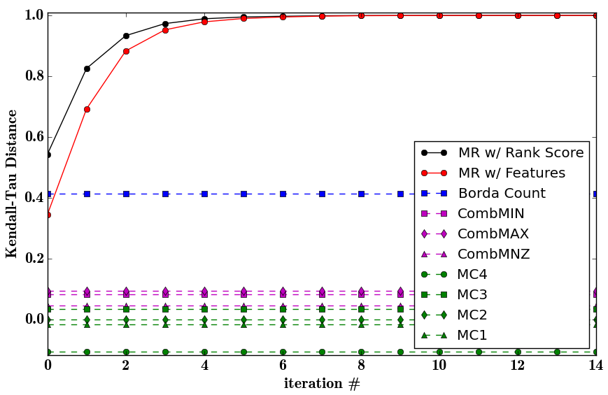
(a) subfig1

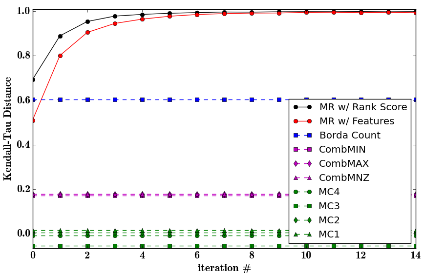
(b) subfig2

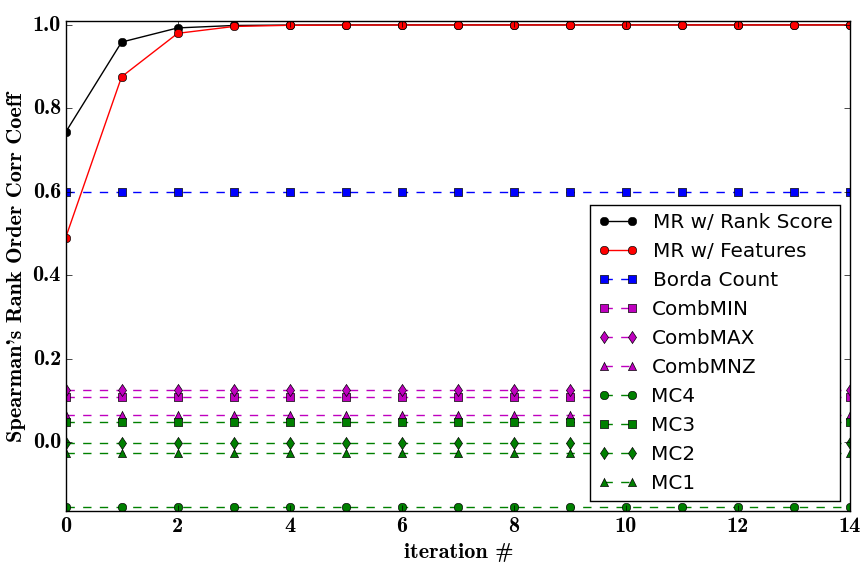
(c) subfig3

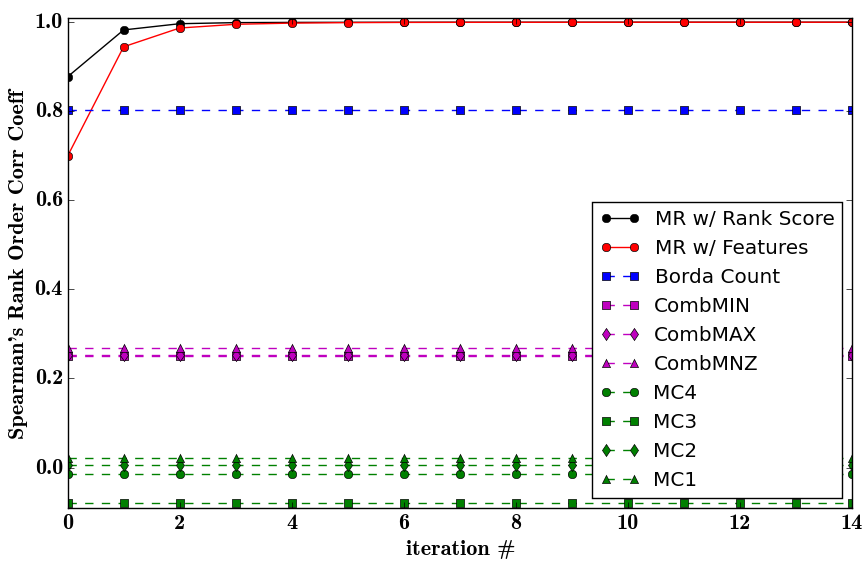
(d) subfig4

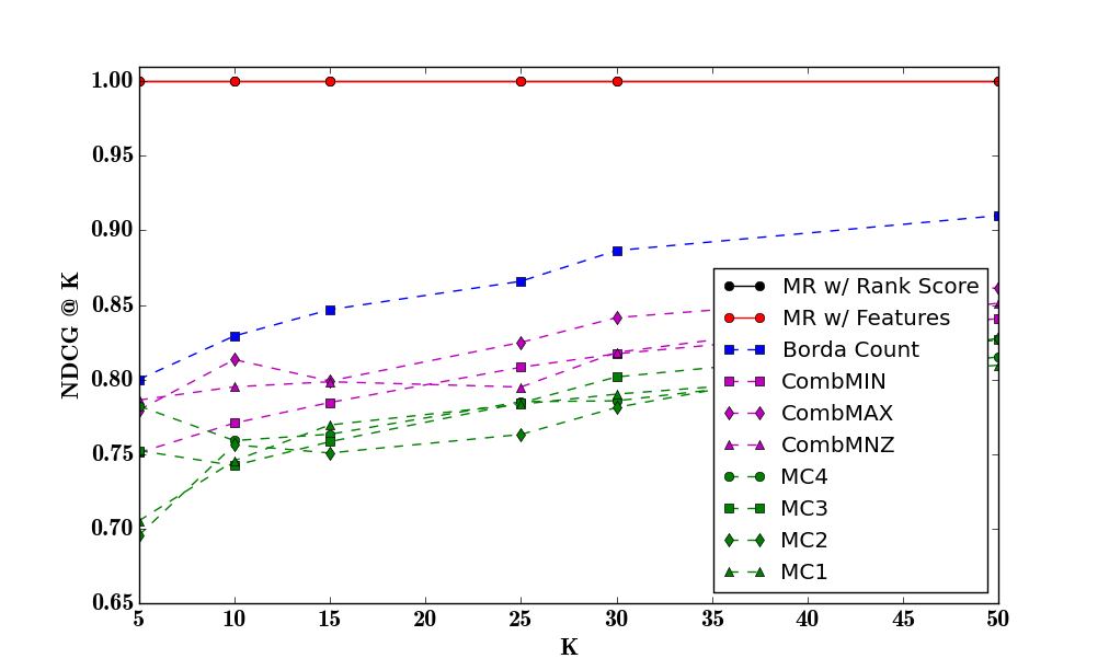
(e) subfig5

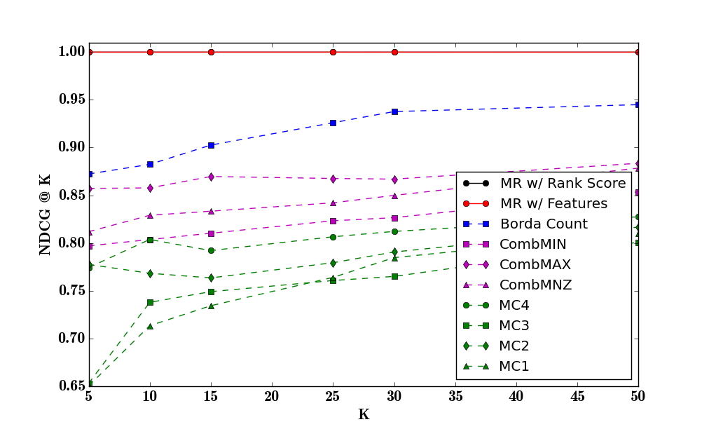
(f) subfig6

Figure 1: Synthetic Data: Kendall-Tau, Spearman’s Rho and NDCG@K vs K against iterations of the algorithm for Gaussian [figures ((1a)), ((1c)), ((1e)) respectively] and Poisson models [figures ((1a)), ((1d)), ((1f)) respectively]
Results show that our method can exactly recover the true rank order even from corrupted rank lists within only a few iterations. In contrast none of the baseline rank aggregation methods can recover the true ordering.

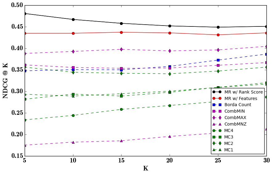
(a) subfig1

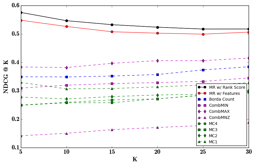
(b) subfig2

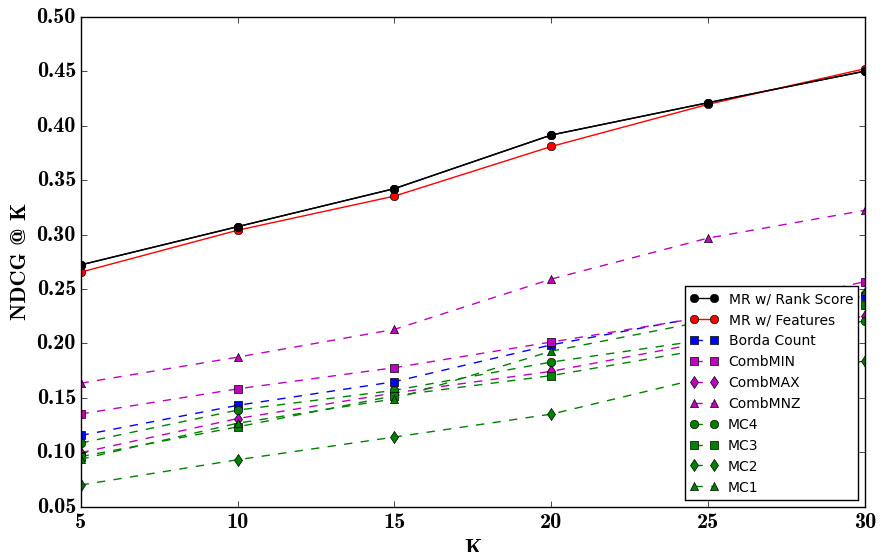
(c) subfig3

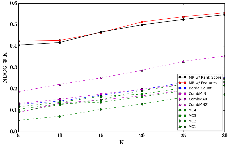
(d) subfig4

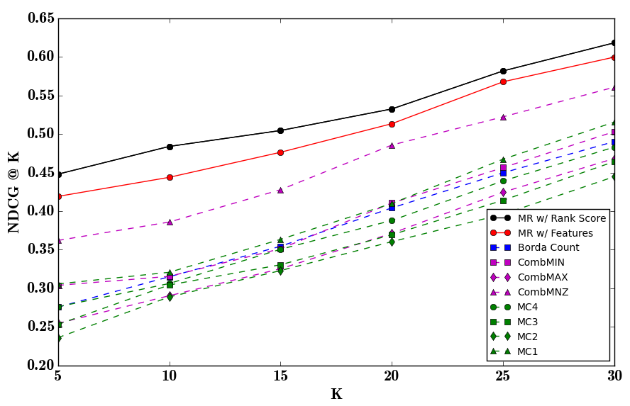
(e) subfig5

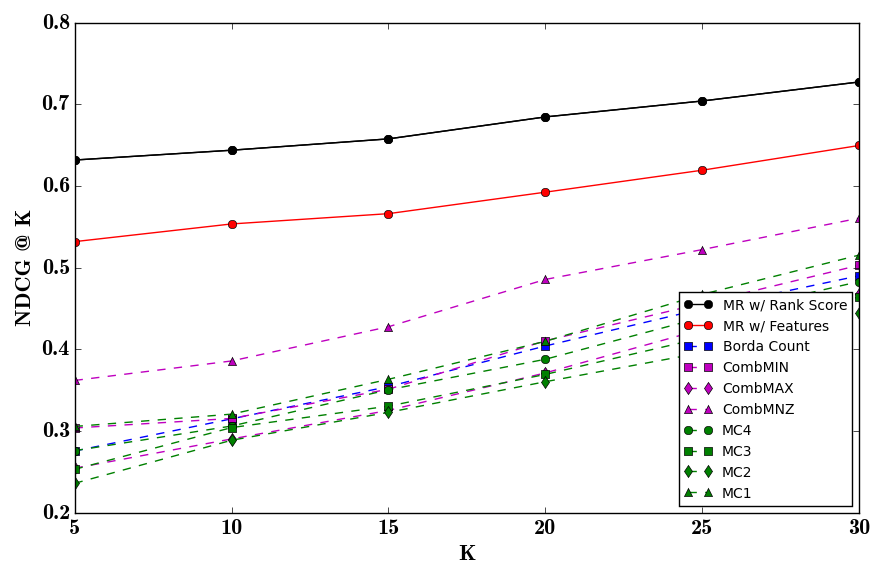
(f) subfig6

Figure 2: Real Datasets: NDCG@K versus K (higher is better) averaged across queries OHSUMED, MQ2008, MQ2007 datasets [figures: ((2a)), ((2c)), ((2e)) respectively], and NDCG@K vs K averaged across queries on the same datasets OHSUMED, MQ2008, MQ2007 with augmented rank lists [figures: ((2b)), ((2d)), ((2f)) respectively]
Results show that our methods outperform standard rank aggregation techniques in general. If the rank lists have ”good quality” experts, the improvement in performance is substantial for our method as opposed to baselines

6 Experiments

We evaluate the performance of our algorithm on both synthetic and real datasets. The metrics used for evaluation are Kendall’s tau coefficient [19] and Spearman’s rho or rank correlation coefficient [20], as well as the popular NDCG metric [17] for list-wise ranking. In all three metrics, a higher value indicates better recovery of rank order, and a value of 1.0 indicates exact order recovery.

As baselines, we use the classical Borda Count. Among linear combination methods, following [26] and [5] we use CombMNZ, and also show comparisons to non-linear aggregation methods like CombMIN and CombMAX [12]. Further, we also compare against all four Markov Chain based methods presented in [11].

6.1 Synthetic Data

We first evaluate on synthetic data where the GLM assumption holds (modulo noise). The rank aggregation framework is evaluated over $n=200$ items for each query. Matrix of feature vectors $\mathbf{X}$ is generated using the standard multivariate normal distribution and a normally distributed ${\bm{\omega}}^{*}$ is used to compute the true rank scores ${\bm{\rho}}^{*}$ from $\mathbf{X}{\bm{\omega}}^{*}$, according to the generalised linear models corresponding to Gaussian and Poisson distributions respectively, with the appropriate ${\bm{\phi}}$ function (see Appendix (A)).

The rank lists consist of vectors generated by randomly corrupting the true rank score ${\bm{\rho}}^{*}$ with different perturbations including translation, and additive or multiplicative noise. Multiple spurious expert rank lists are also generated as vectors constructed from pure random noise. In all, 10 rank lists are concatenated to form $\mathbf{R}$.

$\mathbf{X}$ and $\mathbf{R}$ are then used as input to our Algorithm (2) with the appropriate Bregman divergence and ${\bm{\phi}}(\cdot)$, and the outputs $\overline{\mathbf{z}}$ and $\overline{\mathbf{r}}$ are then evaluated against ${\bm{\rho}}^{*}$.

Figures ((1a)) and ((1c)) respectively show the value of Kendall’s tau and Spearman’s rho between the estimated $\overline{\mathbf{r}},\overline{\mathbf{z}}$ and the true ${\bm{\rho}}^{*}$ at each iteration of the algorithm, for the setup that uses a Gaussian model. Figures ((1b)) and ((1d)) show the same for a setup generated using a Poisson model. The plots show that in both models, the algorithm is able to exactly recover the original rank ordering (Kendall-tau and Spearman’s rho both evaluate to 1.0) within a small number of iterations. In contrast, none of the standard rank aggregation methods are able to recover the true ordering.

Figures ((1e)) and ((1f)) show NDCG@K vs K for the final ordering output by our method, as compared to baseline methods, in a Gaussian setup and a Poisson setup respectively. As opposed to the rank orderings output by our method which always perfectly extracts the top K items for each K, none of the baselines are able to correctly identify the top K relevant items for any value of K.

6.2 Real Datasets: MQ2008, MQ2007,
and OHSUMED

We evaluate our techniques as applied to the more challenging case of real datasets where the GLM assumption may not always hold. We use three complex real world datasets widely used for ranking applications- MQ2008 and MQ2007 from Microsoft’s LETOR 4.0 repository [31], and OHSUMED from the LETOR 3.0 repository [32].

The MQ2008 and the MQ 2007 datasets from the LETOR 4.0 repository are query sets from the Million Query track of TREC 2008. The LETOR 4.0 repository contains, for each query and associated document set, 46 object features for ranking as well as a set of 25 rank lists. We use the rank lists as our $\mathbf{R}$ and object features as our $\mathbf{X}$ matrix respectively. PageRank and relevance scores computed from different IR methods [18, 39] are also added to the rank lists (they are not used as object features).

The OHSUMED dataset is a subset of the MEDLINE database of medical publications, and the standard application involves extraction of relevant documents given a set of medical queries. The rank list matrix is constructed from 15 columns of the dataset that contain relevance scores computed using the BM25 score[18] and different IR methods based on language models [39]. The remaining 30 columns are used as object features.

In each of these datasets, we compare against ground truth which is available for each query and associated item as a relevance score that goes from 0 (not relevant) to 2 (most relevant) (ground truth is not used for learning). Additional details about the datasets including feature lists are available in [31] and [32] respectively. Note that for each experiment, object attributes and rank lists use disjoint sets of columns.

We compare the performance of different methods using the NDCG@K metric applied to this relevance score, averaged across queries for each K. The results are shown in figures ((2a)), ((2c)), ((2e)) for OHSUMED, MQ2008, MQ2007 respectively. The plots show that for all three datasets, even though the GLM assumption may not necessarily hold, our method nevertheless outperforms standard rank aggregation methods which do not take into account object features.

An interesting phenomenon that was observed with real datasets was that when at least one of the rank lists are of “high quality” in the sense that it is learned with supervision in the form of true relevance scores, the performance of our algorithm improves substantially. This effect is not seen on the baselines which only show marginal improvement compared to their performance on set of rank lists which has not been augmented with high quality lists.

We performed a similar experiments as above, except we augmented our rank lists from experts with the relevance scores output by a ranking function learned from training data using the methods in [3]. The NDCG@K versus K plots for augmented rank lists are shown for the OHSUMED dataset in fig. ((2b)), for the MQ2008 dataset in fig. ((2d)), and for the MQ2007 dataset in fig. ((2f)).

Side by side comparison with original plots show that when the rank lists contain at least one list of high quality, our algorithm returns an aggregated ordering in which the NDCG score shows a marked improvement, while standard methods fail to exploit the augmented rank lists to any substantial degree. Note that information about which rank lists are of high quality is not available to any of the algorithms in these experiments.

These experimental results suggest that if the set of rank lists are generated by sources whose expertise levels lie on a wide spectrum, our framework is nevertheless able to use more information from rank lists with higher credibility, and recover an ordering which matches the “true” ranking to a greater degree as compared to rank aggregation methods which depend solely on the rank lists and are blind to object features.

7 Conclusion

In this manuscript we introduced a novel rank aggregation scheme that augments expert rank lists with information from object features to bypass the various issues that plague the standard rank aggregation setup, and in the process obtain more accurate and robust aggregated rank scores. Experiments on synthetic data and on real datasets indicate that using object features can result in significant improvement in performance, more so when the rank lists contain orderings generated by sources with genuine expertise. Future work would cover theoretical analyses of our scheme, including statistical guarantees and extensions to more general models for ranking and rank aggregation.

APPENDIX

Appendix A Bregman Divergences

The matching loss functions associated with learning GLM parameters are distance-like functions called Bregman divergences, which are generalisations of square loss. Let ${\bm{\phi}}:\Theta\mapsto\mathbb{R}$ be a strictly convex, closed function on a convex domain $\Theta\subseteq\mathbb{R}^{m}$. Suppose ${\bm{\phi}}$ is differentiable on int($\Theta$). Then, for any $\mathbf{x},\mathbf{y}\in\Theta$, the Bregman divergence $D_{\bm{\phi}}(\cdot\|\cdot)$ between $\mathbf{y}$ and $\mathbf{x}$ corresponding to the function ${\bm{\phi}}$ is defined as

$$D_{\bm{\phi}}(\mathbf{y}\|\mathbf{x})\triangleq{\bm{\phi}}(\mathbf{y})-{\bm{\phi}}(\mathbf{x})-\langle\nabla{\bm{\phi}}(\mathbf{x}),\mathbf{y-x}\rangle$$

Bregman divergences are convex in their first argument. Although strictly speaking they are not a distance metric, they satisfy many properties of metrics, for example $D_{\bm{\phi}}(\mathbf{y}\|\mathbf{x})\geq 0$ and $D_{\bm{\phi}}(\mathbf{y}\|\mathbf{x})=0$ if and only if $\mathbf{y=x}$. Many standard distance-like functions like Square loss and KL-divergence are members of this family (see Table (1)).

There is a one-one correspondence between each GLM and each Bregman divergence via the convex function ${\bm{\phi}}(\cdot)$, and parameter estimation in a GLM with given object features $\mathbf{X}$ and target variable $\overline{\mathbf{z}}$ is equivalent to finding the minimiser for $D_{\bm{\phi}}\left(\mathbf{z}\|(\nabla{\phi})^{-1}(\mathbf{X{\bm{\omega}}})\right)$ over ${\bm{\omega}}$, where ${\bm{\phi}}(\cdot)$ is the convex function associated with the particular GLM used (refer to [6] for a detailed exposition on the relationship between Bregman Divergences and GLM’s).

${\bm{\phi}}(\mathbf{x}$)	$D_{\bm{\phi}}(\mathbf{y\|x})$
$\frac{1}{2}\|\mathbf{x}\|^{2}$	$\frac{1}{2}\|\mathbf{y-x}\|^{2}$
$\sum_{i}(x^{(i)}\log x^{(i)})$ $\mathbf{x}\in$ Prob. Simplex	KL($\mathbf{y\|x}$) = $\sum_{i}\left(y^{(i)}\log(\frac{y^{(i)}}{x^{(i)}})\right)$
$\sum_{i}\left(x^{(i)}\log x^{(i)}-x^{(i)}\right)$ $\mathbf{x}\in\mathbb{R}^{n}_{+}$	GI($\mathbf{y\|x}$) = $\sum_{i}y^{(i)}\log(\frac{y^{(i)}}{x^{(i)}})-y^{(i)}+x^{(i)}$

Table 1: Examples of Bregman Divergences

Appendix B Monotone Retargeting

Monotone retargeting [3, 1] or MR is a LETOR framework that models ranking functions of object features on monotonic transformations of given relevance scores, and learns both the ranking function as well as the best monotonic transformation. The paper [3] solves the LETOR problem using MR by modeling the monotonically transformed rank score $\overline{\mathbf{z}}$ as a generalised linear model over object features $\mathbf{X}$ and learns the GLM parameter ${\bm{\omega}}$ that best fits the data over all possible monotonic transformations $\overline{\mathbf{z}}$ of the given “true” relevance scores ${\bm{\rho}}^{*}$.

The LETOR setup used by MR is the following. Consider a single query. Suppose for a given set of $n$ items $\{V_{1},V_{2},\cdots V_{n}\}$ to be ranked, $\mathbf{X}\in\mathbb{R}^{n\times p}$ is the matrix of object features. Suppose the supervision is provided as a rank score vector ${\bm{\rho}}^{*}\in\mathbb{R}^{n}$. The objective of MR is to find a monotonic transformation of the given rank scores $\overline{\mathbf{z}}\sim_{\downarrow}{\bm{\rho}}^{*}$ and a real valued parameter ${\bm{\omega}}\in\mathbb{R}^{p}$ which minimises the Bregman divergence $D_{{\bm{\phi}}}\left({\overline{\mathbf{z}}}\|(\nabla{\phi})^{-1}({\mathbf{X}{\bm{\omega}}})\right)$. The optimisation problem, therefore, is the following

$$\underset{\overline{\mathbf{z}},{\bm{\omega}}}{\text{min}} D_{\bm{\phi}}\left(\mathbf{z}\|(\nabla{\phi})^{-1}(\mathbf{X{\bm{\omega}}})\right)$$ (8)

s.t. $$\overline{\mathbf{z}}\sim_{\downarrow}{\bm{\rho}}^{*}$$

Given ${\bm{\rho}}^{*}$ and $\mathbf{X}$, this problem is separately convex in $\overline{\mathbf{z}}$ and ${\bm{\omega}}$, and with appropriate regularisation can also be made jointly convex in the two variables[1]. A top level description of the algorithm as adapted from [3] is presented as Algorithm (1) in the main manuscript. In particular, the steps involved include a standard GLM parameter estimation for ${\bm{\omega}}$ and the pool adjacent violators algorithm [13], widely used in isotonic regression, for $\overline{\mathbf{z}}$. If ${\bm{\rho}}^{*}$ is partially ordered, an intermediate step involves the estimation of a total ordering consistent with the partial ordering specified by ${\bm{\rho}}^{*}$. Each step of the algorithm has been widely studied in the literature and off-the-shelf solvers can be used to efficiently iterate through each step of the algorithm to converge to a stationary point. See [3] for a more detailed discussion on the properties of the solution obtained via this framework, and efficient algorithms for optimisation.

Appendix C Margin Equipped Monotone Retargeting

A margin equipped variation of this problem, MEMR[1], avoids degenerate stationary points by enforcing a margin between the relevance score between any two items in the setup. That is, suppose ${\bm{\epsilon}}=[\epsilon_{1},\epsilon_{2},\cdots\epsilon_{n-1}]\in\mathbb{R}^{n-1}_{+}$, where each $\epsilon_{j}\geq 0$. Suppose the specified rank score vector ${\bm{\rho}}^{*}$ is ordered as $(\tau_{1},\tau_{2},\cdots\tau_{n})$, where each $\tau_{j}\in\{1,2,\cdots,n\}$. That is, ${\bm{\rho}}^{\tau_{j}}\geq{\bm{\rho}}^{\tau_{j+1}}$ for each $j=1,2,\cdots(n-1)$. Then the reformulated optimisation problem used in MEMR is as follows

$$\underset{\overline{\mathbf{z}},{\bm{\beta}}}{\text{min}} D_{\bm{\phi}}\left(\mathbf{z}\|(\nabla{\phi})^{-1}(\mathbf{X{\bm{\beta}}})\right)$$ (9)

s.t. $$\overline{\mathbf{z}}\sim_{\downarrow}{\bm{\rho}}^{*}$$

$$\overline{\mathbf{z}}^{\tau_{j}}-\overline{\mathbf{z}}^{\tau_{j+1}}\geq\epsilon_{j}\ \ \forall\ j=1,2,\cdots n-1$$

Since the additional constraints are convex half-space constraints over $\overline{\mathbf{z}}$, most of the standard properties of monotone retargeting are maintained (see [1] for a more detailed analysis as well as optimisation algorithms).

References

- [1] S. Acharyya and J. Ghosh. MEMR: A margin equipped monotone retargeting framework for ranking. In Proceedings of the Thirtieth Conference on Uncertainty in Artificial Intelligence, 2014.
- [2] S. Acharyya and J. Ghosh. Parameter estimation of generalized linear models without assuming their link function. Proceedings of the Eighteenth International Conference on Artificial Intelligence and Statistics, 2015.
- [3] S. Acharyya, O. Koyejo, and J. Ghosh. Learning to Rank with Bregman Divergences and Monotone Retargeting . In Proc. UAI 2012, pages 15–25, 2012.
- [4] K. J. Arrow. A difficulty in the concept of social welfare. The Journal of Political Economy, pages 328–346, 1950.
- [5] J. A. Aslam and M. Montague. Models for metasearch. In Proceedings of the 24th annual international ACM SIGIR conference on Research and development in information retrieval, pages 276–284. ACM, 2001.
- [6] A. Banerjee, S. Merugu, I. S. Dhillon, and J. Ghosh. Clustering with Bregman divergences. The Journal of Machine Learning Research, 6:1705–1749, 2005.
- [7] A. Bhowmik, J. Ghosh, and O. Koyejo. Generalized Linear Models for Aggregated Data. In Proceedings of the Eighteenth International Conference on Artificial Intelligence and Statistics, pages 93–101, 2015.
- [8] D. Black. On the rationale of group decision-making. The Journal of Political Economy, pages 23–34, 1948.
- [9] C. Cavanagh and R. P. Sherman. Rank estimators for monotonic index models. Journal of Econometrics, 84(2):351–381, 1998.
- [10] S. Chen, F. Wang, Y. Song, and C. Zhang. Semi-supervised ranking aggregation. Information Processing & Management, 47(3):415–425, 2011.
- [11] C. Dwork, R. Kumar, M. Naor, and D. Sivakumar. Rank aggregation revisited, 2001.
- [12] J. A. Fox and E. Shaw. Combination of multiple sources: The trec-2 interactive track matrix experiment. In ACM SIGIR-94, 1994.
- [13] S. Grotzinger and C. Witzgall. Projections onto order simplexes. Applied mathematics and Optimization, 12(1):247–270, 1984.
- [14] R. Herbrich, T. Graepel, and K. Obermayer. Support vector learning for ordinal regression. 1999.
- [15] S. C. Hoi and R. Jin. Semi-supervised ensemble ranking. In AAAI, pages 634–639, 2008.
- [16] R. Iyer and J. Bilmes. The lovász-bregman divergence and connections to rank aggregation, clustering, and web ranking. Uncertainity in Artificial Intelligence, 2013.
- [17] K. Järvelin and J. Kekäläinen. Ir evaluation methods for retrieving highly relevant documents. In Proceedings of the 23rd annual international ACM SIGIR conference on Research and development in information retrieval, pages 41–48. ACM, 2000.
- [18] K. S. Jones, S. Walker, and S. E. Robertson. A probabilistic model of information retrieval: development and comparative experiments: Part 2. Information Processing & Management, 36(6):809–840, 2000.
- [19] M. G. Kendall. A new measure of rank correlation. Biometrika, pages 81–93, 1938.
- [20] M. G. Kendall. Rank correlation methods. 1948.
- [21] A. Klementiev, D. Roth, and K. Small. Unsupervised rank aggregation with distance-based models. In Proceedings of the 25th international conference on Machine learning, pages 472–479. ACM, 2008.
- [22] A. Klementiev, D. Roth, and K. Small. Unsupervised rank aggregation with distance-based models. In Proceedings of the 25th international conference on Machine learning, pages 472–479. ACM, 2008.
- [23] A. Klementiev, D. Roth, K. Small, and I. Titov. Unsupervised rank aggregation with domain-specific expertise. Urbana, 51:61801, 2009.
- [24] O. Koyejo, S. Acharyya, and J. Ghosh. Retargeted matrix factorization for collaborative filtering. In Proceedings of the 7th ACM conference on Recommender systems, pages 49–56. ACM, 2013.
- [25] G. Lebanon and J. Lafferty. Cranking: Combining rankings using conditional probability models on permutations. In ICML, volume 2, pages 363–370, 2002.
- [26] J. H. Lee. Analyses of multiple evidence combination. In ACM SIGIR Forum, volume 31, pages 267–276. ACM, 1997.
- [27] H. Li. Learning to rank for information retrieval and natural language processing. Synthesis Lectures on Human Language Technologies, 7(3):1–121, 2014.
- [28] Y.-T. Liu, T.-Y. Liu, T. Qin, Z.-M. Ma, and H. Li. Supervised rank aggregation. In Proceedings of the 16th international conference on World Wide Web, pages 481–490. ACM, 2007.
- [29] P. McCullagh and J. A. Nelder. Generalized linear models. 1989.
- [30] M. Pujari and R. Kanawati. Supervised rank aggregation approach for link prediction in complex networks. In Proceedings of the 21st international conference companion on world wide web, pages 1189–1196. ACM, 2012.
- [31] T. Qin and T.-Y. Liu. Introducing letor 4.0 datasets. arXiv preprint arXiv:1306.2597, 2013.
- [32] T. Qin, T.-Y. Liu, J. Xu, and H. Li. Letor: A benchmark collection for research on learning to rank for information retrieval. Information Retrieval, 13(4):346–374, 2010.
- [33] V. Raman and S. Saurabh. Parameterized algorithms for feedback set problems and their duals in tournaments. Theoretical Computer Science, 351(3):446–458, 2006.
- [34] S. Rendle, C. Freudenthaler, Z. Gantner, and L. Schmidt-Thieme. BPR: Bayesian personalized ranking from implicit feedback. In Proceedings of the Twenty-Fifth Conference on Uncertainty in Artificial Intelligence, pages 452–461. AUAI Press, 2009.
- [35] D. G. Saari. Explaining all three-alternative voting outcomes. Journal of Economic Theory, 87(2):313–355, 1999.
- [36] Q. F. Stout. Fastest isotonic regression algorithms, 2014.
- [37] K. Subbian and P. Melville. Supervised rank aggregation for predicting influencers in twitter. In Privacy, Security, Risk and Trust (PASSAT) and 2011 IEEE Third Inernational Conference on Social Computing (SocialCom), 2011 IEEE Third International Conference on, pages 661–665. IEEE, 2011.
- [38] M. Van Erp and L. Schomaker. Variants of the borda count method for combining ranked classifier hypotheses. In Seventh International Workshop on Frontiers in Handwriting Recognition, 2000.
- [39] C. Zhai and J. Lafferty. A study of smoothing methods for language models applied to ad hoc information retrieval. In Proceedings of the 24th annual international ACM SIGIR conference on Research and development in information retrieval, pages 334–342. ACM, 2001.