Discovery of an extremely weak magnetic field in the white dwarf LTT 16093 = WD 2047+372

Abstract

Context. Magnetic fields have been detected in several hundred white dwarfs, with strengths ranging from a few kG to several hundred MG. Only a few of the known fields have a mean magnetic field modulus below about 1 MG.

Aims. We are searching for new examples of magnetic white dwarfs with very weak fields, and trying to model the few known examples. Our search is intended to be sensitive enough to detect fields at the few kG level.

Methods. We have been surveying bright white dwarfs for very weak fields using spectropolarimeters at the Canada-France-Hawaii telescope, the William Herschel telescope, the European Southern Observatory, and the Russian Special Astrophysical Observatory. We discuss in some detail tests of the WHT spectropolarimeter ISIS using the known magnetic strong-field Ap star HD 215441 (Babcock’s star) and the long-period Ap star HD 201601 ($\gamma$ Equ).

Results. We report the discovery of a field with a mean field modulus of about 57 kG in the white dwarf LTT 16093 = WD 2047+372. The field is clearly detected through the Zeeman splitting of H$\alpha$ seen in two separate circularly polarised spectra from two different spectropolarimeters. Zeeman circular polarisation is also detected, but only barely above the $3\sigma$ level.

Conclusions. The discovery of this field is significant because it is the third weakest field ever unambiguously discovered in a white dwarf, while still being large enough that we should be able to model the field structure in some detail with future observations.

1 Introduction

Magnetic fields in stars are increasingly recognised as a source of significant physical effects (such as transfer of angular momentum and influence on accretion and mass loss), and as a phenomenon affecting other physical processes (such as convection and internal shear). On the basis of many recent observations, we now know something about the occurrence of magnetic fields in most of the main stages of stellar evolution, from the pre-main sequence (Donati & Landstreet 2009; Hussain 2012; Alecian et al. 2013) through the main sequence (Donati & Landstreet 2009; Petit et al. 2013; Wade & MiMeS Collaboration 2015), the red giant (Aurière et al. 2015) and asymptotic giant (Grunhut et al. 2010) stages, and finally the white dwarf stage (Kepler et al. 2013; Ferrario et al. 2015).

In general, the magnetic fields of non-degenerate stars with low effective temperatures ($T_{\mathrm{eff}}\ \la 6500-7000$ K) have fields driven by current dynamo action, analogous to the situation in the Sun. Fields are generally stronger in relatively rapid rotating stars than in more slowly rotating stars, and the fields often have complex surface structure which changes on a rather short timescale.

Magnetic fields are found only in a few percent of stars hotter than $\sim 7000$ K, and they do not seem to be powered by stellar rotation. In fact, the strongest fields are found on stars that are unusually slowly rotating stars. The fields of hotter stars have a considerably simpler structure than those of cooler stars, usually of qualitatively dipolar topology, and their structure does not change significantly on timescales of decades. The magnetic fields of white dwarfs are generally of this second (“fossil”) variety.

Although we now have observational information about what kinds of fields occur in various stages of evolution, the physics underlying the transformations of field strength and structure during long evolutionary stages (such as the main sequence or the white dwarf state) or between successive stages (such as from the red giant to the white dwarf state) are far from clear. A particularly challenging aspect of this general question is to understand the processes that occur as a stellar field evolves from fossil to dynamo or vice versa. An important goal of current magnetic studies is to try to shed light on this evolution. As a particular example, the fossil fields found in a few percent of white dwarfs are thought to originate in an earlier evolution stage of the star, and thus these fields potentially carry useful information about the processes that occur as a magnetic white dwarf forms from the preceding giant stage, or perhaps as it forms as a result of a merger process in a close binary system sometime during that giant stages (Valyavin & Fabrika 1999; Tout et al. 2008; Wickramasinghe et al. 2014).

Observationally, the kinds of information that may potentially illuminate how magnetic fields developed and evolved after the red giant stage are (1) the surface structures of the magnetic fields of a suitable sample of white dwarfs, and (2) the frequency and distribution of field strengths found in white dwarfs as functions of age, mass, and surface composition.

At present, several hundred magnetic white dwarfs have been identified, mostly by observation of magnetic (Zeeman) splitting of spectral lines. Many of the known magnetic white dwarfs have been found recently from the Sloan Digital Sky Survey (SDSS, Kepler et al. 2013). This survey (and most other surveys for white dwarfs) have been carried out using low resolution (and frequently low S/N) spectroscopy. With such data it is not possible to recognise magnetic splitting in white dwarfs with fields less than about 1 MG. However, it is known that white dwarf magnetic fields as weak as a few kG occur (e.g., Aznar Cuadrado et al. 2004). The total range of field strengths is thus more than four dex, from below 20 kG to about 800 MG (Ferrario et al. 2015).

In contrast to the high-field regime of the white dwarf field strength distribution, very little is known about the weak-field limit. If we measure the typical strength of the field by the mean field modulus $\langle|B|\rangle$, an average of the scalar field over the visible hemisphere of the star, only about a dozen white dwarfs are known to have magnetic fields with $\langle|B|\rangle\ \la 300$ kG. Consequently the field strength distribution over mass, age, and composition in the weak-field limit is very poorly constrained. The weakest fields now known are certainly right at the detectability threshold. It is therefore not known whether the detected weak-field white dwarfs are near the lower limit of the complete field strength distribution, or whether this distribution continues to still weaker fields that are currently undetectable. The single piece of data that we have on the regime below 1 kG is the observation that $|\langle B_{z}\rangle|\la 250$ G ($3\sigma$ limit) in the bright DA white dwarf 40 Eri B (Landstreet et al. 2015).

Apart from the uncertainty of their actual incidence, the morphologies of the known weak-fields in WDs have never been modelled in detail – only a couple of stars have even been modelled with the simplest structures that might be appropriate, for example a magnetic dipole centred on the star but possibly inclined to the rotation axis (Valyavin et al. 2005, 2008; Landstreet et al. 2012).

We have been carrying out a search for extremely weak fields among bright ($V\leq 13.5$) white dwarfs, using spectropolarimetry and high resolution spectroscopy, both of which are sensitive to kG fields, far below the 1 MG detection threshhold of low resolution spectroscopy. In the course of this survey, we have discovered an extremely weak magnetic field in the DA3.4 white dwarf LTT 16093 = WD 2047+372. The field of this star has $\langle|B|\rangle\approx 57$ kG. Only two magnetic white dwarfs are known that are definitely magnetic but have fields for which $\langle|B|\rangle$ falls below this value. Thus this star is an important addition to a very small sample. In this paper we report the details of this discovery, and describe what we can deduce about the star from the data obtained so far.

2 Observations

As discussed in detail by Koester et al. (1998, 2009); Landstreet et al. (2015), searches for weak fields in white dwarfs using unpolarised spectroscopy can detect fields as low as $\langle|B|\rangle\sim 10-20$ kG provided the spectrograph has resolving power of $R\ga 20\,000$. Still weaker fields can be detected with spectropolarimetry, measuring $\langle B_{z}\rangle$, the line-of-sight component of the magnetic field averaged over the visible stellar hemisphere. $\langle B_{z}\rangle$ may be measured either using a low or mid resolution spectropolarimeter such as FORS at the European Southern Observatory ($R$ up to $\sim 2000$), ISIS on the William Herschel Telescope ($R$ up to $\sim 8000$), or the Main Stellar Spectrograph of the Special Astrophysical Observatory of the Russian Academy of Sciences ($R$ up to 6000), that can measure the small circular polarisation in the broad wings of H or He lines (Bagnulo et al. 2002; Aznar Cuadrado et al. 2004), or using a high resolution spectropolarimeter such as ESPaDOnS at the Canada-France-Hawaii Telescope to measure the circular polarisation signal in the core of the Balmer H$\alpha$ line (Landstreet et al. 2015). We have used all of these spectropolarimeters in our searches for weak fields.

2.1 Observations of WD 2047+372 with ESPaDOnS

ESPaDOnS is a high resolution cross-dispersed echelle spectropolarimeter, constructed for the Canada-France-Hawaii Telescope. The instrument produces an almost complete spectrum between about 3800 and 10 400 Å, with a typical resolving power of about 65 000. ESPaDOnS can measure the intensity spectrum $I$, together with one of the other three Stokes components $Q$, $U$ (linear polarisation) or $V$ (circular polarisation) as functions of wavelength. (The $I$ spectrum, of course, is simply a measurement of the incoming stellar flux as a function of wavelength, as modified by the terrestrial atmosphere, by the telescope and instrument transmission functions, and by the efficiency of the detector.)

The instrument consists of a polarisation analyser mounted at the Cassegrain focus of the 3.6-m telescope, and a bench mounted spectrograph. In the polarisation analyser, a series of Fresnel rhombs are combined in such a way as to act as a fully achromatic rotating $\lambda/4$ or $\lambda/2$ waveplate. The retarder is followed by a small-angle beam-splitting Wollaston prism, and the entrance aperture is re-imaged onto two fibre optic cable ends. The two beams which carry the intensities of the two orthogonal polarisation states are transferred by the fibre optic cables to a temperature-stabilised, bench-mounted cross-dispersed echelle spectrograph which splits the observed spectrum into 40 orders, ranging in wavelength extent per order from about 100 Å (near 4000 Å) to more than 300 Å (near 10 000 Å).

Because the entrances to the fibre optic cables follow the polarising optics, and act as stops, the relative intensity of the two beams may vary slightly with seeing and flexure between one exposure and the next, even if the stellar beam is completely unpolarised. As a result the broad-band polarisation of the incoming beam cannot be measured accurately with ESPaDOnS. Line polarisation may however be very accurately measured with respect to the nearby continuum, which is in fact set to zero by the ESPaDOnS pipeline. This situation is perfectly satisfactory when the continuum may be assumed to be unpolarised.

The broad wings of the Balmer lines of white dwarfs cover wavelength ranges comparable to the width of single orders of the echelle spectrograph, and measuring the polarisation in their broad wings presents almost the same problems as detecting polarisation in the continuum. Practically, the polarisation in the outer Balmer line wings of magnetic white dwarfs is largely undetectable by ESPaDOnS (and presumably by other similar high resolution spectropolarimeters), although (depending on the details of instrumental continuum polarisation removal) some polarisation may still be detectable in the inner Balmer line wings within a few Å of the line core. However, it is quite practical to measure the magnetic field from the analysis of the sharp core of H$\alpha$. Because this core is much narrower than the FWHM of the full Balmer line, the $V/I$ polarisation signal in the wings of the sharp core is much larger than that in the broad wings, and is not affected by the removal of broad-band instrumental polarisation. We have previously used high resolution spectropolarimetry of this feature to set a very low upper limit on a possible large-scale magnetic field in the bright white dwarf 40 Eri B (Landstreet et al. 2015). In that study we showed that the line core is indeed about as sensitive to non-zero $\langle B_{z}\rangle$ fields as we expected, by measuring fields with the very similar H$\alpha$ line cores found in several main sequence B stars. It is found that because the line core is narrow and deep, this single feature makes possible $\langle B_{z}\rangle$ field measurements that are competitive in terms of field strength uncertainties to more conventional measurements using full line wings. Compared to low resolution spectropolarimeters, a further major advantage of the use of ESPaDOnS is that its higher spectral resolution allows us to simultaneously detect more subtle Zeeman splitting in Stokes $I$. As a result, field measurements of white dwarfs using high resolution provide excellent sensitivity and accuracy for determination of the mean field modulus $\langle|B|\rangle$ of the magnetic field.

We acquired one ESPaDOnS circularly polarised spectrum of WD 2047+372, on 2015 October 31 at 06:20 UT, MJD 57326.255, requiring $4\times 814=3256$ s total shutter time. A small window around H$\alpha$ is shown in Figure 1. The H$\alpha$ spectra from two normalised overlapping orders have been combined by weighted averaging. Then both the intensity ($I$) and circularly polarised ($V/I$) spectra have been binned over wavelength intervals of 0.2 Å, which substantially improves the S/N ratio of each plotted point of the $I$ and $V/I$ Stokes components, without significantly degrading the resolution of the features in these spectra.

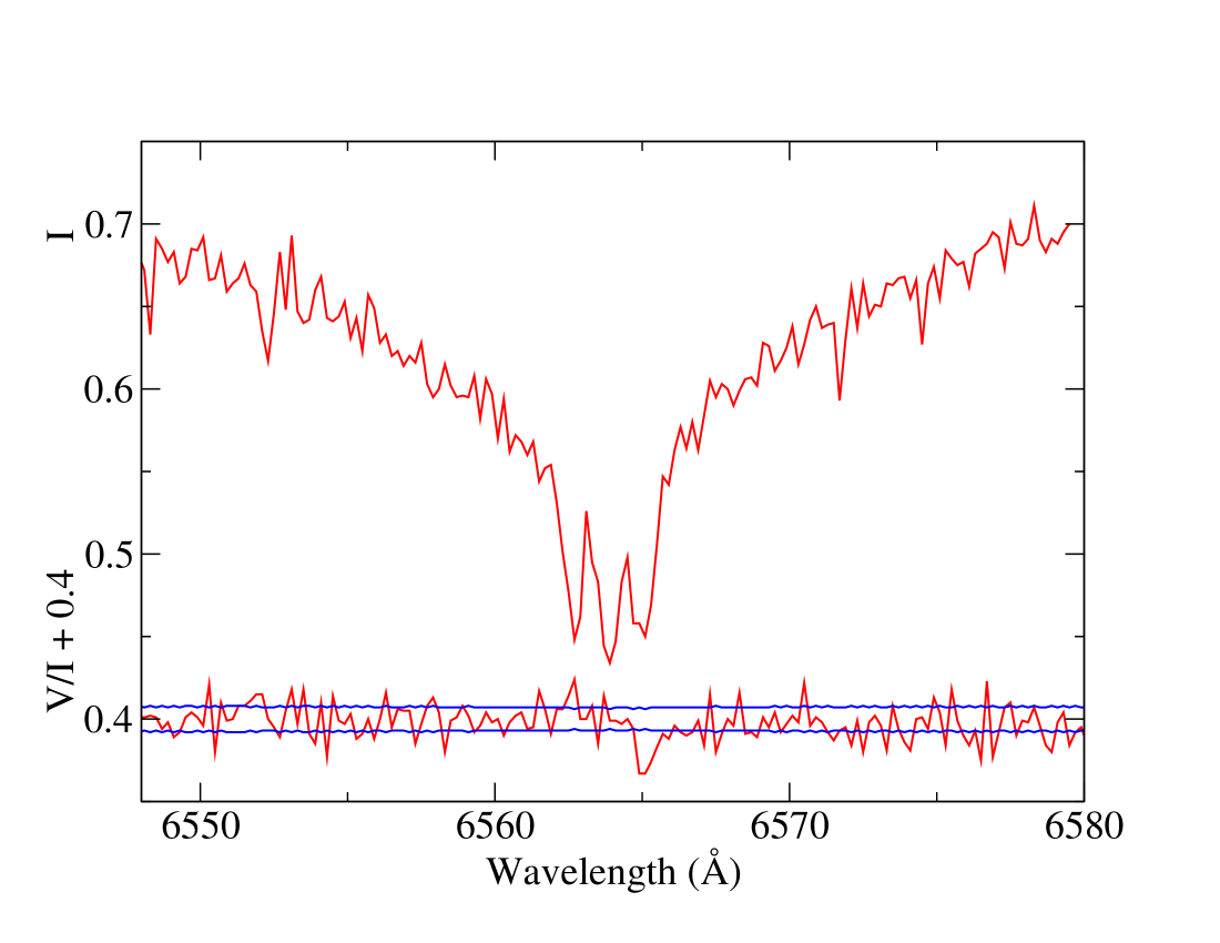
Figure 1: Deep $I$ H$\alpha$ line core (upper curve) and observed $V/I$ circular polarisation spectrum (lower curve) of WD 2047+372, binned over intervals of 0.2 Å and arbitrarily normalised. The $V/I$ spectrum is moved upwards by +0.4 vertical units to facilitate comparison with the $I$ spectrum. We also plot the $\pm 1\sigma$ level of photon noise bracketting the observed $V/I$ spectrum, both lines also shifted upwards by +0.4.

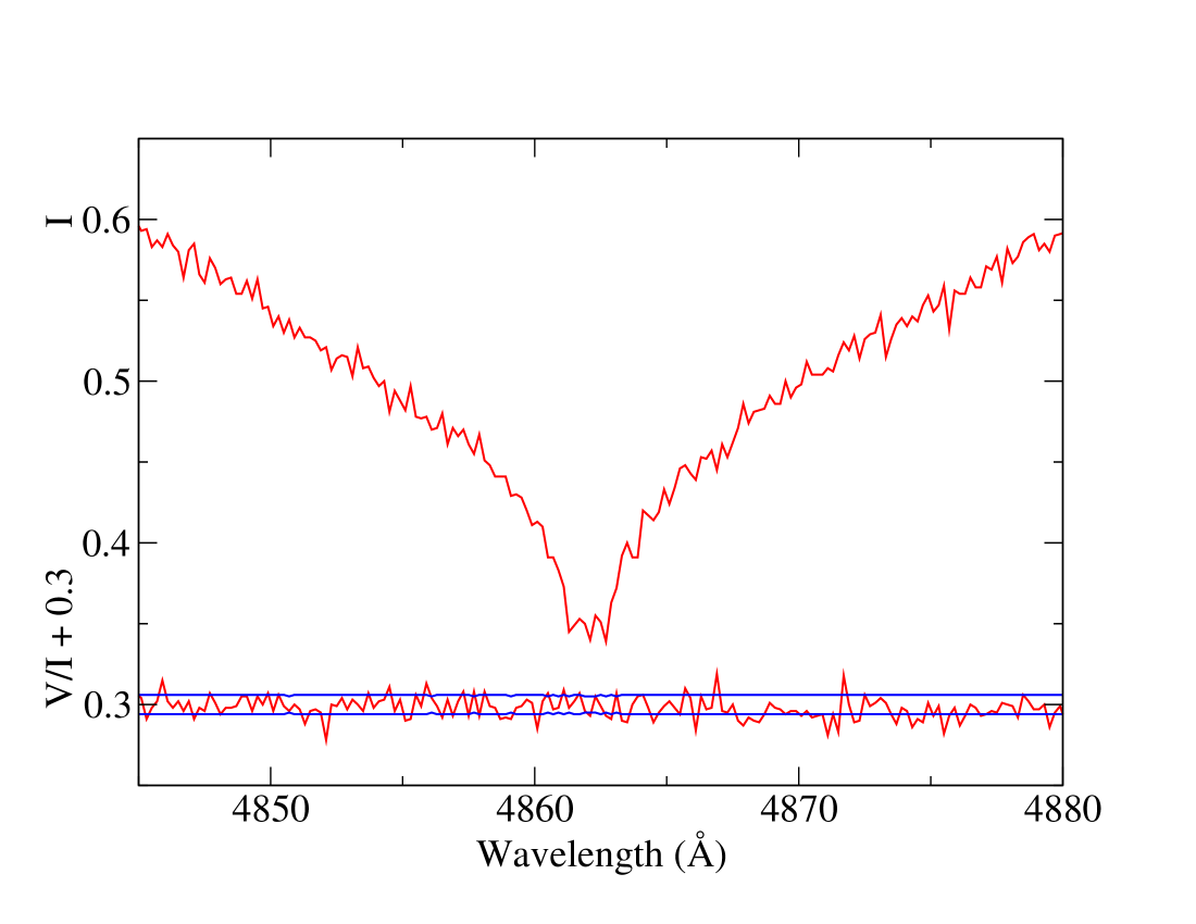
Figure 2: H$\beta$ line core of WD 2047+372. The meaning of symbols is as in Figure 1. The $V/I$ signal and its associated $\pm 1\sigma$ error bars have been shifted vertically by +0.3.

The very obvious magnetic signature in Fig. 1 is the clear splitting of the line core into a Zeeman triplet. Strikingly, the two flanking $\sigma$ components are no wider than the central $\pi$ component, suggesting that the dispersion in local field strength $|B(x,y)|$ is not a great deal larger than about 0.2 or 0.3 of its actual value. The wavelength position of each of the components of the Zeeman triplet was measured using the IRAF “splot” function to measure the barycentre of the component after subtracting the linear continuum marked by the user. The uncertainty of these measurements was estimated by repeating them. The results are that the separation of the blue $\sigma$ component from the $\pi$ component is about $1.152\pm 0.01$ Å, and that of the red component is about $1.139\pm 0.01$ Å, for an average of $1.145\pm 0.007$ Å. Using the simple expression for the separation of the $\sigma$ components from the wavelength of the line in zero field,

$$\Delta\lambda_{\rm Z}=C_{\rm z}g_{\rm eff}\lambda_{0}^{2}B,$$ (1)

where $C_{z}=4.67\,10^{-13}$ Å^-1 G^-1 is a constant, wavelengths are measured in Å and the field in G, the Landé factor of the H$\alpha$ line $g_{\rm eff}=1.0$ (Casini & Landi Degl’Innocenti 1994), and the mean measured separation corresponds to a mean magnetic field modulus, suitably averaged over the visible hemisphere, of $\langle|B|\rangle=56.9\pm 0.4$ kG. It is quite clear that WD 2047+372 hosts a magnetic field of a little less than 60 kG.

The core of the H$\beta$ line of WD 2047+372, shown in Figure 2, has an abnormal flat bottom, and if the weak structure in that core is interpreted as incipient Zeeman splitting, the estimated field is fully compatible in strength to that measured from the H$\alpha$ line core.

Although the circular polarisation seen in Figure 1 is non-zero only at a fairly marginal level, the circular polarisation $V/I$ shows weak peaks of opposite sign at the positions of the two $\sigma$ components. This weak signal in $V/I$ is consistent with a slightly non-zero value of $\langle B_{z}\rangle$. The field can be evaluated using the standard expression for measuring the separation between the mean wavelengths of the right and left circularly polarised line cores,

$$\langle B_{z}\rangle=-2.14\,10^{12}\frac{\int vV(v){\rm d}v}{g_{\rm eff}\lambda_{0}c\int(I_{\rm cont}-I(v)){\rm d}v}$$ (2)

where $I$ and $V$ are expresed as functions of velocity $v$ relative to line centre at $\lambda_{)}$, and $c$ is the speed of light (Mathys 1989; Donati et al. 1997). The Landé factor $g_{\rm eff}=1.0$ (Casini & Landi Degl’Innocenti 1994). The numerical evaluation of this expression and its uncertainty are discussed by Landstreet et al. (2015).

Evaluating the integrals over the full width and depth of the line core below the broad line, we find $\langle B_{z}\rangle=+6000\pm 1670$ G, barely significant at the $3.6\sigma$ level.

2.2 Observations of WD 2047+372 with ISIS at the WHT

The Intermediate dispersion Spectrograph and Imaging System (ISIS) is a medium resolution spectrograph, equipped with polarimetric optics, mounted at the Cassegrain focus of the 4.2 m William Herschel Telescope (WHT) on La Palma. The use of a dichroic filter permits simultaneous observing in two arms, one optimised for the blue and one for the red wavelength range. In our observations we used the grism 600B in the blue arm, with a dispersion of 0.45 Å per pixel and spectral resolving power of 2200 (1″slit width), and grism 1200R in the red arm, with a dispersion of 0.26 Å per pixel and a spectral resolving power of 7400 (1″ slit width). The grisms were mounted such as to cover the spectral ranges of $\sim 3700-5200$ Å and $\sim 6100-6850$ Å in the blue and in the red arm, respectively.

The polarimetric optics consist of an achromatic $\lambda/4$ retarder waveplate followed by a Savart plate. A decker with three $18\arcsec$ strips prevent the overlapping of the two beams split by the Savart plate, and allows sampling the sky background on two regions adjacent to the target. The instrument can measure both continuum and line polarisation. Its magnetographic capabilities are somewhat limited by the fact that its spectral resolution is not sufficient to resolve sharp metal lines; some flexure issues (typical of all Cassegrain mounted instrument) may also generate spurious polarisation signals, as described in detail by Bagnulo et al. (2013). Nevertheless, ISIS has proved a very efficient instrument for the detection of magnetic fields in white dwarfs, and its spectral resolution may be sufficient to resolve Zeeman splitting of H$\alpha$ for field strength $\ga 80$ kG. CCD readout was set to the ’FAST’ mode, with no pixel binning, but only a window of 405 columns and 4200 rows, centred about the target and background spectra, was read out, to minimise overheads.

Observations of WD 2047+372 were carried out on the night from 31 Aug 2015 to 01 Sep 2015 (mid exposure at 01:58 UT on 2015-09-01, or MJD 57266.082), as a part of an 8 night long magnetic survey of bright white dwarfs. Total exposure time was 3360 s, split into eight exposures with position angles of the retarder waveplate at 315, 45, 45, 315, 315, 45, 45, 315°. The target is relatively faint and the reason for using eight exposure instead of four was not dictated by the risk of CCD saturation. We decided to split the observations in a larger number of exposures than the minimum strictly required to check for magnetic field variation due to rapid rotation. We note that overheads for readout and retarder waveplate rotation were actually short, of the order of 15 s. Wavelength calibration was obtained after the last science frame, keeping the instrument and the telescope at the same position reached at the end of the exposure series. Over the course of the science exposure the telescope zenith angle changed by $\sim 10\degr$ and the instrument rotated by $\sim 10\degr$.

The impact of possible significant instrument flexure on the spectral lines of WD 2047+372 was checked using the method outlined by Bagnulo et al. (2013), who suggested that overlapping the normalised profiles of spectral lines obtained in successive expoures could reveal harmful flexure. Figure 3 shows the sum of the fluxes in the two beams split by the Savart plate measured during the various exposures, compared to the error bars due to photon-noise. The sum of the two fluxes should be unpolarised, and the offsets between fluxes obtained at different positions of the retarder waveplate that exceed photon noise error bars should be entirely ascribed to instrument flexures or other non-statistical noise. One can see that with the exception of one profile affected by a cosmic ray, all fluxes (after re-normalisation) are consistent with photon-noise error bars. We conclude that the impact of flexures on the broad H Balmer lines was nearly negligible, although some 3 ot $5\sigma$ detections in the null fields suggest that error bars may be slightly underestimated. (For a thorough discussion of the role of the null field as a quality check parameter, see Bagnulo et al. 2012)

Remarkably, it appears that the resolving power of the red measurement of the spectrum of WD 2047+372 with ISIS is high enough that the splitting of the core of H$\alpha$ in a 57 kG field is detectable. In Figure 4 we show the $I$ and $V/I$ spectra observed with ISIS. The ISIS spectrum is very similar to the ESPaDOnS spectrum, and one can clearly see Zeeman splitting in the H$\alpha$ line core of the ISIS spectrum. In addition, although the $V/I$ signal is not significantly different from zero, it appears that there may be a small polarisation signal in the $\sigma$ components of the line core that is similar to that observed by ESPaDOnS. It is found that the field components $\langle|B|\rangle$ and $\langle B_{z}\rangle$ observed by ISIS are not very different from those observed with ESPaDOnS; the pairs of observation are in good enough agreement that they do not make a strong case for variation between the two observations about two months apart, except for what does appear to be a significant change in the shape of the line core components.

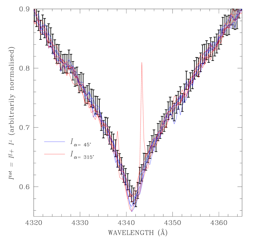
Figure 3: WD 2047+372, H$\gamma$ Balmer line: the sum of fluxes in the parallel and perpendicular beam split by the Savart plate, normalised to a pseudo-continuum, for all eight exposures obtained in the observing series, overplotted with the error bars.

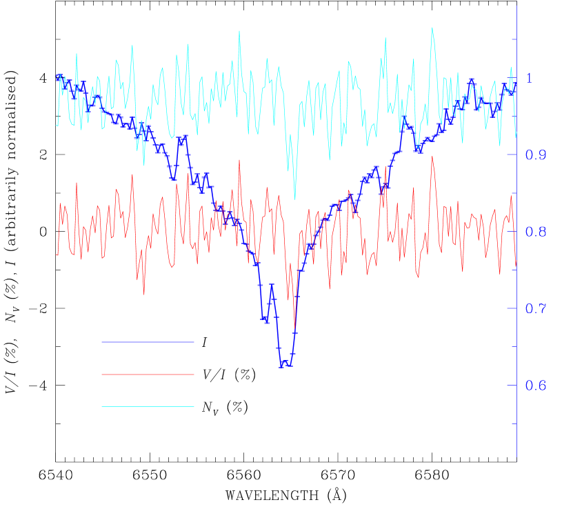
Figure 4: H$\alpha$ Stokes $I$ (blue solid line) and $V/I$ (red solid line) profiles of WD 2047+372 obtained with ISIS. The null profile is plotted with a solid light blue line, offset by $+3.5$ % for display purpose, and the left scale describes these data. The scale for the $I$ spectrum is on the right.

The field strength $\langle B_{z}\rangle$ was determined using the weak-field approximation,

$$V/I=-g_{\rm eff}C_{\rm z}\lambda^{2}\frac{1}{I}\frac{{\rm d}I}{{\rm d}\lambda}\langle B_{z}\rangle,$$ (3)

as the slope of the correlation line of the pixel-by-pixel circular polarisation $V/I$ as a function of the local value of $-g_{\rm eff}C_{z}\lambda^{2}(1/I)({\rm d}I/{\rm d}\lambda)$, a method discussed in detail by Bagnulo et al. (2002, 2012). As in Eq. (1), $g_{\rm eff}=1$ is the effective Landé factor of the Balmer lines, $g_{\rm eff}=1.25$ is assumed for the metal lines (Bagnulo et al. 2012), and $\lambda$ is the wavelength in Å units. Using this technique we measured the magnetic field from all H Balmer lines from H$\alpha$ to H9. As a quality check we also measured the magnetic fields from the null profiles. The results are presented in Table 1. Figure 5 shows our observations and the results of the least-square technique used for field determination on the H Balmer lines from H$\beta$ down to H$9$.

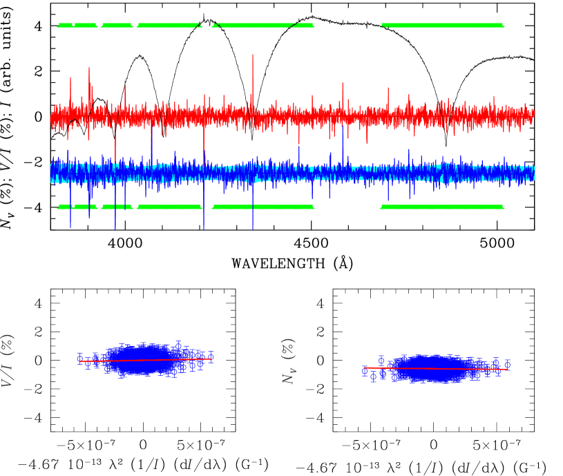
Figure 5: Spectropolarimetry of WD 2047+372. In the upper panel, the black solid line shows the intensity profile, the shape of which is heavily affected by the transmission function of the atmosphere + telescope optics + instrument. The zero level of intensity is very close to the bottom of the panel, at $-5$ on the left-hand scale. The red solid line is the reduced Stokes $V/I$ profile in % units. Photon-noise error bars are centred around $-2.5$ % and appear as a light blue background, to which the null profile (also offset by $-2.5$ % for display purpose) is superposed (blue solid line). The two bottom panels show the best-fit obtained by fitting with a straight line $V/I$ as a function of the quantity $\propto\lambda^{2}(1/I)\ \mathrm{d}I/\mathrm{d}\lambda)$. The green bars at the top and bottom of the upper panel show the spectral regions included in the correlation plots in the small lower panels.

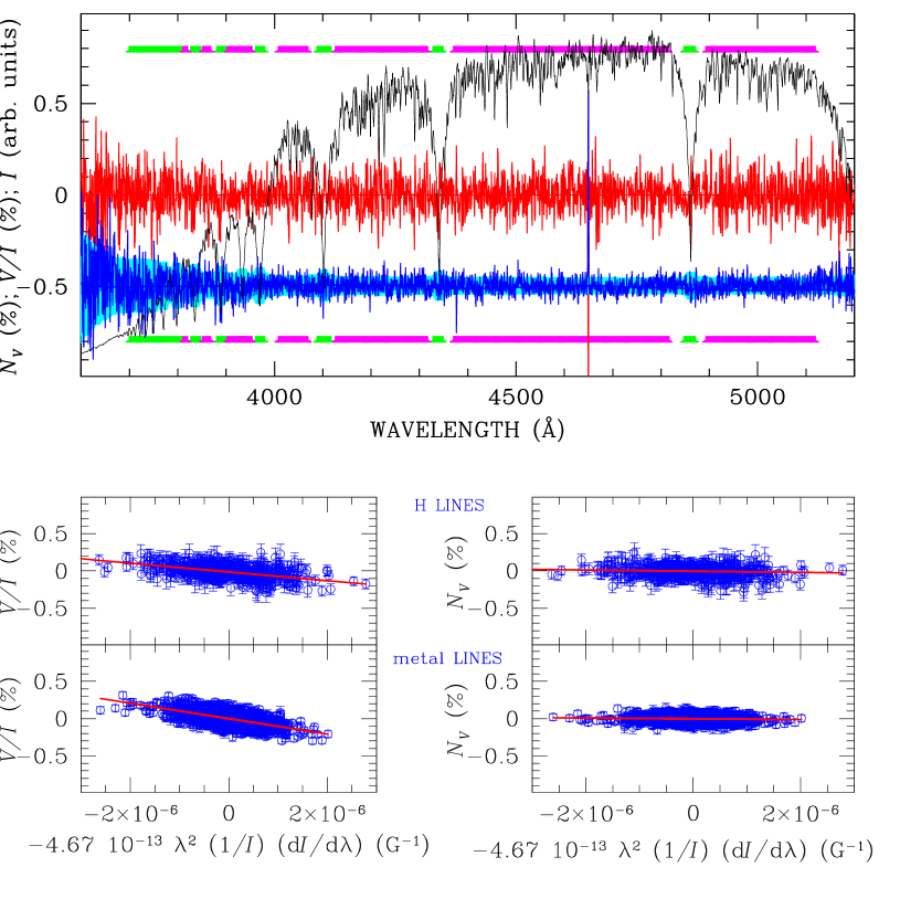
Figure 6: Same as Fig. 5 but for the magnetic Ap star $\gamma$ Equ. In the top panel, the magenta lines highlight the regions covered by metal lines that have been used for a further estimate of the magnetic field.

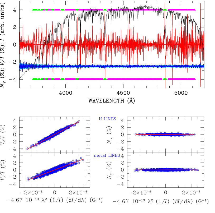
Figure 7: Same as Fig. 5 but for the magnetic Ap star HD 215441 (Babcock’s star).

Table 1: Magnetic field measurements for three stars obtained with the ISIS instrument.

Star:	WD 2047+372				HD 215441				HD 201601
Epoch:	2015-09-01 01:58 UT				2015-08-29 05:56 UT				2015-08-31 03:06 UT
Exp. time, peak S/N:	3360 s,   576  per Å				960 s,  1740  per Å				120 s,  3770  per Å
	$\langle B_{z}\rangle$ (G)		$\langle N_{z}\rangle$ (G)		$\langle B_{z}\rangle$ (G)		$\langle N_{z}\rangle$ (G)		$\langle B_{z}\rangle$ (G)		$\langle N_{z}\rangle$ (G)
H$\alpha$	$790$$\pm$	430	$910$$\pm$	400	$14160$$\pm$	71	$50$$\pm$	77	$-525$$\pm$	94	$39$$\pm$	32
H$\beta$	$940$$\pm$	1000	$185$$\pm$	960	$16525$$\pm$	300	$45$$\pm$	160	$-680$$\pm$	67	$-36$$\pm$	57
H$\gamma$	$490$$\pm$	1080	$-730$$\pm$	1200	$17550$$\pm$	230	$-20$$\pm$	170	$-700$$\pm$	70	$106$$\pm$	45
H$\delta$–H9	$+40$$\pm$	1070	$-75$$\pm$	1130	$18050$$\pm$	140	$-55$$\pm$	85	$-505$$\pm$	48	$-147$$\pm$	38
All H lines	$610$$\pm$	240	$-715$$\pm$	240	$17785$$\pm$	115	$-50$$\pm$	65	$-520$$\pm$	33	$-44$$\pm$	19
blue metal lines					$12510$$\pm$	100	$130$$\pm$	35	$-1036$$\pm$	30	$-50$$\pm$	15
red metal lines					$5090$$\pm$	170	$50$$\pm$	25	$-1050$$\pm$	20	$50$$\pm$	10

2.2.1 Other observations with ISIS

The ISIS instrument has not been extensively used as a magnetograph. To the best of our knowledge, the only ISIS field measurements reported in the literature are those by Leone (2007), who described a measurement of four magnetic Ap stars, and the paper by Landstreet et al. (2015), who reported observations of the white dwarf 40 Eri B. Therefore, in the course of our observing campaign, we have observed a number of well known magnetic stars and carried out a few experiments which will be discussed in detail in a forthcoming paper. Here we limit ourselves to discussing some observations obtained during the same run as WD 2047+372, which support the reliability of its field measurement.

During our run we observed the well known magnetic star HD 215441 (Babcock’s star), and the long period ($P\sim 100$ years!) magnetic star HD 201601 = $\gamma$ Equ. The results of our measurements are given in Table 1. They are globally consistent with previous literature data.

Of special interest is the case of HD 201601, for which the average of field measurements made using the metal line spectrum (i.e. excluding windows around each Balmer line from the analysis) is close to $\langle B_{z}\rangle\approx-1000$ G. The ensemble of more than 60 yr of $\langle B_{z}\rangle$ data available for the star, with many new measurements, has recently been studied by Bychkov et al. (2006, 2016), who fit a sine wave variation to all the available $\langle B_{z}\rangle$ values, most of which are based on analysis of spectropolarimetry of metal line spectra. They derive a rotation period of $97.16\pm 3.15$ yr, with zero point at the negative extremum that occurred on about JD 241 7795.0. (Note that in the ephemeris as described in Eqs (2) and (3) of Bychkov et al. (2016), the argument $\phi$ of the sine function in Eq. (2) should be replaced by $\phi-\pi/2$ in order for the new results to agree with the 2006 results.)

When their (corrected) new ephemeris and fitted sine wave parameters are used to compute the expected $\langle B_{z}\rangle$ value for our measurement, their ephemeris predicts $\langle B_{z}\rangle\approx-740$ G. This is (probably) significantly discrepant with our measurement of $-1000$ G. Since even the huge data set used by Bychkov et al. (2016) does not yet cover one full rotation cycle, the period that they find is certainly affected by scatter due to different instrumental systems of measurement of $\langle B_{z}\rangle$ (see Landstreet et al. 2014), which means that the uncertainty in the period that they derive, $\pm 3.15$ yr, is probably underestimated. Our measurement suggests that the true rotation period may be a few years, perhaps even a decade, longer than the period of Bychkov et al. (2016). However, the discrepancy could also arise because our instrumental measurement system for $\langle B_{z}\rangle$, even restricting ourselves to the value from the blue arm of ISIS, is significantly different from many of the other instrumental systems used to measure $\langle B_{z}\rangle$ in the past.

Note that the average of our Balmer line measurements of the field of $\gamma$ Equ, about $-520$ G, is consistent with the observation by Bychkov et al. (2016) that the values of $\langle B_{z}\rangle$ measured for HD 201601 using Balmer lines tend to have smaller amplitude than those measured using metal lines, and in fact our measurement is in good agreement with the recent $\langle B_{z}\rangle$ measurements of HD 201601 from dimaPol shown in Figure 6 of Bychkov et al. (2016).

Overall, our measurement of $\langle B_{z}\rangle$ for $\gamma$ Equ confirms that field measurements made with ISIS have the expected sensitivity and accuracy, and are consistent with measurements from other well-tested spectropolarimeters.

The observations of HD 215441 reveal a somewhat more complex result. Table 1 shows a general concordance among the Balmer line field values for HD 215441, but also a modest systematic increase in the detected field from H$\alpha$ to the upper Balmer lines. This systematic trend probably arises from the fact that different Balmer lines have different darkening and line weakening rates towards the limb, and thus weight the local $B_{z}(x,y)$ field differently from one another in the average over the visible hemisphere. However, the observed field strength is within the range of $\langle B_{z}\rangle$ values found (using the wings of the Balmer H$\beta$) for HD 215441 by Borra & Landstreet (1978). It is clear that the weak-field approximation of Eq. (3) used to measure $\langle B_{z}\rangle$ from the ISIS Balmer line spectrum is still valid for fields up to at least $\langle B_{z}\rangle\sim 20$ kG. Thus we are confident that Eq. (3) is also valid for the (weaker) $\langle B_{z}\rangle$ field measured in WD 2047+372, using still broader Balmer lines than those of HD 215441.

In contrast, there is a large discrepancy between $\langle B_{z}\rangle$ field measurements of HD 215441 obtained using metallic lines in the red and in the blue arm, and a smaller discrepancy between the blue arm metallic line $\langle B_{z}\rangle$ and the blue arm Balmer line $\langle B_{z}\rangle$. From the instrumental point of view, one could suspect that the retarder waveplate is affected by a chromatic problem, i.e., that the retardation is optimised for the blue region, and departs substantially from its nominal $\pi/4$ value at $\ga 6000$ Å. However, the consistency of the very precise red and blue arm metal line field values measured for $\gamma$ Equ suggests instead that the explanation for the observed discrepancy may be specific to the observed star rather than due to instrumental reasons. Babcock’s star has a very strong magnetic field, and the Zeeman splitting is totally resolved in many spectral lines, with $\pi-\sigma$ separations of more than 0.5 Å in some blue lines (Landstreet et al. 1989). In a spectrum with resolved Zeeman patterns, the peaks in $V$ no longer coincide with regions of large slope ${\rm d}I/{\rm d}\lambda$ in the line profile, but instead are largest where the two sigma components are strongest. Thus Eq. (3) ceases to be a useful approximation.

In a low resolution spectrum, instrumental broadening can recreate the weak-field situation of Eq. (3) by blending the Zeeman components together so that the (smoothed) peaks in $V$ still do coincide roughly with (smoothed) line wings in the $I$ spectrum. In the ISIS spectrum, the resolving power is larger in the red arm than in the blue arm, by a factor of about three. Furthermore, the typical Zeeman splitting, proportional to $\lambda^{2}$ (see Eq (1) is about twice as large in the red as in the blue arm spectra. As a result, the blue arm spectrum is still mostly in the weak-field regime with peaks in $V$ coinciding with line wings in $I$, while in the red arm spectrum this approximation has begun to break down seriously: many peaks in $V$ are more nearly coinciding with dips in $I$ than points of large slope ${\rm d}I/{\rm d}\lambda$. Thus the value of $\langle B_{z}\rangle$ derived with the weak-field approximation with the blue arm spectrum is only moderately smaller than values found using Balmer lines (which are certainly still in the weak-field regime), while $\langle B_{z}\rangle$ from the red arm falls well below the expected value.

The correctness of this argument is supported by analysis of a single high resolution ESPaDOnS spectrum; in that spectrum the $\langle B_{z}\rangle$ field strengths of about 15 kG derived from various parts of the spectrum using Eq. (2), and thus without using the weak-field approximation of Eq. (3), are all consistent.

3 The magnetic field of WD 2047+372

In the ESPaDOnS $I$ spectrum we see well-defined $\sigma$ components that are not significantly broader than the central $\pi$ component, quite unlike the situation of some other weak-field magnetic stars such as WD 2359$-434$, whose $\sigma$ components are clearly strongly broadened (cf. Landstreet et al. 2012). The narrowness of the $\sigma$ components in WD 2047+372 strongly suggests that the field at the time of the ESPaDOnS observation is relatively uniform in field modulus $\langle|B|\rangle$, and it may well be rather orderly. These data are consistent with a very simple field geometry, one which could be approximated by a uniform field in the hemisphere viewed at the time of the ESPaDOnS observation.

Both measurements of $\langle B_{z}\rangle$ give values of about $0.1\langle|B|\rangle$ or less. If we suppose that the field is approximately described by the oblique rotator model (a roughly axisymmetric field fixed in the star, with the magnetic axis inclined at an angle $\beta$ to the stellar rotation axis, which in turn is inclined by the angle $i$ to the line of sight), then the small value of $\langle B_{z}\rangle$ relative to $\langle|B|\rangle$ suggests that the line of sight is directed approximately towards the stellar magnetic equator, which would imply that at least one of $i$ or $\beta$ is large. However, further field measurements are required to establish whether this model is plausible or not.

Because we have two spectra of WD 2047+372, we can obtain some information about possible variability of the magnetic field. A comparison of the two H$\alpha$ $I$ spectra is shown in Figure 8. The ESPaDOnS spectrum here is binned to pixels of 0.25 Å to match the pixel spacing of the ISIS spectrum. The two Zeeman split line cores are similar in width, but the $\langle|B|\rangle$ field seems to have been slightly stronger at the time that the ISIS spectrum was obtained. More striking is the obvious difference in shape between the two line cores. It seems clear that the observed field strength or structure of WD 2047+372 is somewhat variable as the star rotates. The asymmetric form of the ISIS H$\alpha$ line core may be the result of a combination of a somewhat non-uniform field over the hemisphere viewed at the time of that observation, combined with the Doppler shifts associated with significant rotation velocity.

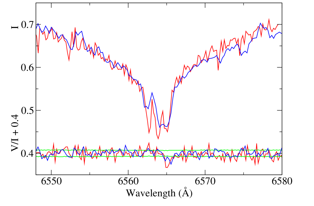
Figure 8: Comparison of the $I$ and $V/I$ spectra of the core of H$\alpha$ as observed with ISIS on 2015-09-01 (blue solid line), and as observed with ESPaDOnS on 2015-10-31 (red solid line). Both spectra have been normalised to 0.65 at 6555 Å. The $V/I$ spectra have been shifted upwards by $+0.4$ for ease of comparison with the $I$ spectra.

4 Discussion and Conclusions

The significance of the detection of this very weak field (“weak” for a white dwarf!) is that there are only two white dwarfs in which the presence of a still weaker magnetic field is clearly established by spectropolarimetry and observation of the H$\alpha$ line core broadening: WD 0446$-789$, with $\langle|B|\rangle\sim 20$ kG, and WD 2105$-820$, with $\langle|B|\rangle\approx 43$ kG (Koester et al. 1998; Aznar Cuadrado et al. 2004; Landstreet et al. 2012). It has been suggested that a very weak field is present in WD 1105$-048$ (Aznar Cuadrado et al. 2004), but our unpublished measurements have not yet clearly confirmed, or rejected, this result.

If we look at the current sample of white dwarfs for which fields have been firmly detected, and that show values of $\langle|B|\rangle$ that are always below 120 kG, which we list in Table 2, we can add only WD 1653$+385$, with $\langle|B|\rangle=70$ kG; WD 0257$+080$, with $\langle|B|\rangle\approx 90$ kG; WD 2359$-434$, with $\langle|B|\rangle\approx 110$ kG, and WD 0322$-019$, with $\langle|B|\rangle=120$ kG (Bergeron et al. 2001; Aznar Cuadrado et al. 2004; Koester et al. 2009; Gianninas et al. 2011; Zuckerman et al. 2011; Farihi et al. 2011). Thus WD 2047+372 is a valuable addition to the very small sample of the weakest known white dwarf magnetic fields. Furthermore, of these seven stars, even the most elementary magnetic and geometric model has been proposed for only one, WD 2105-820 (Landstreet et al. 2012).

Table 2: White dwarfs with confirmed fields $\langle|B|\rangle\leq 120$ kG

Star	$T_{\mathrm{eff}}$	$\langle B_{z}\rangle$ range	$\langle|B|\rangle$
	(K)	(kG)	(kG)
WD 0446$-789$	24440	–2.5 to –5.5	$\sim 20$
WD 2105$-820$	10600	$-8$ to $-11$	43
WD 2047$+372$	14710	$+2$ to $+6$	57
WD 1653$+385$	5900		70
WD 0257$+080$	6430	$\sim 35$	90
WD 2359$-434$	8650	3	110
WD 0322$-019$	5310		120

Summary lists of white dwarfs with weak magnetic fields have recently been published by Kawka & Vennes (2012); Ferrario et al. (2015). The most recent list, from Ferrario et al. (2015), contains 15 white dwarfs which are supposed to have magnetic fields below about 120 kG. Our list in Table 2 contains only seven stars. This is due to changes to the two recent lists, and to omission from our list of doubtful detections, as detailed below.

• Magnetic field detections in NLTT 347 = WD 0005-048, G234$-4$ = WD 0728+642, LB 8827 = WD 0853+163, LTT 4099 = WD 1105$-048$, WD 1531$-022$, G 226-29 = WD 1647+591, and WD 2039$-682$ are in fact currently unconfirmed, although some of these stars may eventually be shown to have some of the smallest white dwarf fields.

• 40 Eri B has been shown to be em non-magnetic at the level of about 250 G (Landstreet et al. 2015).

• The $\langle|B|\rangle$ value of LP 907$-37$ = WD 1350$-090$ was not measured by Koester et al. (1998), but it is found that $\langle|B|\rangle=460\pm 20$ kG from their spectrum.

• The field attributed to G 227-28 = WD 1820+609 is due to a typographical error in Putney (1997), who incorrectly recorded a non-detection measured by Liebert & Stockman (1980).

• WD 2329$-291$ is not a white dwarf but an sdB star (Gianninas et al. 2011).

• The $\langle|B|\rangle$ field of LTT 9857 = WD 2359$-434$ is not 9.8 kG but slightly exceeds 100 kG (Koester et al. 2009).

It seems very probable that the small number of very weak magnetic fields now known in white dwarfs is due to reaching the current practical detection threshold, as detecting fields so weak rapidly becomes increasingly difficult as one looks at fainter and fainter stars. In fact, four of the seven weak-field magnetic white dwarfs listed in Table 2 are brighter than $V=13.5$, and thus are among the brightest known magnetic white dwarfs.

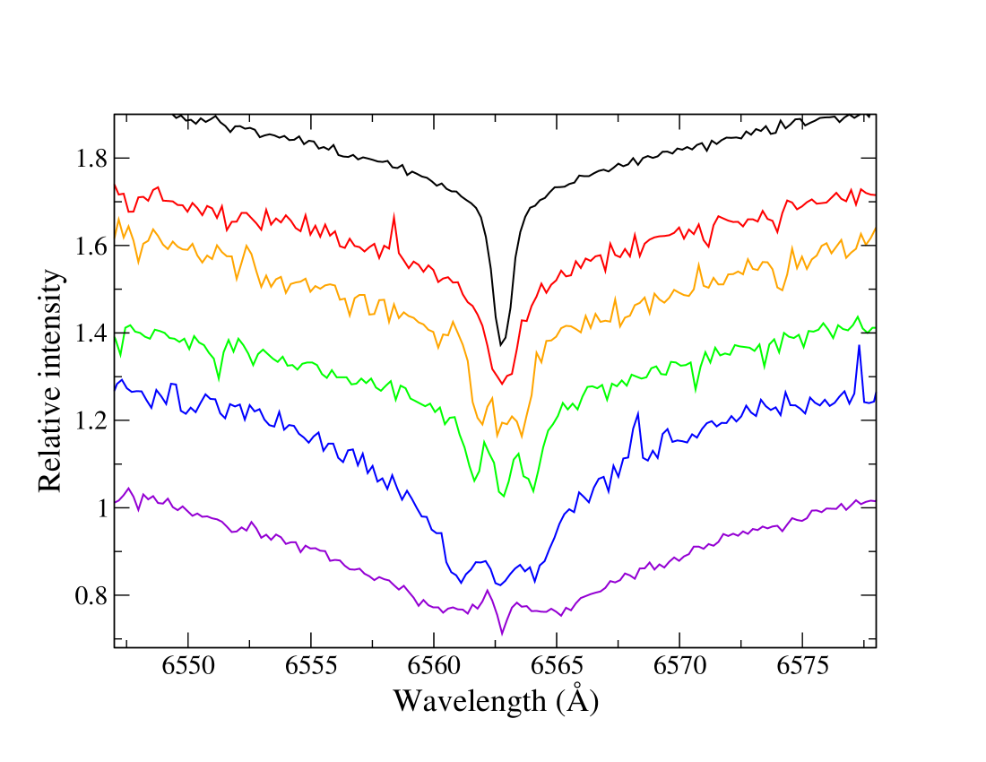
Figure 9: Comparison of the intensity spectra of a non-magnetic white dwarf (WD 2007$-303$, top) followed in order of increasing $\langle|B|\rangle$ by the DA stars WD 0446$-789$, WD 2105$-820$, WD 2047+372, WD 0257+080, and WD 2359$-434$. All spectra have been rebinned in bins of width 0.2 Å (in some cases two spectra have been averaged) to improve S/N in the plot, normalised to 1.0 at 6550 and 6575 Å, Doppler shifted to the rest frame of H$\alpha$, and then offset vertically for clarity.

We have available intensity spectra of five of the seven magnetic white dwarfs of Table 2 (the DA stars), mostly observed for the SPY project (Koester et al. 1998, 2009) and obtained from the ESO Archive. The appearance of H$\alpha$ in these stars is shown in Figure 9. It will be noticed that the rather well-defined Zeeman triplet of WD 2047+372 is unusual (and as mentioned above probably reflects a field geometry such that $|B|$ varies by only perhaps 20 or 30 % across the surface of the visible hemisphere). The weaker fields of WD 0446$-789$ and WD 2105$-820$ do not show clear resolution into components because the splitting is not large enough relative to the intrinsic width of the Zeeman components, while the larger fields of WD 0257+080 and WD 2359$-434$ are apparently rather non-uniform over the visible hemisphere, thus broadening the $\sigma$ (but not the $\pi$) components.

Our short list of five magnetic white dwarfs with $\langle|B|\rangle$ below 100 kG, of which three are brighter than $V=13.5$, makes it possible for us to estimate very roughly the fraction of white dwarfs in a magnitude-limited sample that have extremely weak magnetic fields. When we search the list of all white dwarfs in the Vizier catalogue of McCook & Sion, we find 67 DA white dwarfs. We have not yet searched all 60+ white dwarfs with the best currently possible uncertainties (nor has anyone else), but it already appears (with rather weak statistical significance) that at least about 3–4% of DA white dwarfs probably possess a very weak magnetic field, of the order of 10–100 kG, a situation previously suggested by Schmidt & Smith (1995).

The discovery of the very weak field of WD 2047+372 confirms that it is practical to detect and study magnetic fields in white dwarfs having $\langle B_{z}\rangle$ of the order of a few kG and $\langle|B|\rangle\ga 20$ kG with several currently available facility instruments, down to a limiting magnitude of the order of $V\sim 14-15$. We should thus soon have a well-observed sample of at least several stars at the presently observable low end of the distribution of white dwarf magnetic field strength which can be studied in detail for clues that they may yield about the origin and evolution of these fields.