High – Temperature Superconductivity in FeSe Monolayers

Abstract

This review discusses the main experiments and theoretical views related to observation of high – temperature superconductivity in intercalated FeSe compounds and single layer films of FeSe on substrates like SrTiO₃. We consider in detail the electronic structure of these systems, both theoretical calculations of this structure at hand and their correspondence with ARPES experiments. It is stressed that electronic spectrum of these systems is qualitatively different from typical picture of the spectrum in well studied FeAs superconductors and the related problems of theoretical description of spectrum formation are also discussed.

We also discuss the possible mechanisms of Cooper pairing in monolayers of FeSe and problems appearing here. As single layer films of FeSe on SrTiO₃ can be represented as typical Ginzburg “sandwiches”, we analyze the possibility of rising the critical temperature of superconducting transition $T_{c}$ due to different variants of “excitonic” mechanism of superconductivity. It is shown, that in its classic variant (as proposed for such systems by Allender, Bray and Bardeen) this mechanism is unable to explain the observed values of $T_{c}$, but situation is different when we consider instead of “excitons” the optical phonons in SrTiO₃ (with energy of the order of 100 meV). We consider both the simplest model of $T_{c}$ enhancement due to interaction with such phonons and more specific models with dominant “forward” scattering, which allow to understand the growth of $T_{c}$ as compared with the case of bulk FeSe and intercalated FeSe systems. We also discuss the problems connected with antiadiabatic nature of superconductivity due to such mechanism.

PACS: 74.20.-z, 74.20.Fg, 74.20.Mn, 74.20.Rp, 74.25.Jb, 74.62.-c, 74.70.-b

I Introduction

Discovery of the new class of superconductors based upon iron pnictides has opened the new perspectives in the studies of high – temperature superconductivity. While possessing the main superconducting characteristics somehow inferior to those of copper oxides (cuprates), these systems attracted much attention of researchers, as the nature of superconductivity and other physical properties here are in many respects different from those of cuprates, while preserving many common features, which leads to the hopes for more deep understanding of the problem of high – temperature superconductivity as a whole. And this problem, which was put into the agenda mainly due to the enthusiasm of V.L. Ginzburg VLG ; HTSC77 , still remains among the central problems of the modern physics of condensed matter.

At present the properties iron pnictide superconductors are rather well studied experimentally, there is also almost overwhelmingly accepted theoretical picture of superconductivity in these systems, which is based on the idea of leading role of pairing interaction due to exchange of (antiferro)magnetic fluctuations, which in most cases lead to $s^{\pm}$ pairing on different sheets of the Fermi surface, which appear in these multiple bands systems. There is a number of review papers with detailed presentation of modern experimental situation and basic theoretical concepts, used to describe these systems Sad_08 ; Hoso_09 ; John ; MazKor ; Stew ; Kord_12 .

Soon after the discovery of superconductivity in iron pnictides, it was followed by its discovery in iron chalcogenide FeSe, which attracted attention probably only due to the unusual simplicity of this compound, while its superconducting characteristics (under normal conditions) were rather modest ($T_{c}\sim$8K), and its electronic structure was quite similar to that in iron pnictides. However, this system was also thoroughly studied (cf. review in FeSe ).

Situation with iron chalcogenides undergone the major change with the appearance of intercalated FeSe systems, where the values of $T_{c}\sim$ 30-40K were obtained, and which attracted much attention because of their unusual electronic structure JMMM ; JTLRev . At present a number of such compounds are known with properties significantly different from traditional iron pnictides and which require the development of new theoretical understanding of mechanisms of superconductivity, as the traditional for pnictides picture of $s^{\pm}$-pairing is apparently not working here.

All these problems rather sharpened after the experimental observation of superconductivity with $T_{c}\sim$ 80-100K in monolayers of FeSe (epitaxial films), grown on SrTiO₃ substrate (and the number of similar compounds). At present we can speak of the “new frontier” in the studies of high – temperature superconductivity Boz2014 .

This small review is devoted to the description of the main experimental results on superconductivity in intercalated FeSe monolayers and single layer films of FeSe on substrates like SrTiO₃, and to discussion of a number of related theoretical problems, including the possible mechanisms leading to significant enhancement of $T_{c}$. It should be said, that here we remain with more questions, than answers, but this is what attracts most of the researchers to the studies of systems discussed in this review. This field develops very fast and we can not claim for the overwhelming discussion of all available literature. Our presentation will be necessarily on rather elementary (general physics) level, with the hope to make it understandable for nonspecialists. The references to many important works can be found in papers quoted below, many papers are not mentioned simple because of the limited space for the review. However, the author hopes that this review will be of interest to a wide community of Physics Uspekhi readers as a kind of introduction to this new field of research, especially in connection with centenary of great physicist — V.L. Ginzburg, whose ideas and views on the problem of high – temperature superconductivity had so much influence on everybody who is involved in this field.

II Main systems and experiments

II.1 Intercalated FeSe systems

In Fig. 1 (a) we show schematically the simplest crystal structures of iron based superconductors Sad_08 ; Hoso_09 ; John ; MazKor ; Stew ; Kord_12 ; FeSe . The common element here is the presence of FeAs or FeSe plane (layer), where ions of Fe form the simple square lattice, while ions of pnictogens (Pn – As) or chalcogens (Ch – Se) are placed in the centers of these squares, above and below the Fe plane in chess – board order. In Fig. 1 (b) the structure of this layer is shown in more details. Actually the electronic states of Fe ions in FePn(Ch) plane play decisive role in the formation of electronic properties of these systems and among them — superconductivity. In this sense these layers are quite similar to CuO₂ planes in cuprates (copper oxides) and these systems can be considered, in the first approximation, as quasi – two – dimensional, though the anisotropy in most of them may be not so strong. Below we shall mainly limit ourselves to such oversimplified picture and speak about the physics of FeSe planes (monolayers).

In Fig. 1 (b) arrows show direction of spins on Fe in antiferromagnetic structure, which is typically realized in stoichiometric state of FeAs based systems Sad_08 ; Hoso_09 ; John ; MazKor ; Stew ; Kord_12 , which are (in their ground state) antiferromagnetic metals. Antiferromagnetic ordering is destroyed under electron or hole doping, when superconducting phase just appear. In this sense the phase diagrams of systems under consideration are quite similar to phase diagrams of cuprates Sad_08 ; Hoso_09 ; John ; MazKor ; Stew ; Kord_12 . These phase diagrams at present are rather well studied. In FeSe systems, which will be considered below, the character of magnetic ordering is known not so well. Because of this, as well as due to the lack of space, we practically shall not discuss magnetic properties of FeSe systems.

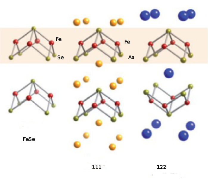
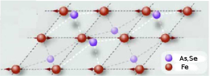
Figure 1: (a) – crystal structure of simplest iron based superconductors, (b) – structure of highly conducting plane (layer) of iron ions and pnictogens (chalcogens). Arrows show direction of spins for typical ordering in antiferromagnetic phase.

Note that all FeAs structures shown in Fig. 1 (a) are simple ionic – covalent crystals. The chemical formula say for typical 122 – system can be written, example, as Ba⁺²(Fe⁺²)₂(As^-3)₂. The charged FeAs layers are hold together by Coulomb forces from surrounding ions. In the bulk FeSe electroneutral FeSe layers are hold by much weaker van der Waals interactions. This makes this system convenient for intercalation by different atoms or molecules, which can easily enough penetrate between FeSe layers. The chemistry of intercalation of iron selenide superconductors is discussed in detail in a recent review VivRod .

As we already noted, superconductivity in bulk FeSe, discovered immediately after high – temperature superconductivity was observed in iron pnictides, was studied more or less in detail FeSe , but initially has not attracted much interest because of its similarity to superconductivity in iron pnictides and low enough superconducting characteristics. This situation changed drastically after the discovery of high – temperature superconductivity in intercalated FeSe compounds and especially after the achievement of record breaking values of $T_{c}$ in single layer films of FeSe on SrTiO₃.

First systems of this kind were A_xFe_2-ySe₂ (A=K,Rb,Cs) compounds, with the values of $T_{c}\sim$ 30K AFeSe ; AFeSe2 . It is commonly assumed that superconductivity here is realized in 122 – like structure shown in Fig. 2 (a), while real samples, studied up to now, were always multiphased, consisting of mesoscopic mixture of superconducting and insulating (antiferromagnetic) structures like K₂Fe₄Se₅, which naturally complicates the general picture. Significant further increase of $T_{c}$ up to the values of the order of 45K was achieved by intercalating the FeSe layers by large enough molecules in compounds like Li_x(C₂H₈N₂)Fe_2-ySe₂ intCH and Li_x(NH₂)_y(NH₃)_1-yFe₂Se₂ intNH . The increase of $T_{c}$ in these systems can be supposed to be related with the growth of spacing between FeSe layers from 5.5Å in bulk FeSe to $\sim$7Å in A_xFe_2-ySe₂ and to 8-11Å in systems intercalated by large molecules. i.e. with the growth of their two – dimensional nature.

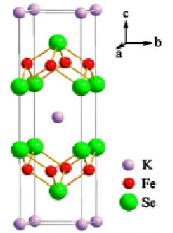
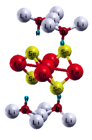
Figure 2: (a) – ideal ($x$=1) crystal structure (122 – type) of K_xFe₂Se₂ compound, (b) – ideal ($x$=0) crystal structure of [Li_1-xF_xOH]FeSe compound.

Recently the active studies has begun of [Li_1-xFe_xOH]FeSe system, where the values of $T_{c}\sim$ 43K were reached LiOH1 ; LiOH2 and it was possible to obtain rather good single – phase samples and single crystals. Crystal structure of this system is shown in Fig. 2 (b). An interesting discussion has developed on the nature of possible magnetic ordering on Fe ions replacing Li in intercalating layers of LiOH. In Ref. LiOH1 it was claimed that this ordering corresponds to a canted antiferromagnet. However, magnetic measurements of Ref. LiOH2 has lead to unexpected conclusion on ferromagnetic character of this ordering with Curie temperature $T_{C}\sim$ 10K, i.e. much lower than superconducting transition temperature. This conclusion was indirectly confirmed in Ref. LiOH3 by the observation of neutron scattering on the lattice of Abrikosov’s vortices, supposedly induced in FeSe layers by ferromagnetic ordering of spins of Fe in Li_1-xFe_xOH layers. At the same time, it was claimed in Ref. LiOH4 that Mössbauer measurements on this system indicate the absence of any kind of magnetic ordering on Fe ions.

II.2 Superconductivity in FeSe monolayer on SrTiO₃

The major breakthrough in the studies of superconductivity in FeSe systems, as already was noted above, is connected with the observation of record breaking values of $T_{c}$ in epitaxial films of monolayer of FeSe on SrTiO₃ (STO) substrate FeSe_STO1 . These films were grown in Ref. FeSe_STO1 and in most of the papers to follow on 001 plane of STO. The structure of these films is shown in Fig. 3, where we can see, in particular, that the FeSe layer is adjacent to TiO₂ layer on the surface of STO. Note that the lattice constant in FeSe layer of bulk samples is 3.77 Å, while in STO it is significantly larger being equal to 3.905 Å, so that the single layer FeSe films are noticeably stretched, as compared to the bulk FeSe and are in a stressed state, which disappears fast with addition of the next layers. Tunneling measurements of Ref. FeSe_STO1 has demonstrated the record values of the energy gap, while in resistance measurements the temperature of the onset superconducting transition essentially exceeded 50K. It should be stressed that films under study were quite unstable on the air, so that in most of the works resistive transitions were usually studied on films covered by amorphous Si or a number of layers of FeTe, which significantly reduced the observed values of $T_{c}$. The unique in situ measurements of FeSe films on STO, made in Ref. FeSe_STO2 , has given the record breaking values of $T_{c}>$ 100K, which can be seen from the data shown in Fig. 4. Up to now these results are not confirmed by other authors, but ARPES measurements of temperature behavior of energy gap in such films in situ at present routinely demonstrate the values of $T_{c}$ in the interval of 65-75 K.

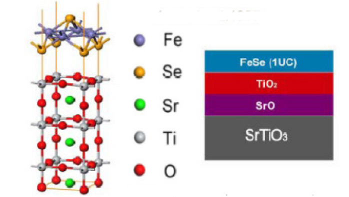
Figure 3: Structure of FeSe monolayer on SrTiO₃ substrate (001).

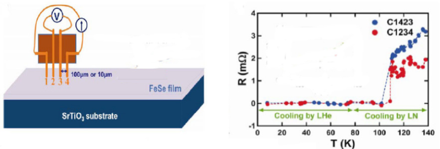
Figure 4: Experimental setup to measure resistance of single layer FeSe film on SrTiO₃ substrate and temperature dependence of resistivity obtained on two samples FeSe_STO2 .

In films consisting of several layers of FeSe the observed values of $T_{c}$ are significantly lower than record values of single layer films FeSe13UCK . Recently the monolayer FeSe films were grown also on 110 plane of STO FeSe_STO_FeTe , with cover up by several FeTe layers. Resistive measurements on these films (including the measurements of the upper critical magnetic field $H_{c2}$) has given the values of $T_{c}\sim$ 30 K. At the same time, FeSe films grown on BaTiO₃ (BTO), doped with Nb (with even larger values of the lattice constant $\sim$ 3.99Å), have shown (in ARPES measurements ) the values of $T_{c}\sim$70 K FeSe_BTO . A recent paper FeSe_Anatas has reported the observation of record (for FeSe systems) values of superconducting gap (from tunneling) in FeSe monolayers on 001 plane of TiO₂ (anatase), grown on 001 plane of SrTiO₃. It was noted that the lattice constants of anatase are quite close to those of the bulk FeSe, so that FeSe films is practically non stretched.

Single FeSe layer films were also grown on the graphene substrate FeSeGraph , but the values of $T_{c}$ of these films have not exceeded 8-10 K, characteristic of the bulk FeSe, which stresses the role of the substrates like Sr(Ba)TiO₃, with the unique properties, which may be determining for the strong enhancement of $T_{c}$.

We shall limit ourselves with this short review of experimental situation with observation of superconductivity in FeSe monolayers to concentrate below on the discussion of electronic structure and possible mechanisms, explaining the record (for iron based superconductors) values of $T_{c}$. More detailed information on experiments on this system can be found in a recent review FeSe1UC_rev .

III Electronic structure of iron – selenium systems

Electronic spectrum of iron pnictides is now well studied, both with theoretical calculations based on modern energy band theory and also experimentally, where the decisive role was played by ARPES experiments Sad_08 ; Hoso_09 ; John ; MazKor ; Stew ; Kord_12 . As we already noted above, almost all effects of interest to us are determined by electronic states of FeAs plane (layer), shown in Fig. 1 (b). The spectrum of carriers in the vicinity of the Fermi level (with the width $\sim$ 0.5 eV, where everything concerning superconductivity obviously takes place) is practically formed only by $d$-states of Fe. Hybridization of Fe and As states according to all band structure calculations is very small. Accordingly, up to five bands (two or three hole – like and two electron – like) cross the Fermi level, forming the spectrum typical for a semi – metal. The schematic picture of Brillouin zones and Fermi surfaces is shown in Fig. 5, and it is essentially rather simple.

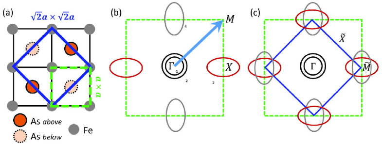
Figure 5: (a) – different choices of elementary cell in FeAs(Se) plane, (b) – Brillouin zone and Fermi surfaces for the case of one Fe ion in elementary cell, (c) – folded Brillouin zone and Fermi surfaces for the case of two Fe ions in elementary cell.

In first approximation, assuming that all As ions belong to the same plane as Fe ions, we have an elementary cell with one Fe and (square) lattice constant $a$ (cf. Fig. 5 (a)). Corresponding Brillouin zone is shown in Fig. 5 (b). If we take into account that As ions are in fact placed above and below Fe plane, as shown in Fig. 1 (b), the elementary cell will contain two Fe ions and Brillouin zone is reduced by a factor of two as shown in Fig. 5 (c). Two – dimensional Fermi surfaces for the case of four bands (two hole – like in the center and two electron – like at the edges or in the corners of appropriate Brillouin zones) are also schematically shown in Fig. 5 (b,c).

In the energy interval around the Fermi level, which is of interest to us, energy bands can be considered parabolic, so that the Hamiltonian of free carriers can be written as MazKor :

$$H=\sum_{{\bf k},\sigma,i=\alpha_{1},\alpha_{2},\beta_{1},\beta_{2}}\varepsilon^{i}_{\bf k}c_{i{\bf k}\sigma}^{\dagger}c_{i{\bf k}\sigma}.$$ (1)

where $c_{i{\bf k}\sigma}$ is annihilation operator of an electron with momentum and spin ${\bf k}$, $\sigma$ and band index $i$, and the hole bands $\alpha_{i}$ dispersions take the form:

$$\varepsilon^{\alpha_{1,2}}_{\bf k}=-\frac{k^{2}}{2m_{1,2}}+\mu$$ (2)

while the electron bands $\beta_{i}$ dispersions are written (in the coordinates of Brillouin zone of Fig. 5 (b)) as:

$$\varepsilon^{\beta_{1}}_{\bf k}=\frac{(k_{x}-\pi/a)^{2}}{2m_{x}}+\frac{k_{y}^{2}}{2m_{y}}-\mu$$

$$\varepsilon^{\beta_{2}}_{\bf k}=\frac{k_{x}^{2}}{2m_{y}}+\frac{(k_{y}-\pi/a)^{2}}{2m_{x}}-\mu$$ (3)

More complicated band structure models valid in the vicinity of the Fermi level and being in direct correspondence with LDA calculations can also be proposed (see e.g. KuchSad10 ), but the general, rather simple, picture of this “standard model” of iron pnictides spectrum remains the same. LDA+DMFT calculations DMFT1 ; DMFT2 , taking into account the role of electron correlations, show that in iron pnictides, in contrast to cuprates, this role is rather irrelevant and reduced to (actually noticeable) renormalization of the effective masses of electron and hole dispersions, as well to the general “compression” (reduced width) of the bands.

The presence of electron and hole Fermi surfaces with close sizes, satisfying (approximate!) “nesting” conditions, is very significant for the theories of superconducting pairing in iron pnictides based on the decisive role of antiferromagnetic spin fluctuations MazKor . Below we shall see that electronic spectrum and Fermi surfaces in Fe chalcogenides are significantly different from the qualitative picture presented above, which poses new (and far from being solved) problems of explaining the microscopic mechanism of superconductivity in these systems.

III.1 A_xFe_2-ySe₂ system

LDA calculations of electronic spectrum of A_xFe_2-ySe₂ (A=K,Cs) system were performed immediately after its experimental discovery KFe2Se2 ; KFe2Se2SI . Rather unexpectedly this spectrum was found to be qualitatively different from the spectrum of bulk FeSe and the spectra of all the known FeAs systems. In Fig. 6 we compare the spectrum of BaFe₂As₂ (Ba122) Ba122 , which is typical for all FeSe based systems, and the spectrum of A_xFe_2-ySe₂ (A=K,Cs), obtained in Ref. KFe2Se2 . We can see the clear difference of these spectra in the vicinity of the Fermi level.

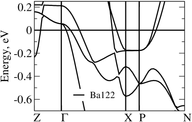
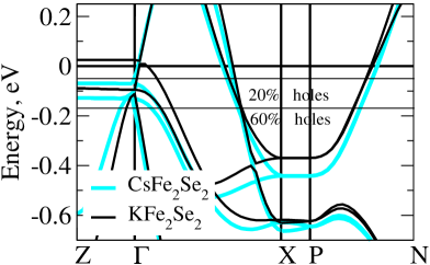
Figure 6: (a) – LDA bands of Ba122 close to the Fermi level ($E=$0) Ba122 , (b) – LDA bands of K_xFe₂Se₂ (black lines) and Cs_xFe₂Se₂ (blue lines). Additional horizontal lines correspond to Fermi level at 20% and 60% hole doping KFe2Se2 .

In Fig. 7 we show the Fermi surfaces calculated in Ref. KFe2Se2 for two typical compositions of A_xFe_2-ySe₂ (A=K,Cs). We can see that these are quite different from the Fermi surfaces of FeAs systems — in the center of Brillouin zone there are only small (electron – like!) Fermi surfaces, while electron – like cylinders at the corners of Brillouin zone are much larger. The shape of Fermi surfaces typical for the bulk FeSe and FeAs based systems is reproduced only for much larger (unreachable) hole doping levels KFe2Se2 .

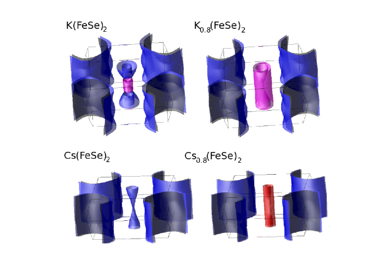
Figure 7: Fermi surfaces of A_xFe₂Se₂ (A=K,Cs) for stoichiometric composition and for the case of 20% hole doping KFe2Se2 .

This form of the Fermi surfaces in A_xFe_2-ySe₂ was soon confirmed by ARPES experiments. As an example, in Fig. 8 we show ARPES data of Ref. KFe2Se2ARPES , which are in obvious qualitative correspondence with LDA calculations KFe2Se2 ; KFe2Se2SI .

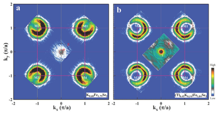
Figure 8: ARPES Fermi surfaces of K_0.68Fe_1.79Se₂ ($T_{c}$=32K) and Tl_0.45K_0.34Fe_1.84Se₂ ($T_{c}$=28K) KFe2Se2ARPES .

It is seen that in this system we can not speak of any, even approximate, “nesting” properties of electron – like and hole – like Fermi surfaces, while it is precisely these properties that form the basis of the most of theoretical approaches to microscopic description of FeAs based systems MazKor , where “nesting” of electron – like and hole – like Fermi surfaces leads to the picture of well developed spin fluctuations, which are considered as the main mechanism of pairing interaction.

LDA+DMFT calculations of K_1-xFe_2-ySe₂ for different doping levels were performed in Refs. KFeSeLDADMFT1 ; KFeSeLDADMFT2 . There, besides the standard LDA+DMFT approach we have used also the modified LDA^′+DMFT developed by us in Refs. CLDA ; CLDA_long , which allows, in our opinion, the more consistent solution of the “double – counting” problem of Coulomb interactions in LDA+DMFT. For DMFT calculations we have chosen the $U=3.75$ eV and $J=0.56$ eV as the values of Coulomb and exchange interactions in 3$d$ shell of Fe. As impurity solver we have used the Quantum Monte – Carlo (QMC). The results of these calculations were directly compared with ARPES data of Refs. KFe2Se2_ARPES ; KFe2Se2_ARPES_2 .

It can be seen that for K_1-xFe_2-ySe₂ system the correlation effects play rather significant role. They lead to noticeable change of LDA dispersions. In contrast to iron arsenides, where the quasi – particle bands close to the Fermi level remain well defined, in K_1-xFe_2-ySe₂ compounds, in the vicinity of the Fermi level we observe rather strong suppression of quasi – particle bands. This reflects the fact, that correlation effects in this system are more strong, than in iron arsenides. The value of correlation renormalization (correlation narrowing) of the bands close to the Fermi level is given by the factor of 4 or 5, while in iron arsenides this factor is usually of the order of 2 or 3, for the same values of interaction parameters.

Results of these calculations are in general qualitative agreement with ARPES data of Refs. KFe2Se2_ARPES ; KFe2Se2_ARPES_2 , which also demonstrate the strong damping of quasi – particles in the immediate vicinity of the Fermi level and stronger renormalization of effective masses in comparison to FeAs systems. At the same time, our calculations do not reveal the formation of unusually “shallow” ($\sim$ 0.05 eV deep below the Fermi level) electron – like band at the $X$ point in Brillouin zone, which was observed in ARPES experiments.

III.2 [Li_1-xFe_xOH]FeSe system

In Ref. LiOHFeSe_NS we have performed LDA calculations of stoichiometric LiOHFeSe compound, the appropriate results for energy dispersions are shown in Fig. 9 (a). On a first sight the energy spectrum of this system is quite analogous to the spectra of the majority of FeAs systems and that of the bulk FeSe. In particular, the main contribution to the density of states in rather wide energy region around Fermi level comes from $d$-states of Fe, while the Fermi surfaces qualitatively have the same form as in the majority of Fe based superconductors. However, this impression is wrong — in real [Li_0.8Fe_0.2OH]FeSe superconductor, the partial replacement of Li by Fe in intercalating LiOH layers leads to significant electron doping, so that the Fermi level goes upward in energy (as compared to stoichiometric case) by 0.15 – 0.2 eV. Then, as it is clear from Fig. 9 (a) hole – like bands in the vicinity of $\Gamma$ point move below the Fermi level, so that hole – like cylinders of the Fermi surface just vanish. The general form of the Fermi surfaces for such electron doping level following from LDA calculations is shown in Fig. 9 (b) and it has much in common with similar results for A_xFe_2-ySe₂ system (cf. Fig. 7). This conclusion is confirmed by direct ARPES experiments LiOHFeSe_ARP , the results of these are shown in Fig. 9 (c).

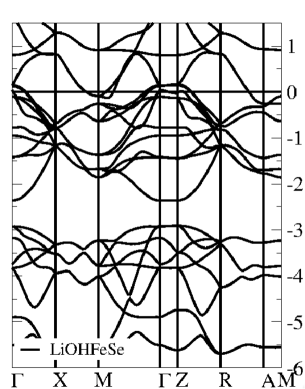
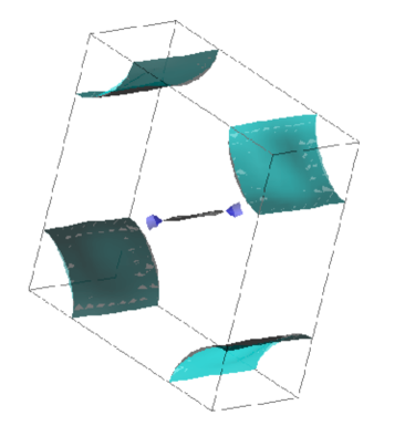
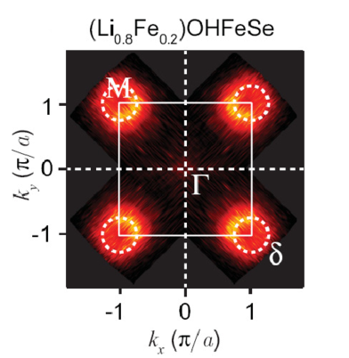
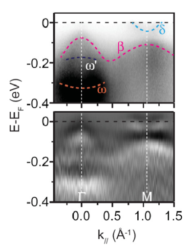
Figure 9: (a) – LDA bands of LiOHFeSe (Fermi level at $E=$0) LiOHFeSe_NS , (b) – Fermi surface of LiOHFeSe corresponding doping level of 0.3 electrons per unit cell, (c) – ARPES Fermi surfaces of [Li_0.8Fe_0.2OH]FeSe LiOHFeSe_ARP , (d) – ARPES bands close to the Fermi level in [Li_0.8Fe_0.2OH]FeSe LiOHFeSe_ARP .

In particular, we can see from Fig. 9 (b) that Fermi surfaces consist mainly of electron – like cylinders around points $M$, while in the vicinity of $\Gamma$ point Fermi surface is either absent or is quite small. In any case for this system there are no “nesting” properties between electron and hole surfaces in any sense. Electronic dispersions determined from ARPES are quite similar to corresponding dispersions measured in Refs. KFe2Se2_ARPES ; KFe2Se2_ARPES_2 for K_1-xFe_2-ySe₂ system. These are qualitatively similar to dispersions obtained in LDA calculations, taking into account strong enough correlation narrowing of bands (compression factor is actually different for different bands, as was shown by LDA+DMFT calculations of Refs. KFeSeLDADMFT1 ; KFeSeLDADMFT2 ). At the same time the origin of unusually “shallow” electronic band $\sim$ 0.05 eV deep eV close to $M$ point remains unclear. To explain this we need unusually strong correlation narrowing (while conserving the diameter of electron – like cylinders around the $M$ point, which practically coincides with the results of LDA calculations), which is difficult to obtain from LDA+DMFT calculations.

In Ref. LiOHFeSe_NS LSDA calculations of exchange parameters were performed for different configurations of Fe ions, replacing Li in LiOH layers. For most probable configuration, leading to magnetic ordering, the positive (ferromagnetic) sign of exchange interaction was obtained and the simplest estimate of Curie temperature has given the value of $T_{C}\approx$ 10K, in excellent agreement with experimental data of Refs. LiOH2 ; LiOH3 , which reported the observation of ferromagnetic ordering of Fe in LiOH layers. At the same time, as we mentioned above, the other experiments had cast some doubts on this conclusion.

III.3 FeSe monolayer

Calculations of LDA spectra of single layer of FeSe can be done in a standard way FNT_2016 . The results of such calculations are shown in Fig. 10 (a). It is seen that the spectrum looks like the typical for FeAs systems and the bulk FeSe, which was discussed in detail above. However, the ARPES experiments ARP_FS_FeSe_1 ; ARPES_FeSe_Nature ; ARP_FS_FeSe_2 had shown convincingly that this is not so. In monolayer of FeSe on STO only electron – like Fermi surfaces are observed around points $M$ in Brillouin zone, while hole – like sheets around $\Gamma$ point (at the zone center) are just absent. An example of this type of data is shown in Fig. 11 (a) ARP_FS_FeSe_1 . Thus, similarly to the case of intercalated FeSe systems, any kind of “nesting” properties are absent here. The apparent contradiction with the results of LDA calculations has a simple qualitative explanation — the observed Fermi surfaces can be easily obtained assuming that the system is electron doped, so that the Fermi level moves upward in energy by $\sim$ 0.2 – 0.25 eV, as shown by the red horizontal line in Fig. 10 (a). This corresponds to doping level of the order of 0.15 – 0.2 per Fe ion.

Strictly speaking, the origin of this doping remains unclear, but there is a general consensus that it is related to formation of oxygen vacancies in SrTiO₃ substrate (in TiO₂ layer), appearing during different technological operations (like annealing, etching etc.) used during the growth of the films under study . It should be noted that the formation of electron gas at the interface with SrTiO₃ is well known and was studied for rather long time Shkl_16 . However, for FeSe/STO system of interest to us, this problem was not studied in any detail (cf. though Refs. Mills ; Agter ).

Electronic correlations influence of the spectrum of single layer of FeSe is relatively weak. In Fig. 10 (b) we show the results of LDA+DMFT calculations for the case of appropriately shifted (by electron doping) Fermi level FNT_2016 . DMFT calculations were performed for the values of Coulomb and exchange (Hund – like) interactions strength in 3$d$ shell of Fe, taken as $U=3.5$ eV and $J=0.85$ eV. As impurity solver we have used here the continuous – time quantum Monte – Carlo (CT–QMC), and dimensionless inverse temperature was taken to be $\beta$=40. We can see that the spectrum is only weakly renormalized by correlations and conserves LDA – like form with rather low bandwidth compression factor $\sim$ 1.3.

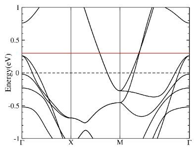
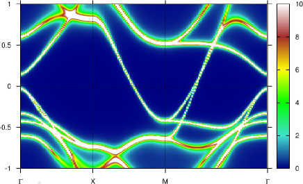
Figure 10: (a) – LDA bands of the single layer of FeSe close to the Fermi level ($E=$0). Horizontal red line denotes the approximate position of the Fermi level, corresponding to electron doping level leading the Fermi surfaces observed in ARPES experiments FNT_2016 , (b) – LDA+DMFT calculated bands of single layer of FeSe close to the Fermi level shifted by electron doping FNT_2016 .

Electronic dispersions in FeSe monolayer films were measured by ARPES in a number of works, e.g. in Refs. FeSe_BTO ; ARPES_FeSe_Nature . Results of Ref. ARPES_FeSe_Nature are presented in Fig. 11 (b). These are in agreement with data obtained in other papers and are, in general, analogous to the similar data obtained for intercalated FeSe systems (cf. e.g. Fig. 9 (c)). In general, these data are also qualitatively similar to the results of LDA+DMFT, but the quantitative agreement is absent. In particular, ARPES experiments clearly demonstrate the presence of unusually “shallow” electron – like band at the $M$ point, with Fermi energy $\sim$ 0.05 eV, while in theoretical calculations this band is almost an order of magnitude “deeper”.

It should also be noted that in Ref. ARPES_FeSe_Nature it was observed for the first time, that a “shadow” electron – like band exists at $M$ point, which is about 100 meV below the main band and is a kind of a “replica” of this band. This band is clearly seen in Fig. 11 (b). Such a “shadow” band is absent in band structure calculations. The nature of this band and its possible significance for high – temperature superconductivity in monolayers of FeSe on STO will be discussed in some detail below, in connection with possible mechanisms of enhancement of $T_{c}$.

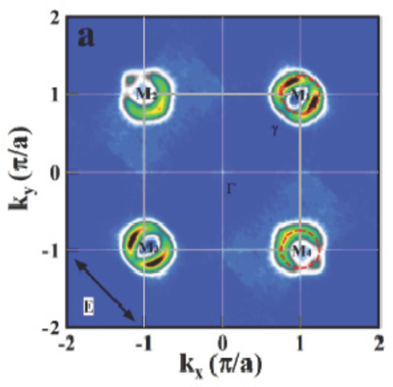
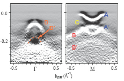
Figure 11: (a) – ARPES Fermi surface of single layer of FeSe ARP_FS_FeSe_1 , (b) – ARPES bands of FeSe single layer close to the Fermi level ARPES_FeSe_Nature .

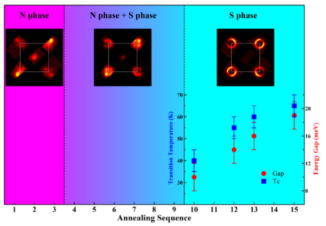
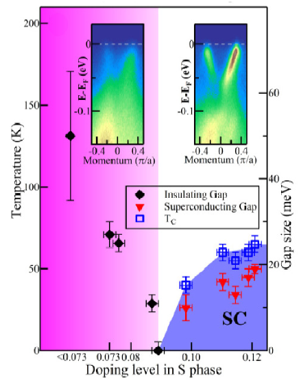
Figure 12: Phase diagram of FeSe single layer on SrTiO₃: (a) – schematic phase diagram obtained in Ref. FeSe1UC_Ph_Dia1 on the series of samples with different electron dopings. Also shown are corresponding ARPES Fermi surfaces and in superconducting phase ARPES measured values of superconducting gap and $T_{c}$. (b) – phase diagram obtained from ARPES measurements in Ref. FeSe1UC_Ph_Dia2 and demonstrating the existence of insulating and superconducting phases. The values of superconducting and insulating gaps were also obtained from ARPES measurements.

As we noted above electron doping level of FeSe monolayers on STO is rather poorly controlled parameter. However, in a number of papers, using different procedures of film annealing in situ, the authors successfully made ARPES experiments on samples with different doping levels FeSe1UC_Ph_Dia1 ; FeSe1UC_Ph_Dia2 . These experiments allowed to obtain some kind of phase diagrams of FeSe/STO system. In particular, in Ref. FeSe1UC_Ph_Dia1 a series of samples was demonstrated with consequent transitions from the topology of the Fermi surface typical of FeAs systems and bulk FeSe (with Fermi surface sheets around $\Gamma$ point in the center of Brillouin zone) to topology of Fermi surface sheets around $M$ point. It was shown, that superconductivity with high $T_{c}$ appears only in samples without central Fermi surface sheets, while the samples with typical Fermi surface topology remain in the normal phase. Schematically these results are shown in Fig. 12 (a). The presence of superconductivity was determined from ARPES measurements of the energy gap at the Fermi level, and $T_{c}$ was derived from the temperature dependence of the gap.

In Ref. FeSe1UC_Ph_Dia2 similar measurements were done with electron concentration controlled by by measurements of the area of electron pockets of the Fermi surface around $M$ points. The obtained phase diagram is shown in Fig. 12 (b), where we see insulating (antiferromagnetic?) phase at low doping levels and superconducting phase at dopings exceeding the critical value $\sim$ 0.09, corresponding to the quantum critical point. These conclusions are also based on ARPES measurements of superconducting and insulating energy gaps in the spectrum and their temperature dependencies.

It is obvious that the results of Refs. FeSe1UC_Ph_Dia1 ; FeSe1UC_Ph_Dia2 are in some contradiction with each other, in particular, the nature of insulating phase observed in FeSe1UC_Ph_Dia2 remains unclear.

IV Possible mechanisms of $T_{c}$ enhancement in iron – selenium monolayers

IV.1 Correlation of $T_{c}$ and the density of states

Let us now start discussing the mechanisms of high – temperature superconductivity in systems under consideration. Concerning FeAs based superconductors there is general consensus in the literature. Electron – phonon mechanism of Cooper pairing is considered to be insufficient to explain the high values of $T_{c}$ in these systems Sad_08 and the preferable mechanism is assumed to be the pairing due to exchange of antiferromagnetic fluctuations. The repulsive nature of this interaction leads to the picture of $s^{\pm}$–pairing with different signs of superconducting order parameter (gap) $\Delta$ on hole – like (around the $\Gamma$ point at the center of Brillouin zone) and hole – like (around $M$ points in the corners of the zone) sheets of the Fermi surface MazKor . However, when we consider the systems based on monolayers of FeSe, this picture obviously becomes inconsistent — the observed topology of Fermi surfaces with complete absence of any “nesting” electron – like and hole – like sheets or even with total absence of hole – like Fermi surfaces clearly contradicts this picture. There is simply no obvious way to form well developed spin (antiferromagnetic) fluctuations. Thus, we shall start with the elementary analysis based on simple BCS model.

In Ref. hPn2 an interesting empirical dependence was discovered between the temperature of superconducting transition T_c in FeAs and FeSe systems and the height of the anion (As or Se) $\Delta z_{a}$ above the Fe plane (layer) (cf. Fig. 1). A sharp maximum of $T_{c}$ was observed for systems with $\Delta z_{a}\sim$1.37Å. In Refs. JMMM ; Kucinskii10 we presented the results of systematic LDA calculations of the total density of states at the Fermi level $N(E_{F})$ for a wide choice of (stoichiometric) FeAs and FeSe based systems with different values of $\Delta z_{a}$ (cf. Table 1). The obtained non – monotonous dependence of the density of states on $\Delta z_{a}$, shown in Fig. 13 (circles), which is determined by hybridization effects, in principle, is sufficient to explain the corresponding dependence of $T_{c}$.

Table 1: Total LDA calculated density of states N(E_F) and the values of T_c for iron based superconductors.

	$\Delta z_{a}$, Å	N(EF),	T${}^{BCS}_{c}$, K	T${}_{c}^{exp}$, K
		states/cell/eV
LaOFeP	1.130	2.28	3.2	6.6
Sr4Sc2O6Fe2P2	1.200	3.24	19	17
LaOFeAs	1.320	4.13	36	28
SmOFeAs	1.354	4.96	54	54
CeOFeAs	1.351	4.66	48	41
NdOFeAs	1.367	4.78	50	53
TbOFeAs	1.373	4.85	52	54
SrFFeAs	1.370	4.26	38	36
BaFe2As2	1.371	4.22	38	38
CaFFeAs	1.420	4.04	34	36
CsFe2Se2	1.435	3.6	29	27
KFe2Se2	1.45	3.94	34	31
LiOHFeSe	1.485	4.14	36	43
LiFeAs	1.505	3.86	31	18
FeSe	1.650	2.02	3	8

Corresponding dependence of $T_{c}$ on $\Delta z_{a}$ can be easily estimated along the lines of elementary BCS model, using the usual expression $T_{c}=1.14\omega_{D}e^{-1/\lambda}$, taking into account that $N(E_{F})$ directly enters dimensionless pairing interaction constant $\lambda=gN(E_{F})$ (where $g$ is corresponding dimensional coupling constant). Taking, rather arbitrary value $\omega_{D}$=350 K (which may be related to characteristic value of phonon frequencies in FeAs systems Sad_08 ) we can determine the value of $g$ fitting experimental value of $T_{c}$, e.g. for Ba122 system ($\sim$ 38 K), which gives $\lambda$=0.43. Fixing this value of $g$, we can easily recalculate the values of $T_{c}$ for all other systems, just taking appropriate values of the density of states from LDA calculations (cf. Fig. 13). Corresponding values of $T_{c}$ given in Table 1 and shown in Fig. 13 (stars) are in very reasonable agreement with experimental values, shown in the same Figure (triangles), which are also given in Table 1.

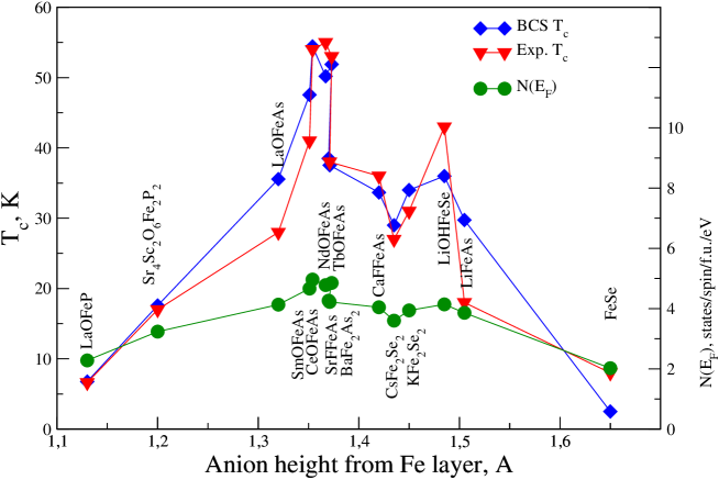
Figure 13: LDA calculated values of the density of states at the Fermi level $N(E_{F})$ (circles, right axis) and superconducting critical temperature $T_{c}$ (left axis), obtained from elementary BCS – like estimates (stars) and experimental values of $T_{c}$ (triangles) as functions of anion height $\Delta z_{a}$ over Fe layer for different iron based superconductors.

FeSe systems in general just fit this dependence. This can be seen from the data of Table 1 and Fig. 13. For example for [Li_1-xFe_xOH]FeSe system the calculated value of the density of states for stoichiometric composition LiOHFeSe is $N(E_{F})$=4.14 states/cell/eV and elementary estimate of $T_{c}$ yields T_c=36K, which is somehow lower than the experimental value $T_{c}$=43K. However, introduction of Fe into LiOH layers shifts the Fermi level, so that it moves to a higher value of $N(E_{F})$=4.55 states/cell/eV , leading to the appropriate growth of $T_{c}$ up to 45K, which is very close to experimental value LiOHFeSe_NS .

It should be stressed that the rough estimates given above does not necessarily mean that we assume electron – phonon pairing mechanism for these systems, and $\omega_{D}$ in BCS expression can be considered just as a characteristic frequency of any kind of Boson excitations responsible for pairing (e.g. magnetic fluctuations). These results show that there is an obvious correlation between experimental values of $T_{c}$ and the value of the total density of states at the Fermi level, obtained via band structure calculations for stoichiometric (!) compositions of FeAs and FeSe based compounds. Similar results can be obtained using more complicated expressions for $T_{c}$ like McMillan or Allen – Dynes formulas Kucinskii10 .

At the same time, for the single layer of FeSe LDA calculations produce the value $N(E_{F})\approx$ 2 states/cell/eV, which is practically the same as for the bulk FeSe and is weakly changing with electron doping (Fermi level shift) FNT_2016 . Corresponding elementary estimate of $T_{c}$ does not produce the values higher than 8K, so that the appearance of high values of $T_{c}$ in this case can not be explained from similar simple considerations.

However, there is a number of experimental papers, where the significant increase of $T_{c}$ were reported up to the values of the order of 40K in bulk crystals and multilayer films of FeSe under electron doping, achieved by the coverage of the surface of FeSe by alkali metal atoms (sodium) K_dop_1 ; K_dop_2 ; K_dop_3 . It is possible that this treatment has lead to intercalation of FeSe layers by alkali metal, so that these systems were transformed into an analogue of intercalated FeSe systems, similar to those discussed above, and the growth of $T_{c}$ was related to the growth of $N(E_{F})$. This point of view is confirmed by calculations presented in Ref. K_dop_band . However, the growth of $T_{c}$ up to the values $>$ 40K in a number of papers was achieved by doping of FeSe induced by strong electric field (at the gate) in the field – effects transistor structures Field_1 ; Field_2 ; Field_3 , where similar explanation seems less probable.

IV.2 Multiple bands picture of superconductivity

The basic feature of electronic spectrum of iron pnictide and chalcogenide superconductors is its multiple band character — in general case the Fermi level is crossed by several bands, formed by $d$ – states of Fe, so that there appear several sheets (pockets) of the Fermi surface (electron and hole – like) Sad_08 ; MazKor ; Kord_12 . In superconducting state the energy gap can open on each of these sheets and the values of these gaps can be quite different from each other Sad_08 ; Kord_12 . Thus, the elementary description of superconductivity based on the single – band BCS model used in the previous section is in fact oversimplified. Below, following mainly Refs. BGrk ; KucSad08 we shall briefly describe the multiple – band formulation of BCS model with application to Fe based superconductors.

Consider the simplified version of electronic structure (Fermi surfaces) of the square lattice of Fe, shown in Fig. 5 (b), with two hole – like pockets around the $\Gamma$ point and two electron – like pockets around $X$ and $Y$ points (in Brillouin zone for the square lattice with one Fe ion per unit cell). Let $\Delta_{i}$ denotes superconducting order parameter (energy gap) on $i$-th sheet (pocket) of the Fermi surface (in Fig. 5 (b) $i$=1,2,3,4). The value of $\Delta_{i}$ is determined by self – consistency equation for corresponding anomalous Green’s function in Gorkov’s system of equations BGrk .

Pairing interaction in multiple – band BCS model can be written in the matrix form:

$$\hat{V}=\left(\begin{array}[]{cccc}u&w&t&t\\ w&u^{\prime}&t^{\prime}&t^{\prime}\\ t&t^{\prime}&\lambda&\mu\\ t&t^{\prime}&\mu&\lambda\end{array}\right).$$ (4)

where matrix elements $V^{i,j}$ determine intraband and interband coupling constants. For example, $\lambda=V^{eX,eX}=V^{eY,eY}$ determines the pairing interaction on the same electron – like pocket at $X$ or $Y$ points, while $\mu=V^{eX,eY}$ connects electrons on different pockets at $X$ and $Y$. Constants $u=V^{h1,h1}$, $u^{\prime}=V^{h2,h2}$ and $w=V^{h1,h2}$ characterize BCS interaction on hole – like pockets — the smaller one ($h1$) and larger one ($h2$), and between them, while $t=V^{h,eX}=V^{h,eY}$ pair electrons at points $X$ and $\Gamma$.

For the temperature of superconducting transition the standard BCS – like expression appears:

$$T_{c}=\frac{2\gamma\omega_{c}}{\pi}\exp\left(-\frac{1}{g_{eff}}\right),\ \gamma\approx 1.78$$ (5)

where e $\omega_{c}$ — is the usual cut–off parameter in Cooper channel (for simplicity we assume, that this parameter is the same for all pairing interactions, while the generalization for say two characteristic cut–off frequencies is rather direct Hirshf ), and $g_{eff}$ represents an effective pairing constant, determined from solubility condition for the system of linearized gap equations:

$$g_{eff}\Delta_{i}=\sum_{j}g_{ij}\Delta_{j}\,,$$ (6)

where

$$g_{ij}\equiv-V^{i,j}\nu_{j},\quad g_{eff}^{-1}=\ln\frac{2\gamma}{\pi}\frac{\omega_{c}}{T_{c}}.$$ (7)

is the matrix of dimensionless pairing constants $g_{ij}$ is determined by the products of matrix elements (4) and partial densities of states on different Fermi surface pockets – $\nu_{j}$ denotes the density of states per one spin projection on $j$-th pocket (cylinder).

From symmetry it is clear that $\nu_{3}=\nu_{4}$, so that system of Eqs. (6) can produce two types of solutions BGrk :

1. Solution, corresponding to $d_{x^{2}-y^{2}}$ pairing, when the gaps on different sheets at points $X$ and $Y$ differ by sign, while gaps on hole – pockets are equal to zero:

   $$\Delta_{1}=\Delta_{2}=0,\ \ \Delta_{3}=-\Delta_{4}=\Delta,$$ (8)

   or, as a special case, when corresponding pockets are just absent.

2. Solutions, corresponding to the so called $s^{\pm}$ pairing, when gaps at points $X$ and $Y$ are equal: $\Delta_{3}=\Delta_{4}$, while gaps on Fermi surface pockets surrounding the point $\Gamma$ have the different sign in case of repulsive interaction between electron and hole pockets – $t>0$, and usual $s$ – wave pairing, when gaps on electron and hole pockets have the same sign in the case attraction — $t<0$.

All these variants are shown qualitatively in Fig. 14.

In the first case we obtain for the effective pairing constant:

$$g_{eff}=(\mu-\lambda)\nu_{3}.$$ (9)

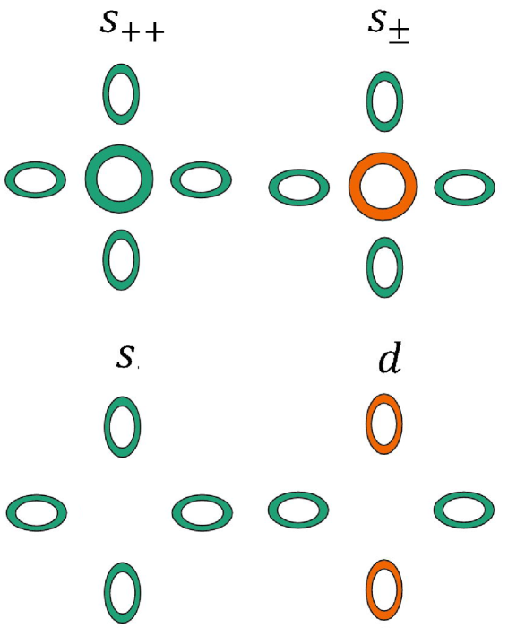
Figure 14: Main type of pairing in multiple – band scheme for superconductivity in FeAs and FeSe systems. Different colors represent different signs of superconducting gaps.

In second case we have $\Delta_{3}=\Delta_{4}$ and $\nu_{3}=\nu_{4}$, so that two equations in (6) just coincide and instead of (4), (7) appears the coupling matrix $3\times 3$ of the following form:

$$-\hat{g}=\left(\begin{array}[]{ccc}u\nu_{1}&w\nu_{2}&2t\nu_{3}\\ w\nu_{1}&u^{\prime}\nu_{2}&2t^{\prime}\nu_{3}\\ t\nu_{1}&t^{\prime}\nu_{2}&2\bar{\lambda}\nu_{3}\end{array}\right),$$ (10)

where $\bar{\lambda}=\frac{\lambda+\mu}{2}$ and solution of system of Eqs. (6) reduces to the standard procedure of finding the eigenvalues (and eigenvectors) for the matrix of dimensionless coupling constants $g_{ij}$ (10), which are determined by the cubic secular equation:

$$Det(g_{ij}-g_{eff}\delta_{ij})=0$$ (11)

Physical solution is determined by the maximal positive value of $g_{eff}$, which gives the maximal value of $T_{c}$. Eigenvectors of the problem determine here the ratios of the gaps $\Delta_{i}$ on different sheets of the Fermi surface for $T\to T_{c}$. Temperature dependencies of gaps for $T<T_{c}$ can be found by solving the system of generalized BCS equations:

$$\Delta_{i}=\sum_{j}g_{ij}\Delta_{j}\int_{0}^{\omega_{c}}d\xi\frac{th\frac{\sqrt{\xi^{2}+\Delta_{j}^{2}}}{2T}}{\sqrt{\xi^{2}+\Delta_{j}^{2}}}.$$ (12)

For $T\to 0$ these equations reduce to:

$$\Delta_{i}=\sum_{j}g_{ij}\Delta_{j}F\left(\frac{\Delta_{j}}{\omega_{c}}\right),\ F(x)=ln\left(\frac{1+\sqrt{1+x^{2}}}{|x|}\right)$$ (13)

This analysis makes it clear that the value of $T_{c}$ (effective pairing constant) in multiple bands system is determined, in general case, not only by the value of the total density of states at the Fermi level (multiplied by the single dimensional coupling constant), but by rather complicated combination of several coupling constants, multiplied by partial densities of states for different bands. Now it becomes obvious that the multiple – band structure of the spectrum can lead to the growth of $T_{c}$ by itself, reasonably enhancing the effective pairing constant in Eq. (5) KucSad08 . To understand the essence of this effect it is useful to analyze simple limiting cases.

Let the matrix of dimensionless coupling constants be diagonal (i.e. there are only intraband pairing interactions):

$$\hat{g}=\left(\begin{array}[]{cccc}g_{1}&0&0&0\\ 0&g_{2}&0&0\\ 0&0&g_{3}&0\\ 0&0&0&g_{3}\end{array}\right).$$ (14)

Then obviously $g_{eff}=Max\{{g_{i}}\}$ and $T_{c}$ is determined by the density of states and pairing interaction of the single (and in this sense dominating) pocket of the Fermi surface.

Let us consider in some sense opposite case, when all intraband and interband interactions in (4) are the same and also all partial densities of states are just equal. Then we can introduce $g_{0}=-u\nu$ and the matrix of dimensionless pairing constants takes the following form:

$$\hat{g}=g_{0}\left(\begin{array}[]{cccc}1&1&1&1\\ 1&1&1&1\\ 1&1&1&1\\ 1&1&1&1\end{array}\right).$$ (15)

In this case we obtain $g_{eff}=4g_{0}$, i.e. the real quadrupling of the effective pairing coupling constant, as compared to the single – band model (or the model without interband pairing couplings). The generalization for the case of $n\times n$ matrices is obvious.

In Refs. KucSad08 ; KucSad10 it was shown that a certain choice of coupling constants in this model (with the account of LDA calculated values of partial densities of states) allows, in principle rather easily, to explain the observed (by ARPES) values of gap ratios on different pockets of the Fermi surface for a number of FeAs based superconductors.

In Ref. Hirshf the similar analysis was done for a number of typical situations of electronic spectrum evolution, which can be realized in FeAs and FeSe based systems. It was explicitly shown that e.g. in the case of hole – like band approaching from below in energy (at the $\Gamma$ point) and crossing the Fermi level (Lifshits transition) $T_{c}$ and the values of energy gaps on hole – like and electron – like pockets of the Fermi surface actually grow. In Fig. 15 we show the results of calculations of Ref. Hirshf for one of the typical cases, which may be realized in systems under consideration. We can see that as the distance of hole – like band from the Fermi level $E_{g}$ diminish and change its sign (at Lifshits transition) there is a significant growth of $T_{c}$ and the gap values $\Delta_{i}$ (at $T$=0). Specific values of parameters used in this calculations can be found in Ref. Hirshf .

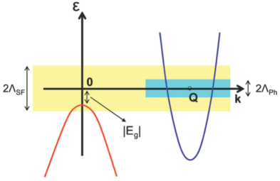
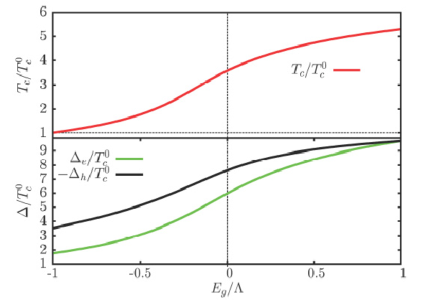
Figure 15: (a) – typical band structure of FeAs and FeSe based superconductors with hole – like band approaching to the Fermi level from below, crossed areas denote the energy regions around the Fermi level, where two pairing interactions operate, e.g. electron – phonon ($\Lambda_{ph}$) and spin – fluctuation ($\Lambda_{sf}$). (b) – $T_{c}$ and energy gaps (at $T=0$ and on different sheets of the Fermi surface) behavior during the crossing of the Fermi – level by hole – like band. $T_{c0}$ is the temperature of superconducting transition in the absence of hole – like band. All energies are in units of $\Lambda_{sf}$ Hirshf .

The basic conclusion from this elementary analysis is that the multiple – band structure, in general, facilitates the growth of effective pairing coupling constant and the growth of $T_{c}$. It is also clear that the opening of new pockets of the Fermi surface (during the Lifshits transition) also leads to the growth of $T_{c}$, while closing of such pockets leads to the drop of $T_{c}$. A number of experiments on FeAs systems under strong enough electron or hole doping evidently confirm these conclusions dop_1 ; dop_2 .

At the same time, the general picture of electron spectrum evolution during the transition from typical FeAs systems to intercalated FeSe systems, as well as all the data obtained for single – layer FeSe/STO, are in drastic contradiction with this conclusion — the high values of $T_{c}$ are achieved in these systems after the disappearance of hole – like pockets around the $\Gamma$ point and only electron – like pockets remain around $M$ points.

The energy gaps, appearing on these pockets are reliably measured in ARPES experiments and are practically isotropic FeSe_BTO ; ARP_FS_FeSe_2 . The relevant experimental data are shown in Fig. 16.

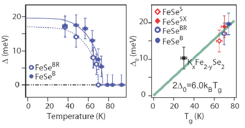
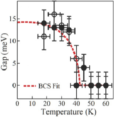
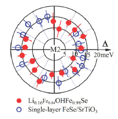
Figure 16: (a) – temperature dependence of energy gap for two FeSe/BTO films FeSe_BTO , (b) – the value of the gap for K_xFe_2-ySe₂ and monolayers of FeSe FeSe_BTO , (c) – temperature dependence of the energy gaps in Li_0.16Fe_0.84OHFe_0.98Se ARP_FS_FeSe_2 , (d) – angular dependence of energy gap in Li_0.16Fe_0.84OHFe_0.98Se and monolayer FeSe/STO ARP_FS_FeSe_2 .

These data give rather convincing evidence of either $d$-wave pairing (case 1 above) or the usual $s$-wave pairing in systems under discussion. Pairing of $s^{\pm}$-type can not be realized in these systems due to the absence (or smallness) of Fermi surface pockets around the $\Gamma$ point. The absence of “nesting” of electron – like and hole – like pockets of the Fermi surface also indicates the absence of well developed spin fluctuations, which can be responsible for repulsive interaction, leading to the picture of $s^{\pm}$ pairing.

Apparently, the most probable in these systems is the scenario of $s$-wave pairing, when the usual isotropic gap opens on electronic pockets. The variant of $d$-wave pairing (as in case 1) seems less probable. First of all, no microscopic mechanism (like spin fluctuations) was ever proposed for realization of repulsive interaction on characteristic inverse lattice vectors connecting electronic pockets at points $M$ (or $X$ and $Y$ points in Brillouin zone of Fig. 5 (b)). This picture also contradicts direct experiments on the influence of magnetic and non – magnetic adatoms on superconductivity in single – layer FeSe/STO films. It was shown in Ref. mag_imp , that magnetic adatoms suppress superconductivity, while non – magnetic adatom practically do not influence it at all. This obviously corresponds to the picture of $s$-wave pairing.

IV.3 Models of $T_{c}$ enhancement in FeSe monolayer due to interaction with elementary excitations in the substrate

From the previous discussion it is clear that the values of $T_{c}\sim$40 K in intercalated FeSe layers can be achieved, in principle, by increasing the density of states at the Fermi level, as compared with its value for bulk FeSe, which may be connected with the evolution of the band structure and doping. At the same time, it is also clear that the enhancement of $T_{c}$ up to the values exceeding 65 K, observed in FeSe monolayers on STO(BTO), can not be explained along these lines. It is natural to assume that this enhancement is somehow related to the nature of STO(BTO) substrate, e.g. with additional pairing interaction of carriers in FeSe layer, appearing due to their interaction with some kind of elementary excitations in the substrate, in the spirit of “excitonic” mechanism, as was initially proposed by Ginzburg VLG ; HTSC77 .

It is well known that SrTiO₃ is a semiconductor with indirect gap equal to 3.25 eV STO_el_str . At room temperature it is paraelectric with very high dielectric constant, reaching the values of $\sim$10⁴ at low temperatures, remaining in paraelectric state STO_parael . It is interesting to note that under electron doping, in concentration interval from 6.9 10¹⁸cm^-3 to 5.5 10²⁰cm^-3 SrTiO₃ becomes superconductor with maximal value of $T_{c}\sim$0.25K at electronic concentration of the order of 9 10¹⁹cm^-3 KCSHP ; XLin . The origin of superconductivity at such low concentrations (and general form of corresponding phase diagram) is by itself the interesting separate problem.

IV.3.1 Excitonic mechanism of Allender, Bray and Bardeen

The structure of FeSe films on SrTiO₃, shown Fig. 3, represents the typical Ginzburg’s “sandwich” VLG , which indicates the possibility of realization of excitonic mechanism of superconductivity. Let us consider the widely known version of this mechanism, as proposed for such a system long ago by Allender, Bray and Bardeen (ABB) ABB . Schematically this mechanism is shown in Fig. 17. Electron from metal with momentum ${\bf k}_{1\uparrow}$ (arrow denotes spin direction) is transferred into the state ${\bf k}_{2\uparrow}$, due to excitation of interband transition in semiconductor from valence band state ${\bf k}_{v}$ into ${\bf k}_{c}$ state in conduction band, creating the virtual exciton. The second electron of Cooper pair, which is initially in $-{\bf k}_{1\downarrow}$ state, absorbs this exciton and goes into $-{\bf k}_{2\downarrow}$ state. The momentum conservation law holds: ${\bf q}={\bf k}_{2}-{\bf k}_{1}={\bf k}_{v}-{\bf k}_{c}+{\bf K}$, where K is an arbitrary inverse lattice vector. As a result we obtain electron attraction within the pair, which is conceptually identical to that appearing due to phonon exchange.

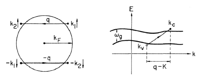
Figure 17: ABB excitonic mechanism.

In Ref. ABB a rough estimate of the corresponding attraction coupling constant was obtained as:

$$\lambda_{ex}=ba\mu\frac{\omega_{p}^{2}}{\omega_{g}^{2}}$$ (16)

where $\mu$ is the dimensionless Coulomb potential, $\omega_{p}$ – the plasma frequency in semiconductor, while $\omega_{g}$ is the width of the energy gap in semiconductor, which plays the role of exciton energy. Dimensionless constant $b\sim$ 0.2 defines the fraction of time the metallic electron spends inside the semiconductor, and the constant $a\sim$ 0.2-0.3 is related to screening of Coulomb interaction within metal. This estimate was criticized in Refs. IA_73 ; UspZhar as an overestimate, additional arguments in favor of it were given in Ref. ABB_2 . Without returning to this discussion, we further use the estimate of Eq. (16) as obviously too optimistic.

To estimate $T_{c}$ due to two mechanisms of attraction (phonon and exciton) Ref. ABB proposed to use the following simple expression, which gives (as was shown in ABB ) a good approximation to numerical solution of appropriate Eliashberg equations:

$$T_{c}=\frac{\omega_{D}}{1.45}\exp\left(-\frac{1}{g_{eff}}\right),$$ (17)

where

$$g_{eff}=\lambda_{ph}^{\star}+\frac{\lambda_{ex}^{\star}-\mu^{\star}}{1-(\lambda_{ex}^{\star}-\mu^{\star})\ln\left(\frac{\omega_{g}}{\omega_{D}}\right)}$$ (18)

$$\mu^{\star}=\frac{1}{1+\mu\ln\left(\frac{E_{F}}{\omega_{g}}\right)}$$ (19)

and the constants of electron – phonon and exciton attraction are taken here in renormalized form:

$$\lambda_{ph}^{\star}=\frac{\lambda_{ph}}{1+\lambda_{ph}},\ \lambda_{ex}^{\star}=\frac{\lambda_{ex}}{1+\lambda_{ex}},\$$ (20)

which takes into account qualitatively the effects of strong coupling. $E_{F}$ is the Fermi energy of metallic film.

Is we consider $\lambda_{ex}$ a free parameter, we can easily estimate the possible extent of $T_{c}$ enhancement due to excitonic mechanism. Corresponding dependencies, calculated from Eqs. (17),(18),(19), (20) for typical values of Coulomb potential $\mu$, are shown Fig. 18 (a). The value of $\omega_{D}$ was taken to be 350 K, while $\lambda_{ph}=$ 0.437, to reproduce the value of $T_{c}=$ 9 K, typical for bulk FeSe, while $E_{F}=$ 0.2 eV was taken to be in agreement with LDA calculations of FeSe monolayer. From Fig. 18 (a) we can see that for large enough values of $\lambda_{ex}$ very high values of $T_{c}$ can be easily obtained (as it was predicted in Ref. ABB ).

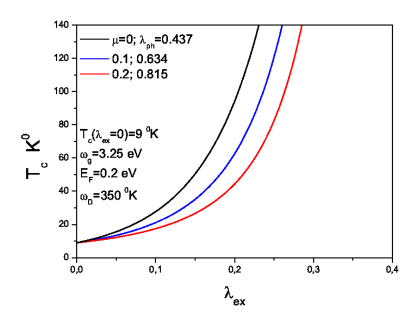
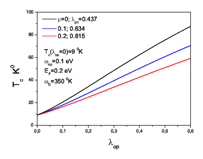
Figure 18: Dependence of $T_{c}$ for FeSe/STO on coupling constant with ABB exciton (a) and optical phonon in STO (b).

The problem, however, is that even using the very optimistic estimate of $\lambda_{ex}$ in Eq. (16), taking characteristic values of $\omega_{p}=$ 10 eV, $\omega_{g}=$ 3.25 eV, for typical $\mu\sim$ 0.1-0.2, we obtain the values of $\lambda_{ex}\sim$ 0.04-0.13. Correspondingly, as we can see from Fig. 18 (a), even for these over optimistic estimates, we obtain quite modest enhancement of $T_{c}$ and it is very far from the desirable values of $\sim$ 65-75 K. These estimates convincingly demonstrate ineffectiveness of ABB excitonic mechanism in FeSe/STO monolayers.

IV.3.2 Interaction with optical phonons in STO

The initial Ginzburg’s guess to enhance $T_{c}$ in “sandwich” type structures VLG was based on the idea of electron in metallic film interaction with more or less high – energy excitations of electronic nature (“excitons”) within semiconducting substrate. However, this idea can be understood in a wider context — interaction of electrons of metallic film with some arbitrary Boson excitations in substrate (e.g. with phonons) can lead to the enhancement of $T_{c}$. As we shall see, precisely this scenario is probably realized in FeSe monolayers on STO(BTO). The thing is that in SrTiO₃ or BaTiO₃ like systems almost dispersionless optical phonons exist with unusually high excitation energy of the order of $\sim$ 100 meV CWK . Examples of phonon dispersions and densities of states in these systems (both calculated and measured by neutron scattering) are shown in Fig. 19.

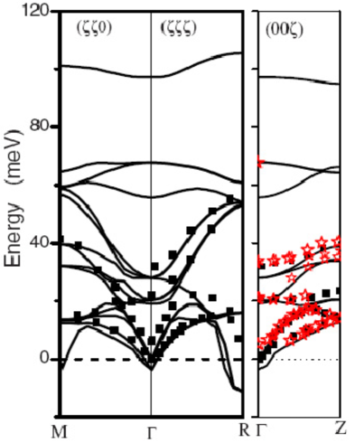
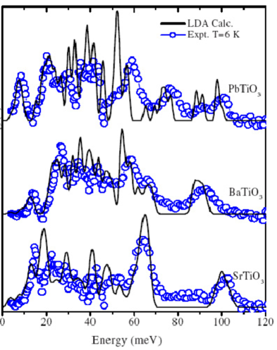
Figure 19: Phonons in SrTiO₃ and similar compounds: (a) — phonon dispersions in SrTiO₃, both calculated and measured by inelastic neutron scattering, (b) — phonon density of states in SrTiO₃, BaTiO₃ SrTiO₃ from neutron scattering and calculations CWK .

To estimate the prospects of $T_{c}$ enhancement due to interaction with such phonons we can again use the expressions (17),(18), (19),(20), with simple replacements of $\omega_{g}\to\omega_{op}$ and $\lambda_{ex}\to\lambda_{op}$, where $\omega_{op}$ is characteristic frequency of optical phonon, $\lambda_{op}$ is dimensionless coupling constant for such phonon with electrons within metallic film. Results of such calculations of $T_{c}$ versus $\lambda_{op}$ (similar to those shown in Fig. 18 (a) for ABB excitonic mechanism) with the choice of $\omega_{op}=$ 0.1 eV are shown in Fig. 18 (b). It can be seen that for large enough values of $\lambda_{op}\sim$ 0.5-0.6 and not very large $\mu$ we can easily achieve values of $T_{c}\sim$ 60-80 K, corresponding to experiments on FeSe/STO(BTO), even if we start from relatively low initial $T_{c}\sim$ 9 K for FeSe in the absence of additional pairing interaction. Corresponding values of $\lambda_{op}$ seem to be realistic enough and below we shall present concrete evidence that interaction with optical phonons in these structures can be strong enough.

The idea that interaction with optical phonons in STO can play a significant role in physics of FeSe/STO monolayers was first proposed in Ref. ARPES_FeSe_Nature in connection with ARPES measurements done in this work, which demonstrated the formation of a “shadow” band at the $M$ point in Brillouin zone, as shown in Fig. 11 (b). This band is situated approximately 100 meV below the main conduction electronic band and practically replicates its dispersion. Formation of such band can be linked with interaction of FeSe electrons with optical phonon of appropriate energy in STO. To understand this situation we have to consider a realistic enough picture of FeSe monolayer electrons interacting with optical phonons in STO, which was proposed in Refs. ARPES_FeSe_Nature and will be briefly described below (cf. also DHL ).

As STO is in almost ferroelectric state it is natural to expect that charge transfer at the interface can induce the appearance of the layer of ordered dipoles. Free carriers in STO, appearing for example due to oxygen vacancies (or Nb doping) will screen the electric field far from the interface. Then, the dipole layer will be localized close to the interface. The appearance of dipoles is connected with the displacement of Ti cations relative to oxygen anions, so that oscillations of these anions will lead to modulation of dipole potential along the FeSe layer. Schematically, this situation is shown in Fig. 20 (a).

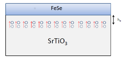
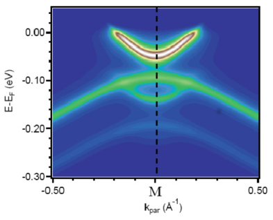
Figure 20: (a) – schematic picture of dipole excitations close to FeSe/STO interface , (b) – calculated electron spectral density in FeSe/STO in the model with dominating forward scattering ARPES_FeSe_Nature .

Let $\delta P_{z}$ denote the change of dipole moment due to displacement of oxygen anions in the direction perpendicular to interface:

$$\delta P_{z}(x,y,-h_{0})=q_{eff}\delta h(x,y,-h_{0}).$$ (21)

Here $x,y$ are coordinates in the plane parallel to interface and the origin of $z$ - axis is chosen in Fe plane, $q_{eff}$ is dipole charge. With respect to Fe plane the dipole layer is at $z=-h_{0}$. The induced change of dipole potential in Fe plane connected with the “frozen” displacement of oxygens is given by the following expression:

$$\Phi(x,y,0)=\frac{{\epsilon}_{\parallel}^{1/2}q_{eff}h_{0}}{\epsilon_{\perp}^{3/2}}n_{d}\int dx^{\prime}dy^{\prime}\frac{\delta h(x^{\prime},y^{\prime},-h_{0})}{\left(\frac{\epsilon_{\parallel}}{\epsilon_{\perp}}h_{0}^{2}+(x-x^{\prime})^{2}+(y-y^{\prime})^{2}\right)^{3/2}}.$$ (22)

Performing Fourier transformation over $x,y$, we get:

$$\Phi({\bf q}_{\parallel},0)=\frac{2\pi q_{eff}n_{d}}{\epsilon_{\perp}}\exp\left({-|{\bf q}_{\parallel}|h_{0}\sqrt{\epsilon_{\parallel}/\epsilon_{\perp}}}\right)\delta h({\bf q}_{\parallel},-h_{0}).$$ (23)

Here ${\bf q}_{\parallel}$ is the wave-vector parallel to the interface and $\epsilon_{\parallel},\epsilon_{\perp}$ are dielectric constants parallel and perpendicular to the interface, $n_{d}$ is density of dipole per unit square of the interface. As electrons in FeSe move parallel to interface, they contribute only to $\epsilon_{\parallel}$. As to carriers in STO, besides their role in screening which we have mentioned above, they give approximately equal contributions (STO has cubic structure) both to $\epsilon_{\parallel}$ and $\epsilon_{\perp}$. Thus, we can expect that the total dielectric constant $\epsilon_{\parallel}$ is much greater than $\epsilon_{\perp}$.

From Eq. (23) it becomes clear that the value of the matrix element of electron – phonon interaction has an important dependence on ${\bf q}_{\parallel}$, so that it can be written as:

$$\Gamma(p_{\parallel},q_{\parallel})=\frac{2\pi q_{eff}n_{d}}{\epsilon_{\perp}}\exp\left({-|{\bf q}_{\parallel}|/q_{0}}\right),$$ (24)

$$q_{0}^{-1}=h_{0}\sqrt{\epsilon_{\parallel}/\epsilon_{\perp}}.$$ (25)

The fact that $\epsilon_{\parallel}\gg\epsilon_{\perp}$ leads to $q_{0}$ suppression by the factor of $1/\sqrt{\epsilon_{\parallel}/\epsilon_{\perp}}$, which in turn leads to a sharp enough peak in electron – phonon interaction at ${\bf q}_{\parallel}=0$. Such dominating role of forward scattering explains the appearance of the “shadow” band in electronic spectrum, which replicates the dispersion of the main band. In the case of electron – phonon interaction acting in the wide range of transferred momenta, it will lead to a superposition of many bands, each being moved by its own scattering vector, which will lead to a general smearing of the “shadow” band.

The standard numerical calculation of second – order electron self – energy due to electron – phonon interaction was performed in Ref. ARPES_FeSe_Nature with coupling constant written as $g({\bf q})=g_{0}\exp(-|{\bf q}|/q_{0})$, with $g_{0}=$ 0.04 eV, $q_{0}=0.3/a$ (a=3.9Å), optical phonon frequency $\Omega_{0}=$ 80 meV, and the bare spectrum of electrons and holes (one-dimensional — along $\Gamma-M$ direction) close to the $M$ point written as $\epsilon_{e,h}(k)=-2t_{e.h}\cos(k/a)-\mu_{e,h}$ with $t_{e}=$ 125 meV, $t_{h}=$ 30 meV, $\mu_{e}=$ - 185 meV and $\mu_{h}=$ 175 meV, where all numerical parameters were taken from fitting the ARPES experiment. Results of such calculation for electron spectral density (imaginary part of Green’s function) are shown in Fig. 20 (b). We can see that these calculations are in excellent agreement with ARPES data of Fig. 11 (b). The standard dimensionless electron – phonon coupling constant can be estimated numerically using the same values of all parameters giving ($N$ is the number of lattice sites) ARPES_FeSe_Nature :

$$\lambda=\frac{2}{N\Omega_{0}}\frac{\sum_{{\bf k},{\bf q}}|g({\bf q})|^{2}\delta{(\epsilon_{e}{(\bf k)})}\delta(\epsilon_{e}{(\bf k-q)})}{\sum_{\bf k}\delta(\epsilon_{e}({\bf k}))}=0.5$$ (26)

which is (as noted above) quite sufficient for significant enhancement of $T_{c}$ in FeSe/STO monolayer. As we shall see below, the peculiarities of the model of electron – phonon interaction with dominating forward scattering lead also to some other, even more important, effects enhancing $T_{c}$.

IV.3.3 Cooper pairing in the model with dominating forward scattering

Dominating forward scattering in electron – phonon interaction was for a long time considered as a special cause for $T_{c}$ enhancement due to specific dependencies differing from the standard BCS, which appear in this model DaDoKuO ; Kulic . These papers analyzed the possible role of such interactions in cuprates. An application of these ideas to FeSe/STO was considered recently in Rade_1 ; Rade_2 .

In weak coupling approximation, for the case of $s$-wave pairing, the gap equation in Eliashberg theory reduces to ($\varepsilon_{n}=(2n+1)\pi T$ – is Fermion Matsubara frequency):

$$\Delta(i\varepsilon_{n}) = -\frac{T}{N}\sum_{{\bf q},m}|g({\bf q})|^{2}D({\bf q},i\varepsilon_{n}-i\varepsilon_{m})\frac{\Delta(i\varepsilon_{m})}{(\varepsilon_{m})^{2}+\xi_{{\bf k}+{\bf q}}^{2}+\Delta^{2}(i\varepsilon_{m})}.$$ (27)

where $D({\bf q},i\varepsilon_{n}-i\varepsilon_{m})=-\frac{2\Omega_{\bf q}}{(\varepsilon_{n}-\varepsilon_{m})^{2}+\Omega_{\bf q}^{2}}$ is Matsubara Green’s function of an optical phonon with frequency $\Omega_{\bf q}$, $\xi_{\bf k}=v_{F}(|{\bf k}|-p_{F})$ is the electronic spectrum close to the Fermi level ($v_{F}$, $p_{F}$ are Fermi velocity and momentum).

Before going to the results of numerical solution of this equation, let us consider the elementary model of exactly forward scattering by phonons, when all calculations can be done analytically. For this purpose we introduce $|g({\bf q})|^{2}=g^{2}_{0}N\delta_{\bf q}=(2\pi)^{2}\delta({\bf q})$. Then the gap equation (27) at the Fermi surface is easily transformed to:

$$\Delta(i\varepsilon_{n})=\lambda_{m}\Omega^{2}_{0}T_{c}\sum_{m}\frac{\Delta(i\varepsilon_{m})}{\varepsilon_{m}^{2}+\Delta^{2}(i\varepsilon_{m})}\frac{2\Omega_{0}}{\Omega^{2}_{0}+(\varepsilon_{n}-\varepsilon_{m})^{2}},$$ (28)

where we have introduced the dimensionless coupling constant

$$\lambda_{m}=g^{2}_{0}/\Omega^{2}_{0}.$$ (29)

Note that this definition is somehow different from the standard definition of electron – phonon coupling constant (26).

To find the critical temperature $T_{c}$ the authors of Ref. Rade_1 used the following Ansatz for the gap function:

$$\Delta(i\varepsilon_{n})=\Delta_{0}/[1+(\varepsilon_{n}/\Omega_{0})^{2}]$$ (30)

Then, linearizing the gap equation we can obtain the following equation for $T_{c}$ Rade_1 :

$$1=\lambda_{m}\Omega^{2}_{0}T_{c}\sum_{m}\frac{2\Omega_{0}}{\varepsilon^{2}_{m}(1+\varepsilon^{2}_{m}/\Omega^{2}_{0})(\Omega^{2}_{0}+\varepsilon_{m}^{2})}.$$ (31)

The sum over Matsubara frequencies is calculated directly and we obtain:

$$1=\frac{\lambda_{m}}{2T_{c}}\frac{2\Omega_{0}+\Omega_{0}\cosh(\Omega_{0}/T_{c})-(3T_{c})\sinh(\Omega_{0}/T_{c})}{1+\cosh(\Omega_{0}/T_{c})}.$$ (32)

For FeSe/STO $T_{c}\ll\Omega_{0}$, so that we can use the asymptotics of hyperbolic functions and in the leading approximation the critical temperature becomes the quasi – linear function of the coupling constant (for its small values):

$$T_{c}=\frac{\lambda_{m}}{2+3\lambda_{m}}\Omega_{0}.$$ (33)

Similar result was previously obtained in the context of cuprates physics DaDoKuO ; Kulic . For $\lambda_{m}=$ 0.16 and $\Omega_{0}=$ 100 meV we get $T_{c}=75$ K, which is rather unexpected for such a small value of $\lambda_{m}$.

This value of $T_{c}$ can be compared with the standard expression of BCS theory where the linearized equation for $T_{c}$ takes the following form:

$$1=\pi T_{c}\lambda_{m}\sum_{|\varepsilon_{m}|<\omega_{D}}\frac{1}{|\varepsilon_{m}|}=\lambda_{m}\left[\ln\left(\frac{\omega_{D}}{2\pi T_{c}}\right)-\psi\left(\frac{1}{2}\right)\right],$$ (34)

where we have used the asymptotics of large $\omega_{D}/T_{c}$. This leads to the usual BCS expression: $T_{c}=1.13\omega_{D}\exp(-1/\lambda_{m})$, so that for $\lambda_{m}=0.16$ and $\omega_{D}=$ 100 meV we obtain $T_{c}=$ 2.5K.

Comparing these results for $T_{c}$ we can conclude that the significant $T_{c}$ enhancement obtained above appears due to effective exclusion of momentum integration in Eliashberg equation, which is related to the strong interaction peak at ${\bf q}=0$. In BCS model we integrate over the whole of the Fermi surface and all momenta enter with the same weight, which leads to the appearance of $\sum_{m}1/|\varepsilon_{m}|$ term in the equation for $T_{c}$ and corresponding logarithmic behavior. In the case of forward scattering integration over momenta is lifted, so that in the sum over frequencies only the $\varepsilon_{m}^{-2}$ term remains, which leads to $1/T_{c}$ behavior. Due to this the model with strong forward scattering leads to the effective mechanism of $T_{c}$ enhancement DaDoKuO ; Kulic .

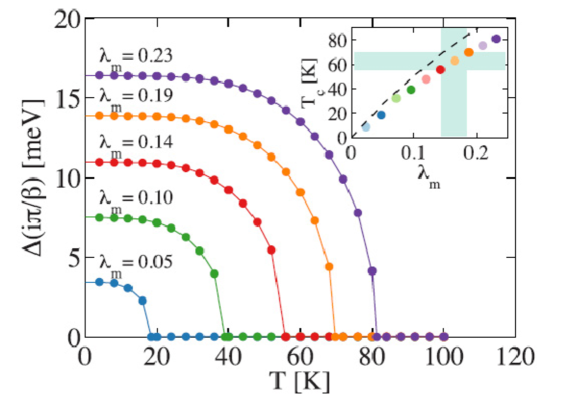
Figure 21: Temperature dependence of the energy gap $\Delta(i\pi T)$ (at the smallest Matsubara frequency) in the model with dominating forward scattering ($q_{0}=0.1/a$) for different values of the coupling constant. At the insert the dashed line shows $T_{c}$ coupling constant dependence in the case of exactly forward scattering (33), while the dots represent the results of numerical calculation Rade_1 . The dashed region show the interval of $\lambda_{m}$ values appropriate for FeSe/STO.

Let us now discuss the numerical results for the general case Rade_1 . In realistic situation, the forward scattering dominates in the finite region of momentum space, with the size determined by the parameter $q_{0}$. Numerical solution of Eliashberg equations with the coupling constant of the form $g({\bf q})=g_{0}\exp(-|{\bf q}|/q_{0})$, gives the temperature behavior of the superconducting gap (at the lowest Matsubara frequency) $\Delta(i\pi T)$ shown in Fig. 21 (for several values of $\lambda_{m}$ and $q_{0}=0.1/a$). We can see that $T_{c}$ is high enough already for modest enough values of $\lambda_{m}$ and grows approximately linearly over $\lambda_{m}$, while we remain in the weak coupling region. The finiteness of $q_{0}$ leads to some suppression of $T_{c}$ as compared with the case of exact forward scattering (cf. the insert in Fig. 21), but in general case the quasi – linear dependence of $T_{c}$ on $\lambda_{m}$ can guarantee the values of $T_{c}$ observed in FeSe/STO films.

In the framework of this model it is rather easy to explain the formation of the “shadow” band in the vicinity of the $M$ point Rade_1 ; Rade_2 .

IV.3.4 Nonadiabatic superconductivity and other problems

We have already noted above, that the characteristic feature of electronic spectrum of superconductors containing FeSe monolayers is the formation of unusually “shallow” electronic band in the vicinity of $M$ point in Brillouin zone (cf. Fig. 9 (d), 11 (b)). The value of Fermi energy $E_{F}\sim$ 0.05 eV in these systems is almost an order of magnitude less than the values obtained in LDA and LDA+DMFT calculations. Such small value of $E_{F}$ creates additional difficulties for consistent theory of superconductivity in FeSe/STO system. Gor’kov was the first to note Gork_1 that here we are dealing with an unusual situation, when the energy of an optical phonon in STO $\sim$ 100 meV is significantly larger than Fermi energy $\sim$ 50 meV. Let us remind that in the great majority of superconductors we have the opposite inequality $\omega_{D}\ll E_{F}$, which allows us to use the adiabatic approximation to describe the effects of electron – phonon interaction, which is based upon the inequality $\frac{\omega_{D}}{E_{F}}\sim\sqrt{\frac{m}{M}}\ll 1$ ($m$ is electron mass, $M$ is an ion mass). Then (as in the normal state) we can apply Migdal theorem and neglect all vertex corrections in electron – phonon interaction, limiting ourselves to second – order diagrams for electron self – energy. In particular, the standard derivation of Eliashberg equations is entirely based on adiabatic approximation, so that the common term is “Migdal – Eliashberg theory”. Breaking the relevant inequality in FeSe/STO means that the theory explaining $T_{c}$ enhancement is to be developed, from the very beginning, in the antiadiabatic approximation. An attempt to build such a theory was undertaken in recent papers by Gor’kov Gork_1 ; Gork_2 ; Gork_3 . In particular, Refs. Gork_1 ; Gork_2 were devoted to FeSe/STO system and the general aspects of the problem, while in Ref. Gork_3 a new theory was proposed for superconductivity in doped SrTiO₃, which, as was noted above, is by itself quite unusual superconductor KCSHP ; XLin .

Obviously, the nature of our review does not allow us to go deeply inside the discussion of rather complicated theoretical problems, so that we shall limit ourselves only to qualitative presentation of the results of Refs. Gork_1 ; Gork_2 , which are directly relevant to superconductivity in FeSe/STO. The only approximation, which can be apparently used here is the weak coupling approximation, when the smallness of electron – phonon coupling constant by itself allows to sum the usual (ladder) series of Feynman diagrams in Cooper channel. It is natural that in antiadiabatic approximation the cut-off of logarithmic divergence in Cooper channel takes place not on phonon frequencies, but at energies of the order of Fermi energy $E_{F}$ (or the bandwidth) Gork_2 , so that we can expect $T_{c}\sim E_{F}\exp(-1/\lambda)$, where $\lambda$ is determined by the details of pairing interaction.

The interaction of FeSe electrons with longitudinal surface phonons at the STO interface can be introduced Gork_1 via interactions with polarization induced by these phonons:

$${\bf P}=F_{C}{\bf u},$$ (35)

where ${\bf u}$ is atomic displacement and coefficient $F_{C}$ is determined by the model of electron interaction with optical surface (SLO) phonons at the surface of an insulator Mahan :

$$F_{C,i}=\left[4\pi e^{2}\frac{\omega^{i}_{SLO}}{2}\left(\frac{1}{\epsilon_{\infty}+1}-\frac{1}{\epsilon_{0}}\right)\right]^{1/2}$$ (36)

where $i$ enumerates phonon branches, while $\epsilon_{0}$ and $\epsilon_{\infty}$ are static and optical dielectric constants of the bulk insulator, and $\omega^{i}_{SLO}$ is the frequency of $i$-th SLO phonon.

Then the matrix element for two – electron scattering due to exchange of surface phonon takes the form:

$$M_{i}({\bf q},\varepsilon_{n}-\varepsilon_{m})=-\frac{4\pi e^{2}}{|{\bf q}|}\left(\frac{1}{\epsilon_{\infty}+1}-\frac{1}{\epsilon_{0}}\right)D^{i}_{SLO}({\bf q},\varepsilon_{n}-\varepsilon_{m})$$ (37)

where $D^{i}_{SLO}({\bf q})$ is Green’s function of STO phonon:

$$D^{i}_{SLO}({\bf q},\varepsilon_{n}-\varepsilon_{m})=\frac{(\omega^{i}_{SLO})^{2}}{(\omega^{i}_{SLO})^{2}+(\varepsilon_{n}-\varepsilon_{m})^{2}},$$ (38)

where ${\bf q}={\bf p}-{\bf k}$ and $\varepsilon_{n}-\varepsilon_{m}$ are momentum and (Matsubara) frequency exchanged between electrons.

In the bulk insulator the well known Lyddane – Sachs – Teller relation holds between the frequencies of longitudinal (LO) and transverse (TO) optical phonons: $\omega^{2}_{LO}/\omega^{2}_{TO}=\epsilon_{0}/\epsilon_{\infty}$. According to Ref. Mahan , the frequency of longitudinal surface phonon is given by the following expression: $\omega^{2}_{SLO}/\omega^{2}_{TO}=\epsilon_{0}+1/\epsilon_{\infty}+1$. It should be stressed that the values of $\epsilon_{0}$ and $\epsilon_{\infty}$ are considered here as model parameters, depending on the details of STO surface preparation in the process of creation of FeSe/STO structures Gork_1 (e.g. SrTiO₃ doping by Nb) Gork_1 .

Finally, for the matrix element of two – electron scattering due to the exchange of surface LO phonons and (two – dimensional) Coulomb repulsion, dropping some irrelevant at the moment factors Gork_1 , we obtain:

$$M_{tot}({\bf p},\varepsilon_{n}|{\bf k},\varepsilon_{m})=\frac{4\pi e^{2}}{(\epsilon_{\infty}+1)q}-\sum_{i}\frac{4\pi e^{2}}{(\epsilon_{\infty}+1)q}D^{i}_{SLO}(\varepsilon_{n}-\varepsilon_{m})$$ (39)

Here the summation is performed over three IR – active phonons at $\Gamma$ point of the bulk SrTiO₃, with frequencies satisfying the inequality $\omega^{i}_{LO}>T_{c}$ CWK . In fact, in SrTiO₃ we have the single LO mode, which has a very large gap, as compared to the frequencies of all TO phonons, and which is of principal importance here compensating the Coulomb repulsion in Eq. (39) for $|\varepsilon_{n}-\varepsilon_{m}|\ll\omega_{LO}$. The remaining LO phonons, as usual, provide the additional contribution to attraction, As in SrTiO₃ we have $\epsilon_{0}\gg\epsilon_{\infty}$, in Eq. (39) we have left only the terms with $\epsilon_{\infty}+1$.

In extremely antiadiabatic limit, when $\omega_{SLO}\gg E_{F}$, we can neglect $(\varepsilon_{n}-\varepsilon_{m})^{2}$ terms in the denominator of phonon Green’s function, so that the matrix element of two – electron interaction can be written as:

$$M_{tot}({\bf p},\varepsilon_{n}|{\bf k},\varepsilon_{m})=M({\bf p}-{\bf k})\approx-2\alpha^{2}\frac{4\pi e^{2}}{|{\bf p}-{\bf k}|(\epsilon_{\infty}+1)}<0.$$ (40)

Here $\alpha^{2}<1$ are some numerical correction factors Gork_1 .

Now we also have to take into account the screening of Coulomb interaction by two – dimensional electron gas of FeSe. Then, in RPA approximation we get Gork_1 :

$$M_{scr}({\bf p}-{\bf k})\approx-2\alpha^{2}\frac{4\pi e^{2}}{\epsilon_{\infty}}\frac{1}{|{\bf p}-{\bf k}|+4e^{2}m/(\epsilon_{\infty}+1)}.$$ (41)

In experimental situation typical for FeSe/STO the inverse screening length $q_{0}$ is small as compared with Fermi momentum $p_{F}$, so that the following inequality always holds:

$$p_{F}/q_{0}=p_{F}(\epsilon_{\infty}+1)/e^{2}m\gg 1.$$ (42)

Introducing the effective Bohr radius $a_{B}=(\epsilon_{\infty}+1)/e^{2}m$ this inequality can be rewritten as $p_{F}a_{B}\gg 1$.

In weak coupling approximation the linearized gap equation can be written as Gork_1 :

$$\Delta({\bf p})=-T\sum_{m}\int\frac{d^{2}k}{(2\pi^{2})}M_{scr}({\bf p}-{\bf k})G(-{\bf k})G({\bf k})\Delta({\bf k}),$$ (43)

where the product of two Green’s functions $G(-{\bf k})G({\bf k})=[\varepsilon_{m}^{2}+\xi^{2}_{\bf k}]^{-1}$.

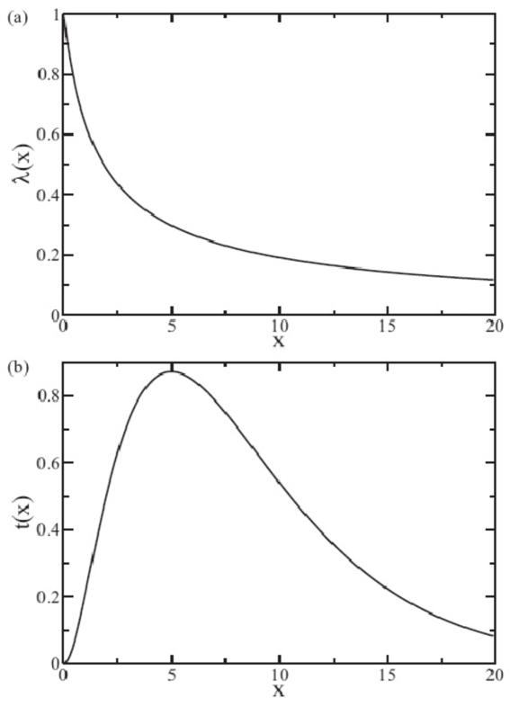
Figure 22: Dimensionless functions determining $T_{c}$ in Gor’kov’s model: (a) $\lambda(x)$ function, (b) $t(x)=x^{2}\exp[-1/\lambda(x)]$ function.

Then, after some a little bit cumbersome, though direct, analysis we can obtain the following result for the critical temperature $T_{c}$:

$$T_{c}(x)\sim\frac{p_{F}^{2}}{2m}\exp\left[-\frac{1}{\alpha^{2}\lambda(x)}\right]=$$

$$=\frac{2}{ma_{B}^{2}}x^{2}\exp\left[-\frac{1}{\alpha^{2}\lambda(x)}\right]$$ (44)

where we have introduced the dimensionless parameter $x=(p_{F}a_{B})/2$ and

$$\lambda(x)=\frac{2}{\pi}\int_{0}^{\pi/2}\frac{du}{x\sin u+1}.$$ (45)

For our estimates we can just put $\alpha^{2}=1$. Two dimensionless functions $\lambda(x)$ and $t(x)=x^{2}\exp[-1/\lambda(x)]$ are shown in Fig. 22. The maximum in $t(x)$ appears due to two competing factors: for the given value of $a_{B}$ the critical temperature first grows with growth of electron concentration and then the increased screening suppresses the effective coupling constant.

Direct calculations Gork_1 show, that this model also reproduces the “shadow” band in the electronic spectrum in the vicinity of $M$ point. This is essentially due to the fact, that from the form of pairing interaction (41) it becomes clear, that Gor’kov’s model produces the significant growth of interaction at small transferred momenta. Effective interaction is concentrated in momentum region inside the inverse screening length $q_{0}$, satisfying inequality (42), so that $q_{0}\ll 1/a$, in accordance with the estimates given above for the model with dominating forward scattering.

Let us make the simplest estimate of the maximal value of $T_{c}$, which can be achieved in this model. We take $E_{F}=$ 60 meV, which approximately corresponds to ARPES experiments. Maximum of $t(x)$ as can be seen from Fig. 22 (b) is close to $x=5$, which corresponds to $\lambda(5)=$ 0.3 (cf. Fig. 22(a)). Then we get $T_{c}\approx$ 0.03$\times$60 meV $\approx$ 20 K. Thus, this mechanism by itself can not explain the values of $T_{c}>$ 60 K, observed in experiments on FeSe/STO. However, in combination with some additional pairing mechanism, responsible for the initial value of $T_{c}\sim$ 8 K in bulk FeSe (either due to the usual electron – phonon mechanism or pairing due exchange of antiferromagnetic fluctuations) we can obtain significantly higher values of $T_{c}$ Gork_1 . For example, if for spin – fluctuation mechanism we use the estimate $T_{c}\sim E_{F}\exp(-1/\lambda_{sf})$, then for $E_{F}=$ 60 meV the initial value of $T_{c}$ is obtained for $\lambda_{sf}=0.23$. Then the combined pairing constant $\lambda=\lambda_{sf}+\lambda(5)=$ 0.48 (assuming the same cut-off in Cooper channel the coupling constants are just summed) leading to $T_{c}\approx$ 0.15$\times$60 meV$\approx$ 90 K. In the case of combination with the usual electron – phonon mechanism, we can estimate $T_{c}$ using the upper curve (corresponding to $\mu$=0) in Fig. 18 (b). Then, taking $\lambda_{op}=\lambda(5)=$ 0.3 we immediately obtain $T_{c}\approx$ 50 K.

The situation with nonadiabatic effects in the model with dominating forward scattering was recently analyzed in Ref. Rade_2 by direct calculations of vertex corrections to electron – phonon interaction with coupling constant $|g({\bf q})|^{2}=g_{0}^{2}N\delta_{\bf q}$. It was shown, that in this model Migdal theorem is invalid for any values of $\Omega_{0}/E_{F}$ ratio, which does not appear at all in vertex corrections. However, vertex corrections remain small for small values of the parameter $\lambda_{m}=g_{0}^{2}/\Omega_{0}^{2}$, and we have seen above, that to explain the current experiments on FeSe/STO it is sufficient to take the values $\lambda_{m}\sim$ 0.15-0.2.

The small values of Fermi energy $E_{F}$ in electron band at $M$ point, observed in intercalated FeSe systems and FeSe/STO(BTO), lead to one more important consequence. Typical values of superconducting gap at low temperatures, observed in ARPES measurements on these systems, are $\Delta\sim$ 15-20 meV (cf. Fig. 16). Correspondingly, here we have unusually large values of $\Delta/E_{F}\sim$ 0.25-0.3, which unambiguously show, that these systems belong to the region of BCS – Bose crossover NozSR ; Rand , when the size of Cooper pairs, determined by coherence length $\xi$, becomes small and approaches interelectron spacing, when $p_{F}\xi\sim\xi/a\sim$ 1. The picture of superconducting transition and all estimates for the physical characteristics like $T_{c}$ in this region are different from those for the weak coupling BCS theory and are closer to the picture of Bose – Einstein condensation of compact Cooper pairs NozSR ; Rand .

The development of such situation was earlier noted in connection with some experiments on FeSe_xTe_1-x system FeSeTe_BEC , and also for the bulk FeSe in external magnetic field FeSe_BEC .

From theoretical point of view we need here a special treatment NozSR ; Rand . Unfortunately, for multiple – band systems like FeSe theoretical description of BCS – Bose crossover remains, up to now, almost undeveloped. We can quote only the recent Ref. ChErEfr , but the detailed discussion of different possibilities appearing here is outside the scope of the current review.

V Conclusion

Basic conclusions from our discussion can be formulated as follows. The number of aspects of the physics of systems under investigation is more or less clear:

• Electronic spectrum of intercalated FeSe systems and FeSe/STO(BTO) is significantly different from the spectrum of the systems based on FeAs and the bulk FeSe. Here we have only electron – like Fermi surfaces, surrounding the $M$ points in Brillouin zone. Hole – like Fermi surfaces “sink” under the Fermi level. There are no “nesting” properties of Fermi surfaces at all;

• The values of superconducting critical temperature $T_{c}$ in intercalated systems are well correlated with the value of the total density of states at the Fermi level, obtained by LDA calculations, independently of the microscopic nature of pairing;

• Cooper pairing is most probably the usual $s$-wave pairing, there is no possibility for $s^{\pm}$-pairing, because of the absence of hole – like Fermi surfaces, while $d$-wave pairing also seems less probable;

• The record values of $T_{c}$, observed in FeSe monolayers on STO(BTO), are related to the additional pairing mechanism, due to interaction with high – energy optical phonons of STO(BTO) in the geometry of Ginzburg “sandwich”. In this sense here we may speak of the realization o “pseudoexcitonic” pairing mechanism.

At the same time many questions remain to be resolved:

• Until now the observation of the values of $T_{c}\sim$ 100K, reported in Ref. FeSe_STO2 , remain unconfirmed;

• The origin of unusually “shallow” electronic bands with extremely small values of the Fermi energy in the vicinity of $M$ points remains unclear. Probably, this is related to our poor understanding of the role of electron correlations;

• The data on possible magnetically ordered phases in intercalated FeSe systems remain rather indeterminate. Practically nothing is known on the possible types of magnetic ordering in FeSe/STO(BTO) films;

• From the theoretical point of view it is unclear why the disappearance of some of the Fermi surfaces in FeSe systems is followed by the significant increase of $T_{c}$, in contradiction with general expectations, based on the multiple – band BCS model;

• Practically no serious theoretical developments are known concerning the possible manifestations of BCS – Bose crossover effects in these systems, as well as its experimental consequences and the role of these effects in the formation of high values of $T_{c}$.

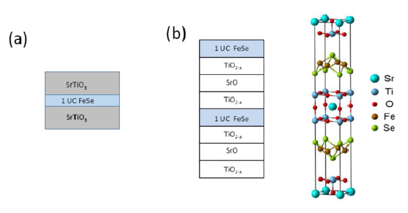
Figure 23: Possible FeSe/STO based superstructures, where the enhancement of $T_{c}$ can be expected DHL : (a) – Ginzburg’s “sandwich” with two STO layers, (b) – multiple layers superstructure.

Finally, let us discuss several proposals for possible ways of further increase of $T_{c}$ in FeSe monolayers on STO (or BTO) . If we accept the picture of decisive role of interactions with elementary excitations in the substrate (most probably with optical phonons), the natural idea appears of creation of multiple layer films and superstructures, like those shown in Fig. 23 DHL . In particular, the structure shown in Fig. 23 (a), is the direct realization of Ginzburg “sandwich”, precisely as was proposed in his original works VLG . It seems obvious, that the presence of the second SrTiO₃ layer (or the similar BaTiO₃ layer) will lead to the effective enhancement of the pairing constant due to interaction with optical phonons in the second STO layer. Obviously, the presence of the second STO layer will also serve as a good protection of FeSe layer from external environment. Similarly, very promising seems to be the attempts to create the bulk superstructures (compounds), like that shown in Fig. 23 (b). Despite all technical problems appearing on the way to create such structures (or their analogues), this way seems to be very perspective. There is no doubt that the last word in the studies of high – temperature superconductivity in FeSe monolayers and other similar systems is yet to be heard.

The author is grateful to E.Z. Kuchinskii and I.A. Nekrasov for discussions of the number of problems dealed with in this review, as well as for their help in some of numerical calculations.

This review was supported by RSF grant 14-12-00502. Calculations of electronic spectra of FeSe systems and comparative analysys of mechanisms of Cooper pairing were performed under FASO State contract No. 0389-2014-0001 with partial support by RFBR grant 14-02-00065.

Notes added in proof:

During the time after the submission of this review, a number of new experimental and theoretical works dealing with systems under discussion have appeared in the literature. Below we quote some of these with brief comments.

In Ref. Shi single – layer films of FeSe on STO were studied for different doping levels, which were achieved by surface deposition of potassium in situ. The sharp growth of $T_{c}$ from 60K to 75K was observed accompanied by Lifshits transition with formation of a small electron – like pocket of the Fermi surface around $\Gamma$ – point, which was confirmed by ARPES measurements. Note that such $T_{c}$ behavior is in complete accordance with qualitative conclusions of multiple – bands superconductivity theory, discussed in our review.

Important results were obtained in Ref. Shen , where the high values of $T_{c}\sim$65K were obtained for monolayers of FeSe on 100 plane of rutile TiO₂. These results show that ferroelectric properties of SrTiO₃ (absent for TiO₂) are irrelevant for $T_{c}$ growth in systems under disussion and almost unambiguously confirm the important role of interactions with longitudinal optical phonons in the substrate, which in TiO₂ are practically the same as in STO. Electronic spectrum of FeSe films on TiO₂ measured by ARPES was observed to be practically the same as in FeSe/STO, with “replica” band well observed approximately 100 meV below electronic band at $M$ – point, similar to that observed in Ref. [47] in FeSe/STO.

Experiments on high resolution electron energy loss spectroscopy (HREELS) performed in Ref. Zh confirmed the presence of strong electron – phonon interaction at FeSe/STO interface, giving the experimental estimate of coupling constant with 92 meV optical phonon in STO $\sim$ 1.0.

Theoretical results of Refs. [47,79] and [82,83] were critically reconsidered in Ref. Dolg . However, the qualitative conclusion on important role of dominating forward scattering of electron in FeSe monolayer by the optical phonons of SrTiO₃ for the increase of $T_{c}$ in FeSe/STO was essentially confirmed.

In Ref. John the “first principles” calculations of electron – phonon coupling if FeSe/STO system were performed, confirming the significant enhancement of this interaction in the region of small transferred momenta. However, the numerical values of corresponding coupling constant were too low to explain the experimentally observed high values of $T_{c}$. At the same time, it should be noted, that calculations of electronic spectrum for FeSe/STO sytem, performed in this work, were made neglecting the possible role of electron correlations, and spectra obtained were quite different from those observed in ARPES experiments (absence of the ”shallow“ band). Thus, the conclusions on the value of the coupling constant made in this work, may be rather approximate.

Gor’kov’s approach to explanation of superconductivity in SrTiO₃ [86] was criticized in Refs. Lee ; vdM . In principle, this criticism can can be extended to Refs. [84,85] dealing with superconductivity in FeSe/STO. At the same time, the use of phenomenological values of dielectric permeabilities at FeSe/STO interface in [84,85] makes the arguments of Refs. Lee ; vdM only partly relevant for this case.

Finally, we can mention the recent rather detailed review of experiments on intercalated A_xFe₂Se₂ systems Maziopa .

References

- (1) Ginzburg V L. Usp. Fiz. Nauk 95 91 (1968); 101 185 (1970); 118 316 (1976) [Contemporary Physics 9 355 (1968); Physics Uspekhi 13 535 (1970); 19 174 (1976)]
- (2) Problema visokotemperaturnoi sverkhprovodimosti. Ed. by V.L. Ginzburg and D.A. Kirzhits. GRFML “Nauka”, Moscow, 1977 [High – Temperature Superconductivity. Ed. by V.L. Ginzburg and D.A. Kirzhnits, Consultants Bureau, NY, 1982]
- (3) Sadovskii M V. Usp. Fiz. Nauk 178 1243 (2008) [Physics Uspekhi 51 1201 (2008)]
- (4) Ishida K, Nakai Y, Hosono H. J. Phys. Soc. Jpn. 78 062001 (2009)
- (5) Johnson D C, Adv. Phys. 59, 83 (2010)
- (6) Hirshfeld P J, Korshunov M M, Mazin I I. Rep. Prog. Phys. 74, 124508 (2011)
- (7) Stewart G R, Rev. Mod. Phys. 83, 1589 (2011)
- (8) Kordyuk A A, Fizika Nizkikh Temperatur 38 1119 (2012) [Low Temperature Physics 38 888 (2012)]
- (9) Mizugushi Y, Takano Y. J. Phys. Soc. Jpn. 79 102001 (2010)
- (10) Sadovskii M V, Kuchinskii E Z, Nekrasov N A. JMMM 324 3481 (2012)
- (11) Nekrasov I A, Sadovskii M V. Pis’ma Zh. Eksp. Teor. Fiz. 99 687 (2014) [JETP Letters99 598 (2014)]
- (12) Bozovic I, Ahn C. Nature Physics 10 892 (2014)
- (13) Vivanco H K, Rodriguez E E, ArXiv:1603.02334
- (14) Jiangang Guo, Shifeng Jin, Shunchong Wang, Kaixing Zhu, Tingting Zhou, Meng He, Xialong Chen. Phys. Rev. B 82 180520 (2010)
- (15) Yan Y J, Wang A F, Ying J J, Li Z Y, Qin W, Luo J Q, Hu J, Chen X H. Chin. Sci. Rep. 2 212 (2012)
- (16) Hatakeda T, Noji T, Kawamata T, Kato M, Koike Y. J. Phys. Soc. Jpn. 82 123705 (2013)
- (17) Burrad-Lucas M, Free D G, Sedlmaier S J, Wright J D, Cassidy S J, Hara Y, Corkett A J, Lancaster T, Baker P J, Blundell S J, Clarke S J. Nature Materials 12 15 (2013)
- (18) Lu X F, Wang N Z, Wu H, Wu Y P, Zhao D, Zeng X Z, Luo X G, Wu T, Bao W, Zhang G H, Huang F Q, Huang Q Z, Chen X H. Nature Materials 14 325 (2015)
- (19) Pachmayr U, Nitsche F, Luetkens H, Kamusella S, Brückner F, Sarkar R, Klauss H.-H, Johrendt D. Angew. Chem. Int. Ed. 54 293 (2015)
- (20) Lynn J W, Zhou X, Borg C K H, Saha S R, Paglione J, Rodriguez E E. Phys. Rev. B 92, 0605510(R) (2015)
- (21) Nejasattari F, Stadnik Z M. J. Alloys Compounds 652, 470 (2015)
- (22) Wang Qing-Yan, Li Zhi, Zhang Wen-Hao, Zhang Zuo-Cheng, Zhang Jin-Song, Li Wei, Ding Hao, Ou Yun-Bo, Deng Peng, Ghang Kai, Wen Jing, Song Can-Li, He Ke, Jia Jin-Feng, Ji Shuai-Hua, Wang Ya-Yu, Wang Li-Li, Chan Xi, Ma Xu-Cun, Xue Qi-Kun. Chin. Phys. Lett. 29 037402 (2012)
- (23) Jian-Feng Ge, Zhi-Long Liu, Chun-Lei Gao, Dong Qian, Qi-Kun Xue, Ying Liu, Jin-Feng Jia. Nature Materials 14 285 (2015)
- (24) Miyata Y, Nakayama K, Sugawara K, Sato T, Takahashi T. Nature Materials 14 775 (2015)
- (25) Guanyu Zhou, Ding Zhang, Chong Liu, Chenjia Tang, Xiaoxiao Wang, Zheng Li, Canli Song, Shuaihua Ji, Ke He, Lili Wang, Xucun Ma, Qi-Kun Xue. ArXiv:1512.01948
- (26) Peng R, Xu H C, Tan S Y, Xia M, Shan X P, Huang Z C, Wen C H P, Song Q, Zhang T, Xie B P, Feng D L. Nature Communications 5 5044 (2014)
- (27) Hao Ding, Yan-Feng Lv, Kun Zhao, Wen-Lin Wang, Lili Wang, Can-Li Song, Xi Chen, Xu-Cun Ma, Qi-Kun Xue. ArXiv:1603.00999
- (28) Can-Li Song, Yi-Lin Wang, Ye-Ping Jiang, Zhi Li, Lili Wang, Ke He, Xi Chen, Xu-Cun Ma, Qi-Kun Xue. Phys. Rev. B 84 020503(R) (2011)
- (29) Xu Liu, Lin Zhao, Shaolong He, Junfeng He, Defa Liu, Daixiang Mou, Bing Shen, Yong Hu, Jianwei Huang, Zhou X J. J. Phys. Cond. Mat. 27 183201 (2015)
- (30) Kuchinskii E Z, Sadovskii M V. Pis’ma Zh. Eksp. Teor. Fiz. 91 729 (2010) [JETP Letters 91 660 (2010)]
- (31) Skornyakov S L, Efremov A V, Skorikov N A, Korotin M A, Izyumov Yu A, Anisimov V I, Kozhevnikov A V, Vollhardt D. Phys. Rev. B 80 092501 (2009)
- (32) Nekrasov I A, Pavlov N S, Sadovskii M V. Pis’ma Zh. Eksp. Teor. Fiz. 102 30 (2015) [JETP Letters 102 26 (2015)]
- (33) Nekrasov I A, Sadovskii M V. Pis’ma Zh. Eksp. Teor. Fiz. 93 182 (2011) [JETP Letters 93 166 (2011)]
- (34) Shein I R, Ivanovskii A L. Phys. Lett. A 375 1028 (2011)
- (35) Nekrasov I A, Pchelkina Z V, Sadovskii M V. Pis’ma Zh. Eksp. Teor. Fiz. 88 155 (2008) [JETP Letters 88 144 (2008)]
- (36) Zhao L, Mou D, Liu S, He J, Peng Y, Yu L, Liu X, Liu G, He S, Dong X, Zhang J, He J B, Wang D M, Chen G F, Guo J G, Chen X L, Wang X, Peng Q, Wang Z, Zhang S, Yang F, Xu Z, Chen C, Zhou X J. Phys. Rev. B 83, 140508(R) (2011)
- (37) Nekrasov I A, Pavlov N S, Sadovskii M V. Pis’ma Zh. Eksp. Teor. Fiz. 97 18 (2013) [JETP Letters 97 15 (2013)]
- (38) Nekrasov I A, Pavlov N S, Sadovskii M V. Zh. Eksp. Teor. Fiz. 144 1061 (2013) [JETP 117 926 (2013)]
- (39) Nekrasov I A, Pavlov N S, Sadovskii M V, Pis’ma Zh. Eksp. Teor. Fiz. 95 659 (2012) [JETP Letters 95 581 (2012)]
- (40) Nekrasov I A, Pavlov N S, Sadovskii M V, Zh. Eksp. Teor. Fiz. 143 713 (2013) [JETP 116 620 (2013)]
- (41) Yi M, Lu D H, Yu R, Riggs S C, Chu J H, Lv B, Liu Z K, Lu M, Cui Y T, Hashimoto M, Mo S K, Hussain Z, Chu C W, Fisher I R, Si Q, Shen Z X, Phys. Rev. Lett. 110 067003 (2013)
- (42) Niu X H, Chen S D, Jiang J, Ye Z R, Yu T L, Xu D F, Xu M, Feng Y, Yan Y J, Xie B P, Zhao J, Gu D C, Sun L L, Mao Q, Wang H, Fang M, Zhang C J, Hu J P, Sun Z, Feng D L. Phys. Rev. B 93 054516 (2016)
- (43) Nekrasov I A, Sadovskii M V. Pis’ma Zh. Eksp. Teor. Fiz. 101 50 (2015)
- (44) Niu X H, Peng R, Xu H C, Yan Y J, Jiang J, Xu D F, Yu T L, Song Q, Huang Z C, Wang Y X, Xie B P, Lu X F, Wang N Z, Chen X H, Sun Z, Feng D L. Phys. Rev. B 92 060504(R) (2015)
- (45) Nekrasov I A, Pavlov N S, Sadovskii M V, Slobodchikov A.A. ArXiv:1605.02404
- (46) Defa Liu, Wenhao Zhang, Daixiang Mou, Junfeng He, Yun-Bo Ou, Qing-Yan Wang, Zhi Li, Lili Wang, Lin Zhao, Shaolong He, Yingying Peng, Xu Liu, Chaoyu Chen, Li Yu, Guodong Liu, Xiaoli Dong, Jun Zhang, Chuangtian Chen, Zuyan Xu, Jiangping Hu, Xi Chen, Xucun Ma, Qikun Xue, X. J. Zhou. Nature Communications 3, 931 (2012)
- (47) Lee J J, Schmitt F T, Moore R G, Johnston S, Cui Y T, Li W, Liu Z K, Hashimoto M, Zhang Y, Lu D H, Devereaux T P, Lee D H, Shen Z X. Nature 515, 245 (2014)
- (48) Lin Zhao, Aiji Liang, Dongna Yuan, Yong Hu, Defa Liu, Jianwei Huang, Shaolong He, Bing Shen, Yu Xu, Xu Liu, Li Yu, Guodong Liu, Huaxue Zhou, Yulong Huang, Xiaoli Dong, Fang Zhou, Zhongxian Zhao, Chuangtian Chen, Zuyan Xu, Zhou X J. Nature Communications 7, 10608 (2016)
- (49) Han Fu, Reich K V, Shklovskii B I. Zh. Eksp. Teor. Fiz. 130 530 (2016) [JETP 122 No.3 (2016)]
- (50) Yuanjun Zhou, Mills A J. ArXiv:1603.02728
- (51) Chen M X, Agterberg D F, Weinert M. ArXiv:1603.03841
- (52) Shaolong He, Junfeng He, Wenhao Zhang, Lin Zhao, Defa Liu, Xu Liu, Daixiang Mou, Yun-Bo Ou, Qing-Yan Wang, Zhi Li, Lili Wang, Yingying Peng, Yan Liu, Chaoyu Chen, Li Yu, Guodong Liu, Xiaoli Dong, Jun Zhang, Chuangtian Chen, Zuyan Xu, Xi Chen, Xucun Ma, Qikun Xue, Zhou X J. Nature Materials 12 605 (2013)
- (53) Junfeng He, Xu Liu, Wenhao Zhang, Lin Zhao, Defa Liu, Shaolong He, Daixiang Mou, Fansen Li, Chenjia Tang, Zhi Li, Lili Wang, Yingying Peng, Yan Liu, Chaoyu Chen, Li Yu, Guodong Liu, Xiaoli Dong, Jun Zhang, Chuangtian Chen, Zuyan Xu, Xi Chen, Xucun Ma, Qikun Xue, Zhou X J, PNAS 111 18501 (2014)
- (54) Mizuguhci Y, Hara Y, Deguchi K, Tsuda S, Yamaguchi T, Takeda K, Kotegawa H, Tou H, Takano Y, Supercond. Sci. Technol. 23 054013 (2010)
- (55) Kuchinskii E Z, Nekrasov I A, Sadovskii M V, Pis’ma Zh. Eksp. Teor. Fiz. 91 567 (2010) [JETP Letters 91 518 (2010)]
- (56) Miyata Y, Nakayama K, Sugawara K, Sato T, Takahashi T. Nature Materials 14 775 (2015)
- (57) Wen C H P, Xu H C, Chen C, Huang Z C, Pu Y J, Song Q, Xie B P, Abdel-Hafez M, Chareev D A, Vasiliev A N, Peng R, Feng D L. Nature Communications 7 10840 (2016)
- (58) Ye Z R, Zhang C F, Ning H L, Li W, Chen L, Jia T, Hashimoto M, Lu D H, Shen Z X, Zhang Y. ArXiv:1512.02526
- (59) Fawei Zheng, Li-Li Wang, Qi-Kun Xue, Ping Zhang. Phys. Rev. B 93 075428
- (60) Shiogai J, Ito Y, Mitsuhashi T, Nojima T, Tsukazaki A. Nature Physics 12 42 (2016)
- (61) Hanzawa K, Sato H, Hiramatsu T, Hosono H. ArXiv:1508.07689; PNAS (2016); DOI:10.1073/pnas.1520810113
- (62) Lei B, Chui J H, Xiang Z J, Shang C, Wang N Z, Ye G J, Luo X G, Wu T, Sun Z, Chen X H. Phys. Rev. Lett. 116 077002 (2016)
- (63) Barzykin V, Gor’kov L P. 88 142 (2008) [JETP Letters 88 131 (2008)]
- (64) Kuchinskii E Z, Sadovskii M V. 89 176 (2009) [JETP Letters 89 156 (2009)]
- (65) Xiao Chen, Maiti S, Linschfeld A, Hirschfeld P J. Phys. Rev. B 92 224514 (2015)
- (66) Kuchinskii E Z, Sadovskii M V. Physica C 470 S418 (2010)
- (67) Sat T, Nakayama K, Sekiba Y, Richard P, Xu Y M, Souma S, Takahashi T, Chen G F, Luo J L, Wang N L, Ding H. Phys. Rev. Lett. 103 047002 (2009)
- (68) Sekiba Y, Sato T, Nakayama K, Terashima K, Richard P, Bowen J H, Ding H, Xu Y M, Li L J, Gao G H, Xu Z A, Takahashu T. New J. Phys. 11 025020 (2009)
- (69) Fan Q, Zhang W H, Liu X, Yan Y J, Ren M Q, Peng R, Xu H C, Xie B P, Hu J P, Zhang T, Feng D L. Nature Physics 11 946 (2015)
- (70) van Benthem K, Elsässer C, French R H. J. Appl. Phys. 90 6156 (2001)
- (71) Müller K A, Burkard H. Phys. Rev. B 19 3593 (1979)
- (72) Koonce C S, Cohen M L, Schooley J F, Hosler W R, Pfeiffer E R. Phys. Rev 163 380 (1967)
- (73) Lin X, Zhu Z, Fauqué, Behnia K. Phys. Rev. X 021002 (2013)
- (74) Allender D, Bray J, Bardeen J. Phys. Rev. B 7 1020 (1973)
- (75) Inkson J C, Anderson P W. Phys. Rev. B 8 4429 (1973)
- (76) Uspenskii Y A, Zharkov G F. Zh. Eksp. Teor. Fiz 65 2511 (1974) [JETP 38 1254 (1974)]
- (77) Allender D, Bray J, Bardeen J. Phys. Rev. B 8 4433 (1973)
- (78) Choudhury N, Walter E J, Kolesnikov A I, Chun-Keung Loong. Phys. Rev. B 77 134111 (2008)
- (79) Dung-Hai Lee. ArXiv:1508.02461
- (80) Danylenko O V, Dolgov O V, Kulić M L, Oudovenko V. Eur. J. Phys. B 9 201 (1999)
- (81) Kulić M L, AIP Conference Proceedings 715 75 (2004)
- (82) Rademaker L, Wang Y, Berlijn T, Johnston S. New J. Phys. 18 022001 (2016)
- (83) Wang Y, Nakatsukasa K, Rademaker L, Berlijn T, Johnston S. ArXiv:1602.00656
- (84) Gor’kov L P. Phys. Rev. B 93 060507 (2016)
- (85) Gor’kov L P. Phys. Rev. B 93 054517 (2016)
- (86) Gor’kov L P. PNAS 113 4646 (2016); ArXiv:1508.00529
- (87) Wang S Q, Mahan G D. Phys. Rev. B 6 4517 (1972)
- (88) Nozieres P, Schmitt-Rink S. J. Low. Temp. Phys. 59 195 (1985)
- (89) Randeria M. In “Bose-Einstein Condensation”, Eds. A. Griffin, D. W. Snoke, S. Stringari. Cambridge University Press, 1995, p. 355
- (90) Lubashevsky Y, Lahoud E, Chashka K, Podolsky D, Kanigel A. Nature Physics 8 309 (2012)
- (91) Kasahara S, Watashige T, Hanaguri T, Kohsaka Y, Yamashita T, Shimoyama Y, Mizukami Y, Endo R, Ikeda H, Aoyama K, Terashima T, Uji S, Wolf T, Löhneysen H v, Shibauchi T, Matsuda Y. PNAS 111 16309 (2014)
- (92) Chubukov A V, Eremin I, Efremov D V. ArXiv:1601.01678

References

- (1) Shi X, Han Z.-Q, Peng X.-L, Richard P, Qian T, Wu X.-X, Qiu M.-W, Wang S C, Hu J P, Sun Y,-J, Ding H. ArXiv:1606.01470
- (2) Rebec S N, Jia T, Zhang C, Hashimoto M, Lu D.-H, Moore R G, Shen Z.-X. ArXiv:1606.09358
- (3) Zhang S, Guan J, Jia X, Liu B, Wang W, Li F, Wang L, Ma X, Xue Q, Zhang J, Plummer E W, Zhu X, Guo J. ArXiv:1605.06941
- (4) Kulic M L, Dolgov O V. ArXiv:1607.00843
- (5) Wang Y, Linscheld A, Berlijn T, Johnson S. ArXiv:1602.03288
- (6) Ruhman J, Lee P A. ArXiv:1605.01737
- (7) Klimin S N, Tempere J, Devreese J T, van der Marel D. ArXiv:1606.00644
- (8) Krzton-Maziopa A, Svitlyk V, Pomjakushina E, Puzniak R. J. Phys. Condens. Matter 28 293002 (2016)