An introduction to Multitrace Formulations and Associated Domain Decomposition Solvers

Abstract

Multitrace formulations (MTFs) are based on a decomposition of the problem domain into subdomains, and thus domain decomposition solvers are of interest. The fully rigorous mathematical MTF can however be daunting for the non-specialist. We introduce in this paper MTFs on a simple model problem using concepts familiar to researchers in domain decomposition. This allows us to get a new understanding of MTFs and a natural block Jacobi iteration, for which we determine optimal relaxation parameters. We then show how iterative multitrace formulation solvers are related to a well known domain decomposition method called optimal Schwarz method: a method which used Dirichlet to Neumann maps in the transmission condition. We finally show that the insight gained from the simple model problem leads to remarkable identities for Calderón projectors and related operators, and the convergence results and optimal choice of the relaxation parameter we obtained is independent of the geometry, the space dimension of the problem, and the precise form of the spatial elliptic operator, like for optimal Schwarz methods. We illustrate our analysis with numerical experiments.

1 Introduction

Multitrace formulations (MTF) for boundary integral equations (BIE) were developed over the last few years, see [15, 2, 3], for the simulation of electromagnetic transmission problems in piecewise constant media, and also [4] for associated boundary integral methods. MTFs are naturally adapted to the development of new block preconditioners, as indicated in [16], but very little is known so far about such associated iterative domain decomposition solvers. The first goal of our presentation (see Section 2) is to give an elementary introduction to MTFs, and the associated concepts of representation formulas and Calderón projectors for a simple model problem in one spatial dimension, in order to make these concepts accessible for people working in domain decomposition. This approach allows us to get a complete understanding of the performance of a block Jacobi iteration for the MTF applied to our model problem, and to determine the influence of the relaxation parameter on the convergence of the block Jacobi method. Based on these results, we establish in Section 3 an interesting connection between MTFs with a well studied class of domain decomposition methods called optimal Schwarz methods, see [18, 10, 11, 12, 13], and [9] for an overview with further references. Optimal Schwarz methods use Dirichlet to Neumann operators in their transmission conditions, and are very much related to the very recent class of sweeping preconditioners, [7, 6], see also the earlier work on the same method known under the name AILU (Analytic Incomplete LU factorization) in [8, 14], or frequency filtering [20]. To find the connection with MTFs, we need to generalize first the MTF to the case of bounded domains and give a formulation of the Calderón projectors in terms of the Dirichlet to Neumann and Neumann to Dirichlet operators. We then show in Section 4 that the insight gained for the one dimensional problem holds in much more general situations. It allows us to discover remarkable properties of the Calderón projector and related operators in higher spatial dimensions and on various geometries, and the performance of the block Jacobi iteration and the dependence on the relaxation parameter remain as we discovered for the one dimensional model problem. We illustrate our results with numerical experiments that confirm our analysis.

2 Multitrace Formulations for a Simple 1D Model Problem

Because multitrace formulations need substantial knowledge in functional analysis, representation formulas and Calderón projectors, we start in this section by explaining these concepts for a simple model problem in one spatial dimension, without dwelling on functional analysis issues. The more general formulation and associated functional analysis framework will be introduced in Section 4.

2.1 Representation Formulas in 1D

We start by examining for some given constant $a>0$ solutions of the differential equation

$$\left\{\begin{array}[]{rcl}\displaystyle-\frac{d^{2}u}{dx^{2}}+a^{2}u&=&0,\quad\textrm{in}\;\mathbb{R}\setminus\{0\},\\ \displaystyle\lim_{|x|\rightarrow\infty}|u(x)|&=&0.\end{array}\right.$$ (1)

Since the domain on which the equation holds excludes the point $x=0$, there are non-zero solutions, and to select a particular one, two more conditions must be imposed on the solution at $x=0$. In transmission problems and multitrace formulations, one works with solutions that can be discontinuous, and we thus introduce the notation of jumps (with convention that the orientation is from $\mathbb{R}_{+}$ to $\mathbb{R}_{-}$),

$$\begin{array}[]{rcl}\displaystyle[u]&:=&u(0_{+})-u(0_{-}),\\ \displaystyle\left[\frac{du}{dx}\right]&:=&\displaystyle-\frac{du}{dx}(0_{+})+\frac{du}{dx}(0_{-}).\end{array}$$ (2)

Imposing both jumps at $x=0$ selects a unique solution of (1); solving for example the case where the solution is continuous, but has a jump of size $\beta$ in the derivative,

$$\left\{\begin{array}[]{rcl}\displaystyle-\frac{d^{2}u}{dx^{2}}+a^{2}u&=&0,\quad\textrm{in}\;\mathbb{R}\setminus\{0\},\\ \displaystyle[u]&=&0,\\ \displaystyle\left[\frac{du}{dx}\right]&=&\beta,\\ \displaystyle\lim_{x\rightarrow\infty}|u(x)|&=&0,\end{array}\right.$$ (3)

we obtain as solution decaying exponentials in each part of the domain and conditions determining the constants,

$$\begin{array}[]{rcl}u(x)&=&c_{+}e^{-ax}\mathbf{1}_{\mathbb{R}_{+}}+c_{-}e^{ax}\mathbf{1}_{\mathbb{R}_{-}},\\ c_{+}-c_{-}&=&0,\\ a(c_{+}+c_{-})&=&\beta.\end{array}$$

Solving the linear system for the constants, we find $c_{\pm}=\beta/(2a)$ and hence our solution can be written in compact form with the so called Green’s function $\mathcal{G}$ as

$$u(x)=\beta\,\mathcal{G}(x),\quad\quad\mathcal{G}(x):=\frac{e^{-a|x|}}{2a}.$$ (4)

If we impose instead a jump $\alpha$ in the solution, but continuous derivatives,

$$\left\{\begin{array}[]{rcl}\displaystyle-\frac{d^{2}u}{dx^{2}}+a^{2}u&=&0,\,\mathbb{R}\setminus\{0\},\\ \displaystyle[u]&=&\alpha,\\ \displaystyle\left[\frac{du}{dx}\right]&=&0,\\ \displaystyle\lim_{x\rightarrow\infty}|u(x)|&=&0.\end{array}\right.$$ (5)

we find by similar calculations

$$u(x)=\frac{\alpha}{2}\text{sign}(x)e^{-a|x|}=-\alpha\frac{d\mathcal{G}}{dx}(x),$$ (6)

where $\mathcal{G}$ is again the Green’s function from (4). By linearity, any function $u(x)$ solution to (1) with Dirichlet jump $[u]=\alpha$ and Neumann jump $[du/dx]=\beta$ is thus given by the formula

$$\boxed{u(x)=\left[\frac{du}{dx}\right]{\cal G}(x)-[u]\frac{d{\cal G}(x)}{dx},\quad\quad\forall x\in\mathbb{R}\setminus\{0\}.}$$ (7)

This formula is called representation formula for the solution.

2.2 Calderón Projectors in 1D

If $u$ is any function satisfying $-d^{2}u/dx^{2}+a^{2}u=0$ on $\mathbb{R}_{+}$ and $u(x)\to 0$ for $x\to\infty$, then we can extend the function by zero on the negative real axis, $u(x)=0$ for $x<0$, and it then satisfies (1). Hence the representation formula (7) yields $u(x)=(G_{+}\circ T_{+}(u))(x)$ for $x\in\mathbb{R}_{+}$, where

$$G_{+}\left(\begin{array}[]{c}\alpha\\ \beta\end{array}\right):=-\alpha\frac{d{\cal G}(x)}{dx}+\beta\,{\cal G}(x)\;,\quad\quad T_{+}(u):=\left(\begin{array}[]{c}u(0_{+})\\ -\frac{du}{dx}(0_{+})\end{array}\right).$$ (8)

Observe that the composition in the reverse order, $T_{+}\circ G_{+}$, is here a simple $2\times 2$ matrix whose coefficients can be explicitly computed from the expression of the Green’s function $\mathcal{G}$ given in (4). This yields

$$\mathbb{P}_{+}:=T_{+}\circ G_{+}=\frac{1}{2}\Big{(}\operatorname{I}+\underbrace{\left[\begin{array}[]{cc}0&1/a\\ a&0\end{array}\right]}_{A}\Big{)},\quad\quad A^{2}=\operatorname{I}\quad\Longrightarrow\quad\mathbb{P}_{+}^{2}=\mathbb{P}_{+}.$$ (9)

We therefore see that $\mathbb{P}_{+}$ is a projector, which is called Calderón projector associated with $\mathbb{R}_{+}$.

Similarly, if $u$ is any function satisfying $-d^{2}u/dx^{2}+a^{2}u=0$ on $\mathbb{R}_{-}$ and $u(x)\to 0$ for $x\to-\infty$ then, setting $u(x)=0$ for $x>0$, the representation formula (7) can be applied which yields $u(\boldsymbol{x})=(G_{-}\circ T_{-}(u))(\boldsymbol{x})$ for $\boldsymbol{x}\in\mathbb{R}_{-}$ with

$$G_{-}\left(\begin{array}[]{c}\alpha\\ \beta\end{array}\right):=\alpha\frac{d{\cal G}(x)}{dx}+\beta\,{\cal G}(x)\;,\quad\quad T_{-}(u):=\left(\begin{array}[]{c}u(0_{-})\\ \frac{du}{dx}(0_{-})\end{array}\right).$$ (10)

Computing $\mathbb{P}_{-}:=T_{-}\circ G_{-}$ in the same manner as above, we find that $\mathbb{P}_{-}=(\operatorname{I}+A)/2$ with the same matrix $A$ as in (9), and $\mathbb{P}_{-}^{2}=\mathbb{P}_{-}$ is the Calderón projector associated with $\mathbb{R}_{-}$.

Remark 1.

We see that the Calderón projector performs a very simple operation: it takes two arbitrary jumps along the interface, solves the coupled transmission problem with these jumps, and then returns the Dirichlet and Neumann trace of the domain the Calderón projector is associated with.

2.3 Multitrace Formulation with 2 Subdomains in 1D

Suppose now we have a decomposition of $\mathbb{R}$ into two subdomains $\Omega_{1}=\mathbb{R}_{-}$ and $\Omega_{2}=\mathbb{R}_{+}$. Let $T_{1,2}$ be the trace operators as defined in (8) and (10) ($T_{1}=T_{-}$ and $T_{2}=T_{+}$) for the subdomains $\Omega_{1,2}$, and let $\mathbb{P}_{1,2}$ be the corresponding Calderón projectors as defined in (9) ($\mathbb{P}_{1}=\mathbb{P}_{-}=:\mathbb{P}$ and $\mathbb{P}_{2}=\mathbb{P}_{+}=\mathbb{P}$). Suppose we want to solve the transmission problem

$$\left\{\begin{array}[]{l}\displaystyle-\frac{d^{2}u}{dx^{2}}+a^{2}u=0,\quad\textrm{in}\;\mathbb{R}\setminus\{0\},\\ \displaystyle[u]=\alpha,\quad\left[\frac{du}{dx}\right]=\beta,\\ \displaystyle\lim_{|x|\rightarrow-\infty}u(x)=0.\end{array}\right.$$ (11)

The multitrace formulation introduced in [15], which we present in the form with relaxation parameters from [16] states that $u$ is solution to (11) if its traces $U_{1,2}:=(T_{i}u)_{i=1,2}$ verify the relations

$$\left\{\begin{array}[]{l}(\operatorname{I}-\mathbb{P}_{1})U_{1}+\sigma_{1}\left(U_{1}-XU_{2}\right)=F_{1},\\[5.0pt] (\operatorname{I}-\mathbb{P}_{2})U_{2}+\sigma_{2}\left(U_{2}-XU_{1}\right)=F_{2},\end{array}\right.$$ (12)

where $F_{1}=\sigma_{1}\cdot(-\alpha,\beta)^{T}$, $F_{2}=\sigma_{2}\cdot(\alpha,\beta)^{T}$, $\sigma_{1},\sigma_{2}\in\mathbb{C}$ are some relaxation parameters, and

$$X:=\left(\begin{array}[]{cc}1&0\\ 0&-1\end{array}\right).$$ (13)

We see that (12) clearly holds for the solution $u$: first $(\operatorname{I}-\mathbb{P}_{j})U_{j}=0$ by Remark 1, since applying the Calderón projector to a solution just gives the solution itself. Second, the relaxation term on the left gives precisely the jumps weighted by the relaxation, which we also find in the right hand side functions $F_{j}$ which contain as data the jumps $\alpha$, $\beta$ of the transmission problem. Note also that this formulation would not make sense for vanishing relaxation parameters, $\sigma_{j}=0$, $j=1,2$, since then the jump data $\alpha$, $\beta$ disappear from the problem formulation.

Collecting the operators that act on the same trace variables $U_{j}$, we can rewrite (12) in matrix form as a $4\times 4$ linear system of equations, namely

$$\left[\begin{array}[]{cc}(1+\sigma_{1})\operatorname{I}-\mathbb{P}_{1}&-\sigma_{1}X\\ -\sigma_{2}X&(1+\sigma_{2})\operatorname{I}-\mathbb{P}_{2}\end{array}\right]\left[\begin{array}[]{c}U_{1}\\ U_{2}\end{array}\right]=\left[\begin{array}[]{c}F_{1}\\ F_{2}\end{array}\right].$$ (14)

A very natural iterative method to solve this linear system would be a block-Jacobi iteration,

$$\left[\begin{array}[]{c}U_{1}\\ U_{2}\end{array}\right]^{n+1}=J_{2}\left[\begin{array}[]{c}U_{1}\\ U_{2}\end{array}\right]^{n}+\tilde{F},$$ (15)

where the associated iteration matrix is

$$J_{2}=\left[\begin{array}[]{cc}(1+\sigma_{1})\operatorname{I}-\mathbb{P}_{1}&0\\ 0&(1+\sigma_{2})\operatorname{I}-\mathbb{P}_{2}\end{array}\right]^{-1}\left[\begin{array}[]{cc}0&\sigma_{1}X\\ \sigma_{2}X&0\end{array}\right].$$ (16)

Using the explicit formulas (9) for the Calderón projectors, we can compute explicitly

$$J_{2}=\displaystyle\left[\begin{array}[]{cccc}0&0&\frac{2\sigma_{1}+1}{2(\sigma_{1}+1)}&-\frac{1}{2a(\sigma_{1}+1)}\\ 0&0&\frac{a}{2(\sigma_{1}+1)}&-\frac{2\sigma_{1}+1}{2(\sigma_{1}+1)}\\ \frac{2\sigma_{2}+1}{2(\sigma_{2}+1)}&-\frac{1}{2a(\sigma_{2}+1)}&0&0\\ \frac{a}{2(\sigma_{2}+1)}&-\frac{2\sigma_{2}+1}{2(\sigma_{2}+1)}&0&0\end{array}\right],$$ (17)

and the right hand side function is

$$\tilde{F}=\left[\begin{array}[]{c}-\frac{a\alpha(2\sigma_{1}+1)-\beta}{2a(1+\sigma_{1})}\\ -\frac{a\alpha-\beta(2\sigma_{1}+1)}{2(1+\sigma_{1})}\\ \frac{a\alpha(2\sigma_{2}+1)+\beta}{2a(1+\sigma_{2})}\\ \frac{a\alpha+\beta(2\sigma_{2}+1)}{2(1+\sigma_{2})}\end{array}\right].$$ (18)

The convergence factor of the block Jacobi iteration (15) is given by the spectral radius of the iteration matrix $J_{2}$, whose spectrum can be easily computed,

$$\sigma(J_{2})=\left\{-\sqrt{\frac{\sigma_{1}}{\sigma_{1}+1}},\sqrt{\frac{\sigma_{1}}{\sigma_{1}+1}},-\sqrt{\frac{\sigma_{2}}{\sigma_{2}+1}},\sqrt{\frac{\sigma_{2}}{\sigma_{2}+1}}\right\}.$$ (19)

We note that the eigenvalues are independent of the problem parameter $a$ and thus the convergence speed of the method only depends on the relaxation parameters $\sigma_{j}$. This implies that the convergence would be independent of the Fourier variable and thus robust when the mesh size is refined in a two dimensional setting, as it was pointed out in [5]. Plotting the modulus of the eigenvalues as function of $\sigma_{j}$, we obtain the result in Figure 1.

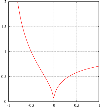
Fig. 1: Eigenvalues in modulus of the block Jacobi iteration matrix as a function of the relaxation parameter $\sigma_{j}$

We see that the algorithm diverges for $\sigma_{j}<-0.5$, stagnates for $\sigma_{j}=-0.5$ and converges for all others values of $\sigma_{j}$. For $\sigma_{j}$ close to zero, convergence is very rapid, and for $\sigma_{j}=0$, $j=1,2$, the spectral radius of the iteration matrix vanishes, which would make the method a direct solver, since the iteration matrix becomes nil-potent. We have seen however also that for vanishing relaxation parameters, the multitrace formulation (12) does not make sense any more, since the jump data is not contained any more in the formulation. Nevertheless, the associated block Jacobi iteration for the multitrace formulation (12) is well defined in the limit as $\sigma_{j}$ goes to zero for $j=1,2$, and we get from (17)

$$\lim_{\sigma_{j}=0}J_{2}=\displaystyle\left[\begin{array}[]{cccc}0&0&\frac{1}{2}&-\frac{1}{2a}\\ 0&0&\frac{a}{2}&-\frac{1}{2}\\ \frac{1}{2}&-\frac{1}{2a}&0&0\\ \frac{a}{2}&-\frac{1}{2}&0&0\end{array}\right]=\left[\begin{array}[]{cc}0&\mathbb{P}X\\ \mathbb{P}X&0\end{array}\right].$$ (20)

The limit of the right hand side (18) is also well defined, containing the data

$$\lim_{\sigma_{j}=0}\tilde{F}=\left[\begin{array}[]{c}-\frac{a\alpha-\beta}{2a}\\ -\frac{a\alpha-\beta}{2}\\ \frac{a\alpha+\beta}{2a}\\ \frac{a\alpha+\beta}{2}\end{array}\right]=\left[\begin{array}[]{c}-\mathbb{P}X\left[\begin{array}[]{c}\alpha\\ \beta\end{array}\right]\\ \mathbb{P}\left[\begin{array}[]{c}\alpha\\ \beta\end{array}\right]\end{array}\right].$$

Therefore the block Jacobi iteration is also well defined in the limit $\sigma_{j}=0$,

$$\left[\begin{array}[]{c}U_{1}\\ U_{2}\end{array}\right]^{n+1}=\left[\begin{array}[]{cc}0&\mathbb{P}X\\ \mathbb{P}X&0\end{array}\right]\left[\begin{array}[]{c}U_{1}\\ U_{2}\end{array}\right]^{n}+\left[\begin{array}[]{c}-\mathbb{P}X[\alpha,\beta]^{T}\\ \mathbb{P}[\alpha,\beta]^{T}\end{array}\right],$$ (21)

and this iteration defines us at convergence a new multitrace formulation

$$\begin{array}[]{rcl}U_{1}-\mathbb{P}XU_{2}&=&-\mathbb{P}X[\alpha,\beta]^{T},\\ U_{2}-\mathbb{P}XU_{1}&=&\mathbb{P}[\alpha,\beta]^{T}.\end{array}$$ (22)

The advantage of this multitrace formulation is that it is already preconditioned, block Jacobi applied to it is optimal in the sense that convergence is achieved in a finite number of steps. A direct calculation shows that $J_{2}^{2}$ equals zero, and thus convergence is achieved in at most 2 iterations. We will see in Section 3 that this iteration corresponds to a well-known algorithm in domain decomposition.

2.4 Multitrace Formulation for 3 Subdomains in 1D

We consider now a decomposition into three subdomains: $I_{1}=(-\infty,-1)$, $I_{0}=(-1,1)$ and $I_{2}=(1,\infty)$, and functions that satisfy

$$\left\{\begin{array}[]{rcl}\displaystyle-\frac{d^{2}u}{dx^{2}}+a^{2}u&=&0,\,\mathbb{R}\setminus\{\pm 1\},\\ \displaystyle\lim_{x\rightarrow\infty}|u(x)|&=&0.\end{array}\right.$$ (23)

If we denote the restriction of the solution onto the subdomains by $u_{j}=u|_{I_{j}}$, $j=0,1,2$, then by using a similar reasoning as in the two-subdomain case in Subsection 2.1, we obtain the representation formula

$$\begin{array}[]{rcl}u(x)&=&\displaystyle\left[-\frac{du_{0}}{dx}(-1)+\frac{du_{1}}{dx}(-1)\right]{\cal G}(x+1)+\left[\frac{du_{0}}{dx}(1)-\frac{du_{2}}{dx}(1)\right]{\cal G}(x-1)\\ &-&\displaystyle[u_{0}(-1)-u_{1}(-1)]\frac{d{\cal G}}{dx}(x+1)+[u_{0}(1)-u_{2}(1)]\frac{d{\cal G}}{dx}(x-1)\\ &=&\displaystyle\left[-\frac{du}{dx}\right]_{-1}\frac{e^{-a|x+1|}}{2a}+\left[\frac{du}{dx}\right]_{1}\frac{e^{-a|x-1|}}{2a}\\ &+&\displaystyle[u]_{-1}\text{sign}(x+1)\frac{e^{-a|x+1|}}{2}-[u]_{1}\text{sign}(x-1)\frac{e^{-a|x-1|}}{2},\end{array}$$ (24)

where we defined the jumps of the derivatives to be

$$\beta_{-1}:=\left[-\frac{du}{dx}\right]_{-1}:=-\frac{du_{0}}{dx}(-1)+\frac{du_{1}}{dx}(-1),\quad\beta_{1}:=\left[\frac{du}{dx}\right]_{1}:=\left[\frac{du_{0}}{dx}(1)-\frac{du_{2}}{dx}(1)\right],$$

and the jumps in the function values are

$$\alpha_{-1}:=[u]_{-1}:=u_{0}(-1)-u_{1}(-1),\quad\alpha_{1}:=[u]_{1}:=u_{0}(1)-u_{2}(1).$$

Suppose now that we want to compute the Calderón projector for the domain $I_{0}$. From (24) we see that for $x\in I_{0}$ we have

$$\begin{array}[]{rcl}u_{0}(x)&=&\displaystyle\alpha_{-1}\frac{e^{-a(x+1)}}{2}+\beta_{-1}\frac{e^{-a(x+1)}}{2a}+\alpha_{1}\frac{e^{a(x-1)}}{2}+\beta_{1}\frac{e^{a(x-1)}}{2a}\\ &=&\displaystyle\displaystyle a\alpha_{-1}{\cal G}(x+1)+\beta_{-1}{\cal G}(x+1)+a\alpha_{1}{\cal G}(x-1)+\beta_{1}{\cal G}(x-1),\\[8.61108pt] \displaystyle\frac{du_{0}}{dx}(x)&=&\displaystyle-a\alpha_{-1}\frac{e^{-a(x+1)}}{2}-\beta_{-1}\frac{e^{-a(x+1)}}{2}+a\alpha_{1}\frac{e^{a(x-1)}}{2}+\beta_{1}\frac{e^{a(x-1)}}{2}\displaystyle\\ &=&\displaystyle\displaystyle-a^{2}\alpha_{-1}{\cal G}(x+1)-a\beta_{-1}{\cal G}(x+1)+a^{2}\alpha_{1}{\cal G}(x-1)+a\beta_{1}{\cal G}(x-1).\end{array}$$ (25)

If we define the Cauchy trace by

$$T_{0}(u)=\left[u_{0}(-1),-\frac{du_{0}}{dx}(-1),u_{0}(1),\frac{du_{0}}{dx}(1)\right]^{T},$$

then from the formula (25) we obtain

$$\begin{array}[]{rcl}u_{0}(-1)&=&\displaystyle\alpha_{-1}\frac{1}{2}+\beta_{-1}\frac{1}{2a}+a\alpha_{1}{\cal G}(-2)+\beta_{1}{\cal G}(-2),\\ \displaystyle-\frac{du_{0}}{dx}(-1)&=&\displaystyle\alpha_{-1}\frac{a}{2}+\beta_{-1}\frac{1}{2}-a^{2}\alpha_{1}{\cal G}(-2)-a\beta_{1}{\cal G}(-2),\\ u_{0}(1)&=&\displaystyle a\alpha_{-1}{\cal G}(2)+\beta_{-1}{\cal G}(2)+\alpha_{1}\frac{1}{2}+\beta_{1}\frac{1}{2a},\\ \displaystyle\frac{du_{0}}{dx}(1)&=&\displaystyle-a^{2}\alpha_{-1}{\cal G}(2)-a\beta_{-1}{\cal G}(2)+\alpha_{1}\frac{a}{2}+\beta_{1}\frac{1}{2},\end{array}$$

and thus using the short hand notation $g_{\pm}:={\cal G}(\pm 2)$

$$T_{0}(u)=\left[\begin{array}[]{cccc}\frac{1}{2}&\frac{1}{2a}&ag_{-}&g_{-}\\ \frac{a}{2}&\frac{1}{2}&-a^{2}g_{-}&-ag_{-}\\ ag_{+}&g_{+}&\frac{1}{2}&\frac{1}{2a}\\ -a^{2}g_{+}&-ag_{+}&\frac{a}{2}&\frac{1}{2}\end{array}\right]\left(\begin{array}[]{c}\alpha_{-1}\\ \beta_{-1}\\ \alpha_{1}\\ \beta_{1}\end{array}\right)=:\mathbb{P}_{0}\left(\begin{array}[]{c}\alpha_{-1}\\ \beta_{-1}\\ \alpha_{1}\\ \beta_{1}\end{array}\right).$$ (26)

Here $\mathbb{P}_{0}$ is the Calderón projector for the middle subdomain,

$$\mathbb{P}_{0}=\left[\begin{array}[]{cc}\mathbb{P}&2a\,g_{-}R\\ 2a\,g_{+}R&\mathbb{P}\end{array}\right],\qquad R:=\left[\begin{array}[]{cc}\frac{1}{2}&\frac{1}{2a}\\ -\frac{a}{2}&-\frac{1}{2}\end{array}\right],$$ (27)

where $\mathbb{P}$ is given by the formula (13). From the facts that $\mathbb{P}$ is a projector, $\mathbb{P}R=0$, $R\mathbb{P}=R$ and $R^{2}=0$, we see that $\mathbb{P}_{0}^{2}=\mathbb{P}_{0}$ and thus $\mathbb{P}_{0}$ is a projector too, as expected. For the domains $I_{1}$ and $I_{2}$ with similar computations and definitions for the traces, we obtain that $\mathbb{P}_{1}=\mathbb{P}_{2}=\mathbb{P}$.

The multitrace formulation in this case with three subdomains states that the pairs $U_{1}$, $U_{2}$, and the quadruple $U_{0}=(U_{01}^{T},U_{02}^{T})^{T}$ are traces of the solution defined on $\Omega_{j}$ if they verify the relations

$$\left\{\begin{array}[]{l}(\operatorname{I}-\mathbb{P})U_{1}+\sigma_{1}\left(U_{1}-XU_{01}\right)=F_{1},\\ {\color[rgb]{0,0,0}(\operatorname{I}-\mathbb{P})U_{01}-2ag_{-}RU_{02}+\sigma_{0}\left(U_{01}-XU_{1}\right)=F_{01},}\\ {\color[rgb]{0,0,0}(\operatorname{I}-\mathbb{P})U_{02}-2ag_{+}RU_{01}+\sigma_{0}\left(U_{02}-XU_{2}\right)=F_{02},}\\ (\operatorname{I}-\mathbb{P})U_{2}+\sigma_{2}\left(U_{2}-XU_{02}\right)={\color[rgb]{0,0,0}F_{2}},\end{array}\right.$$ (28)

where $\sigma_{0,1,2}$ are again relaxation parameters. The right-hand side admits the explicit expression $F_{1}=\sigma_{1}[-\alpha_{-1},\beta_{-1}]^{T}$, $F_{2}=\sigma_{2}[-\alpha_{1},\beta_{1}]^{T}$ and $F_{01}=\sigma_{0}[\alpha_{-1},\beta_{-1}]^{T}$, $F_{02}=\sigma_{0}[\alpha_{1},\beta_{1}]^{T}$. In matrix form we obtain

$$\left[\begin{array}[]{cccc}(1+\sigma_{1})\operatorname{I}-\mathbb{P}&-\sigma_{1}X&0&0\\ -\sigma_{0}X&(1+\sigma_{0})\operatorname{I}-\mathbb{P}&-2a\,g_{-}R&0\\ 0&-2a\,g_{+}R&(1+\sigma_{0})\operatorname{I}-\mathbb{P}&-\sigma_{0}X\\ 0&0&-\sigma_{2}X&(1+\sigma_{2})\operatorname{I}-\mathbb{P}\end{array}\right]\left[\begin{array}[]{c}U_{1}\\ {\color[rgb]{0,0,0}U_{01}}\\ {\color[rgb]{0,0,0}U_{02}}\\ U_{2}\end{array}\right]=\left[\begin{array}[]{c}F_{1}\\ {\color[rgb]{0,0,0}F_{01}}\\ {\color[rgb]{0,0,0}F_{02}}\\ {\color[rgb]{0,0,0}F_{2}}\end{array}\right].$$ (29)

As in the case of two subdomains, it is natural to apply a block-Jacobi iteration to (14), which leads to the iteration

$$\left[\begin{array}[]{c}U_{1}\\ U_{0}\\ U_{2}\end{array}\right]^{n+1}=J_{3}\left[\begin{array}[]{c}U_{1}\\ U_{0}\\ U_{2}\end{array}\right]^{n}+\tilde{F},\quad\tilde{F}=\left[\begin{array}[]{l}(1+\sigma_{1})^{-1}(\sigma_{1}\operatorname{I}+\mathbb{P})[-\alpha_{-1},\beta_{-1}]^{T}\\ (1+\sigma_{0})^{-1}(\sigma_{0}\operatorname{I}+\mathbb{P})[\phantom{-}\alpha_{-1},\beta_{-1}]^{T}\\ (1+\sigma_{0})^{-1}(\sigma_{0}\operatorname{I}+\mathbb{P})[\phantom{-}\alpha_{1},\beta_{1}]^{T}\\ (1+\sigma_{2})^{-1}(\sigma_{2}\operatorname{I}+\mathbb{P})[-\alpha_{1},\beta_{1}]^{T}\end{array}\right],$$ (30)

where the iteration matrix is given by

$$\begin{array}[]{rcl}J_{3}&=&\left[\begin{array}[]{cccc}(1+\sigma_{1})\operatorname{I}-\mathbb{P}&0&0&0\\ 0&(1+\sigma_{0})\operatorname{I}-\mathbb{P}&0&0\\ 0&0&(1+\sigma_{0})\operatorname{I}-\mathbb{P}&0\\ 0&0&0&(1+\sigma_{2})\operatorname{I}-\mathbb{P}\end{array}\right]^{-1}\\[12.91663pt] &\cdot&\left[\begin{array}[]{cccc}0&\sigma_{1}X&0&0\\ \sigma_{0}X&0&2a\,g_{-}R&0\\ 0&2a\,g_{+}R&0&\sigma_{0}X\\ 0&0&\sigma_{2}X&0\end{array}\right].\end{array}$$ (31)

The convergence factor of the block Jacobi iteration is again determined by the eigenvalues of the iteration matrix $J_{3}$, which are readily calculated to be

$$\sigma(J_{3})=\left\{-\sqrt{\frac{\sigma_{j}}{\sigma_{j}+1}},\sqrt{\frac{\sigma_{j}}{\sigma_{j}+1}},j=0,1,2\right\}.$$ (32)

We see that the convergence behavior with three subdomains is identical to the case of two subdomains, and in the limiting case when $\sigma_{j}=0$, we obtain for the limit of the iteration $J_{3}$

$$J_{3}=\left[\begin{array}[]{cccc}0&\mathbb{P}X&0&0\\ \mathbb{P}X&0&2ag_{-}R&0\\ 0&2ag_{+}R&0&\mathbb{P}X\\ 0&0&\mathbb{P}X&0\end{array}\right].$$ (33)

In this case it is easy to check that $J_{3}^{4}=0$, and therefore algorithm (30) converges in at most $4$ iterations.

3 Multitrace Formulations and Optimal Schwarz Methods

We now want to relate the block Jacobi iteration we defined for the multitrace formulation (12) to a well studied class of domain decomposition methods of Schwarz type. While the analysis of this section also holds for Problem (11), the form of the associated Calderón projectors (9) has become too simple because of the strong symmetries to find the relation between the multitrace formulation and optimal Schwarz methods. We thus first have to study the Calderón projectors for a non-symmetric domain configuration on a bounded domain.

3.1 Calderón Projectors on a Bounded Domain

We are interested in the solution of the transmission problem

$$\left\{\begin{array}[]{rcl}-u^{\prime\prime}(x)+a^{2}u(x)&=&0,x\in(0,1)\setminus\{\gamma\},\\ \displaystyle[u]&=&\alpha,\\ \displaystyle[u^{\prime}]&=&\beta,\\ u(0)&=&u(1)=0.\end{array}\right.$$ (34)

Local solutions to the left and right of the jumps satisfying the outer boundary conditions are given by

$$u_{1}(x):=u|_{(0,\gamma)}=c_{1}\sinh(ax),\quad u_{2}(x):=u|_{(\gamma,1)}=c_{2}\sinh(a(1-x)),$$ (35)

where $c_{j}$, $j=1,2$ are some constants. Using the same expressions for the jumps as in the unbounded case,

$$u_{2}(\gamma)-u_{1}(\gamma)=\alpha,\quad-u_{2}^{\prime}(\gamma)+u_{1}^{\prime}(\gamma)=\beta,$$

we obtain an equation for the constants $c_{1}$ and $c_{2}$,

$$\left[\begin{array}[]{cc}\sinh(a(1-\gamma))&-\sinh(a\gamma)\\ a\cosh(a(1-\gamma))&a\cosh(a\gamma)\end{array}\right]\left[\begin{array}[]{c}c_{2}\\ c_{1}\end{array}\right]=\left[\begin{array}[]{c}\alpha\\ \beta\end{array}\right].$$

Solving the linear system for the constants leads then to the closed form solutions of the transmission problem (34),

$$\left\{\begin{array}[]{rcl}u_{1}(x)&=&\displaystyle\frac{1}{D}\left[-a\cosh(a(1-\gamma))\alpha+\sinh(a(1-\gamma))\beta\right]\sinh(ax),\\[4.30554pt] u_{2}(x)&=&\displaystyle\frac{1}{D}\left[a\cosh(a\gamma)\alpha+\sinh({\color[rgb]{0,0,0}a}\gamma)\beta\right]\sinh(a(1-x)),\end{array}\right.$$ (36)

where $D:=a\left[\cosh(a(1-\gamma))\sinh({\color[rgb]{0,0,0}a}\gamma)+\sinh(a(1-\gamma))\cosh({\color[rgb]{0,0,0}a}\gamma)\right]$. Proceeding as in the unbounded case, we can deduce that if $u_{2}$ is a function satisfying the equation on $(\gamma,1)$, then it can be expressed as $u_{2}(x)=(G_{2}\circ T_{2}(u))(x)$, where

$$G_{2}\left(\begin{array}[]{c}\alpha\\ \beta\end{array}\right):=\frac{1}{D}\left[\alpha\cosh(a\gamma)+\beta\sinh(a\gamma)\right]\sinh(a(1-x)),\ T_{2}(u):=\left(\begin{array}[]{c}u(\gamma_{+})\\ -\frac{du}{dx}(\gamma_{+})\end{array}\right).$$ (37)

Again $T_{2}\circ G_{2}$ is a $2\times 2$ matrix whose coefficients can be explicitly computed,

$$\mathbb{P}_{2}:=T_{2}\circ G_{2}=\frac{1}{D}\left[\begin{array}[]{cc}a\cosh(a\gamma)\sinh(a(1-\gamma))&\sinh(a\gamma)\sinh(a(1-\gamma))\\ a^{2}\cosh(a\gamma)\cosh(a(1-\gamma))&{\color[rgb]{0,0,0}a}\sinh(a\gamma)\cosh(a(1-\gamma))\end{array}\right].$$ (38)

With a similar reasoning on $(0,\gamma)$ we obtain

$$\mathbb{P}_{1}:=T_{1}\circ G_{1}=\frac{1}{D}\left[\begin{array}[]{cc}a\cosh(a(1-\gamma))\sinh(a\gamma)&\sinh(a(1-\gamma))\sinh(a\gamma)\\ a^{2}\cosh(a(1-\gamma))\cosh(a\gamma)&{\color[rgb]{0,0,0}a}\sinh(a(1-\gamma))\cosh(a\gamma)\end{array}\right],$$ (39)

where

$$G_{1}\left(\begin{array}[]{c}\alpha\\ \beta\end{array}\right):=\frac{1}{D}\left[\alpha\cosh(a(1-\gamma))+\beta\sinh(a(1-\gamma))\right]\sinh(ax),\ T_{1}(u):=\left(\begin{array}[]{c}u(\gamma_{-})\\ \frac{du}{dx}(\gamma_{-})\end{array}\right).$$ (40)

As in the unbounded domain case, the two operators $\mathbb{P}_{1,2}$ are projectors, $\mathbb{P}_{j}^{2}=\mathbb{P}_{j}$, and they are called Calderón projectors.

If we consider the same multitrace formulation (12) as in the unbounded case and apply a block-Jacobi iteration, we obtain for the iteration matrix in an analogous way

$$\begin{array}[]{rcl}J_{2}&=&\left[\begin{array}[]{cc}(1+\sigma_{1})\operatorname{I}-\mathbb{P}_{1}&0\\ 0&(1+\sigma_{2})\operatorname{I}-\mathbb{P}_{2}\end{array}\right]^{-1}\left[\begin{array}[]{cc}0&\sigma_{1}X\\ \sigma_{2}X&0\end{array}\right]\\[8.61108pt] &=&\displaystyle\left[\begin{array}[]{cc}0&\displaystyle\frac{1}{\sigma_{1}+1}(\sigma_{1}I+\mathbb{P}_{1})X\\ \displaystyle\frac{1}{\sigma_{1}+1}(\sigma_{2}I+\mathbb{P}_{2})X&0\end{array}\right],\end{array}$$ (41)

where the second equality holds since the $\mathbb{P}_{j}$ are projectors, and we hence do not need to rely on explicit expressions to obtain this result! We thus obtain an identical convergence behavior like in the unbounded domain case and in the limiting case $\sigma_{j}=0$ the optimal iteration

$$\left[\begin{array}[]{c}U_{1}\\ U_{2}\end{array}\right]^{n+1}=\left[\begin{array}[]{cc}0&\mathbb{P}_{1}X\\ \mathbb{P}_{2}X&0\end{array}\right]\left[\begin{array}[]{c}U_{1}\\ U_{2}\end{array}\right]^{n}+{\color[rgb]{0,0,0}\left[\begin{array}[]{c}-\mathbb{P}_{1}X\left[\begin{array}[]{c}\alpha\\ \beta\end{array}\right]\\ \mathbb{P}_{2}\left[\begin{array}[]{c}\alpha\\ \beta\end{array}\right]\end{array}\right]},$$ (42)

with a right hand side corresponding to the bounded domain case.

3.2 Dirichlet to Neumann Operators and Calderón Projectors

To find a relation between the optimal block Jacobi iteration for the multitrace formulation and the optimal Schwarz methods, we now write the Calderón projectors in terms of the Dirichlet to Neumann (DtN) operators. First we compute the DtN operators on the domains $\Omega_{1}=(0,\gamma)$ and $\Omega_{2}=(\gamma,1)$. To start, we consider the boundary value problem

$$\left\{\begin{array}[]{rcl}-u_{1}^{\prime\prime}(x)+a^{2}u_{1}(x)&=&0,x\in(0,\gamma),\\ u_{1}(\gamma)&=&g,\\ u_{1}(0)&=&0.\end{array}\right.$$ (43)

Then the $DtN_{1}$ associates to the Dirichlet data $g=u_{1}(\gamma)$ the normal derivative of the solution $u_{1}^{\prime}(\gamma)$. A simple computation gives

$$u_{1}(x)=\frac{\sinh(ax)}{\sinh(a\gamma)}g\quad\Longrightarrow\quad u_{1}^{\prime}(\gamma)=\frac{a\cosh(a\gamma)}{\sinh(a\gamma)}g=:\mbox{DtN}_{1}g.$$

We consider next the boundary value problem

$$\left\{\begin{array}[]{rcl}-u_{2}^{\prime\prime}(x)+a^{2}u_{2}(x)&=&0,x\in(\gamma,1),\\ u_{2}(\gamma)&=&g,\\ u_{2}(1)&=&0.\end{array}\right.$$ (44)

Then the $DtN_{2}$ associates to the Dirichlet data $g=u_{2}(\gamma)$ the normal derivative of the solution $-u_{2}^{\prime}(\gamma)$, and we obtain by a direct calculation

$$u_{2}(x)=\frac{\sinh(a(1-x))}{\sinh(a(1-\gamma))}g\quad\Longrightarrow\quad-u_{2}^{\prime}(\gamma)=\frac{a\cosh(a(1-\gamma))}{\sinh(a(1-\gamma))}g=:\mbox{DtN}_{2}g.$$

Similarly we can define the Neumann to Dirichlet operators $\mbox{NtD}_{j}$, which calculate from given Neumann data the associated Dirichlet data, and are thus just the inverses of the corresponding $\mbox{DtN}_{j}$.

Comparing the expressions for the $\mbox{DtN}_{j}$ and $\mbox{NtD}_{j}$ operators with the expressions for the Calderón projectors in (38) and (39), we see that the Calderón projectors can be re-written as

$$\begin{array}[]{rcl}\mathbb{P}_{1}&=&\left[\begin{array}[]{cc}(\mbox{DtN}_{1}+\mbox{DtN}_{2})^{-1}\mbox{DtN}_{2}&(\mbox{DtN}_{1}+\mbox{DtN}_{2})^{-1}\\ (\mbox{NtD}_{1}+\mbox{NtD}_{2})^{-1}&(\mbox{NtD}_{1}+\mbox{NtD}_{2})^{-1}\mbox{NtD}_{2}\end{array}\right],\\[8.61108pt] \mathbb{P}_{2}&=&\left[\begin{array}[]{cc}(\mbox{DtN}_{1}+\mbox{DtN}_{2})^{-1}\mbox{DtN}_{1}&(\mbox{DtN}_{1}+\mbox{DtN}_{2})^{-1}\\ (\mbox{NtD}_{1}+\mbox{NtD}_{2})^{-1}&(\mbox{NtD}_{1}+\mbox{NtD}_{2})^{-1}\mbox{NtD}_{1}\end{array}\right].\end{array}$$ (45)

This reformulation of the Calderón operators allows us in the next section to identify the optimal block Jacobi method with a well understood optimal Schwarz method.

3.3 Relation to Optimal Schwarz Methods

Let ${\cal L}:=-\partial_{xx}+a^{2}$ be the differential operator we have been studying so far. A non-overlapping optimal Schwarz iteration (see [9] and references therein) using the decomposition into the two subdomains $\Omega_{1}=(0,\gamma)$ and $\Omega_{2}=(\gamma,1)$ from Subsection 3.2 is given by the algorithm

$$\begin{array}[]{rcll}{\cal L}u_{1}^{n+1}&=&f&\mbox{in $\Omega_{1}$}\\ \displaystyle\frac{\partial u_{1}^{n+1}}{\partial x}+\mbox{DtN}_{2}u_{1}^{n+1}&=&\displaystyle\frac{\partial u_{2}^{n}}{\partial x}+\mbox{DtN}_{2}u_{2}^{n}&\mbox{on $x=\gamma$},\\ {\cal L}u_{2}^{n+1}&=&f&\mbox{in $\Omega_{1}$},\\ \displaystyle-\frac{\partial u_{2}^{n+1}}{\partial x}+\mbox{DtN}_{1}u_{2}^{n+1}&=&\displaystyle-\frac{\partial u_{1}^{n}}{\partial x}+\mbox{DtN}_{1}u_{1}^{n}&\mbox{on $x=\gamma$}.\end{array}$$ (46)

It is well known, see for example [9], that the optimal Schwarz algorithm (46) converges in two iterations, like the block-Jacobi algorithm (15) with two subdomains and relaxation parameter $\sigma_{j}=0$, $j=1,2$. Schwarz methods are however usually not used to solve transmission problems, and zero jumps are enforced by the algorithm (46) at the interface $\gamma$. To study the convergence of algorithm (46), one analyzes directly the error equations, i.e. algorithm (46) with right hand side $f=0$, and studies how the subdomain iterates go to zero as the iteration progresses. In this homogeneous case, the iterates $u_{j}^{n+1}$, $j=1,2$ are solutions of the homogeneous problems inside the subdomains, and the normal derivatives can be expressed in terms of the DtN operators: for example $\frac{\partial u_{1}^{n+1}}{\partial x}=\mbox{DtN}_{1}u_{1}^{n+1}$ on $x=\gamma$. This means that the iteration on the the first subdomain can be written directly on the interface $x=\gamma$ as a function of the Dirichlet trace of the iterate,

$$\begin{array}[]{rcl}(\mbox{DtN}_{1}+\mbox{DtN}_{2})u_{1}^{n+1}&=&\displaystyle\frac{\partial u_{2}^{n}}{\partial x}+\mbox{DtN}_{2}u_{2}^{n},\\[8.61108pt] \Longleftrightarrow\quad u_{1}^{n+1}&=&\displaystyle(\mbox{DtN}_{1}+\mbox{DtN}_{2})^{-1}\left(\frac{\partial u_{2}^{n}}{\partial x}+\mbox{DtN}_{2}u_{2}^{n}\right).\end{array}$$ (47)

It is also possible to write this iteration based on the Neumann traces, namely

$$\begin{array}[]{rcl}\displaystyle\frac{\partial u_{1}^{n+1}}{\partial x}+\mbox{DtN}_{2}\mbox{NtD}_{1}\frac{\partial u_{1}^{n+1}}{\partial x}&=&\displaystyle\frac{\partial u_{2}^{n}}{\partial x}+\mbox{DtN}_{2}u_{2}^{n},\\ \Longleftrightarrow\quad\displaystyle\frac{\partial u_{1}^{n+1}}{\partial x}&=&\displaystyle(\mbox{DtN}_{2}\mbox{NtD}_{1}+I)^{-1}\left(\frac{\partial u_{2}^{n}}{\partial x}+\mbox{DtN}_{2}u_{2}^{n}\right),\\[8.61108pt] \Longleftrightarrow\quad\displaystyle\frac{\partial u_{1}^{n+1}}{\partial x}&=&\displaystyle(\mbox{NtD}_{1}+\mbox{NtD}_{2})^{-1}\left(\mbox{NtD}_{2}\frac{\partial u_{2}^{n}}{\partial x}+u_{2}^{n}\right),\end{array}$$ (48)

where we used that $\mbox{DtN}_{j}$ is the inverse of the $\mbox{NtD}_{j}$. Combining the two formulations (47) and (48), we obtain the iteration

$$\left[\begin{array}[]{c}u_{1}^{n+1}\\ \displaystyle\frac{\partial u_{1}^{n+1}}{\partial x}\end{array}\right]=\left[\begin{array}[]{cc}(\mbox{DtN}_{1}+\mbox{DtN}_{2})^{-1}\mbox{DtN}_{2}&(\mbox{DtN}_{1}+\mbox{DtN}_{2})^{-1}\\ (\mbox{NtD}_{1}+\mbox{NtD}_{2})^{-1}&(\mbox{NtD}_{1}+\mbox{NtD}_{2})^{-1}\mbox{NtD}_{2}\end{array}\right]\left[\begin{array}[]{c}u_{2}^{n}\\ \displaystyle\frac{\partial u_{2}^{n}}{\partial x}\end{array}\right],$$ (49)

and we see the first Calderón projector $\mathbb{P}_{1}$ appear from (45). By re-writing this relation in terms of the traces from Subsection 2.3 and taking into account the sign convention we used there, iteration (49) is identical to

$$U_{1}^{n+1}=\mathbb{P}_{1}XU_{2}^{n},\quad\mbox{and similarly}\quad U_{2}^{n+1}=\mathbb{P}_{2}XU_{1}^{n},$$ (50)

which is obtained similarly for the second subdomain. By comparing with (42), we see that iteration (50) is identical to (42) in the homogeneous case, i.e. when the jumps are zero. We have thus proved the following

Theorem 1.

For two subdomains, the optimal multitrace iteration (42) is an equivalent algorithm to the optimal Schwarz iteration (46): it runs the optimal Schwarz algorithm twice simultaneously, once on the Dirichlet traces and once on the Neumann traces.

4 General Multitrace Formulation

We now illustrate what insight can be gained from our simple problem for multitrace formulations in a higher dimensional, geometrically more general context using the common multitrace formalism. Although we do not wish to dwell on the functional analytic aspects of boundary integral equations, we need to introduce functional spaces adapted to integral operators. Given a Lipschitz domain $\Omega\subset\mathbb{R}^{d}$, we will consider the space of square integrable functions $\mathrm{L}^{2}(\Omega)=\{v\;,\;\|v\|_{\mathrm{L}^{2}(\Omega)}^{2}=\int_{\Omega}|v(\boldsymbol{x})|d\boldsymbol{x}<+\infty\}$, and the Sobolev spaces $\mathrm{H}^{1}(\Omega):=\{v\in\mathrm{L}^{2}(\Omega),\;\nabla v\in\mathrm{L}^{2}(\Omega)\}$ and $\mathrm{H}^{1}(\Delta,\Omega):=\{v\in\mathrm{H}^{1}(\Omega),\;\Delta v\in\mathrm{L}^{2}(\Omega)\}$ equipped with the associated natural norms $\|v\|_{\mathrm{H}^{1}(\Omega)}^{2}=\|v\|_{\mathrm{L}^{2}(\Omega)}^{2}+\|\nabla v\|_{\mathrm{L}^{2}(\Omega)}^{2}$, and $\|v\|_{\mathrm{H}^{1}(\Delta,\Omega)}^{2}=\|v\|_{\mathrm{H}^{1}(\Omega)}^{2}+\|\Delta v\|_{\mathrm{L}^{2}(\Omega)}^{2}$.

We also need to introduce trace spaces. First of all, the application $v\mapsto v|_{\partial\Omega}$ extends to a continuous operator mapping $\mathrm{H}^{1}(\Delta,\Omega)$ to a strict subspace of $\mathrm{L}^{2}(\partial\Omega)$ that we denote by $\mathrm{H}^{1/2}(\partial\Omega):=\{v|_{\partial\Omega},\;v\in\mathrm{H}^{1}(\Delta,\Omega)\;\}$, equipped with the norm $\|v\|_{\mathrm{H}^{1/2}(\partial\Omega)}=\inf\{\|u\|_{\mathrm{H}^{1}(\Omega)},\;u|_{\partial\Omega}=v\}$. Finally, $\mathrm{H}^{-1/2}(\partial\Omega)$ denotes the dual space to $\mathrm{H}^{-1/2}(\partial\Omega)$, equipped with the associated canonical dual norm. Denoting by $\boldsymbol{n}$ the normal vector to $\partial\Omega$ pointing outward, it is a consequence of Rademacher’s theorem that the application $v\mapsto\boldsymbol{n}\cdot\nabla v|_{\partial\Omega}$ can be extended as a continuous map of $\mathrm{H}^{1}(\Delta,\Omega)$ onto $\mathrm{H}^{-1/2}(\partial\Omega)$, see [19, Thm.2.7.7].

4.1 Representation Formulas

We show now how the concrete representation formulas from the one dimensional example of Subsection 2.1 look for domains $\Omega\subset\mathbb{R}^{d}$ with $d=1,2,3,\dots$. Given $a>0$, we are still interested in problems of the form $-\Delta u+a^{2}u=0$ in domains of $\mathbb{R}^{d}$. In what follows, $\mathcal{G}$ refers to the unique Green kernel of this equation that decreases at infinity, i.e.

$$-\Delta\mathcal{G}+a^{2}\mathcal{G}=\delta_{0}(\boldsymbol{x})\quad\textrm{in}\;\mathbb{R}^{d}\setminus\{0\},\quad\quad\lim_{|\boldsymbol{x}|\to\infty}\mathcal{G}(\boldsymbol{x})=0,$$

where $\delta_{0}$ is the Dirac distribution centered at $\boldsymbol{x}=0$. Explicit expressions of $\mathcal{G}$ (depending on the dimension of the space) are known. For $d=3$ for example, $\mathcal{G}(\boldsymbol{x})=\exp(-a|\boldsymbol{x}|)/(4\pi|\boldsymbol{x}|)$. In this paragraph, $\Omega\subset\mathbb{R}^{d}$ will refer to a Lipschitz open set with bounded boundary, i.e. $\Omega$ is bounded or the complementary of a bounded set. Associated to this domain, we consider the potential operator

$$G(v,q)(\boldsymbol{x}):=\int_{\partial\Omega}q(\boldsymbol{y})\mathcal{G}(\boldsymbol{x}-\boldsymbol{y})+v(\boldsymbol{y})\,\boldsymbol{n}(\boldsymbol{y})\cdot(\nabla\mathcal{G})(\boldsymbol{x}-\boldsymbol{y})\,d\sigma(\boldsymbol{y}).$$ (51)

In this definition $\boldsymbol{n}$ refers to the normal vector field to $\partial\Omega$ pointing toward the exterior of $\Omega$. The potential operator $G$ maps continuously arbitrary pairs of traces $(v,q)\in\mathrm{H}^{1/2}(\partial\Omega)\times\mathrm{H}^{-1/2}(\partial\Omega)$ to functions $u=G(v,q)$ satisfying $-\Delta u+a^{2}u=0$ in $\mathbb{R}^{d}\setminus\partial\Omega$. Analogous to (8), consider the trace operator

$$T(u):=\left(\begin{array}[]{r}u|_{\partial\Omega}\\ \boldsymbol{n}\cdot\nabla u|_{\partial\Omega}\end{array}\right).$$ (52)

This definition makes sense for $u\in\mathrm{H}^{1}(\Delta,\Omega)=\{u\in\mathrm{H}^{1}(\Omega)\;|\;\Delta u\in\mathrm{L}^{2}(\Omega)\}$. We underline also that, in the definition of $T$, the traces are taken from the interior of $\Omega$. The next result is proved for example in [19, Theorem 3.1.6].

Proposition 2.

Let $u\in\mathrm{H}^{1}(\Omega)$ satisfy $-\Delta u+a^{2}u=0$ in $\Omega$. We have the representation formula

$$G(T(u))(\boldsymbol{x})\;=\;\left\{\begin{array}[]{ll}u(\boldsymbol{x})&\textrm{for}\;\;\boldsymbol{x}\in\Omega,\\ 0&\textrm{for}\;\;\boldsymbol{x}\in\mathbb{R}^{d}\setminus\overline{\Omega}\;.\end{array}\right.$$ (53)

4.2 Calderón Projectors

For any pair of traces $V=(v,q)$, the function $u(\boldsymbol{x})=G(V)(\boldsymbol{x})$ satisfies $-\Delta u+a^{2}u=0$ in $\Omega$, so we can apply the representation formula (53) above, like we applied the representation formula in the one dimensional case in Subsection 2.2, which yields $G(T\cdot G(V))(\boldsymbol{x})=G(V)(\boldsymbol{x})$ for $\boldsymbol{x}\in\Omega$. Taking the traces of this identity leads to $(T\cdot G)(T\cdot G)(V)=(T\cdot G)(V)$. Setting $\mathbb{P}:=T\cdot G$, we see that $\mathbb{P}^{2}=\mathbb{P}$, and hence the operator $\mathbb{P}$ is a projector, called Calderón projector associated to $\Omega$.

4.3 Multitrace Formulation with 2 Subdomains

We consider now a higher-dimensional counterpart of the one dimensional two subdomain situation studied in Subsection 2.3. Let $\Omega_{1}\subset\mathbb{R}^{d}$ refer to any bounded Lipschitz subdomain and set $\Omega_{2}:=\mathbb{R}^{d}\setminus\overline{\Omega}_{1}$, $\Gamma:=\partial\Omega_{1}$. In what follows we denote by $G_{j}$, $j=1,2$ the potential operator given by Formula (51) with $\Omega=\Omega_{j}$ and $\boldsymbol{n}=\boldsymbol{n}_{j}$. The Calderón projector associated to $\Omega_{j}$ will be denoted $\mathbb{P}_{j}$.

We first point out some remarkable identities relating $\mathbb{P}_{1}$ to $\mathbb{P}_{2}$. First observe that, since $\boldsymbol{n}_{2}=-\boldsymbol{n}_{1}$, we have $G_{2}(U)=-G_{1}(XU)$ for all $U\in\mathrm{H}^{1/2}(\Gamma)\times\mathrm{H}^{-1/2}(\Gamma)$ where $X$ is the matrix defined in (13). Assume that $U=(\alpha,\beta)$, with $\alpha\in\mathrm{H}^{1/2}(\Gamma)$, $\beta\in\mathrm{H}^{-1/2}(\Gamma)$, and consider the unique function $u\in\mathrm{H}^{1}(\mathbb{R}^{d}\setminus\Gamma)$ satisfying $-\Delta u+a^{2}u=0$ in $\mathbb{R}^{d}\setminus\Gamma$, $[u]_{\Gamma}=(u|_{\Omega_{1}})|_{\Gamma}-(u|_{\Omega_{2}})|_{\Gamma}=\alpha$, $[\partial_{n}u]_{\Gamma}=\beta$, so that $U=T_{1}(u)-XT_{2}(u)$. Applying Proposition 2 both to $u|_{\Omega_{1}}$ and $u|_{\Omega_{2}}$ yields

$$\begin{array}[]{rl}(T_{1}-XT_{2})G_{1}(U)&=(T_{1}-XT_{2})(\;G_{1}(T_{1}(u))-G_{1}(XT_{2}(u))\;)\\[5.0pt] &=(T_{1}-XT_{2})(\;G_{1}(T_{1}(u))+G_{2}(T_{2}(u))\;)\\[5.0pt] &=T_{1}\cdot G_{1}(T_{1}(u))-XT_{2}\cdot G_{2}(T_{2}(u))\\[5.0pt] &=T_{1}(u)-XT_{2}(u)=U.\par\end{array}$$

Since $U$ was chosen arbitrarily, we conclude from this that $(T_{1}-XT_{2})G_{1}=\operatorname{I}$, and since $G_{1}=-G_{2}X$ we finally obtain the identity

$$X\mathbb{P}_{2}X=\operatorname{I}-\mathbb{P}_{1}.$$ (54)

Now we want to consider a transmission problem similar to (11). Given boundary data $h=(h_{\mathrm{D}},h_{\mathrm{N}})\in\mathrm{H}^{1/2}(\Gamma)\times\mathrm{H}^{-1/2}(\Gamma)$, we consider the transmission problem

$$\left\{\begin{array}[]{l}u\in\mathrm{H}^{1}(\mathbb{R}^{d}),\\ -\Delta u+a^{2}u=0\quad\textrm{in}\;\;\mathbb{R}^{d}\setminus\Gamma,\\ [u]_{\Gamma}=h_{\mathrm{D}},\quad[\partial_{n}u]_{\Gamma}=h_{\mathrm{N}},\end{array}\right.$$ (55)

where $[u]_{\Gamma}:=(u|_{\Omega_{1}})|_{\Gamma}-(u|_{\Omega_{2}})|_{\Gamma}$ and $[\partial_{n}u]_{\Gamma}:=\boldsymbol{n}_{1}\cdot\nabla(u|_{\Omega_{1}})|_{\Gamma}+\boldsymbol{n}_{2}\cdot\nabla(u|_{\Omega_{2}})|_{\Gamma}$ for the Dirichlet and Neumann jumps of the traces. Setting $U_{1}:=T_{1}(u)$ and $U_{2}:=T_{2}(u)$, the jump conditions in the equations above can be rewritten as $T_{1}(u)-XT_{2}(u)=h$. The local multitrace formulation associated to Problem (11) is precisely of the same form as in the simple one dimensional case (12), namely

$$\left\{\begin{array}[]{l}(\operatorname{I}-\mathbb{P}_{1})U_{1}+\sigma_{1}\left(U_{1}-XU_{2}\right)=F_{1},\\[5.0pt] (\operatorname{I}-\mathbb{P}_{2})U_{2}+\sigma_{2}\left(U_{2}-XU_{1}\right)=F_{2},\end{array}\right.$$ (56)

with $F_{1}=\sigma_{1}h$ and $F_{2}=-\sigma_{2}Xh$. This time however, the operator associated to (56) is not a simple $4\times 4$ matrix any more with complex scalar entries, it is a $4\times 4$ matrix of integral operators. The block Jacobi iteration operator associated with this formulation is

$$\mathbb{J}_{2}=\left[\begin{array}[]{cc}(1+\sigma_{1})\operatorname{I}-\mathbb{P}_{1}&0\\ 0&(1+\sigma_{2})\operatorname{I}-\mathbb{P}_{2}\end{array}\right]^{-1}\left[\begin{array}[]{cc}0&\sigma_{1}X\\ \sigma_{2}X&0\end{array}\right].$$

To simplify this expression, note that for any $\gamma\in\mathbb{C}$ and $j=1,2$, since $\mathbb{P}^{2}_{j}=\mathbb{P}_{j}$, we have the identity

$$((1+\gamma)\operatorname{I}-\mathbb{P}_{j})(\gamma\operatorname{I}+\mathbb{P}_{j})=\gamma(1+\gamma)\operatorname{I}.$$ (57)

Taking this identity into account with $\gamma=\sigma_{j}$, $j=1,2$ leads to a simplified expression of the Jacobi iteration matrix as in the one dimensional case where we first used direct manipulations,

$$\mathbb{J}_{2}=\left[\begin{array}[]{cc}0&(1+\sigma_{1})^{-1}(\sigma_{1}\operatorname{I}+\mathbb{P}_{1})X\\ (1+\sigma_{2})^{-1}(\sigma_{2}\operatorname{I}+\mathbb{P}_{2})X&0\end{array}\right].$$ (58)

To compute the eigenvalues of this operator, it is convenient to first square it. As a preliminary remark note that, according to (54) and since $\mathbb{P}_{1}^{2}=\mathbb{P}_{1}$, we have

$$(\sigma_{1}\operatorname{I}+\mathbb{P}_{1})X(\sigma_{2}\operatorname{I}+\mathbb{P}_{2})X=(\sigma_{1}\operatorname{I}+\mathbb{P}_{1})((1+\sigma_{2})\operatorname{I}-\mathbb{P}_{1})=\sigma_{1}(1+\sigma_{2})\operatorname{I}+(\sigma_{2}-\sigma_{1})\mathbb{P}_{1},$$

and similarly

$$(\sigma_{2}\operatorname{I}+\mathbb{P}_{2})X(\sigma_{1}\operatorname{I}+\mathbb{P}_{1})X=(\sigma_{2}\operatorname{I}+\mathbb{P}_{2})((1+\sigma_{1})\operatorname{I}-\mathbb{P}_{2})=\sigma_{2}(1+\sigma_{1})\operatorname{I}+(\sigma_{1}-\sigma_{2})\mathbb{P}_{2}.$$

Using these identities for computing $\mathbb{J}_{2}^{2}$, we find

$$(\mathbb{J}_{2})^{2}=\left[\begin{array}[]{cc}\displaystyle{\frac{\sigma_{1}}{1+\sigma_{1}}\operatorname{I}+\frac{\sigma_{2}-\sigma_{1}}{(1+\sigma_{1})(1+\sigma_{2})}\mathbb{P}_{1}}&0\\[5.0pt] 0&\displaystyle{\frac{\sigma_{2}}{1+\sigma_{2}}\operatorname{I}+\frac{\sigma_{1}-\sigma_{2}}{(1+\sigma_{2})(1+\sigma_{1})}\mathbb{P}_{2}}\end{array}\right].$$

The eigenvalues of $\mathbb{J}_{2}^{2}$ are thus the eigenvalues of each of its diagonal blocks. Since the eigenvalues of the projectors $\mathbb{P}_{j}$ are $0,1$, a direct calculation shows that the spectrum of $(\mathbb{J}_{2})^{2}$ is $\{\sigma_{1}/(1+\sigma_{1}),\sigma_{2}/(1+\sigma_{2})\}$, and hence we find as in the one dimensional case

$$\sigma(\mathbb{J}_{2})\subset\left\{+\sqrt{\frac{\sigma_{1}}{1+\sigma_{1}}},-\sqrt{\frac{\sigma_{1}}{1+\sigma_{1}}},+\sqrt{\frac{\sigma_{2}}{1+\sigma_{2}}},-\sqrt{\frac{\sigma_{2}}{1+\sigma_{2}}}\right\}.$$ (59)

Note that for $\sigma_{j}<0$ and $1+\sigma_{j}>0$, the eigenvalues $\pm\sqrt{\sigma_{j}/(1+\sigma_{j})}$ are purely imaginary. From (59), the spectral radius of the Jacobi method is given by

$$\rho(\mathbb{J}_{2})=\max_{j=1,2}\sqrt{\Big{|}\frac{\sigma_{j}}{\sigma_{j}+1}}\Big{|}.$$

We have thus recovered the same result as in the simple 1D model problem from Section 2. It is remarkable that the convergence of this Jacobi iteration does neither depend on the geometry of $\Gamma=\partial\Omega_{1}=\partial\Omega_{2}$, nor on the dimension of the problem. Actually this does not even depend on the equation considered as all the computations leading to (59) are based on algebraic identities stemming from Proposition 2, which is valid at least for any elliptic system with piece-wise constant coefficients, see [17] for example. Based on this observation, a preliminary spectral analysis of multitrace operators for general situations can be found in [1].

As an illustration, we show in Figure 2

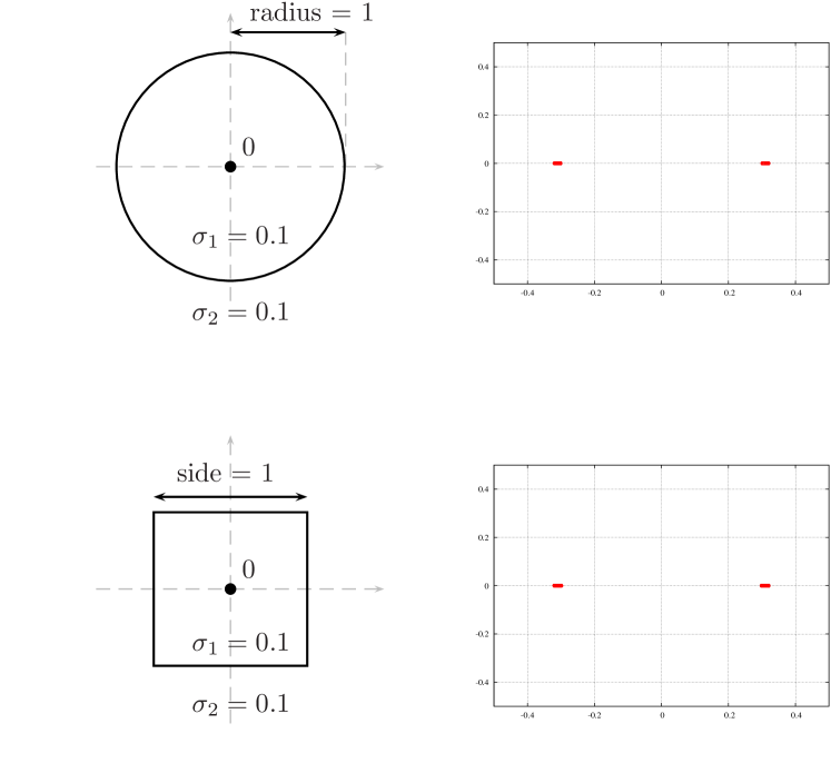
Fig. 2: Spectrum in the case of the unit circle and the square: same $\sigma_{j}$

a numerical approximation of the spectrum of $\mathbb{J}_{2}$ obtained from a boundary element discretization of the Calderón projectors $\mathbb{P}_{1,2}$ using $P_{1}$-Lagrange shape functions for two different geometries: $\Gamma$ either a unit circle or a unit square. We took $a=1$ and $\sigma_{1}=\sigma_{2}=0.1$ so that the exact spectrum of $\mathbb{J}_{2}$ given in (59) is approximately at $\{\pm 0.301511\}$ (up to 6 digits accuracy). We observe that the spectrum of the numerical approximation in Figure 2 clusters around the theoretical values $\pm 0.301511$, but is not exactly a point spectrum, which is due to discretization and quadrature errors of the integral operators. We also see that the numerical spectrum appears to depend only very weakly on the geometry.

Next we consider the same computation as before with the square shaped geometry, but in the case where the sigmas are different, $\sigma_{1}=-0.4$ and $\sigma_{2}=1$. We show in Figure 3

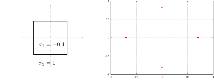
Fig. 3: Spectrum in the case of the square geometry: different $\sigma_{j}$

the corresponding spectrum of the Jacobi iteration operator. We clearly see that this spectrum has four clusters associated with the two pairs of opposite eigenvalues.

Finally, we consider the same experiment as above, but in the case where the material constant $a$ is different in the two subdomains, $a_{1}=1$ in $\Omega_{1}$ and $a_{2}=5$ in $\Omega_{2}$. This contrast of material characteristics only induces compact perturbations of the integral operators, so the accumulation points of the spectrum of the Jacobi iteration are preserved, as one can see in Figure 4.

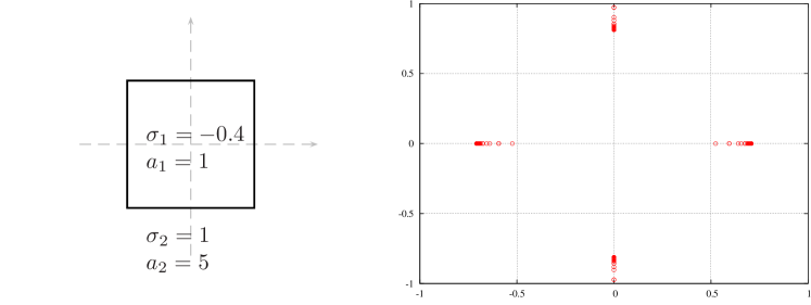
Fig. 4: Spectrum in the case of the square with different $\sigma_{j}$ and varying coefficient $a$

4.4 Multitrace Formulation with 3 Subdomains

We examine now a situation similar to Subsection 2.4 in a higher dimensional context. We consider three Lipschitz domains with bounded boundaries $\Omega_{j},j=0,1,2$ such that $\Omega_{j}\cap\Omega_{k}=\emptyset$ for $j\neq k$ and $\mathbb{R}^{d}=\overline{\Omega}_{0}\cup\overline{\Omega}_{1}\cup\overline{\Omega}_{2}$. To fix ideas, we assume that $\Omega_{0}$ and $\Omega_{1}$ are bounded, and $\partial\Omega_{0}=\partial\Omega_{1}\cup\partial\Omega_{2}$ and $\partial\Omega_{1}\cap\partial\Omega_{2}=\emptyset$, for an example, see Figure 5.

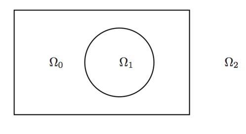
Fig. 5: Example of a decomposition into three subdomains

Let $\Gamma_{1}:=\partial\Omega_{0}\cap\partial\Omega_{1}$ and $\Gamma_{2}:=\partial\Omega_{0}\cap\partial\Omega_{2}$. For given $h^{j}_{\mathrm{D}}\in\mathrm{H}^{1/2}(\Gamma_{j})$ and $h^{j}_{\mathrm{N}}\in\mathrm{H}^{-1/2}(\Gamma_{j})$, we are interested in solving a transmission problem of the form

$$\left\{\begin{array}[]{l}u\in\mathrm{H}^{1}(\mathbb{R}^{d}\setminus(\Gamma_{1}\cup\Gamma_{2})),\\ -\Delta u+a^{2}u=0\quad\textrm{in}\;\;\Omega_{j},\\ [u]_{\Gamma_{j}}=h_{\mathrm{D}}^{j},\quad[\partial_{n}u]_{\Gamma_{j}}=h_{\mathrm{N}}^{j},\quad\quad j=0,1,2,\end{array}\right.$$ (60)

where by denoting $u_{j}=u|_{\Omega_{j}}$, we set $[u]_{\Gamma_{j}}:=u_{j}|_{\Gamma_{j}}-u_{0}|_{\Gamma_{j}}$ for $j=1,2$, and $[\partial_{n}u]_{\Gamma_{j}}:=\boldsymbol{n}_{j}\cdot\nabla u_{j}|_{\Gamma_{j}}+\boldsymbol{n}_{0}\cdot\nabla u_{0}|_{\Gamma_{j}}$, $j=1,2$.

We rewrite this problem by means of a local multitrace formulation. In what follows we denote by $T_{j}$, $j=0,1,2$ the trace operator (52) associated to each subdomain $\Omega_{j}$, and denote the traces by $U_{j}:=T_{j}(u)$. We set $U_{0,j}:=U_{0}|_{\Gamma_{j}}$. We denote by $G_{j}$ the potential operator (51) associated to each $\Omega_{j}$, and $\mathbb{P}_{j}$ is the corresponding Calderón projector.

Observe that, since we have the decomposition $\partial\Omega_{0}=\partial\Omega_{1}\cup\partial\Omega_{2}$, the Calderón projector $\mathbb{P}_{0}$ can be expanded into a $2\times 2$ matrix of integral operators,

$$\mathbb{P}_{0}=\left[\begin{array}[]{cc}\widetilde{\mathbb{P}}_{1,1}&\mathbb{R}_{1,2}\\ \mathbb{R}_{2,1}&\widetilde{\mathbb{P}}_{2,2}\end{array}\right].$$ (61)

A close inspection of the definition of the Calderón projector shows that $\mathbb{R}_{1,2}=-X\cdot(T_{1}\cdot G_{2})\cdot X$ and similarly $\mathbb{R}_{2,1}=-X\cdot(T_{2}\cdot G_{1})\cdot X$. Take any element $V\in\mathrm{H}^{1/2}(\Gamma_{1})\times\mathrm{H}^{-1/2}(\Gamma_{1})$ and set $v(\boldsymbol{x}):=G_{1}(XV)(\boldsymbol{x})$. This function satisfies in particular $-\Delta v+a^{2}v=0$ in $\Omega_{2}$, which means that $G_{2}(T_{2}v)(\boldsymbol{x})=0$ for $\boldsymbol{x}\in\Omega_{1}$ according to Proposition 2. In particular $T_{1}G_{2}(T_{2}v)=0$. From this we conclude that

$$\begin{array}[]{ll}\mathbb{R}_{1,2}\cdot\mathbb{R}_{2,1}(V)&=(\,X\cdot(T_{1}\cdot G_{2})\cdot X\,)\cdot(\,X\cdot(T_{2}\cdot G_{1})\cdot X\,)(V)\\[5.0pt] &=X(T_{1}\cdot G_{2})\cdot(T_{2}\cdot G_{1})X(V)\\[5.0pt] &=X\cdot T_{1}\cdot G_{2}(T_{2}v)=0.\end{array}$$

We prove in a similar manner that $\mathbb{R}_{2,1}\cdot\mathbb{R}_{1,2}(V)=0$ for any $V\in\mathrm{H}^{1/2}(\Gamma_{2})\times\mathrm{H}^{-1/2}(\Gamma_{2})$. Since, in the above arguments, $V$ was chosen arbitrarily, we conclude that

$$\mathbb{R}_{2,1}\cdot\mathbb{R}_{1,2}=0,\quad\textrm{and}\quad\mathbb{R}_{1,2}\cdot\mathbb{R}_{2,1}=0.$$

Other remarkable identities involving $\mathbb{R}_{2,1},\mathbb{R}_{1,2}$ can be derived. Indeed for any $V\in\mathrm{H}^{1/2}(\Gamma_{1})\times\mathrm{H}^{-1/2}(\Gamma_{1})$, the function $v(\boldsymbol{x}):=G_{1}(XV)(\boldsymbol{x})$ satisfies $-\Delta v+a^{2}v=0$ in $\Omega_{2}$, so $G_{2}(T_{2}v)(\boldsymbol{x})=v(\boldsymbol{x})$ for $\boldsymbol{x}\in\Omega_{2}$ according to Proposition 2 and, consequently, $\mathbb{P}_{2}T_{2}(v)=T_{2}(v)$ which leads to $\mathbb{P}_{2}X\mathbb{R}_{2,1}V=X\mathbb{R}_{2,1}V$. We prove similarly $\mathbb{P}_{1}X\mathbb{R}_{1,2}V=X\mathbb{R}_{1,2}V$ for any $V\in\mathrm{H}^{1/2}(\Gamma_{2})\times\mathrm{H}^{-1/2}(\Gamma_{2})$. Since, in this argumentation, the $V$’s were chosen arbitrarily we conclude that

$$\mathbb{P}_{1}X\mathbb{R}_{1,2}=X\mathbb{R}_{1,2},\quad\textrm{and}\quad\mathbb{P}_{2}X\mathbb{R}_{2,1}=X\mathbb{R}_{2,1}.$$

We prove in a similar manner that $\mathbb{R}_{1,2}\widetilde{\mathbb{P}}_{2}=\mathbb{R}_{1,2}$ and $\mathbb{R}_{2,1}\widetilde{\mathbb{P}}_{1}=\mathbb{R}_{2,1}$. For the diagonal blocks of (61), we prove in a similar manner as in (54) that

$$X\mathbb{P}_{j}X=\operatorname{I}-\widetilde{\mathbb{P}}_{j}.$$

In particular the $\widetilde{\mathbb{P}}_{j}$ are projectors. Given three relaxation parameters $\sigma_{j}$, $j=0,1,2$, the local multitrace formulation of Problem (60) is again of the same form here as in the simple one dimensional case (28), and we obtain in matrix form

$$\left[\begin{array}[]{cccc}(1+\sigma_{1})\operatorname{I}-\mathbb{P}_{1}&-\sigma_{1}X&0&0\\ -\sigma_{0}X&(1+\sigma_{0})\operatorname{I}-\widetilde{\mathbb{P}}_{1}&-\mathbb{R}_{2,1}&0\\ 0&-\mathbb{R}_{1,2}&(1+\sigma_{0})\operatorname{I}-\widetilde{\mathbb{P}}_{2}&-\sigma_{0}X\\ 0&0&-\sigma_{2}X&(1+\sigma_{2})\operatorname{I}-\mathbb{P}_{2}\end{array}\right]\left[\begin{array}[]{c}U_{1}\\ U_{0,1}\\ U_{0,2}\\ U_{2}\end{array}\right]=F,$$

where $F$ is the right hand side taking into account the data $h_{\mathrm{D}}^{j},h_{\mathrm{N}}^{j}$, $j=1,2$, as we have shown in the simple 1D case. To simplify notations, we set $\alpha_{j}:=\sigma_{j}^{-1}(1+\sigma_{j})^{-1}$, so that $\alpha_{j}(\sigma_{j}\operatorname{I}+\mathbb{P}_{j})\cdot((1+\sigma_{j})\operatorname{I}-\mathbb{P}_{j})=\operatorname{I}$. The Jacobi iteration matrix associated to the multitrace formulation then becomes

$$\begin{array}[]{c}\mathbb{J}_{3}=\left[\begin{array}[]{cccc}\alpha_{1}(\sigma_{1}\operatorname{I}+\mathbb{P}_{1})&0&0&0\\ 0&\alpha_{0}(\sigma_{0}\operatorname{I}+\widetilde{\mathbb{P}}_{1})&\alpha_{0}\mathbb{R}_{1,2}&0\\ 0&\alpha_{0}\mathbb{R}_{2,1}&\alpha_{0}(\sigma_{0}\operatorname{I}+\widetilde{\mathbb{P}}_{2})&0\\ 0&0&0&\alpha_{2}(\sigma_{2}\operatorname{I}+\mathbb{P}_{2})\end{array}\right]\\ \cdot\left[\begin{array}[]{cccc}0&\sigma_{1}X&0&0\\ \sigma_{0}X&0&0&0\\ 0&0&0&\sigma_{0}X\\ 0&0&\sigma_{2}X&0\end{array}\right].\end{array}$$ (62)

For the sake of simplicity, to examine the spectrum of the Jacobi operator $\mathbb{J}_{3}$, we restrict our analysis to the case where

$$\sigma_{0}=\sigma_{1}=\sigma_{2}:=\sigma\quad\Longrightarrow\quad\alpha_{0}=\alpha_{1}=\alpha_{2}=:\alpha.$$

Under this hypothesis, we can clearly factorize $\alpha\sigma=(1+\sigma)^{-1}$ in (62) so it suffices to examine the spectrum of $(1+\sigma)\mathbb{J}_{3}$. As in Subsection 4.3, we study the square of this operator. Tedious, but straightforward calculations then yield

$$\begin{array}[]{r}(1+\sigma)^{2}(\mathbb{J}_{3})^{2}=\left[\begin{array}[]{cccc}(\sigma\operatorname{I}+\mathbb{P}_{1})&0&0&0\\ 0&(\sigma\operatorname{I}+\widetilde{\mathbb{P}}_{1})&\mathbb{R}_{1,2}&0\\ 0&\mathbb{R}_{2,1}&(\sigma\operatorname{I}+\widetilde{\mathbb{P}}_{2})&0\\ 0&0&0&(\sigma\operatorname{I}+\mathbb{P}_{2})\end{array}\right]\\ \cdot\left[\begin{array}[]{cccc}(1+\sigma)\operatorname{I}-\mathbb{P}_{1}&0&0&X\mathbb{R}_{1,2}X\\ 0&(1+\sigma)\operatorname{I}-\widetilde{\mathbb{P}}_{1}&0&0\\ 0&0&(1+\sigma)\operatorname{I}-\widetilde{\mathbb{P}}_{2}&0\\ X\mathbb{R}_{2,1}X&0&0&(1+\sigma)\operatorname{I}-\mathbb{P}_{2}\end{array}\right]\\ =\left[\begin{array}[]{cccc}\sigma(1+\sigma)\operatorname{I}&0&0&(1+\sigma)X\mathbb{R}_{1,2}X\\ 0&\sigma(1+\sigma)\operatorname{I}&\sigma\mathbb{R}_{1,2}&0\\ 0&\sigma\mathbb{R}_{2,1}&\sigma(1+\sigma)\operatorname{I}&0\\ (1+\sigma)X\mathbb{R}_{2,1}X&0&0&\sigma(1+\sigma)\operatorname{I}\end{array}\right].\end{array}$$ (63)

In the course of the above calculations, we used again several remarkable identities: $\mathbb{P}_{2}X\mathbb{R}_{2,1}=X\mathbb{R}_{2,1}$ and $\mathbb{P}_{1}X\mathbb{R}_{1,2}=X\mathbb{R}_{1,2}$ as well as $\mathbb{R}_{2,1}\widetilde{\mathbb{P}}_{1}=\mathbb{R}_{2,1}$ and $\mathbb{R}_{1,2}\widetilde{\mathbb{P}}_{2}=\mathbb{R}_{1,2}$. Now observe that $(1+\sigma)(\mathbb{J}_{3})^{2}-\sigma\operatorname{I}$ only contains extra diagonal terms involving $\mathbb{R}_{1,2}$ and $\mathbb{R}_{2,1}$. Since $\mathbb{R}_{2,1}\mathbb{R}_{1,2}=\mathbb{R}_{1,2}\mathbb{R}_{2,1}=0$, taking the square of this operator yields

$$\Big{(}\;(1+\sigma)\mathbb{J}_{3}^{2}-\sigma\operatorname{I}\;\Big{)}^{2}=\left[\begin{array}[]{cccc}X\mathbb{R}_{1,2}\mathbb{R}_{2,1}X&0&0&0\\ 0&\mathbb{R}_{1,2}\mathbb{R}_{2,1}&0&0\\ 0&0&\mathbb{R}_{2,1}\mathbb{R}_{1,2}&0\\ 0&0&0&X\mathbb{R}_{2,1}\mathbb{R}_{1,2}X\end{array}\right]=0.$$

From this we conclude that the only eigenvalue of $\mathbb{J}_{3}^{2}$ is $\sigma/(1+\sigma)$. This gives very precise information about the spectrum of $\mathbb{J}_{3}$ in the case where all relaxation parameters are equal, i.e.

$$\sigma(\mathbb{J}_{3})\subset\Big{\{}+\sqrt{\frac{\sigma}{1+\sigma}},-\sqrt{\frac{\sigma}{1+\sigma}}\;\Big{\}}.$$ (64)

Considering once again a discretization of the boundary integral operators by Lagrange $P_{1}$ shape functions, we show in Figure 6

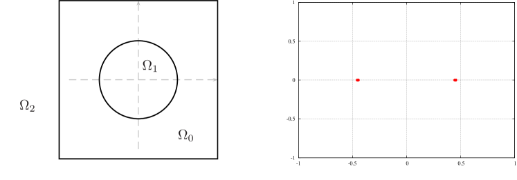
Fig. 6: Spectrum of the Jacobi iteration for $\sigma_{0}=\sigma_{1}=\sigma_{2}=0.25$

the results of a numerical experiment for the geometry shown on the left in Figure 6, which is a configuration with three subdomains. We chose to solve $-\Delta u+a^{2}u=0$ in each subdomain with $a=1$. We represent the spectrum of the Jacobi iteration matrix associated to the local multitrace formulation in Figure 6 on the right, where all relaxation parameters in all subdomains are equal to $\sigma=0.25$. In accordance with (64), we see that eigenvalues cluster around the pair of opposite real values $\pm\sqrt{0.25/1.25}\simeq 0.44721$.

In Figure 7,

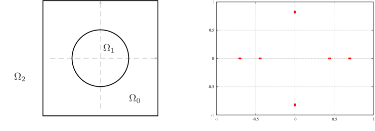
Fig. 7: Spectrum of the Jacobi iteration for $\sigma_{0}=-0.4$, $\sigma_{1}=1$ and $\sigma_{2}=0.25$

we present the spectrum of the Jacobi iterations for a similar numerical experiment except that we considered three different values of the relaxation parameters, taking $\sigma_{0}=-0.4$, $\sigma_{1}=1$, $\sigma_{2}=0.25$. We observe clusters of eigenvalues around the three pairs of opposite values $\pm\sqrt{\sigma_{j}/(1+\sigma_{j})}$ which is consistent with both Subsection 2.4 and (64).

Finally, in Figure 8,

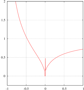
Fig. 8: Spectral radius of the Jacobi iteration versus $\sigma$ in the case where $\sigma_{0}=\sigma_{1}=\sigma_{2}=\sigma$

we consider the case where all relaxation parameters are equal to $\sigma$ and present the spectral radius of the Jacobi iteration versus the value of this relaxation parameter $\sigma$ . We essentially recover the curve presented in Figure 1, which shows that the fundamental convergence properties of the iterative multitrace formulation we studied first on a simple one dimensional model problem remain in this general situation. The additional overshoot we see close to $\sigma=0$ in Figure 8 compared to Figure 1 is due to the numerical difficulty which we explained in the one dimensional case when $\sigma$ approaches zero.

5 Conclusion

We used a simple one dimensional model problem to present a recent multitrace formulation with relaxation parameters without resorting to a functional analysis framework. The simple setting allowed us to study a natural block Jacobi iteration for the multitrace formulation, and to determine the dependence of this iteration on the relaxation parameter. We also determined an optimal choice for the relaxation parameter, and obtained an algorithm with converges in a finite number of steps. This algorithm is related to a well know algorithm that also has this property: the optimal Schwarz method. We then left our simple model problem and showed that the properties we discovered hold also in a much more general higher dimensional setting, and this independently of the geometry of the decomposition. An important open question is the cost of such multitrace formulations and their associated iterative solution. For optimal Schwarz methods it is known that it is more efficient to use approximations of the Dirichlet to Neumann maps to obtain practical algorithms. It is not clear yet how in the multitrace formulation such approximations could be introduced.

References

- [1] X. Claeys. Essential spectrum of local multi-trace boundary integral operators. ArXiv e-prints, Aug. 2015.
- [2] X. Claeys and R. Hiptmair. Electromagnetic scattering at composite objects: a novel multi-trace boundary integral formulation. ESAIM Math. Model. Numer. Anal., 46(6):1421–1445, 2012.
- [3] X. Claeys and R. Hiptmair. Multi-trace boundary integral formulation for acoustic scattering by composite structures. Comm. Pure Appl. Math., 66(8):1163–1201, 2013.
- [4] X. Claeys, R. Hiptmair, and E. Spindler. A second-kind Galerkin boundary element method for scattering at composite objects. Technical Report 2013-13 (revised), Seminar for Applied Mathematics, ETH Zürich, 2013.
- [5] V. Dolean and M. J. Gander. Multitrace formulations and the Dirichlet-Neumann algorithm. In Domain Decomposition Methods in Science and Engineering XXII. Springer LNCSE, 2015.
- [6] B. Engquist and L. Ying. Sweeping preconditioner for the Helmholtz equation: hierarchical matrix representation. Communications on pure and applied mathematics, 64(5):697–735, 2011.
- [7] B. Engquist and L. Ying. Sweeping preconditioner for the Helmholtz equation: moving perfectly matched layers. Multiscale Modeling & Simulation, 9(2):686–710, 2011.
- [8] M. Gander and F. Nataf. AILU: A preconditioner based on the analytic factorization of the elliptic operator. Numer. Linear Algebra Appl., 7:505–526, 2000.
- [9] M. J. Gander. Optimized Schwarz methods. SIAM Journal on Numerical Analysis, 44(2):699–731, 2006.
- [10] M. J. Gander, L. Halpern, and F. Nataf. Optimal convergence for overlapping and non-overlapping Schwarz waveform relaxation. In C.-H. Lai, P. Bjørstad, M. Cross, and O. Widlund, editors, Eleventh international Conference of Domain Decomposition Methods. ddm.org, 1999.
- [11] M. J. Gander, L. Halpern, and F. Nataf. Optimal Schwarz waveform relaxation for the one dimensional wave equation. SIAM Journal on Numerical Analysis, 41(5):1643–1681, 2003.
- [12] M. J. Gander and F. Kwok. Optimal interface conditions for an arbitrary decomposition into subdomains. In Domain Decomposition Methods in Science and Engineering XIX, pages 101–108. Springer, 2011.
- [13] M. J. Gander, S. Loisel, and D. B. Szyld. An optimal block iterative method and preconditioner for banded matrices with applications to PDEs on irregular domains. SIAM Journal on Matrix Analysis and Applications, 33(2):653–680, 2012.
- [14] M. J. Gander and F. Nataf. An incomplete LU preconditioner for problems in acoustics. Journal of Computational Acoustics, 13(03):455–476, 2005.
- [15] R. Hiptmair and C. Jerez-Hanckes. Multiple traces boundary integral formulation for Helmholtz transmission problems. Adv. Comput. Math., 37(1):39–91, 2012.
- [16] R. Hiptmair, C. Jerez-Hanckes, J. Lee, and Z. Peng. Domain decomposition for boundary integral equations via local multi-trace formulations. Technical Report 2013-08 (revised), Seminar for Applied Mathematics, ETH Zürich, 2013.
- [17] W. McLean. Strongly elliptic systems and boundary integral equations. Cambridge University Press, Cambridge, 2000.
- [18] F. Nataf, F. Rogier, and E. de Sturler. Optimal interface conditions for domain decomposition methods. Technical Report 301, CMAP (Ecole Polytechnique), 1994.
- [19] S. Sauter and C. Schwab. Boundary element methods, volume 39 of Springer Series in Computational Mathematics. Springer-Verlag, Berlin, 2011.
- [20] C. Wagner and G. Wittum. Adaptive filtering. Numerische Mathematik, 78(2):305–328, 1997.