Bayesian Lower Bounds for Dense or Sparse (Outlier) Noise in the RMT Framework
Abstract
Robust estimation is an important and timely research subject. In this paper, we investigate performance lower bounds on the mean-square-error (MSE) of any estimator for the Bayesian linear model, corrupted by a noise distributed according to an i.i.d. Student’s t-distribution. This class of prior parametrized by its degree of freedom is relevant to modelize either dense or sparse (accounting for outliers) noise. Using the hierarchical Normal-Gamma representation of the Student’s t-distribution, the Van Trees’ Bayesian Cramér-Rao bound (BCRB) on the amplitude parameters is derived. Furthermore, the random matrix theory (RMT) framework is assumed, i.e., the number of measurements and the number of unknown parameters grow jointly to infinity with an asymptotic finite ratio. Using some powerful results from the RMT, closed-form expressions of the BCRB are derived and studied. Finally, we propose a framework to fairly compare two models corrupted by noises with different degrees of freedom for a fixed common target signal-to-noise ratio (SNR). In particular, we focus our effort on the comparison of the BCRBs associated with two models corrupted by a sparse noise promoting outliers and a dense (Gaussian) noise, respectively.
Index Terms:
Bayesian hierarchical linear model, Bayesian Cramér-Rao bound, sparse outlier noise, dense noise, random matrix theoryI Introduction
In the context of robust data modeling [1], the measurement vector may be corrupted by noise containing outliers. This class of noise is sometimes referred to as sparse noise and is described by a distribution with heavy-tails [2, 3, 4, 5, 6, 7]. Conversely, we usually call dense a noise that does not share this property and the most popular prior is probably Gaussian noise. Depending on the application context, outliers may be identified, e.g., as corrupted information or incomplete data [8].
A robust and relevant noise prior which is able to take into account outliers is the Student’s t-distribution with low degrees of freedom [9, 10, 11, 12]. In addition, dense noise can also be encompassed thanks to the Student’s t-distribution prior for an infinite degree of freedom. A convenient framework to deal with a wide class of distributions is well known under the name of hierarchical Bayesian modeling. The Bayesian hierarchical linear model (BHLM) with hierarchical noise prior is used in a wide range of applications, including fusion [13], anomaly detection of hyperspectral images [5], channel estimation [14], blind deconvolution [15], segmentation of astronomical times series [16], etc.
In this work, we adopt such hierarchical prior framework due to its flexibility and ability to modelize a wide class of priors. More precisely, the noise vector is assumed to follow a circular i.i.d. centered Gaussian prior with a variance defined by the inverse of an unknown random hyper-parameter. In addition, if this hyper-parameter is Gamma distributed [17, 18], then the marginalized joint pdf over the hyper-parameter is the Student’s t-distribution.
The Van Trees’ Bayesian Cramér-Rao bound () [19] is a standard and fundamental lower bound on the mean-square-error () of any estimator. The aim of this work is to derive and analyze the of the amplitude parameters for the considered noise prior and using some powerful results from the random matrix theory (RMT) framework [20, 21, 22]. Regarding reference [23], the proposed work is original in the sense that the noise prior is different and the asymptotic regime is assumed. Finally, note that reference [24] tackles a similar problem but does not assume the asymptotic context.
We use the following notation. Scalars, vectors and matrices are denoted by italic lower-case, boldface lower-case and boldface upper-case symbols, respectively. The symbol stands for the trace operator. The identity matrix is denoted by and is the vector filled with zeros. The probability density function (pdf) of a given random variable is denoted by . The symbol refers to the Gaussian distribution, parametrized by its mean and covariance matrix, is the Gamma distribution, described by its shape and rate (inverse scale) parameters, while is the inverse-Gamma distribution. If we have then , where is the Gamma function. And if , then . The non-standardized Student’s t-distribution is defined by three parameters, through the pdf such that As regards the bivariate Normal-Gamma distribution, if we have , then . Finally, the symbol denotes almost sure convergence, is the big notation, is the -th eigenvalue of the considered matrix and the symbol refers to the expectation with respect to .
II Bayesian linear model corrupted by noise outliers
II-A Definition of the random model
Let be the vector of measurements. The BHLM is defined by
| (1) |
where each element of the matrix , with , is drawn from an i.i.d. as a single realization of a sub-Gaussian distribution with zero-mean and variance [25, 22]. The unknown amplitude vector is given by
| (2) |
where is the known amplitude variance. In addition, the measurements are contaminated by a noise vector which is assumed statistically independent from .
II-B Hierarchical Normal-Gamma representation
The -th noise sample is assumed to be circular centered i.i.d. Gaussian according to
| (3) |
where is usually called the noise precision, is an unknown hyper-parameter and is a fixed scale parameter.
If the hyper-parameter is Gamma distributed according to
| (4) |
where is the number of degrees of freedom, the joint distribution of follows a Normal-Gamma distribution [26] such as
| (5) |
The marginal distribution of the joint pdf over the hyper-parameter leads to a non-standardized Student’s t-distribution, given by [27, 11]
| (6) |
such that .
III for Student’s t-distribution
The vector of unknown parameters, denoted by , encompasses the amplitude vector and the noise hyper-parameter, i.e.,
| (8) |
Given an independence assumption between and , the joint pdf can be decomposed as
| (9) |
Let us note an estimator of the unknown vector . Then, the mean square error (), directly linked to the error covariance matrix, verifies the following inequality
| (10) |
where is the matrix defined as the inverse of the Bayesian Information Matrix (BIM) . We can show that the BIM has a block-diagonal structure due to the independence between parameters. Thus, we write
| (11) |
We assume an identifiable BHLM model so that, under weak regularity conditions [19], the BIM is given by
| (12) |
in which
| (13) |
| (14) |
| (15) |
for , and where is the Fisher Information Matrix (FIM) on , is the prior part of the BIM and is the hyper-prior part.
Correspondingly, we have
| (16) |
Conditionally to , the observation vector has the following Gaussian distribution
| (17) |
where and . In what follows, we directly make use of the Slepian-Bangs formula [29, p. 378]
| (18) |
This leads to
| (19) |
Using the fact that , we obtain
| (20) |
According to (2) and considering independent amplitudes, we have
| (21) |
Consequently,
| (22) |
The BIM is therefore composed of the following terms:
| (23) |
| (24) |
The hyper-prior part of the BIM is given by
| (25) |
The second-order moment of an inverse-Gamma distributed random variable is given by
| (26) |
where . This finally leads to
| (27) |
Inverting the BIM, we obtain the for the amplitude parameters
| (28) |
where with (signal-to-noise ratio).
IV in the asymptotic framework
IV-A RMT framework
In this section, we consider the context of large random matrices, i.e., for with . The derived in this context is the asymptotic normalized defined by
| (29) |
IV-B Limit analytical expressions
-
•
For , i.e., , after some manipulations and discarding the terms of order superior or equal to , we obtain
(31) Therefore, an asymptotic analytical expression of the , in the RMT framework, is given by
(32) - •
- •
IV-C Comparison between two models with a target common
We consider two different models:
| (37) | ||||
| (38) |
Model is the reference model and model is the alternative one. According to (30), the asymptotic normalized for the -th model with is defined by
| (39) |
where with . A fair methodology to compare the bounds and is to impose a common target for the models and , i.e., . A simple derivation shows that to reach the target , we must have . Specifically, the corresponding are the following ones:
| (40) | ||||
| (41) |
IV-D Numerical simulations
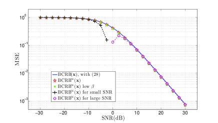
In the following simulations, we consider and so that . The amplitude variance is fixed to . In Fig. 1, we plot the of the amplitude vector , as defined by equations (28) and (30) (asymptotic expression), (32) (small ), (• ‣ IV-B) (small ) and (• ‣ IV-B) (large ), as a function of the in dB for .
We notice that coincides precisely with its asymptotic expression in (30). Thus, the RMT framework predicts precisely the behavior of the of the amplitude as with and allows us to obtain a closed-form expression. Such limit remains correct even for values of and that are relatively not quite large. The expression of the obtained with (32) is a good approximation since here, we have . Finally, we notice that the curves obtained for low and high approximate very well the of the amplitude, asymptotically.
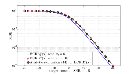
In Fig. 2, as exposed in section IV-C, we consider two different models, with a different value for the number of degrees of freedom . We notice that a lower performance bound is achieved with , especially in the low noise regime, than with . Furthermore, the approximation in (42) is correct, since has a large value. A low value for the number of degrees of freedom is well-adapted for the modelization of sparse (outlier) noise, characterized by a heavy-tailed distribution [31, 32]. This large level in heavy-tailedness leads to robustness [33, 34, 1] while a Gaussian noise model (large degree of freedom) corresponds to a dense noise type. Thus, we can hope to achieve better estimation performances if we consider a model, which promotes sparsity and the presence of outliers in data.
V Conclusion
This work discusses fundamental Bayesian lower bounds for multi-parameter robust estimation. More precisely, we consider a Bayesian linear model corrupted by a sparse noise following a Student’s t-distribution. This class of prior can efficiently modelize outliers. Using the hierarchical Normal-Gamma representation of the Student’s t-distribution, the Van Trees’ Bayesian lower bound () is derived for unknown amplitude parameters in an asymptotic context. By asymptotic, it means that the number of measurements and the number of unknown parameters grow to infinity at a finite rate. Consequently, closed-form expressions of the are obtained using some powerful results from the large random matrix theory. Finally, a framework is provided to fairly compare two models corrupted by noises with different degrees of freedom for a fixed common target . We recall that a small degree of freedom promotes outliers in the sense that the noise prior has heavy-tails. For the amplitude, a lower performance bound is achieved when the number of degrees of freedom is small.
References
- [1] A. M. Zoubir, V. Koivunen, Y. Chakhchoukh, and M. Muma, “Robust estimation in signal processing: A tutorial-style treatment of fundamental concepts,” IEEE Signal Processing Magazine, vol. 29, no. 4, pp. 61–80, 2012.
- [2] K. Mitra, A. Veeraraghavan, and R. Chellappa, “Robust RVM regression using sparse outlier model,” in IEEE Conference on Computer Vision and Pattern Recognition (CVPR), San Francisco, CA, 2010, pp. 1887–1894.
- [3] ——, “Robust regression using sparse learning for high dimensional parameter estimation problems,” in IEEE Int. Conf. Acoust., Speech and Signal Processing (ICASSP), Dallas, TX, 2010, pp. 3846–3849.
- [4] P. Zhuang, W. Wang, D. Zeng, and X. Ding, “Robust mixed noise removal with non-parametric Bayesian sparse outlier model,” in 16th International Workshop on Multimedia Signal Processing (MMSP), Jakarta, Indonesia, 2014, pp. 1–5.
- [5] G. E. Newstadt, A. O. Hero, and J. Simmons, “Robust spectral unmixing for anomaly detection.” in IEEE Workshop on Statistical Signal Processing (SSP), Gold Coast, VIC, 2014, pp. 109–112.
- [6] M. Sundin, S. Chatterjee, and M. Jansson, “Combined modeling of sparse and dense noise improves Bayesian RVM,” in 22nd European Signal Processing Conference (EUSIPCO), Lisbon, Portugal, 2014, pp. 1841–1845.
- [7] ——, “Bayesian learning for robust Principal Component Analysis,” in 23rd European Signal Processing Conference (EUSIPCO), Nice, France, 2015, pp. 2361–2365.
- [8] J. Luttinen, A. Ilin, and J. Karhunen, “Bayesian robust PCA of incomplete data,” Neural Processing Letters, vol. 36, no. 2, pp. 189–202, 2012.
- [9] D. Peel and G. J. McLachlan, “Robust mixture modelling using the t distribution,” Statistics and computing, vol. 10, no. 4, pp. 339–348, 2000.
- [10] S. Kotz and S. Nadarajah, Multivariate t-distributions and their applications. Cambridge University Press, 2004.
- [11] J. Christmas, “Bayesian spectral analysis with Student-t noise,” IEEE Transactions on Signal Processing, vol. 62, no. 11, pp. 2871–2878, 2014.
- [12] H. Zhang, Q. M. J. Wu, T. M. Nguyen, and X. Sun, “Synthetic aperture radar image segmentation by modified Student’s t-mixture model,” IEEE Transactions on Geoscience and Remote Sensing, vol. 52, no. 7, pp. 4391–4403, 2014.
- [13] Q. Wei, N. Dobigeon, and J.-Y. Tourneret, “Bayesian fusion of hyperspectral and multispectral images,” in IEEE Int. Conf. on Acoust., Speech and Signal Processing (ICASSP), Florence, Italy, 2014, pp. 3176–3180.
- [14] N. L. Pedersen, C. N. Manchón, D. Shutin, and B. H. Fleury, “Application of Bayesian hierarchical prior modeling to sparse channel estimation,” in IEEE International Conference on Communications (ICC), Ottawa, ON, 2012, pp. 3487–3492.
- [15] G. Kail, J.-Y. Tourneret, F. Hlawatsch, and N. Dobigeon, “Blind deconvolution of sparse pulse sequences under a minimum distance constraint: A partially collapsed Gibbs sampler method,” IEEE Transactions on Signal Processing, vol. 60, no. 6, pp. 2727–2743, 2012.
- [16] N. Dobigeon, J.-Y. Tourneret, and J. D. Scargle, “Joint segmentation of multivariate astronomical time series: Bayesian sampling with a hierarchical model,” IEEE Transactions on Signal Processing, vol. 55, no. 2, pp. 414–423, 2007.
- [17] A. Gelman, “Prior distributions for variance parameters in hierarchical models (comment on article by Browne and Draper),” Bayesian Analysis, vol. 1, no. 3, pp. 515–534, 2006.
- [18] J. Dahlin, F. Lindsten, T. B. Schön, and A. Wills, “Hierarchical Bayesian ARX models for robust inference,” in 16th IFAC Symposium on System Identification (SYSID), Brussels, Belgium, 2012, pp. 131–136.
- [19] H. L. Van Trees and K. L. Bell, Bayesian bounds for parameter estimation and nonlinear filtering/tracking. New York: Wiley-IEEE Press, 2007.
- [20] J. W. Silverstein and Z. Bai, “On the empirical distribution of eigenvalues of a class of large dimensional random matrices,” Journal of Multivariate analysis, vol. 54, no. 2, pp. 175–192, 1995.
- [21] A. M. Tulino and S. Verdú, Random matrix theory and wireless communications. Foundations and Trends in Communications and Information Theory. Now Publishers Inc., 2004, vol. 1, no. 1.
- [22] R. Couillet and M. Debbah, Random matrix methods for wireless communications. Cambridge University Press, 2011.
- [23] M. N. El Korso, R. Boyer, P. Larzabal, and B.-H. Fleury, “Estimation performance for the Bayesian hierarchical linear model,” IEEE Signal Processing Letters, vol. 23, no. 4, pp. 488–492, 2016.
- [24] R. Prasad and C. R. Murthy, “Cramér-Rao-type bounds for sparse Bayesian learning,” IEEE Transactions on Signal Processing, vol. 61, no. 3, pp. 622–632, 2013.
- [25] V. V. Buldygin and Y. V. Kozachenko, Metric characterization of random variables and random processes. American Mathematical Soc., 2000, vol. 188.
- [26] J. M. Bernardo and A. F. M. Smith, Bayesian theory. New York: J. Wiley, 1994.
- [27] M. Svensén and C. M. Bishop, “Robust Bayesian mixture modelling,” Neurocomputing, vol. 64, pp. 235–252, 2005.
- [28] G. Sfikas, C. Nikou, and N. Galatsanos, “Robust image segmentation with mixtures of Student’s t-distributions,” in International Conference on Image Processing (ICIP), vol. 1, Sant Antonio, TX, 2007, pp. I–273 – I–276.
- [29] P. Stoica and R. L. Moses, Spectral analysis of signals. Pearson Prentice Hall, Upper Saddle River, NJ, 2005.
- [30] G. B. Arfken and H. J. Weber, Mathematical methods for physicists, sixth edition. Academic press, 2005.
- [31] G. Tzagkarakis and P. Tsakalides, “Bayesian compressed sensing of a highly impulsive signal in heavy-tailed noise using a multivariate Cauchy prior,” in 17th European Signal Processing Conference, Glasgow, Scotland, 2009, pp. 2293–2297.
- [32] A. Amini, M. Unser, and F. Marvasti, “Compressibility of deterministic and random infinite sequences,” IEEE Transactions on Signal Processing, vol. 59, no. 11, pp. 5193–5201, 2011.
- [33] K. L. Lange, R. J. A. Little, and J. M. G. Taylor, “Robust statistical modeling using the t distribution,” Journal of the American Statistical Association, vol. 84, no. 408, pp. 881–896, 1989.
- [34] N. Delannay, C. Archambeau, and M. Verleysen, “Improving the robustness to outliers of mixtures of probabilistic PCAs,” Advances in Knowledge Discovery and Data Mining, vol. 5012, pp. 527–535, 2008.