Spectral analysis of the Navier-Stokes equations using the combination matrix

Lawrence C. Cheung and Tamer Zaki

April 2016

1 Introduction

This work is a continuation of the analysis first presented in Cheung & Zaki (2014). In that study, the combination matrix was introduced as a means to tractably handle the nonlinear terms in the spectral domain. An energy equation was derived from the Navier-Stokes and applied to homongenous isotropic turbulence, yielding Kolmogorov’s -5/3 scaling in the inertial range.

In this document, a different approach is discussed. Rather than analyze solutions to the energy equation, we examine the forced Navier-Stokes equations in spectral space and determine if direct solutions to the momentum equations can be found. This is done by using the combination matrix to rewrite the Navier-Stokes as a system of intersecting quadratic polynomials. Intrepreted geometrically, any solution to the Navier-Stokes can be represented as a the intersection of a multiple conic sections. Using the Chebyshev basis, a similar formulation for wall-bounded channel flow can also be found.

We then find that the tools of commutative algebra can be applied to determine the solvability of such nonlinear systems. Furthermore, through the use of polynomial resultants and Groebner bases, all possible solutions to the systems can be found. This processes is demonstrated on a simple nonlinear ODE, although it can be extended to more complicated applications.

2 Mathematical formulation

2.1 Homogeneous turbulence

Here we consider the governing Navier-Stokes equations for the fluid velocity $\mathbf{u}(\mathbf{x},t)$, pressure $\mathbf{p}(\mathbf{x},t)$, given a uniform fluid of density $\rho$, viscosity $\nu$, and body force $\mathbf{f}(\mathbf{x},t)$.

$$\boldsymbol{\nabla}\cdot\mathbf{u}=0$$ (2.1a)

$$\frac{\partial\mathbf{u}}{\partial t}+\mathbf{u}\cdot\boldsymbol{\nabla}\mathbf{u}+\frac{1}{\rho}\nabla p-\nu\nabla^{2}\mathbf{u}+\mathbf{f}=0$$ (2.1b)

For the sake of algebraic simplicity later on, we assume that the body force $\mathbf{f}$ is divergence free: $\nabla\cdot\mathbf{f}=0$. However, the analysis can also be repeated for the general case of arbitrary $\mathbf{f}$ without significant modification. For the pressure field, velocity fields, and body forces we express them in terms of a Fourier expansion:

$$\mathbf{u}(\mathbf{x},t)=\sum_{\mathbf{k}}\hat{\mathbf{u}}^{\mathbf{k}}e^{ik_{0}t}e^{ik_{1}x_{1}+ik_{2}x_{2}+ik_{3}x_{3}},$$ (2.2a)

$$p(\mathbf{x},t)=\sum_{\mathbf{k}}\hat{p}^{\mathbf{k}}e^{ik_{0}t}e^{ik_{1}x_{1}+ik_{2}x_{2}+ik_{3}x_{3}}.$$ (2.2b)

$$\mathbf{f}(\mathbf{x},t)=\sum_{\mathbf{k}}\hat{\mathbf{f}}^{\mathbf{k}}e^{ik_{0}t}e^{ik_{1}x_{1}+ik_{2}x_{2}+ik_{3}x_{3}},$$ (2.2c)

The notation used here is similar to the notation used in Cheung & Zaki (2014). The superscript on the Fourier coefficient $\hat{a}_{i}^{\mathbf{k}}$ refers to the wavenumber $\mathbf{k}$, while the subscript refers to the spatial index $i=1,2,3$ of the variable. Note, however, that the wavenumber $\mathbf{k}$ in this context has four components: $\mathbf{k}=\left(k_{0},k_{1},k_{2},k_{3}\right)$, where $k_{0}$ is the temporal frequency and is synonymous with the frequency $\omega$. However, please note that we define $k^{2}=k_{1}^{2}+k_{2}^{2}+k_{3}^{2}$, and summations over the spatial coordinates are taken to be over $i,j=1,2,3$ only. Furthermore, the summation convention is not adopted throughout this analysis in order to avoid any confusion.

To analyze the nonlinear terms, we introduce the combination matrix $C^{\mathbf{pq},\mathbf{k}}$, which is defined as

$$C^{\mathbf{pq,k}}=\begin{cases}0,&\mathbf{p}+\mathbf{q}\neq\mathbf{k}\\ 1,&\mathbf{p}+\mathbf{q}=\mathbf{k}\end{cases}.$$ (2.3)

Using this definition, we can easily represent the multiplication of two functions $f(\mathbf{x})$ and $g(\mathbf{x})$ in spectral space. For instance, if $h(\mathbf{x})=f(\mathbf{x})g(\mathbf{x})$ and the functions can be written in terms of the Fourier expansions

$$h(\mathbf{x})=\sum_{\mathbf{k}}\hat{h}^{\mathbf{k}}e^{i\mathbf{k}\cdot\mathbf{x}}\qquad f(\mathbf{x})=\sum_{\mathbf{p}}\hat{f}^{\mathbf{p}}e^{i\mathbf{p}\cdot\mathbf{x}}\qquad g(\mathbf{x})=\sum_{\mathbf{q}}\hat{g}^{\mathbf{q}}e^{i\mathbf{q}\cdot\mathbf{x}}$$

then the combination matrix allows us to express the convolution in terms of a bilinear product, i.e.,

$$\hat{h}^{\mathbf{k}}=\sum_{\mathbf{p}}\sum_{\mathbf{q}}\hat{f}^{\mathbf{p}}C^{\mathbf{pq,k}}\hat{g}^{\mathbf{q}}.$$ (2.4)

As discussed in Cheung & Zaki (2014), this treatment allows the nonlinear terms of the Navier-Stokes to represented in a tractable manner. For instance, the nonlinear convective term for the wavenumber $\mathbf{k}$ can be expressed in spectral space as

$$\left(\mathbf{u}\cdot\boldsymbol{\nabla}\mathbf{u}\right)^{\mathbf{k}}=i\sum_{\mathbf{p,q}}\left(\begin{array}[]{c}\left(\hat{u}_{1}^{\mathbf{p}}q_{1}C^{\mathbf{pq,k}}\hat{u}_{1}^{\mathbf{q}}+\hat{u}_{2}^{\mathbf{p}}q_{2}C^{\mathbf{pq,k}}\hat{u}_{1}^{\mathbf{q}}+\hat{u}_{3}^{\mathbf{p}}q_{3}C^{\mathbf{pq,k}}\hat{u}_{1}^{\mathbf{q}}\right)\\ \left(\hat{u}_{1}^{\mathbf{p}}q_{1}C^{\mathbf{pq,k}}\hat{u}_{2}^{\mathbf{q}}+\hat{u}_{2}^{\mathbf{p}}q_{2}C^{\mathbf{pq,k}}\hat{u}_{2}^{\mathbf{q}}+\hat{u}_{3}^{\mathbf{p}}q_{3}C^{\mathbf{pq,k}}\hat{u}_{2}^{\mathbf{q}}\right)\\ \left(\hat{u}_{1}^{\mathbf{p}}q_{1}C^{\mathbf{pq,k}}\hat{u}_{3}^{\mathbf{q}}+\hat{u}_{2}^{\mathbf{p}}q_{2}C^{\mathbf{pq,k}}\hat{u}_{3}^{\mathbf{q}}+\hat{u}_{3}^{\mathbf{p}}q_{3}C^{\mathbf{pq,k}}\hat{u}_{3}^{\mathbf{q}}\right)\end{array}\right).$$ (2.5)

If we define the matrix $\boldsymbol{\Gamma}_{ij,m}^{\mathbf{pq},\mathbf{k}}$ as

$$\boldsymbol{\Gamma}_{ij,m}^{\mathbf{pq},\mathbf{k}}=\left(\begin{array}[]{ccc}0&0&q_{1}C^{\mathbf{pq},\mathbf{k}}\\ 0&0&q_{2}C^{\mathbf{pq},\mathbf{k}}\\ 0&0&q_{3}C^{\mathbf{pq},\mathbf{k}}\end{array}\right)\left(\begin{array}[]{ccc}0&\mathbf{I}&0\\ 0&0&\mathbf{I}\\ \mathbf{I}&0&0\end{array}\right)^{(m)}$$ (2.6)

where the matrix powers $m=1,2,3$ and $\mathbf{I}\equiv\delta^{\mathbf{pq}}$ is the infinite identity matrix, then we can compactly represent the entire nonlinear convective term as

$$(\mathbf{u}\cdot\nabla\mathbf{u})_{m}^{\mathbf{k}}=i\sum_{\mathbf{p,q}}\sum_{i,j}\hat{u}_{i}^{\mathbf{p}}\boldsymbol{\Gamma}_{ij,m}^{\mathbf{pq,k}}\hat{u}_{j}^{\mathbf{q}}.$$ (2.7)

By taking the divergence of (2.1b) and invoking the continuity constraint, the pressure Poisson equation $\nabla^{2}p=-\rho\boldsymbol{\nabla\cdot}\left(\mathbf{u}\cdot\boldsymbol{\nabla}\mathbf{u}\right)$ is obtained. Inserting (2.2a), and using (2.3) in this equation produces the equivalent form in spectral space:

$$\hat{p}^{\mathbf{k}}=\frac{\rho}{k^{2}}\sum_{i,j}\sum_{\mathbf{p},\mathbf{q}}(p_{i}q_{j})\left(\hat{u}_{j}^{\mathbf{p}}C^{\mathbf{pq,k}}\hat{u}_{i}^{\mathbf{q}}\right).$$ (2.8)

Inserting (2.7) and (2.8) into (2.1b) yields the conservation of momentum in spectral form

$$\left(ik_{0}+\nu k^{2}\right)\hat{u}_{m}^{\mathbf{k}}+i\sum_{\mathbf{p,q}}\sum_{i,j}\hat{u}_{i}^{\mathbf{p}}\boldsymbol{\Gamma}_{ij,m}^{\mathbf{pq,k}}\hat{u}_{j}^{\mathbf{q}}-\frac{ik_{m}}{k^{2}}\sum_{i,j}\sum_{\mathbf{p},\mathbf{q}}(p_{i}q_{j})\left(\hat{u}_{j}^{\mathbf{p}}C^{\mathbf{pq,k}}\hat{u}_{i}^{\mathbf{q}}\right)+\hat{f}_{m}^{\mathbf{k}}=0.$$ (2.9a)

When combined with the conservation of mass in spectral form

$$\sum_{i}k_{i}\hat{u}_{i}^{\mathbf{k}}=0,$$ (2.9b)

equations (2.9) form the governing Navier-Stokes equations written with an explicit dependence on the wavenumber $\mathbf{k}$.

Before continuing, we can simplify some of the algebra if we define the linear operator as

$$L_{im}^{\mathbf{p}\mathbf{k}}=\left(ip_{0}+\nu p^{2}\right)\delta_{im}\delta^{\mathbf{pk}}$$

and the nonlinear operator as

$$N_{ij,m}^{\mathbf{pq},\mathbf{k}}=i\boldsymbol{\Gamma}_{ij,m}^{\mathbf{pq,k}}-\frac{ik_{m}}{k^{2}}p_{i}q_{j}C^{\mathbf{pq},\mathbf{k}}.$$

This allows equation (2.9a) to be written compactly as

$$Z_{m}^{\mathbf{k}}(\hat{\mathbf{u}})=\sum_{i}\sum_{\mathbf{p}}L_{im}^{\mathbf{p}\mathbf{k}}\hat{u}_{i}^{\mathbf{p}}+\sum_{ij}\sum_{\mathbf{p,q}}\hat{u}_{i}^{\mathbf{p}}N_{ij,m}^{\mathbf{pq},\mathbf{k}}\hat{u}_{j}^{\mathbf{q}}+\hat{f}_{m}^{\mathbf{k}}=0.$$ (2.10)

By adding equation (2.10) together with its transpose

$$Z_{m}^{\mathbf{k}}+\left(Z_{m}^{\mathbf{k}}\right)^{T}=0$$

to give

$$\left(\sum_{i}\sum_{\mathbf{p}}L_{im}^{\mathbf{p}\mathbf{k}}\hat{u}_{i}^{\mathbf{p}}\right)+\left(\sum_{i}\sum_{\mathbf{p}}L_{im}^{\mathbf{p}\mathbf{k}}\hat{u}_{i}^{\mathbf{p}}\right)^{T}+\left(\sum_{ij}\sum_{\mathbf{p,q}}\hat{u}_{i}^{\mathbf{p}}N_{ij,m}^{\mathbf{pq},\mathbf{k}}\hat{u}_{j}^{\mathbf{q}}\right)+\left(\sum_{ij}\sum_{\mathbf{p,q}}\hat{u}_{i}^{\mathbf{p}}N_{ij,m}^{\mathbf{pq},\mathbf{k}}\hat{u}_{j}^{\mathbf{q}}\right)^{T}+\hat{f}_{m}^{\mathbf{k}}+\left(\hat{f}_{m}^{\mathbf{k}}\right)^{T}=0,$$

we can write an equivalent form of (2.10) as

$$\left(\sum_{i}\sum_{\mathbf{p}}L_{im}^{\mathbf{p}\mathbf{k}}\hat{u}_{i}^{\mathbf{p}}\right)+\left(\sum_{i}\sum_{\mathbf{p}}L_{im}^{\mathbf{p}\mathbf{k}}\hat{u}_{i}^{\mathbf{p}}\right)^{T}+\left(\sum_{ij}\sum_{\mathbf{p,q}}\hat{u}_{i}^{\mathbf{p}}\mathcal{\mathsf{N}}_{ij,m}^{\mathbf{pq},\mathbf{k}}\hat{u}_{j}^{\mathbf{q}}\right)+\hat{f}_{m}^{\mathbf{k}}+\left(\hat{f}_{m}^{\mathbf{k}}\right)^{T}=0$$ (2.11)

or

$$\mathsf{Z}_{m}^{\mathbf{k}}=2\left(\sum_{i}\sum_{\mathbf{p}}L_{im}^{\mathbf{p}\mathbf{k}}\hat{u}_{i}^{\mathbf{p}}\right)+\left(\sum_{ij}\sum_{\mathbf{p,q}}\hat{u}_{i}^{\mathbf{p}}\mathcal{\mathsf{N}}_{ij,m}^{\mathbf{pq},\mathbf{k}}\hat{u}_{j}^{\mathbf{q}}\right)+2\hat{f}_{m}^{\mathbf{k}}=0$$ (2.12)

where the nonlinear matrix $\textsf{N}_{ij,m}^{\mathbf{pq},\mathbf{k}}$ is defined as

$$\textsf{N}_{ij,m}^{\mathbf{pq},\mathbf{k}} = N_{ij,m}^{\mathbf{pq},\mathbf{k}}+\left(N_{ij,m}^{\mathbf{pq},\mathbf{k}}\right)^{T}$$

$$= i\left[\boldsymbol{\Gamma}_{ij,m}^{\mathbf{pq,k}}-\frac{k_{m}}{k^{2}}p_{i}q_{j}C^{\mathbf{pq},\mathbf{k}}\right]+i\left[\boldsymbol{\Gamma}_{ji,m}^{\mathbf{qp,k}}-\frac{k_{m}}{k^{2}}p_{j}q_{i}C^{\mathbf{pq},\mathbf{k}}\right].$$

The astute observer will notice that equation (2.11) appears as a quadratic equation for $\hat{u}_{i}^{p}$. This can be expressed in a slightly more insightful form as

$$\boxed{\sum_{i,j}\sum_{\mathbf{p},\mathbf{q}}\left(\hat{u}_{i}^{\mathbf{p}}+\hat{\zeta}_{i}^{\mathbf{p}}\right)^{T}\left(\textsf{N}_{ij,m}^{\mathbf{pq},\mathbf{k}}\right)\left(\hat{u}_{j}^{\mathbf{q}}+\hat{\zeta}_{j}^{\mathbf{q}}\right)=\hat{R}_{m}^{\mathbf{k}}\quad\textrm{for all }\mathbf{k},\,m}$$ (2.13)

The definition of the origin point $\hat{\zeta}_{i}^{\mathbf{p}}$ can be found by matching the corresponding term in equation (2.11):

$$\sum_{i,j}\sum_{\mathbf{p},\mathbf{q}}\left(\hat{\zeta}_{i}^{\mathbf{p}}\right)^{T}\left(\textsf{N}_{ij,m}^{\mathbf{pq},\mathbf{k}}\right)\hat{u}_{j}^{\mathbf{q}}=\sum_{j}\sum_{\mathbf{q}}L_{jm}^{\mathbf{q}\mathbf{k}}\hat{u}_{j}^{\mathbf{q}}$$

which suggests that

$$\sum_{i}\sum_{\mathbf{p}}\left(\hat{\zeta}_{i}^{\mathbf{p}}\right)^{T}\left(\textsf{N}_{ij,m}^{\mathbf{pq},\mathbf{k}}\right)=L_{jm}^{\mathbf{q}\mathbf{k}}.$$ (2.14)

The same definition can be found if we match the other term

$$\sum_{i,j}\sum_{\mathbf{p},\mathbf{q}}\left(\hat{u}_{i}^{\mathbf{p}}\right)^{T}\textsf{N}_{ij,m}^{\mathbf{pq},\mathbf{k}}\hat{\zeta}_{j}^{\mathbf{q}}=\left(\sum_{i}\sum_{\mathbf{p}}L_{im}^{\mathbf{p}\mathbf{k}}\hat{u}_{i}^{\mathbf{p}}\right)^{T}$$

The definition of $\hat{R}_{m}^{k}$ can be found by order to completing the square in equation (2.13), yielding

$$\hat{R}_{m}^{\mathbf{k}}=\sum_{i,j}\sum_{\mathbf{p},\mathbf{q}}\left(\hat{\zeta}_{i}^{\mathbf{p}}\right)^{T}\textsf{N}_{ij,m}^{\mathbf{pq},\mathbf{k}}\hat{\zeta}_{j}^{\mathbf{q}}-2\hat{f}_{m}^{\mathbf{k}}$$ (2.15)

Note that it is possible to relate the equation at any one wavenumber $\mathbf{k}$ and direction $m$ to any other $\mathbf{k}^{\prime}$ and $m^{\prime}$ through the combination matrix $C^{\mathbf{pq},\mathbf{k}}$. This is possible through the definition of $\boldsymbol{\Gamma}_{ij,m}^{\mathbf{pq},\mathbf{k}}$ in (2.6), the promotion operator $\boldsymbol{\mathcal{P}}$, and the relation

$$\mathbf{C}^{,\mathbf{k}}=\left(\boldsymbol{\mathcal{P}}\right)^{\mathbf{k}}\mathbf{C}^{,0}$$ (2.16)

– see Cheung & Zaki (2014) for details. As a result, for a given forcing function $f(x)$ and a single equation from (2.13), one can generate the entire system necessary to solve the Navier-Stokes.

At this point we should pause to reflect on the meaning of equation (2.13). Equation (2.13) is an exact restatement of the Navier-Stokes equations (2.1) written in spectral space, assuming that the Fourier representation (2.2) is valid. No further assumptions have been made. In particular, the flow is not assumed to be isotropic, as the forcing term $\mathbf{\hat{f}}$ can be different in each spatial direction.

However, by writing the Navier Stokes in the form of (2.13), we have converted the nonlinear partial differential equation to a pure system of quadratic polynomials. Interpreted geometrically, the problem is now akin to finding the intersection points of multiple conic sections (e.g., intersecting two ellipses or parabolas). The classification of each of conic section remains is always given by $\textsf{N}_{ij,m}^{\mathbf{pq},\mathbf{k}}$. However, the location of each conic section depends on the origin point $\hat{\zeta}_{i}^{\mathbf{k}}$ and radius $R_{m}^{\mathbf{k}}$, which are in turn dependent on the body force $\mathbf{f}$ and the viscosity $\nu$ present in the problem.

Any solution $\hat{u}_{i}^{\mathbf{k}}$ to this system lies at the intersection of all polynomials specified by equation (2.13). While there are infinitely many conics (one for each wavenumber $\mathbf{k}$, and spatial direction $m$), the number of solutions can range from zero to infinity. Note that as one continuously changes either the viscosity or the body force, the group of valid solutions may jump from one set of intersections to another.

Fortunately, finding a common root to a system of polynomial equations (2.10) or (2.13) is an extensively studied problem in commutative algebra, and many methods exist for determining the solvability of such equations, as well as computing all possible solutions for a finite system. However, before discussing these methods in section 4, we first formulate the corresponding set of polynomail equations for a planar channel flow, and demonstrate that the same methodology hold.

2.2 Channel flow

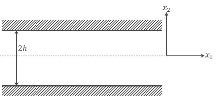
Figure 2.1: Channel flow

The same mathematical formulation can be applied to flow in a different configuration. In the case of planar channel flow as illustrated in figure 2.1, the $x_{1}$ and $x_{3}$ directions remain homogeneous, but the wall normal direction $x_{2}$ is constrained by two walls at $x_{2}=\pm h$. For pressure driven channel flow, we set the applied body force to $\mathbf{f}=\left(\frac{1}{\rho}\overline{\frac{\partial P}{\partial x_{1}}},0,0\right)$. In this case, we also non-dimensionalize all lengths by the channel half-height $h$, which yields the following boundary conditions in the $x_{2}$ direction

$$\mathbf{u}(x_{2}=1)=\mathbf{u}(x_{2}=-1)=0$$ (2.17)

and corresponding periodic boundaries imposed in the $x_{1}$ and $x_{3}$ directions.

2.2.1 Chebyshev basis

As an initial foray into the discussion of channel flow, we will adopt the following Fourier-Chebyshev expansion for the velocity and pressure fields:

$$\mathbf{u}(\mathbf{x},t)=\sum_{\mathbf{k}}\hat{\mathbf{u}}^{\mathbf{k}}e^{ik_{0}t}T_{k_{2}}(x_{2})e^{ik_{1}x_{1}+ik_{3}x_{3}},$$ (2.18a)

$$p(\mathbf{x},t)=\sum_{\mathbf{k}}\hat{p}^{\mathbf{k}}e^{ik_{0}t}T_{k_{2}}(x_{2})e^{ik_{1}x_{1}+ik_{3}x_{3}}.$$ (2.18b)

$$\mathbf{f}(\mathbf{x},t)=\sum_{\mathbf{k}}\hat{\mathbf{f}}^{\mathbf{k}}e^{ik_{0}t}T_{k_{2}}(x_{2})e^{ik_{1}x_{1}+ik_{3}x_{3}},$$ (2.18c)

where $k_{2}=0,\,1,\,2...\infty$ and $k_{0,}\,k_{1}\,,k_{3}=-\infty,...-1,\,0,\,1,..\infty$. Although (2.18) does not immediately satisfy the boundary conditions (2.17), it does allow us to explore the nonlinear terms without complicating the algebra at this stage – a fuller discussion of the boundary conditions appears in section 2.2.5.

First, however, the Chebyshev polynomials in representation (2.18) require a choice of orthogonalization in the $x_{2}$ direction. Here we adopt the following inner product between two Chebyshev polynomials $T_{n}$ and $T_{m}$:

$$\left\langle T_{n}(x),\,T_{m}(x)\right\rangle=\int_{-1}^{1}T_{n}(x)T_{m}(x)\frac{1}{\sqrt{1-x^{2}}}\textrm{d}x=\begin{cases}0,&n\neq m\\ \pi,&n=m=0\\ \pi/2,&n=m\neq 0\end{cases}$$ (2.19)

For Chebyshev polynomials, the equivalent product-to-sum rule is

$$T_{j}(x)T_{k}(x)=\frac{1}{2}\left(T_{j+k}(x)+T_{\left|k-j\right|}(x)\right).$$ (2.20)

Inserting (2.20) in (2.19) and making use of the scalar combination function $C^{pq,k}$ results in

$$\left\langle T_{p}T_{q},\,T_{k}\right\rangle =\pi C^{pq,k}\left(\frac{1+\delta^{k0}}{2}\right)+\frac{\pi}{2}\left(C^{p(-q),k}+C^{(-p)q,k}\right)$$

$$\equiv\mathfrak{C}^{pq,k}$$

and yields the appropriate combination function $\mathfrak{C}^{pq,k}$ for Chebyshev polynomials. To express the multiplication of two functions $h(\mathbf{x},t)=f(\mathbf{x},t)\cdot g(\mathbf{x},t)$, where each function is defined as

$$f(\mathbf{x},t)=\sum_{\mathbf{p}}\hat{f}^{\mathbf{p}}e^{ip_{0}t}T_{p_{2}}(x_{2})e^{ip_{1}x_{1}+ip_{3}x_{3}},\qquad g(\mathbf{x},t)=\sum_{\mathbf{q}}\hat{g}^{\mathbf{q}}e^{iq_{0}t}T_{q_{2}}(x_{2})e^{iq_{1}x_{1}+iq_{3}x_{3}},$$

$$h(\mathbf{x},t)=\sum_{\mathbf{k}}\hat{h}^{\mathbf{k}}e^{ik_{0}t}T_{k_{2}}(x_{2})e^{ik_{1}x_{1}+ik_{3}x_{3}}$$

the spectral coefficients for $\hat{h}^{\mathbf{k}}$ can be written as

$$\hat{h}^{\mathbf{k}}=\sum_{\mathbf{p}}\sum_{\mathbf{q}}\hat{f}^{\mathbf{p}}C^{p_{0}q_{0},k_{0}}C^{p_{1}q_{1},k_{1}}\mathfrak{C}^{p_{2}q_{2},k_{2}}C^{p_{3}q_{3},k_{3}}\hat{g}^{\mathbf{q}}.$$

If we define a composite Fourier-Chebyshev combination matrix as

$$\mathsf{\bar{C}}^{\mathbf{pq},\mathbf{k}}=C^{p_{0}q_{0},k_{0}}C^{p_{1}q_{1},k_{1}}\mathfrak{C}^{p_{2}q_{2},k_{2}}C^{p_{3}q_{3},k_{3}}$$ (2.21)

then the following analogue to (2.4) can be compactly expressed as

$$\hat{h}^{\mathbf{k}}=\sum_{\mathbf{p}}\sum_{\mathbf{q}}\hat{f}^{\mathbf{p}}\mathsf{\bar{C}}^{\mathbf{pq},\mathbf{k}}g^{\mathbf{q}}.$$

2.2.2 Differentiation matrices

In addition to the multiplication of functions, we also will need to handle the differentiation of Chebyshev polynominals using this notation. For the function $f^{\prime}=df/dy$, we examine the following equalities:

$$\frac{d}{dy}f(y)=f^{\prime}(y)=\sum_{k}\hat{f}^{\prime k}T_{k}(y)=\sum_{k}\hat{f}^{k}\frac{d}{dy}T_{k}(y).$$

From Peyret (2013) the relationship between the coefficients $\hat{f}^{\prime k}$ and $\hat{f}^{k}$ can be expressed as

$$\hat{f}^{k}=\frac{2}{1+\delta^{k0}}\sum_{\begin{array}[]{c}p=k+1\\ (p+k)\,\textrm{odd}\end{array}}p\hat{f}^{p}$$

This allows us to express the coefficients $\hat{f}^{\prime k}$ in terms of the original coefficients $\hat{f}^{p}$ using a differentiation matrix $\left(D^{\prime}_{2}\right)^{kp}$:

$$\hat{f^{\prime}}^{k}=\sum_{p}\left(D_{2}^{{}^{\prime}}\right)^{kp}\hat{f}^{p},$$

where the subscript 2 on $D_{2}^{{}^{\prime}}$ indicates the derivative with respect to the $x_{2}$ direction. If we define an equivalent

$$\left(D_{1}^{{}^{\prime}}\right)^{\mathbf{pq}}=-iq_{1}\delta^{\mathbf{pq}},\quad\left(D_{3}^{{}^{\prime}}\right)^{\mathbf{pq}}=-iq_{3}\delta^{\mathbf{pq}},$$

then the resulting gradient matrix is

$$\boldsymbol{\nabla}=\left(\begin{array}[]{ccc}\mathbf{D}^{\prime}_{1}\\ &\mathbf{D}^{\prime}_{2}\\ &&\mathbf{D}^{\prime}_{3}\end{array}\right)=\left(\begin{array}[]{ccc}ik_{1}\delta^{\mathbf{pq}}\\ &\mathbf{D}^{\prime}_{2}\\ &&ik_{3}\delta^{\mathbf{pq}}\end{array}\right)$$

A similar process can be used for the second derivaties $f^{\prime\prime}=d^{2}f/dy^{2}$, where

$$\frac{d^{2}}{dy^{2}}f(y)=f^{\prime\prime}(y)=\sum_{k}\hat{f}^{\prime\prime k}T_{k}(y)=\sum_{k}\hat{f}^{k}\frac{d^{2}}{dy^{2}}T_{k}(y)$$

The relationship between the coefficients $\hat{f}^{{}^{\prime\prime}k}$ and $\hat{f}^{k}$ can be related using the following formula:

$$\hat{f}^{\prime\prime k}=\frac{1}{1+\delta^{k0}}\sum_{p=k+2}^{\infty}p(p^{2}-k^{2})\left[\frac{1+(-1)^{p+k}}{2}\right]\hat{f}^{p}$$

(see Peyret, 2013). This relationship can also be expressed using a second order differentiation matrix $\mathbf{D}_{2}^{{}^{\prime\prime}}$ via

$$\hat{f}^{\prime\prime k}=\sum_{p}\left(D^{{}^{\prime\prime}}\right)^{kp}\hat{f}^{p}.$$

The individual entries in $\mathbf{D}_{2}^{{}^{\prime\prime}}$ can be explicitly written using the following identity for the upper triangular matrix

$$\mathcal{\mathbf{U}}=\frac{\mathbf{I}}{\mathbf{I}-\boldsymbol{\mathcal{P}}}=\left(\begin{array}[]{cccc}1&1&1\\ &1&1\\ &&1&\cdots\\ &&\vdots&\ddots\end{array}\right)$$

where $\boldsymbol{\mathcal{P}}$ is the promotion operator defined in Cheung & Zaki (2014), leading to

$$\left(\mathbf{D}_{2}^{{}^{\prime\prime}}\right)^{kp}=\frac{p(p^{2}-k^{2})}{1+\delta^{k0}}\left[\frac{1+\left(-1\right)^{p+k}}{2}\right]\frac{\left(\boldsymbol{\mathcal{P}}\right)^{2}}{\mathbf{I}-\boldsymbol{\mathcal{P}}}$$ for derivatives in the $x_{2}$ direction. The second order derivatives in the other directions can be written as

$$\left(D_{1}^{{}^{\prime\prime}}\right)^{\mathbf{pq}}=-q_{1}^{2}\delta^{\mathbf{pq}},\quad\left(D_{3}^{{}^{\prime\prime}}\right)^{\mathbf{pq}}=-q_{3}^{2}\delta^{\mathbf{pq}}.$$

From these definitions we can also define a Laplacian operator acting on the variable $\hat{f}^{\mathbf{q}}$:

$$\nabla^{2}\hat{f}^{\mathbf{q}}=\boldsymbol{\Delta}^{\mathbf{pq}}\hat{f}^{\mathbf{q}}=\left(\left(D_{1}^{{}^{\prime\prime}}\right)^{\mathbf{pq}}+\left(D_{2}^{{}^{\prime\prime}}\right)^{\mathbf{pq}}+\left(D_{3}^{{}^{\prime\prime}}\right)^{\mathbf{pq}}\right)\hat{f}^{\mathbf{q}},$$ or

$$\boldsymbol{\Delta^{pq}}=\left(\mathbf{D}_{2}^{{}^{\prime\prime}}\right)^{\mathbf{pq}}-\left(q_{1}^{2}+q_{3}^{2}\right)\delta^{\mathbf{pq}}.$$

2.2.3 The Pressure Poisson Equation

With the Chebyshev basis and differentiation matrices defined in sections 2.2.1 and 2.2.2, the pressure Poisson equation

$$\nabla^{2}p=-\rho\boldsymbol{\nabla\cdot}\left(\mathbf{u}\cdot\boldsymbol{\nabla}\mathbf{u}\right)$$ (2.22)

can then be solved for pressure. Assuming the flow is compressible, the source term on the right hand side is proportional to

$$S=\nabla\cdot\mathbf{u}\nabla\mathbf{u}=\sum_{i,j}\frac{\partial u_{i}}{\partial x_{j}}\frac{\partial u_{j}}{\partial x_{i}}.$$

At each wavenumber $\mathbf{k},$ the source term $S$ can be expressed as

$$S^{\mathbf{k}}=\left(\begin{array}[]{c}\hat{u}_{1}^{\mathbf{p}}\\ \hat{u}_{2}^{\mathbf{p}}\\ \hat{u}_{3}^{\mathbf{p}}\end{array}\right)\left(\begin{array}[]{ccc}\left(-p_{1}\mathsf{\bar{C}}^{,\mathbf{k}}q_{1}\right)&\left(\mathbf{D_{2}^{{}^{\prime}}}\right)^{T}\mathsf{\bar{C}}^{,\mathbf{k}}\left(iq_{1}\right)&\left(-p_{3}\mathsf{\bar{C}}^{,\mathbf{k}}q_{1}\right)\\ \left(ip_{1}\right)\mathsf{\bar{C}}^{,\mathbf{k}}\mathbf{D_{2}^{{}^{\prime}}}&\left(\mathbf{D_{2}^{{}^{\prime}}}\right)^{T}\mathsf{\bar{C}}^{,\mathbf{k}}\mathbf{D_{2}^{{}^{\prime}}}&\left(ip_{3}\right)\mathsf{\bar{C}}^{,\mathbf{k}}\mathbf{D_{2}^{{}^{\prime}}}\\ \left(-p_{1}\mathsf{\bar{C}}^{,\mathbf{k}}q_{3}\right)&\mathbf{\left(\mathbf{D_{2}^{{}^{\prime}}}\right)^{T}}\mathsf{\bar{C}}^{,\mathbf{k}}\left(iq_{3}\right)&\left(-p_{3}\mathsf{\bar{C}}^{,\mathbf{k}}q_{3}\right)\end{array}\right)\left(\begin{array}[]{c}\hat{u}_{1}^{\mathbf{q}}\\ \hat{u}_{2}^{\mathbf{q}}\\ \hat{u}_{3}^{\mathbf{q}}\end{array}\right)$$ (2.23)

using the combination matrix $\overline{\mathsf{C}}^{,\mathbf{k}}$ and differentiation matrices $\mathbf{D}_{2}^{{}^{\prime}}$ defined above. Here we relabel the interior matrix as $B^{\mathbf{pq},\mathbf{k}}$, which allows (2.23) to be compactly written as

$$S^{\mathbf{k}}=\sum_{\mathbf{p},\mathbf{q}}\hat{\mathbf{u}}^{\mathbf{p}}B^{\mathbf{pq},\mathbf{k}}\hat{\mathbf{u}}^{\mathbf{q}}.$$ (2.24)

Inserting (2.24) into (2.22) and inverting to solve for pressure gives

$$\hat{p}^{\mathbf{k}}=-\rho\sum_{\mathbf{l}}\left(\Delta^{-1}\right)^{\mathbf{kl}}\sum_{\mathbf{p},\mathbf{q}}\hat{\mathbf{u}}^{\mathbf{p}}B^{\mathbf{pq},\mathbf{l}}\hat{\mathbf{u}}^{\mathbf{q}}=-\rho\sum_{\mathbf{p},\mathbf{q}}\sum_{\mathbf{l}}\hat{\mathbf{u}}^{\mathbf{p}}\left(\Delta^{-1}\right)^{\mathbf{kl}}B^{\mathbf{pq},\mathbf{l}}\hat{\mathbf{u}}^{\mathbf{q}}.$$ (2.25)

2.2.4 The Navier-Stokes equations

Once the pressure has been found in (2.25), it can be inserted in the Navier-Stokes. From the gradient of pressure

$$\nabla p=\left(\begin{array}[]{ccc}iq_{1}\delta^{\mathbf{pq}}&0&0\\ 0&\left(\mathbf{D}_{2}^{{}^{\prime}}\right)^{\mathbf{pq}}&0\\ 0&0&iq_{3}\delta^{\mathbf{pq}}\end{array}\right)\left(\begin{array}[]{c}\hat{p}^{\mathbf{q}}\\ \hat{p}^{\mathbf{q}}\\ \hat{p}^{\mathbf{q}}\end{array}\right),$$

each direction $m$ and wavenumber $\mathbf{k}$ component can be written as

$$\left(-\frac{1}{\rho}\nabla p\right)_{m}^{\mathbf{k}} = \sum_{\mathbf{r}}D_{m}^{\mathbf{\mathbf{kr}}}\sum_{\mathbf{p},\mathbf{q}}\sum_{\mathbf{s}}\hat{\mathbf{u}}^{\mathbf{p}}\left(\Delta^{-1}\right)^{\mathbf{rs}}B^{\mathbf{pq},\mathbf{s}}\hat{\mathbf{u}}^{\mathbf{q}}$$

$$= \sum_{\mathbf{r},\mathbf{s}}\sum_{\mathbf{p},\mathbf{q}}\hat{\mathbf{u}}^{\mathbf{p}}\left\{D_{m}^{\mathbf{kr}}\left(\Delta^{-1}\right)^{\mathbf{rs}}B^{\mathbf{pq},\mathbf{s}}\right\}\hat{\mathbf{u}}^{\mathbf{q}}.$$

The corresponding definition of $\boldsymbol{\Gamma}_{ij,m}^{\mathbf{pq},\mathbf{k}}$ for channel flow is

$$\boldsymbol{\Gamma}_{ij,m}^{\mathbf{pq},\mathbf{k}}=\left(\begin{array}[]{ccc}0&0&q_{1}\mathsf{\bar{C}}^{,\mathbf{k}}\\ 0&0&-i\mathsf{\bar{C}}^{,\mathbf{k}}\mathbf{D}^{\prime}_{2}\\ 0&0&q_{3}\mathsf{\bar{C}}^{,\mathbf{k}}\end{array}\right)\left(\begin{array}[]{ccc}0&\mathbf{I}&0\\ 0&0&\mathbf{I}\\ \mathbf{I}&0&0\end{array}\right)^{(m)}$$

Combining all of the nonlinear terms in $N_{ij,m}^{\mathbf{pq},\mathbf{k}}$, we have

$$N_{ij,m}^{\mathbf{pq},\mathbf{k}}=i\boldsymbol{\Gamma}_{ij,m}^{pq,k}-\sum_{\mathbf{r},\mathbf{s}}\left[D_{m}^{\mathbf{kr}}\left(\Delta^{-1}\right)^{\mathbf{rs}}B^{\mathbf{pq},\mathbf{s}}\right]$$

Using $\boldsymbol{\Delta}^{\mathbf{pk}}$ defined above, the linear terms of the Navier-Stokes can be grouped into

$$L_{im}^{\mathbf{p}\mathbf{k}}=\left(ip_{0}\delta^{\mathbf{pk}}+\nu\boldsymbol{\Delta}^{\mathbf{pk}}\right)\delta_{im}.$$

Putting everything together, the Navier-Stokes equations can be written as

$$Z_{m}^{\mathbf{k}}(\hat{\mathbf{u}})=\sum_{i}\sum_{\mathbf{p}}L_{im}^{\mathbf{p}\mathbf{k}}\hat{u}_{i}^{\mathbf{p}}+\sum_{ij}\sum_{\mathbf{p,q}}\hat{u}_{i}^{\mathbf{p}}N_{ij,m}^{\mathbf{pq},\mathbf{k}}\hat{u}_{j}^{\mathbf{q}}+\hat{f}_{m}^{\mathbf{k}}=0.$$ (2.26)

and it again becomes possible to express the Navier-Stokes equations as

$$\sum_{i,j}\sum_{\mathbf{p},\mathbf{q}}\left(\hat{u}_{i}^{\mathbf{p}}+\hat{\zeta}_{i}^{\mathbf{p}}\right)^{T}\left(\textsf{N}_{ij,m}^{\mathbf{pq},\mathbf{k}}\right)\left(\hat{u}_{j}^{\mathbf{q}}+\hat{\zeta}_{j}^{\mathbf{q}}\right)=\hat{R}_{m}^{\mathbf{k}}.$$

2.2.5 Satisfying boundary conditions

As mentioned previously, equations (2.26) are not necessarily guaranteeed to satisfy the boundary conditions (2.17) if the Chebyshev polynomials are used directly in representation (2.18). However, this problem can be solved by taking a special combnation of Chebyshev functions

$$\phi_{m}(x_{2})=T_{m}(x_{2})-T_{m^{\prime}}(x_{2})$$ (2.27)

where

$$m^{\prime}=\begin{cases}0,&m\textrm{ even}\\ 1,&m\textrm{ odd}\end{cases}$$

and the index $m$ now varies from $m=2,3,4,5...$ This ensures that

$$\phi_{m}(\pm 1)=0$$

and the no-slip boundary conditions will be automatically satisfied for any solution of the polynomial system (2.26). Using these functions in the flow field variables gives:

$$\mathbf{u}(\mathbf{x},t)=\sum_{\mathbf{k}}\hat{\mathbf{u}}^{\mathbf{k}}e^{ik_{0}t}\phi_{k_{2}}(x_{2})e^{ik_{1}x_{1}+ik_{3}x_{3}},$$ (2.28a)

$$p(\mathbf{x},t)=\sum_{\mathbf{k}}\hat{p}^{\mathbf{k}}e^{ik_{0}t}\phi_{k_{2}}(x_{2})e^{ik_{1}x_{1}+ik_{3}x_{3}}.$$ (2.28b)

$$\mathbf{f}(\mathbf{x},t)=\sum_{\mathbf{k}}\hat{\mathbf{f}}^{\mathbf{k}}e^{ik_{0}t}\phi_{k_{2}}(x_{2})e^{ik_{1}x_{1}+ik_{3}x_{3}}.$$ (2.28c)

It can be shown that the differentiation matrices $\mathbf{D}^{\prime}_{2}$ and $\mathbf{D}^{\prime\prime}_{2}$ do not require modification with the new basis. However, the combination matrix takes a more complicated form. If we project the nonlinear product $\phi_{m}\phi_{n}$ back onto the basis $\phi_{k}$ using the same inner product, we have

$$\left\langle\phi_{m}\phi_{n},\phi_{k}\right\rangle = \left\langle\left(T_{m}-T_{m^{\prime}}\right)\left(T_{n}-T_{n^{\prime}}\right),\left(T_{k}-T_{k^{\prime}}\right)\right\rangle$$

$$= \left\langle T_{m}T_{n}-T_{m^{\prime}}T_{n}-T_{m}T_{n^{\prime}}+T_{m^{\prime}}T_{n^{\prime}},\left(T_{k}-T_{k^{\prime}}\right)\right\rangle$$

$$= \left\langle T_{m}T_{n},T_{k}\right\rangle-\left\langle T_{m^{\prime}}T_{n},T_{k}\right\rangle-\left\langle T_{m}T_{n^{\prime}},T_{k}\right\rangle+\left\langle T_{m^{\prime}}T_{n^{\prime}},T_{k}\right\rangle$$

$$+\left\langle T_{m}T_{n},T_{k^{\prime}}\right\rangle-\left\langle T_{m^{\prime}}T_{n},T_{k^{\prime}}\right\rangle-\left\langle T_{m}T_{n^{\prime}},T_{k^{\prime}}\right\rangle+\left\langle T_{m^{\prime}}T_{n^{\prime}},T_{k^{\prime}}\right\rangle$$

$$= \mathfrak{C}^{mn,k}-\mathfrak{C}^{m^{\prime}n,k}-\mathfrak{C}^{mn^{\prime},k}+\mathfrak{C}^{m^{\prime}n^{\prime},k}+\mathfrak{C}^{mn,k^{\prime}}-\mathfrak{C}^{m^{\prime}n,k^{\prime}}-\mathfrak{C}^{mn^{\prime},k^{\prime}}+\mathfrak{C}^{m^{\prime}n^{\prime},k^{\prime}}$$

$$= \breve{C}^{mn,k}$$

The composite combination function is then

$$\mathsf{\bar{C}}^{\mathbf{pq},\mathbf{k}}=C^{p_{0}q_{0},k_{0}}C^{p_{1}q_{1},k_{1}}\breve{C}^{p_{2}q_{2},k_{2}}C^{p_{3}q_{3},k_{3}}.$$ (2.29)

Using the modified composite combination function (2.29) in the governing equations (2.26) then allows the flow field to satisfy the no-slip boundary conditions (2.17).

3 Solvability

The results of section (2) showed how the nonlinear Navier-Stokes equations could be converted into a series of quadratic polynomials, whose solution lies at the intersection of the entire system. Fortunately, a significant amount of literature in commutative algebra is devoted towards finding the common root of for systems of polynomials (Emiris et al., 2010; Cox et al., 1992), and can be applied in this case. In the next two sections, we explore how the theory of polynomial resultants and Groebner Basis can be used to determine the solvability and find all possible spectral solutions to the Navier-Stokes equations, if they exist.

The solvability of a system of polynomial equations such as (2.12) or (2.26) can be determined through the use of polynomial resultants. Due to its extensive body of literature, a complete summary the theory of resultants is omitted here for conciseness, although additional details can be found in Cox et al. (2006). For the purposes of this work, we define the resultant of a system of polynomials as an algebraic function of their coefficients which is zero if and only if the polynomials contain a common root. For example, given two polynomials $f(x)$ and $g(x)$ defined as

$$f(x)=a_{n}x^{n}+...+a_{1}x^{1}+a_{0},$$

$$g(x)=b_{m}x^{m}+...+b_{1}x^{1}+b_{0}$$

the resultant $R(f,g)$ of $f$ and $g$ is defined as

$$R(f,g)=a_{n}^{m}b_{m}^{n}\left(\prod_{i=1}^{n}\prod_{j=1}^{m}\left(\alpha_{i}-\beta_{j}\right)\right),$$

where $\alpha_{i}$ and $\beta_{i}$ are the roots of $f$ and $g$, respectively. In the case where both $f$ and $g$ are second order polynomials,

$$f(x)=a_{2}x^{2}+a_{1}x^{1}+a_{0}$$

$$g(x)=b_{2}x^{2}+b_{1}x^{1}+b_{0}$$

the resultant can be defined in terms of the determinant of the Sylvester matrix (Sylvester, 1853) and the coefficients $a_{n}$ and $b_{n}$, or

$$R(f,g)=\left|\begin{array}[]{cccc}a_{2}&a_{1}&a_{0}&0\\ 0&a_{2}&a_{1}&a_{0}\\ b_{2}&b_{1}&b_{0}&0\\ 0&b_{2}&b_{1}&b_{0}\end{array}\right|.$$

Therefore, if $f$ and $g$ contain a common root, then

$$R(f,g)=(a_{2}b_{0}-b_{2}a_{0})^{2}-(a_{2}b_{1}-b_{2}a_{1})(a_{1}b_{0}-b_{1}a_{0})=0$$ (3.1)

In the case where $f$ and $g$ are functions of multiple independent variables, the Sylvester resultant is still valid. For example, if both $f=f(x,y,z)$ and $g=g(x,y,z)$ and are quadratic in $z$, we can express them as

$$f(x,y,z)=a_{2}(x,y)z^{2}+a_{1}(x,y)z^{1}+a_{0}(x,y)$$

$$g(x,y,z)=b_{2}(x,y)z^{2}+b_{1}(x,y)z^{1}+b_{0}(x,y)$$

where the coefficients $a_{i}$ and $b_{i}$ are now dependent on $x$ and $y$. The Sylvester resultant can then be computed with respect to $z$ such that

$$R_{z}(f,g)=\left|\begin{array}[]{cccc}a_{2}(x,y)&a_{1}(x,y)&a_{0}(x,y)&0\\ 0&a_{2}(x,y)&a_{1}(x,y)&a_{0}(x,y)\\ b_{2}(x,y)&b_{1}(x,y)&b_{0}(x,y)&0\\ 0&b_{2}(x,y)&b_{1}(x,y)&b_{0}(x,y)\end{array}\right|=0$$

For a system of equations containing more than two polynomials, the resultant of any two arbitrarily chosen polynomials must also be zero for there to be a common root for the entire system. This provides a relatively simple test to determine the solvability of a system of polynomial equations such as (2.12) or (2.26). However, before applying the Sylvester resultant to the current problem, we can make use of a variable substitution to transform the equations into a more suitable form. If we insert

$$\hat{v}_{i}^{\mathbf{k}}=\hat{u}_{i}^{\mathbf{k}}/w$$

into equation (2.12), the result can be written as

$$\mathsf{Z}_{m}^{\mathbf{k}}(\hat{\mathbf{v}}^{\mathbf{k}},w)=2\left(\sum_{i}\sum_{\mathbf{p}}L_{im}^{\mathbf{p}\mathbf{k}}\hat{v}_{i}^{\mathbf{p}}w\right)+\left(\sum_{ij}\sum_{\mathbf{p,q}}\hat{v}_{i}^{\mathbf{p}}\mathcal{\mathsf{N}}_{ij,m}^{\mathbf{pq},\mathbf{k}}\hat{v}_{j}^{\mathbf{q}}\right)+2\hat{f}_{m}^{\mathbf{k}}w^{2}=0.$$ (3.2)

Here the role of $w$ is to serve as a homogenizing variable, and removes some of the arbitrariness in selecting the variable to compute the resultant. Note that each term in (3.2) now has the same degree in either $\hat{v}_{i}^{\mathbf{k}}$ or $w$, making the polynomial $\mathsf{Z}_{m}^{\mathbf{k}}$ homogeneous (not to be confused with the homogeneous nature of the flow in the $x_{1}$ and $x_{3}$ directions). We can then compute the resultant of any two polynomials $\mathsf{Z}_{m}^{\mathbf{k}}$ and $\mathsf{Z}_{m^{\prime}}^{\mathbf{k^{\prime}}}$ with respect to $w$

$$R_{w}(\mathsf{Z}_{m}^{\mathbf{k}},\,\mathsf{Z}_{m^{\prime}}^{\mathbf{k}^{\prime}})=\left|\begin{array}[]{cccc}2\hat{f}_{m}^{\mathbf{k}}&2\sum L_{im}^{\mathbf{p}\mathbf{k}}\hat{v}_{i}^{\mathbf{p}}w&\sum_{ij}\sum_{\mathbf{p,q}}\hat{v}_{i}^{\mathbf{p}}\mathcal{\mathsf{N}}_{ij,m}^{\mathbf{pq},\mathbf{k}}\hat{v}_{j}^{\mathbf{q}}&0\\ 0&2\hat{f}_{m}^{\mathbf{k}}&2\sum L_{im}^{\mathbf{p}\mathbf{k}}\hat{v}_{i}^{\mathbf{p}}w&\sum_{ij}\sum_{\mathbf{p,q}}\hat{v}_{i}^{\mathbf{p}}\mathcal{\mathsf{N}}_{ij,m}^{\mathbf{pq},\mathbf{k}}\hat{v}_{j}^{\mathbf{q}}\\ 2\hat{f}_{m^{\prime}}^{\mathbf{k}^{\prime}}&2\sum L_{im^{\prime}}^{\mathbf{p}\mathbf{k^{\prime}}}\hat{v}_{i}^{\mathbf{p}}w&\sum_{ij}\sum_{\mathbf{p,q}}\hat{v}_{i}^{\mathbf{p}}\mathcal{\mathsf{N}}_{ij,m^{\prime}}^{\mathbf{pq},\mathbf{k}^{\prime}}\hat{v}_{j}^{\mathbf{q}}&0\\ 0&2\hat{f}_{m^{\prime}}^{\mathbf{k}^{\prime}}&2\sum L_{im^{\prime}}^{\mathbf{p}\mathbf{k^{\prime}}}\hat{v}_{i}^{\mathbf{p}}w&\sum_{ij}\sum_{\mathbf{p,q}}\hat{v}_{i}^{\mathbf{p}}\mathcal{\mathsf{N}}_{ij,m^{\prime}}^{\mathbf{pq},\mathbf{k}^{\prime}}\hat{v}_{j}^{\mathbf{q}}\end{array}\right|$$

After some significant algebraic manipulation, the Sylvester resultant can be written as

$$R_{w}(\mathsf{Z}_{m}^{\mathbf{k}},\,\mathsf{Z}_{m^{\prime}}^{\mathbf{k}^{\prime}}) =\sum_{\mathbf{p},\mathbf{q}}\sum_{\mathbf{r},\mathbf{s}}\sum_{i,j}\sum_{l,n}\hat{v}_{i}^{\mathbf{p}}\hat{v}_{j}^{\mathbf{q}}\hat{v}_{l}^{\mathbf{r}}\hat{v}_{s}^{\mathbf{n}} \times\left\{4N_{ij,m}^{\mathbf{pq},\mathbf{k}}N_{ln,m}^{\mathbf{rs},\mathbf{k}}\left(\hat{F}_{m^{\prime}}^{k^{\prime}}\right)^{2}+4N_{ij,m^{\prime}}^{\mathbf{pq},\mathbf{k}^{\prime}}N_{ln,m^{\prime}}^{\mathbf{rs},\mathbf{k}^{\prime}}\left(\hat{F}_{m}^{k}\right)^{2}\right.$$ (3.3)

$$-4N_{ij,m^{\prime}}^{\mathbf{pq},\mathbf{k}^{\prime}}N_{ln,m}^{\mathbf{rs},\mathbf{k}}\hat{F}_{m}^{k}\hat{F}_{m^{\prime}}^{k^{\prime}}-4N_{ij,m}^{\mathbf{pq},\mathbf{k}}N_{ln,m^{\prime}}^{\mathbf{rs},\mathbf{k}^{\prime}}\hat{F}_{m^{\prime}}^{k^{\prime}}\hat{F}_{m}^{k}$$

$$-8L_{im}^{\mathbf{pk}^{\prime}}\hat{F}_{m}^{\mathbf{k}}L_{lm}^{\mathbf{rk}}N_{ij,m^{\prime}}^{\mathbf{pq},\mathbf{k}^{\prime}}-8L_{im}^{\mathbf{pk}}\hat{F}_{m^{\prime}}^{\mathbf{k}^{\prime}}L_{lm^{\prime}}^{\mathbf{rk}^{\prime}}N_{ij,m}^{\mathbf{pq},\mathbf{k}}$$

$$\left.+8L_{im^{\prime}}^{\mathbf{pk}^{\prime}}\hat{F}_{m}^{\mathbf{k}}L_{lm}^{\mathbf{rk}^{\prime}}N_{ij,m}^{\mathbf{pq},\mathbf{k}}-8L_{lm}^{\mathbf{rk}}\hat{F}_{m^{\prime}}^{\mathbf{k}^{\prime}}L_{im}^{\mathbf{pk}}N_{ij,m^{\prime}}^{\mathbf{pq},\mathbf{k}^{\prime}}\right\}=0$$

For a common root to exist for the system (3.2), equation (3.3) must be satisified for any choice of wavenumbers and directions $(\mathbf{k},m)$ and $(\mathbf{k}^{\prime},m^{\prime})$. Note that such a test merely provides a necessary condition for a solution to exist, and not a sufficient condition. To determine the actual solution(s) of the original system, we must apply some additional concepts from commutative algebra.

4 Groebner Basis and a model problem

The results of the previous section provided a set of conditions for which solutions to (3.2) exist. However, they did not provide a means to determine the actual solution(s), if any exist. To illustrate how this might be done, we introduce the idea of a Groebner basis and demonstrate its application on a model nonlinear problem.

Before proceeding, we should note that multiple methods exist for solving systems such as (3.2), and each method possesses its own particular set of advantages and disadvantages. The method of Groebner basis described below is merely one which is relatively quick to implement for simple problems and provides a solid theoretical foundation for further exploration. In the section below, we also consider solutions for a finite set of polynomials.

Defined mathematically, given a set of polynomials $I=\{f_{1}(x_{1},x_{2},...),\,f_{2}(x_{1},x_{2},...),\,...,f_{n}(x_{1},x_{2},...)\}$ and a particular monomial ordering for $(x_{1},x_{2},...)$, the polynomials $G=\{g_{1},\,g_{2},..,g_{n}\}$ is a Groebner basis of polynomials if and only if the leading term of any element in $I$ is divisible by one of the leading terms in $G$. From this definition a significant number of results can be derived, many of which are discussed in (Cox et al., 1992, 2006) and other literature. For the current work, though, we focus on two properties of the Groebner basis which are relevant to our application. First, it can be shown that for the system of equations

$$f_{1}(x_{1},x_{2},...) = 0$$ (4.1a)

$$f_{2}(x_{1},x_{2},...) = 0$$

$$\vdots$$

$$f_{n}(x_{1},x_{2},...) = 0$$ (4.1c)

to have a common solution, the Groebner basis cannot contain the polynomial $g_{i}=1$. This provides a convenient test for the solvability of a system of polynomial equations.

The second remarkable property is that the set of polynomials in a Gröbner basis (set equal to zero) has the same collection of roots as the original polynomials. That is, the solution to

$$g_{1}(x_{1},x_{2},...) = 0$$ (4.2a)

$$g_{2}(x_{1},x_{2},...) = 0$$

$$\vdots$$

$$g_{n}(x_{1},x_{2},...) = 0$$ (4.2c)

is the same solution to (4.1). Furthermore, the system (4.2) can be solved in a much easier fashion compared to (4.1). Due to the eliminiation theorem (Cox et al., 1992), we are guaranteed that one of the equations (4.2) will contain one of the variables $x_{i}$ in isolation, and can be solved for algebraically. After $x_{i}$ is found, it can be used to eliminate another variable $x_{i^{\prime}}$, and so on until the entire system is solution. In this manner, using the Groebner basis is similar to solving a linear system of equations by LU decomposition and backsubstiution. In fact, finding a Groebner basis for a linear system of multiple variaible is equivalent to Gaussian elimination, and for univariate polynomials, it is equivalent to the Euclidian algorithm. An added feature to solving system of polynomial equations via Groebner bases is that all solutions, if they exist, can be found.

The first algorithm for generating a Groebner basis from a set of polynomials was given by Buchberger (Buchberger, 1976) and briefly described in Appendix A. Since that seminal work, alternative algorithms have been developed to generate Groebner basis which are more computationally efficient, but for the purposes of the current analysis and the model problem discussed below, Buchberger’s simple algorithm more than suffices.

4.0.1 Model problem

To illustrate how the Groebner basis can be used to solve nonlinear differential equations, we consisder a one-dimensional ordinary differential equation

$$\frac{d^{2}u}{dx^{2}}+u^{2}-f=0$$ (4.3)

for $u(x)$ and a forcing function $f(x)$ over the domain $0\leq x\leq 2\pi$, with the periodic boundary conditions

$$u(0)=u(2\pi),\qquad f(0)=f(2\pi).$$

While not as complex as the Navier-Stokes (2.1), equation (4.3) contains the necessary nonlinear features to demonstrate the procedure. Similar to 2.2, we use the Fourier representation

$$u(x)=\sum_{k}\hat{u}^{k}e^{ikx},\qquad f(x)=\sum_{k}\hat{f}^{k}e^{ikx}$$ (4.4)

Inserting (4.4) into (4.3) and using the combination matrix gives

$$Z^{k}(\hat{u}^{i})=-k^{2}\hat{u}^{k}+\sum_{p,q}\hat{u}^{p}C^{pq,k}\hat{u}^{q}+\hat{f}^{k}=0,\quad\textrm{for }k=-\infty,...-1,0,1,...\infty$$ (4.5)

An equivalent representation of (4.5) for each polynomial $Z^{k}$ is

$$\hat{Z}^{k}(\hat{u}^{i})=\sum_{p,q}\left(\begin{array}[]{c}\hat{u}^{p}\\ 1\end{array}\right)\cdot\left(\begin{array}[]{cc}2C^{pq,k}&-p^{2}\delta^{pk}\\ -q^{2}\delta^{qk}&2\hat{f}^{k}\end{array}\right)\left(\begin{array}[]{c}\hat{u}^{q}\\ 1\end{array}\right),$$ (4.6)

However, to apply Buchberger’s algorithm, we must choose a finite set of polynmials. Therefore, we truncate all wavenumbers greater than $N$ to result in the following system of polynomial equations:

$$Z^{k}(\hat{u}^{i})=-k^{2}\hat{u}^{k}+\sum_{\left|p\right|,\left|q\right|\leq N}\hat{u}^{p}C^{pq,k}\hat{u}^{q}+\hat{f}^{k}=0,\quad\textrm{for }k=-N,...-1,0,1,...N$$ (4.7)

To apply Buchberger’s algorithm to (4.7), we choose to use a graded reverse lexographic ordering of monomials. Note that the choice of ordering does not affect the resulting Groebner basis, although the efficiency of the algorithm can vary.

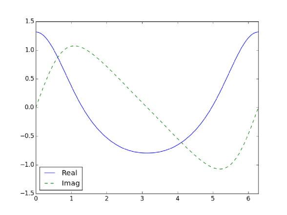
Figure 4.1: The solution to the model problem (4.3) with $f(x)=e^{ix}$ using $N=4$.

In the following example, we choose the forcing function $f(x)=e^{ix}$ and truncate the system of polynomials. For the case where $N=2$, the Groebner basis polynomials are

$$\hat{u}^{-2}=0$$ (4.8a)

$$\hat{u}^{-1}=0$$ (4.8b)

$$9\hat{u}^{0}-8\hat{u}^{2}+2=0$$ (4.8c)

$$9\hat{u}^{1}-16\hat{u}^{2}-5=0$$ (4.8d)

$$16(\hat{u}^{2})^{2}-8\hat{u}^{2}+1=0$$ (4.8e)

Note that equation (4.8e) can be solved directly for $\hat{u}^{2}$ and substituted in the remaining equations to generate the one possible solution to the entire system, yielding

$$\hat{u}^{-2}=\hat{u}^{-1}=\hat{u}^{0}=0,\quad\textrm{and }\hat{u}^{1}=1,\,\hat{u}^{2}=1/4$$ (4.9)

If we retain all Fourier coefficients $\hat{u}^{k}$ for $\left|k\right|\leq 3$, then the Groebner basis polynomials using graded reverse lexographic ordering are

$$\hat{u}^{-3}=0$$ (4.10a)

$$\hat{u}^{-2}=0$$ (4.10b)

$$\hat{u}^{-1}=0$$ (4.10c)

$$121\hat{u}^{0}-324\hat{u}^{3}+18=0$$ (4.10d)

$$121\hat{u}^{1}-648\hat{u}^{3}-85=0$$ (4.10e)

$$242\hat{u}^{2}-729\hat{u}^{3}-20=0$$ (4.10f)

$$324(\hat{u}^{3})^{2}-36\hat{u}^{3}+1=0$$ (4.10g)

which can be further simplified to give the one possible solution:

$$\hat{u}^{-3}=\hat{u}^{-2}=\hat{u}^{-1}=\hat{u}^{0}=0,\quad\textrm{and }\hat{u}^{1}=1,\,\hat{u}^{2}=1/4,\,\hat{u}^{3}=1/18$$ (4.11)

Both solutions given by (4.9) and (4.11) can be verified by direct substitution into the original equation (4.3). Furthermore, from solutions (4.9) or (4.11), one can calculate the remaining coefficients $\hat{u}^{k}$ for $\left|k\right|>N$ through relatively simple algebra. A graph of the solution $u(x)$ is shown in figure 4.1.

A simple visualization of the quadratic polynomials $Z^{k}=0$ is possible if we allow two coefficients $\hat{u}^{k}$ and $\hat{u}^{k^{\prime}}$to vary while fixing all other coefficients at the common root. An example is shown in figure 4.2 where selected polynomials $Z^{k}(\hat{u}^{1},\hat{u}^{2})=0$ and $Z^{k}(\hat{u}^{2},\hat{u}^{3})=0$ are plotted. Depending on the choice of $k$, the resulting curves are either parabolas, hyperbolics, or collapse to straight lines on the particular plane. However, all of the curves intersect at the solution point as expected.

Figure 4.2: Plot of the polynomials (a) $Z^{1}=0$, $Z^{2}=0$, $Z^{3}=0$,$Z^{4}=0$ in the $\hat{u}^{1}$-$\hat{u}^{2}$ plane, and (b) $Z^{2}=0$, $Z^{3}=0$, $Z^{4}=0$ in the $\hat{u}^{2}$-$\hat{u}^{3}$ plane. The solution lies at the intersection of the displayed curves.

5 Discussion

The main results of the previous sections can be summarized as follows: Using the combination matrix $C^{\mathbf{pq},\mathbf{k}}$, the Navier-Stokes equations can be rewritten in terms of intersecting quadratic polynomials (2.13), where the solutions to the system are determined by the number of intersections to the polynomial system. This is shown both for the case of homogeneous isotropic turbulence and planar channel flow using the Chebyshev polynomial basis. Once the polynomial coefficients are known, a solvability condition can be derived, and the solution to these systems can then be solved using standard methods from commutative algebra. For instance, Buchberger’s algorithm can be applied to transform the polynomial system into a Groebner basis, which can then be solved to reveal the common roots. This process is demonstrated for a simple nonlinear differential equation.

Several key points are worth noting regarding this analysis. While we show that the combination can be defined for the Fourier and Chebyshev bases, it can also be extended to other orthogonal polynomials by considering the Clebsch-Gordan or standard linearization problem (Sanchez-Ruiz et al., 1999). Secondly, the method used to determine the Groebner basis in section 4, while useful to illustrate the procedure on simple problems, does not efficiently scale to larger problems. Buchberger’s original algorithm is numerically unstable and diffcult to parallelize to tackle large systems of polynomials. While more efficient methods of finding a Groebner basis are available, it is also possible to use multivariate resultants (similar to those discussed in section 3) to solve the polynomial system (2.13). These methods (Hanzon & Hazewinkel, 2006) convert the system to a standard eigenvalue problem, wihch can then be solved using standard approaches from numerical linear algebra to yield all possible solutions to the original problem. Implementing such an algorithm is more involved than the method described in Appendix A, but if done properly, will yield the same result for the Navier-Stokes.

Appendix A Appendix: Buchberger’s Algorithm

As mentioned in section 4, Buchberger’s algorithm was the first known method for transforming a set of polynomials into a Groebner basis given a particular monomial ordering. This algorithm relies on the creation of an S-polynomial for two polynomials $f$ and $g$, defined as

$$S(f,g)=\textrm{LCM}(\textrm{LPP}(f),\textrm{LPP}(g))\left(\frac{f}{\textrm{LM}(f)}-\frac{g}{\textrm{LM}(g)}\right)$$

where $\textrm{LPP}(f)$ is the leading power product of the polynomial $f$, $\textrm{{LM}}(f)$ is the leading monomial of $f$, and $\textrm{LCM}(f,g)$ is the least common multiple of $f$ and $g$. From this, Buchberger’s method for generating a Groebner basis can be roughly implemented as described in algorithm 1.

Input: $F=(f_{1},...,f_{s})$

Output: a Groebner basis $G=\left\{g_{1},...,g_{t}\right\}$ for $I=\left\langle F\right\rangle$, with $F\subset G$

   LET G := F

   REPEAT

      $G^{\prime}$ := $G$

      FOR each $\left(p,q\right)$ pair $p\neq q$ in $G^{\prime}$ DO

         S := REM{$S(p,q)$}

         IF $S\neq 0$ THEN $G=G\cup\left\{S\right\}$

   UNTIL $G=G^{\prime}$

Algorithm 1 Buchberger’s algorithm, as described in Cox et al. (2006)

References

• Buchberger (1976) Buchberger, B. 1976 A theoretical basis for the reduction of polynomials to canonical forms. ACM SIGSAM Bulletin 10ย (3), 19โ€“29.
• Cheung & Zaki (2014) Cheung, L.ย C. & Zaki, T.ย A. 2014 An exact representation of the nonlinear triad interaction terms in spectral space. Journal of Fluid Mechanics 748, 175โ€“188.
• Cox etย al. (1992) Cox, D., Little, J. & Oโ€™shea, D. 1992 Ideals, varieties, and algorithms, , vol.ย 3. Springer.
• Cox etย al. (2006) Cox, D.ย A., Little, J. & Oโ€™shea, D. 2006 Using algebraic geometry, , vol. 185. Springer Science & Business Media.
• Emiris etย al. (2010) Emiris, I.ย Z., Pan, V.ย Y. & Tsigaridas, E.ย P. 2010 Algorithms and theory of computation handbook. chap. Algebraic and Numerical Algorithms, pp. 17โ€“17. Chapman & Hall/CRC.
• Hanzon & Hazewinkel (2006) Hanzon, B. & Hazewinkel, M. 2006 Proceedings of the colloquiumโ€™constructive algebra and systems theoryโ€™, amsterdam, november 2000. Royal Netherlands Academy of Arts and Sciences.
• Peyret (2013) Peyret, R. 2013 Spectral methods for incompressible viscous flow, , vol. 148. Springer Science & Business Media.
• Sanchez-Ruiz etย al. (1999) Sanchez-Ruiz, J., Artes, P.ย L., Martinez-Finkelshtein, A. & Dehesa, J.ย S. 1999 General linearization formulae for products of continuous hypergeometric-type polynomials. Journal of Physics A: Mathematical and General 32ย (42), 7345.
• Sylvester (1853) Sylvester, J.ย J. 1853 On a theory of the syzygetic relations of two rational integral functions, comprising an application to the theory of sturmโ€™s functions, and that of the greatest algebraical common measure. Philosophical transactions of the Royal Society of London 143, 407โ€“548.