An Algorithmic Framework for Labeling Road Maps

Abstract

Given an unlabeled road map, we consider, from an algorithmic perspective, the cartographic problem to place non-overlapping road labels embedded in their roads. We first decompose the road network into logically coherent road sections, e.g., parts of roads between two junctions. Based on this decomposition, we present and implement a new and versatile framework for placing labels in road maps such that the number of labeled road sections is maximized. In an experimental evaluation with road maps of 11 major cities we show that our proposed labeling algorithm is both fast in practice and that it reaches near-optimal solution quality, where optimal solutions are obtained by mixed-integer linear programming. In comparison to the standard OpenStreetMap renderer Mapnik, our algorithm labels $31\%$ more road sections in average.

1 Introduction

Due to the increasing amount of geographic data and its steady change, automatic approaches become more and more important in the area of cartography. This particularly applies to the time-consuming and demanding task of label placement and much research has been done on its automation. Badly placed labels of feature of interest make maps easily unreadable [5]. Depending on the type of map feature the label placement is done differently. For point features (e.g., cities on small-scale maps) labels are typically placed closely to that feature, while for line features (e.g., roads, rivers) the name is either placed along or inside the feature. The latter approach is also used for area features (e.g., lakes). Independently of the applied technique and feature type, labels should not overlap each other and clearly identify the features [8].

The cartographic label placement problem has also attracted the interest of researchers in computational geometry and it has been thoroughly investigated from both the practical and theoretical perspective [14, Chapter 58.3.1], [16]. While algorithms for labeling point features got a lot of attention, much less work has been done on line features and area features. In this paper we address labeling line features, namely labeling the entire road network of a road map. We take an algorithmic, mathematical perspective on the underlying optimization problem and build up on our recent theoretical results for labeling tree-shaped networks [4]. We apply the quality criteria for label placement in road maps elaborated by Chirié [2] based on interviews with cartographers. They include that (C1) labels are placed inside and parallel to the road shapes, (C2) every road section between two junctions should be clearly identified, and (C3) no two road labels may intersect. Similar criteria have been described in a classical paper by Imhof [5].

Variations of embedded labels have been considered in road maps before. Chirié [2] and Strijk et al. [12, Ch. 9] presented simple, local heuristics that place non-overlapping labels based on a discrete set of candidate positions – in contrast we consider the problem globally applying a continuous sliding model. Seibert and Unger [11] utilized the geometric properties of grid-based road networks and proved that it is NP-complete to decide whether at least one label can be placed for each road. For the same grid-based setting Neyer and Wagner [7] evaluated a practically efficient algorithm that is not applicable for general road networks.

Road labeling with embedded labels has also been considered for interactive and dynamic maps. Maass and Döllner [6] provided a heuristic for labeling interactive 3D road maps taking obstacles into account. Vaaraniemi et al. [13] presented a study on a force-based labeling algorithm for dynamic maps considering both point and line features. Schwartges et al. [10] investigated embedded labels in interactive maps allowing panning, zooming and rotation of the map. They evaluated a simple heuristic for maximizing the number of placed labels.

In contrast, non-embedded labels are typically considered for single line features such as rivers. Edmondson et al. [3] presented an algorithm for placing straight labels along single line features. Wolff et al. [15] also considered the case that labels may bend. Recently, Schwartges et al. [9] used billboards (labels with short leaders) for naming roads in interactive 3D maps to avoid label distortion.

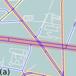
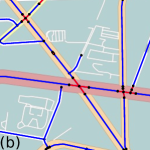
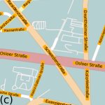
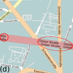
Figure 1: The presented workflow. (a) The road network given by polylines (blue segments). (b) Phase 1: A graph $G$ is created whose embedding is the simplified road network; blue segments: road sections, red segments: junction edges. (c) Phase 2: Creating the labeling using $G$. (d) A labeling produced by the OSM renderer Mapnik. The six labels of road Osloer Straße are enclosed by red ellipses.

(a) Google Maps: Hermann-Vollmerstraße, Karlsruhe (Germany)

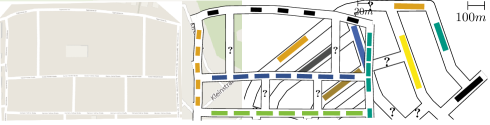
(b) Bing Maps: Kirchbuel, Karlsruhe (Germany)

Figure 2: Two maps of the map services Google Maps and Bing Maps. Left: Screen shot of a road map. Right: The redrawn road map to emphasize the labels. Labels of the same color belong to the same road. 2(a) Labels are placed tightly packed in a row. While some roads have more labels then necessary, other roads are not labeled. 2(b) Road map consists of many unlabeled road sections.

For labeling point features a typical objective is to maximize the number of non-overlapping placed labels, because every placed label enhances the map with further information. While this is mostly true for point features, maximizing the number of labels is not the right objective for label placement of roads since not every label that is placed necessarily contributes more information to the map. For example, consider the placed labels of the road Osloer Straße in Fig. 1(d). We can easily remove some of those labels without losing any information, because the map user can still identify the same road sections; see Fig. 1(c). In online map services, however, one often can find such redundant labels; see Fig. 2 for two examples. Some roads may have unnecessarily many labels, which may in turn cause others to remain completely unlabeled. Hence, the user cannot identify such roads on the map, a real disadvantage if headed for that road. Due to these observations we do not aim to maximize the number of labels, but the number of labeled road sections. For the purpose of this paper, a road section forms a connected piece of the road network that logically belongs together, e.g., a part of a road between two junctions or a part that stands out by its color or width. Our algorithm, however, is independent of the actual definition of road sections; any partition of the road network into disjoint road sections can be handled. We say that a road section is labeled if a label (partly) covers it.

As the underlying model for maximizing labeled road sections we re-use the planar graph model that has been introduced in our theoretical companion paper [4]. In that paper we further proved that labeling a maximum number of road sections is NP-hard, even for planar graphs and if no road consists of multiple branches. However, we presented a polynomial-time algorithm for the case that the road graph is a tree. While the result for trees is mostly of theoretic interest (road networks rarely form trees), we will show in this paper that our tree-based algorithm can in fact be used successfully as the core of an efficient and practical road labeling algorithm that produces near-optimal solutions.

Contribution & Outline.

We introduce a new, versatile algorithmic framework for placing non-overlapping labels in road networks maximizing the number of labeled road sections. We keep the algorithmic components easily exchangeable. In Sect. 2 we discuss and expand the model introduced in [4]. Afterwards, we present a workflow for labeling road networks consisting of two phases; see Fig. 1.

Phase 1 (Sect. 3). We translate the given road network into a semantic representation (an abstract road graph) that identifies pieces of the road network that belong semantically together. To that end, we simplify the road network, e.g., we merge lanes closely running in parallel. By design this simplification maintains the overall geometry of the road network and only merges structures in the data that should not be labeled independently. Phase 1 is not part of the labeling optimization process.

Phase 2 (Sect. 4). Based on the abstract road graph, we create an actual labeling using one of three presented algorithms: a naive base-line algorithm, a heuristic extending our tree-based algorithm [4] and a mixed-integer linear programming (MILP) formulation.

As proof of concept we implemented the core of the framework only taking the most important cartographic criteria into account. However, with some engineering it can be easily enhanced to more complex models, e.g., enforcing minimum distances between labels, abbreviating road names, or using alternative definitions of road sections. In Sect. 5 we present a detailed evaluation of our framework on 11 sample city maps. Due to its availability and popularity in practice, we compare our results against the standard OpenStreetMap (OSM) renderer Mapnik as a representative of local heuristics; it uses a strategy similar to [2, 12]. We show that our tree-based algorithm is fast and yields near-optimal labelings that improve upon Mapnik by $31\%$ on average.

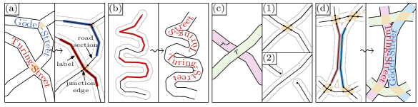
Figure 3: Illustration of model and arising issues. (a) Sketch of a road network and its abstract road graph. (b) Labels are possibly curvy and have sharp bends making the text hardly legible. (c) Issue 2: Two ways to represent bridges and tunnels in the abstract road graph. (d) Issue 4: The text representation of labels may overlap, while the curve representation in the abstract road graph does not.

2 Semantic Representation of Road Networks

At any given scale, road networks are typically drawn as follows. Each road or road lane is represented as a thick, polygonal curve, i.e., a polygonal curve with non-zero width; see the background of Fig. 1(a). If two (or more) such curves intersect, they form junctions. If two or more lanes of the same road closely run in parallel they merge to one even thicker curve such that individual lanes become indistinguishable. We then want to place road labels inside those thick curves. More precisely, a road label can again be represented as a thick curve (the bounding shape of the road name) that is contained in and parallel to the thick curve representing its road; see Fig. 1(c).

For the purpose of this paper it is sufficient to use a simplified representation, which represents the road network and its labels as thin curves instead [4]. More precisely, a road network is modeled as a planar embedded abstract road graph whose edges correspond to the skeleton of the actual thick curves. In this model a label is again a thin curve of certain length that is contained in the skeleton. Following the cartographic quality criteria (C1)–(C3), we want to place labels, i.e., find sub-curves of the skeleton, such that (1) each label starts and ends on road sections, but not on junctions, (2) no two labels overlap, and (3) a maximum number of road sections are labeled. Requiring that labels end on road sections avoids ambiguous placement of labels in junctions where it is otherwise unclear how the road passes through it. Note that this does not forbid labels across junctions. From a labeling of the abstract road graph it is straight-forward to transform each label back into its text representation by placing the individual letters of each label along the thick curves; see Fig. 3(a).

Abstract Road Graph Model.

We have introduced the abstract road graph in [4], but for the convenience of the reader we repeat it here, see also Fig. 1(b) and Fig. 3(a). A road network (in an abstract sense) is a planar geometric graph $G=(V,E)$, where each vertex $v\in V$ has a position in the plane and each edge $\{u,v\}\in E$ is represented by a polyline whose end points are $u$ and $v$. Each edge further has a road name. A maximal connected subgraph of $G$ consisting of edges with the same name forms a road $R$. The length of the name of $R$ is denoted by $\lambda(R)$. Each edge $e\in E$ is either a road section, i.e., the part of a road in between two junctions, or a junction edge, which models road junctions. Formally, a junction is a maximal connected subgraph of $G$ that only consists of junction edges. We require that no two road sections in $G$ are incident to the same vertex and that vertices incident to road sections have at most degree 2. Thus, the road graph $G$ decomposes into road sections, separated by junctions.

We say a point $p$ lies on $G$, if there is an edge $e\in E$ whose polyline contains $p$. Hence, a polyline $\ell$ (in particular a single line segment) lies on $G$ if each point of $\ell$ lies on $G$. Further, $\ell$ covers $e$, if there is a point of $\ell$ that lies on $e$. If each point of $e$ is covered by $\ell$, $e$ is completely covered. The geodesic distance of two points on $G$ is the length of the shortest polyline on $G$ connecting both points.

A label of a road $R$ is a simple open polyline $\ell$ on $G$ that has length $\operatorname{len}(\ell)=\lambda(R)$, ends on road sections of $G$, and whose segments only lie on edges of $R$. The start point of $\ell$ is denoted as the head $h(\ell)$ and the endpoint as the tail $t(\ell)$. Obviously, the edges that are covered by $\ell$ form a path $\mathcal{P}_{\ell}=(e_{1},e_{2},\cdots,e_{k-1},e_{k})$ such that $e_{1}$, and $e_{k}$ are (partly) covered and $e_{2},\dots,e_{k-1}$ are completely covered by $\ell$. If $e_{i}$ is a road section (and not a junction edge), we say that $e_{i}$ is labeled by $\ell$.

We extend the above abstract road graph model and restrict ourselves to well-shaped labels, i.e., labels that are not too curvy or do not contain broken type setting due to sharp bends; see Fig. 3(b). Similar to Schwartges et al. [10], we apply a local criterion to decide whether a label is well-shaped. To that end, we define a label $\ell$ to be well-shaped if for each covered edge $e\in\mathcal{P}_{\ell}$ there is a well-shaped piece of $e$ that completely contains the part of $\ell$ on $e$. Further, we require that for each pair of incident edges of $\mathcal{P}_{\ell}$ the bend angle is at most $\alpha_{\text{max}}$, where $\alpha_{\text{max}}$ is a pre-defined constant. We redefine a labeling $\mathcal{L}$ to be a set of mutually non-overlapping, well-shaped labels. Our theoretic results [4] remain valid for this restriction. In particular only few minor technical adaptions are required for the tree labeling algorithm.

In order to identify well-shaped pieces of a polyline $P$ with edges $e_{1},\dots,e_{k}$, we extend the approach presented by Schwartges et al. [10]. They define the curviness $w(P)$ of $P$ by summing up the bend angles $\alpha_{i}$ of all incident edge pairs $e_{i}$, $e_{i+1}$, i.e., $w(P)=\sum_{i=1}^{k-1}|\alpha_{i}|$ to determine the best label positions for any given label. We want to locally classify road pieces as well-shaped instead and adapt their idea as follows. Let $S$ be a maximal sub-polyline of $P$ with the property that any sub-polyline of $S$ with length at most $l_{\text{max}}$ has curviness at most $\alpha_{\text{max}}$. Each such sub-polyline $S$ forms a well-shaped piece of $P$ and they can all be computed in $O(k)$ time. This local criterion for well-shapedness is based on the curviness of a fixed-width window sliding along the polyline; it is independent of the label length (similarly to what Mapnik does). In our experiments we set $l_{\text{max}}$ to twice the length of the letter W and $\alpha_{\text{max}}=22.5^{\circ}$, analogously to the parameters that Mapnik uses.

A labeling $\mathcal{L}$ for a road network is a set of mutually non-overlapping, well-shaped labels, where two labels $\ell$ and $\ell^{\prime}$ overlap if they intersect in a point that is not their respective head or tail. Following the criteria (C1)–(C3), the problem MaxLabeledRoads is to find a labeling $\mathcal{L}$ that labels a maximum number of road sections, i.e., no other labeling labels more road sections. In [4] we showed that MaxLabeledRoads is NP-hard in general and can be solved in $O(|V|^{3})$ time if $G$ is a tree.

Shortcomings for Real-world Road Networks.

While the abstract road graph model allows theoretical insights, we cannot directly apply it to real-world road networks. Due to the following issues, we need to invest some effort in a preprocessing phase (see Sect. 3) to guarantee that the resulting labels in the text representation do not overlap, look nicely and are embedded in the roads’ shapes.

Issue 1: If lanes run closely in parallel, their drawings in the road network merge to one thick curve and individual lanes become indistinguishable. Hence, in our abstract model, such lanes should be aggregated to a single road section that represents the skeleton of the merged curve, and labels should be contained in it; see Fig 1(c).

Issue 2: Real-world road networks are not planar, but edges may cross, namely at tunnels and bridges; see Fig. 3(c). To avoid overlaps between labels placed on those road sections, we either can model the intersection as a regular junction of two roads or we split one into two shorter road sections that do not cross the other road section. In both cases the road graph becomes planar. For our prototype we use the first variant (also used by Mapnik), because more road sections can be labeled.

Issue 3: In real-world road networks some road sections are possibly so long that the label should be repeated after appropriate distances.

Issue 4: Labels have a certain font size so that when transforming an abstract label curve into its text representation, labels of different roads may overlap due to their road sections being too close; see Fig. 3(d).

3 Phase 1 – Construction of Abstract Road Graphs

The first phase of our framework consists of transforming the input road network data into an abstract road graph while resolving the four issues mentioned in Sect. 2. Typically, road networks are given as a set of polylines that describe the roads and road lanes. Individual polylines do not necessarily form semantic components such as road sections. So as a first step, we break all polylines down into individual line segments (whose union forms the road network). Let $L$ be the set of all these line segments. We further require that each line segment $l\in L$ is annotated with its road name $\operatorname{rn}(l)$, the stroke width $\operatorname{st}(l)$ and the color $\operatorname{co}(l)$ that are used to draw $l$, and finally the font size $\operatorname{fs}(l)$ that shall be used to display the name. We say that two line segments $l,l^{\prime}\in L$ are equally represented if $\operatorname{st}(l)=\operatorname{st}(l^{\prime})$ and $\operatorname{co}(l)=\operatorname{co}(l^{\prime})$. We assume that $\operatorname{fs}(l)<\operatorname{st}(l)$ for any $l$; otherwise we set $\operatorname{st}(l):=\operatorname{fs}(l)$.

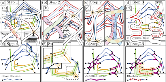
Figure 4: Illustration of the steps applied in Phase 1. Segments of the same color have the same road name. For more details see the description of Phase 1.

The workflow consists of the following five steps; see Fig. 4. (1) Identification.Identify single road components, i.e., sets of line segments that have the same name, are equally represented, and form a connected component. (2) Simplification.Simplify each road component such that lanes running closely in parallel are aggregated. (3) Planarization.Replace bridges and tunnels by artificial junctions. (4) Transformation.Transform the segment representation into an abstract road graph. (5) Resolving Overlaps.Identify mutual overlaps of road sections and block them for label placement.

Below we describe each step in more detail. We define the hull of a line segment $l\in L$ to be the region of points whose Euclidean distance to $l$ is at most $\operatorname{st}(l)$; see Fig. 4(a). The hull of a polyline is then the union of its segments’ hulls. We approximate hulls by simple polygons.

Step 1 – Identification. For each road name $n$, each color $c$ and each font size $f$ we define the intersection graph of the hulls of the line segments $L_{n,c,f}=\{l\in L\mid\operatorname{rn}(l)=n,\ \operatorname{co}(l)=c\text{ and }\operatorname{fs}(l)=f\}$. In this intersection graph each hull is a vertex and two vertices are connected if and only if the corresponding hulls intersect. In each (non-empty) intersection graph we identify all connected components, which we call road components; e.g., in Fig. 4(a) the blue segments form a road component. Thus, based on $L$ we obtain a set $\mathcal{C}$ of road components. By definition, each component $C\in\mathcal{C}$ has a unique name $\operatorname{rn}(C)$, stroke width $\operatorname{st}(C)$, color $\operatorname{co}(C)$ and font size $\operatorname{fs}(C)$.

Step 2 – Simplification. For each road component $C\in\mathcal{C}$ we geometrically form the union of the corresponding hulls. Thus, the result is a simple polygon $P$ (possibly with holes); see Fig. 4(b), top. This polygon describes the contour of the road component as drawn on the map. We discard all polygons whose area is smaller than some threshold as they are too small to be labeled; we use the area of the letter W as threshold. For each remaining polygon $P$ we construct the skeleton of $P$ as a linear representation of the corresponding road component such that labels centered on the skeleton are guaranteed to be contained in $P$. This skeleton is based on the conforming Delaunay triangulation of the interior of $P$ following Bader and Weibel [1]. For triangles that have one or three internal edges, i.e., edges that do not belong to the boundary of $P$, we connect the triangle centroid to the midpoints of the internal edges. For triangles with two internal edges, we simply connect the midpoints of these two edges, see Fig. 4(b), bottom. From those line segments, we form a set of maximal polylines by appending all those line segments that meet at the midpoint of a triangle edge (but not at a triangle centroid). Since these polylines may consist of many vertices and meander locally, we simplify them using the Douglas-Peucker algorithm, but only if the simplified shortcuts keep a distance of at least $\operatorname{fs}(C)/2$ to the boundary of $P$, see Fig. 4(c). Finally, we delete any segment $l$ whose text box $B_{l}$ is not completely contained in $P$. Here the text box $B_{l}$ of $l$ is defined as a rectangle centered at $l$ with two sided parallel to $l$. These parallel sides have the same length as $l$, the two orthogonal sides have length $\operatorname{fs}(C)$, see Fig. 4(b), bottom. Segments with the text box not contained in $P$ may occur at the protrusions of the component where circular arcs are approximated by polylines, see Fig. 4(c), top left. The remaining set of polylines forms the skeleton of $P$.

Thus, for each road component $C$ we obtain a skeleton such that all text boxes of the skeleton edges are contained in $P$. This resolves Issue 1. We annotate each skeleton edge with the name, stroke width, color and font size of $C$.

Step 3 – Planarization. So far polylines of different road components may intersect at other points than their end points, e.g., polylines representing bridges and tunnels may cross other polylines. As motivated in Sect. 2, we subdivide these polylines to resolve intersections; see Fig. 4(d). More precisely, if two line segments $\overline{pq}$ and $\overline{rs}$ of two polylines intersect at a point $t$, we replace them by the four segments $\overline{pt}$, $\overline{tq}$, $\overline{rt}$ and $\overline{ts}$. We do the intersection tests with a certain tolerance to identify $T$-crossings safely. However, this may yield short stubs that protrude junctions slightly; we remove those stubs. Thus, this step resolves Issue 2 and yields a set of annotated polylines only intersecting in vertices.

Step 4 – Transformation. Next we create the abstract road graph from the polylines of the previous step. As a result of Step 3 we know that any two polylines intersect only in vertices. We first take the union of all polylines, identify vertices that are common to two or more polylines and mark these vertices as junction seeds. This induces already a planar graph $G=(V,E)$ with polyline edges whose vertices $V$ are either junction seeds or have degree 1. It remains to partition the edges of $G$ into road sections and junction edges. Initially, we mark all edges as road sections. We distinguish two types of junction seeds in $G$.

If a junction seed $v$ has degree at least $3$, only two of its incident edges $e$ and $e^{\prime}$ belong to the same road $R$ and all other incident edges belong to different roads (and have a different road type than $R$) then we do not create any junction edges at $v$, see Fig. 4(e), small box. Since $R$ is the only road that may use the junction at $v$ and it is visually clear that all other roads end at $v$ we can safely treat $v$ as an internal vertex of a road section of $R$. So we disconnect all incident edges of $v$ except $e$ and $e^{\prime}$ from $v$ and let each of them end at its own slightly displaced copy of $v$. The edges $e$ and $e^{\prime}$ are merged at $v$ and the new edge remains a road section. This resolves the situation as desired.

For all other junction seeds we create junction edges as follows. Let $v$ be a junction seed and let $E_{v}$ be the set of edges incident to $v$. We intersect the hulls of all edges in $E_{v}$ and project their intersection points onto the corresponding edges, see Fig. 4(f). For each edge $e\in E_{v}$ we determine the projection point $p_{e}$ that is farthest away from $v$ (in geodesic distance). If the distance between $p_{e}$ and $v$ exceeds a given threshold $\delta$, we shift $p_{e}$ to the point on $e$ that has distance $\delta$ from $v$. Now we subdivide $e$ at $p_{e}$ and mark the edge $\{v,p_{e}\}$ as a junction edge; the other edge at $p_{e}$ (if non-empty) remains a road section. The threshold $\delta$ ensures that roads running closely in parallel are not completely marked as junction edges. Figure 4(g) shows the resulting abstract road graph.

To resolve Issue 3 we subdivide road sections whose length exceeds a certain threshold (in our experiment 350 pixels) by inserting a very short junction edge.

Step 5 – Resolving Overlaps. By Step 2 the hulls of edges that belong to the same road component do not overlap. However, if two sections of different roads run closely in parallel, their hulls (and hence their labels) may overlap. We identify overlaps of the hulls of non-incident edges in $G$ and block the corresponding parts of the edge whose road is less important for placing labels; ties are broken arbitrarily. More complex approaches using road displacement could be applied, however, we have chosen a simple solution. By design hulls of incident edges may only overlap if both are junction edges; those overlaps are handled by the labeling algorithms; see Sect. 4. This resolves Issue 4.

4 Phase 2 – Label Placement in Road Graphs

In this section we present the four different methods for solving MaxLabeledRoads that we subsequently evaluate in our experiments in Sect. 5. Furthermore, we describe a technique for decomposing road graphs into several smaller, independent components that may speed up computations.

4.1 Labeling Methods

BaseLine. An obvious base-line heuristic to obtain lower bounds is to simply place a well-shaped label on each individual road section that is long enough to admit such a label without extending into any junctions. We use this approach to show that it is beneficial to position labels across junctions.

Mapnik. Mapnik (http://mapnik.org) is a standard open source renderer for OpenStreetMap that includes an road labeling algorithm. The algorithm iteratively labels so-called ways, which are polylines describing line features in OpenStreetMap. Along each way it places labels with a certain spacing and locally ensures that labels do not intersect already placed labels of other ways. It does not use any semantic structure from the road network (e.g., road sections), but relies on how the contributors of OpenStreetMap modeled single ways. We may run the rendering algorithm and extract all placed labels from its output.

Tree. The tree-based heuristic makes use of our recently proposed algorithm that optimally solves MaxLabeledRoads if $G$ is a tree [4]. The basic idea for trees is that a placed label splits the tree into several independent sub-trees, which then are labeled recursively. Using dynamic programming we reuse already computed results so that the algorithm’s complexity becomes polynomial, namely $O(|V|^{5})$ running time and $O(|V|^{2})$ space. Applying some further intricate modifications we improved this to $O(|V|^{3})$ time and $O(|V|)$ space, and $O(|V|^{2})$ time if each road in $G$ is a path. We omit the details and use that algorithm as a black box. If $G$ is a tree, our heuristic optimally labels $G$. Otherwise it computes a spanning tree $T$ on $G$ using Kruskal’s algorithm and computes an optimal labeling for $T$. We construct $T$ such that all road sections of $G$ are contained in $T$. Since a road section is only incident to junction edges, this is always possible. In Sect. 5 we show that large parts of realistic road networks can actually be decomposed into paths and trees without losing optimality.

Milp. In order to provide upper bounds for the evaluation of our labeling algorithms, we implement a mixed-integer linear programming (MILP) model that solves MaxLabeledRoads optimally on arbitrary abstract road graphs. The basic idea is to discretize all possible label positions and to restrict the space of feasible solutions to non-overlapping sets of labels.

We now describe the MILP formulation in detail. To simplify the presentation, we drop the rather technical concept of well-shaped labels, but note that it can be easily incorporated into the MILP. In the following let the edges of $G$ be (arbitrarily) directed.

We first discretize the problem as follows. Two labels $\ell$ and $\ell^{\prime}$ are equivalent if they cover the same edges in the same order, i.e., $\mathcal{P}_{\ell}=\mathcal{P}_{\ell^{\prime}}$, and only their end points differ; see Fig. 5(b). For each such equivalence class we create one label $\ell$; we denote its equivalence class by $\mathcal{K}_{\ell}$. Further, let $L$ denote the set of such created labels. The main idea of the MILP is to select a subset of $L$ and to determine the exact positions of the labels’ end points on their terminals such that they do not overlap and label a maximum number of road sections.

Now, consider a label $\ell\in L$ and the path $\mathcal{P}_{\ell}=(e_{1},e_{2},\cdots,e_{k-1},e_{k})$ that is covered by $\ell$; see Fig. 5(b). In the following we call $e_{1}$ and $e_{k}$ the terminals of $\ell$ and the others internal edges of $\ell$. Assume that the head of the label $\ell$ lies on $e_{1}$ and the tail on $e_{k}$, then $\ell$ can slide along $\mathcal{P}_{\ell}$ changing the covered road sections until the head or tail of $\ell$ hits an end point of $e_{1}$ or $e_{k}$, respectively. At each position, $\ell$ coincides with an equivalent label $\ell^{\prime}$. Obviously, those labels exactly form $\mathcal{K}_{\ell}$. Further, there exist two positions on $e_{1}$ such that the head of $\ell$ has either minimum geodesic distance $a$ or maximum geodesic distance $b$ to the source of $e_{1}$, respectively. We define the interval $H_{\ell}=[a,b]$. Analogously, we define the interval $T_{\ell}$ for the tail of $\ell$ and the edge $e_{k}$.

For each label $\ell\in L$ we introduce the variables $x_{\ell}\in\{0,1\}$, $h_{\ell}\in H_{\ell}$ and $t_{\ell}\in T_{\ell}$, and for each road section $e\in E$ the variable $y_{e}\in\{0,1\}$. We interpret $x_{\ell}=1$ such that $\ell$ is selected for the labeling. The variables $h_{\ell}$ and $t_{\ell}$ are interpreted as the geodesic distances of the head and tail to the source of the head’s and tail’s terminal, respectively; see Fig. 5(c). We interpret $y_{e}=1$ as road section $e$ being labeled and maximize the sum $\sum_{e\in E}y_{e}$ subject to the following constraints.

For each $\ell\in L$ we require

$$\operatorname{cov}(e_{1},\ell)+\operatorname{len}(e_{2})+\ldots+\operatorname{len}(e_{k-1})+\operatorname{cov}(e_{k},\ell)=\operatorname{len}(\ell),$$ (1)

where $\mathcal{P}_{\ell}=(e_{1},\dots,e_{k})$, $\operatorname{len}(\ell)$ denotes the given length of $\ell$ and $\operatorname{cov}(e,\ell)$ is a linear expression describing what length of $e$ is covered by $\ell$. This expression depends on which end point of $e$ is covered, whether the head or tail of $\ell$ lies on $e$, and on the position variables $h_{\ell}$ and $t_{\ell}$, respectively; we omit the technical definition. Further, for each pair $\ell^{\prime},\ell\in L$ we require

$$x_{\ell}+x_{\ell^{\prime}}\leq 1 \ell \ell^{\prime}$$ if an edge of is an internal edge of (2)

$$\begin{split}h_{\ell}-h_{\ell^{\prime}}\leq M(2-x_{\ell}-x_{\ell^{\prime}})&\quad\text{ if the heads of~{}$\ell$ and $\ell^{\prime}$ lie on a common}\\[-3.22916pt] &\quad\text{ terminal~{}$e$ and $\ell$ covers the source of~{}$e$.}\end{split}$$ (3)

For each road section $e\in E$ and all labels $\ell_{1},\dots,\ell_{k}\in L$ labeling $e$ we require

$$y_{e}\leq x_{\ell_{1}}+\cdots+x_{\ell_{k}}$$ (4)

Constraint (1) ensures that each label has the desired length $\operatorname{len}(\ell)$. Constraint (2) ensures that a label does not overlap another label internally, i.e., it (partly) covers an edge that is completely covered by another label. Constraint (3) ensures that labels ending on the same road section do not overlap on that edge, but $\ell$ ends on $e$ before $\ell^{\prime}$ starts; see Fig. 5(c). Similar constraints are introduced for the other combinations on how heads and tails of $\ell$ and $\ell^{\prime}$ can lie on a common edge, and on whether source or target of $e$ is covered. For an appropriate large $M$ the constraint is trivially satisfied if $\ell$ or $\ell^{\prime}$ is not selected for the labeling. Finally, Constraint (4) ensures that road section $e$ is only counted as labeled, if there is at least one selected label covering $e$.

Since $L$ models all possible label positions and the constraints restrict the space of feasible solutions to non-overlapping sets of labels, it is clear that any optimal solution of the above MILP corresponds to an optimal solution of MaxLabeledRoads.

Theorem 1.

Milp solves MaxLabeledRoads optimally.

Finding an optimal solution for a MILP formulation is NP-hard in general and remains NP-hard for the stated formulation, because MaxLabeledRoads is NP-hard. However, it turns out that in practice we can apply specialized solvers to find optimal solutions for reasonably sized instances in acceptable time, see Sect. 5.

4.2 Decomposition of Road Networks.

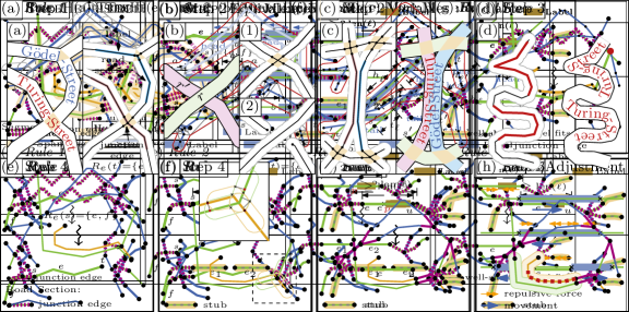
Figure 5: Illustration of the algorithms. Edges of the same color belong to the same road.

We may speed up both our heuristic Tree and the exact approach Milp by decomposing the road graph into smaller, independent components to be labeled separately, i.e., components whose individual optimal solutions compose to a conflict-free optimal solution of the initial road graph. Such a decomposition allows to compute solutions in parallel with either of the above methods and it further decreases the total combinatorial complexity. The decomposition rules guarantee that the labelings of the components can always be merged without creating any label overlaps. We name this technique D&C.

Step 1 – Decomposition. For many road sections, e.g., long sections, of real-world road networks labels can be easily placed preserving the optimal labeling. We iterate through the edges of $G$ and cut or remove some of them if one of the following rules applies. As a result the graph decomposes into independent connected components; see Fig. 5(d)–(g). Let $e$ be the currently considered edge and let $R$ be the road of $e$.

Rule 1. If $e$ is a junction edge and it cannot be completely covered by a well-shaped label, i.e., $e$ is not well-shaped, then remove $e$.

Rule 2. If $e$ is a road section that ends at a junction that is not connected to any other road section of $R$, then detach $e$ from that junction.

Rule 3. If $e$ is a road section, a well-shaped label $\ell$ fits on $e$, and $e$ is at least twice as long as $\ell$, then cut $e$ at its midpoint.

Rule 4. If $e$ is a road section, a well-shaped label $\ell$ fits on $e$, and $e$ is connected to a junction that is only connected to road sections of $R$ that may completely contain a well-shaped label, then detach $e$ from that junction.

On each edge we apply at most one rule. If we apply Rule 3 or Rule 4 on an edge $e$, we call $e$ a long-edge. Afterwards, we determine all connected components of the remaining graph $G^{\prime}$, which are then independently labeled.

Step 2 – Label Placement. For the constructed components we compute solutions in parallel with either of the above methods.

Step 3 – Composition. Finally, we compose the labelings of the second step to one labeling. Due to the decomposition, no two labels of different components can overlap. If a long-edge $e$ is not labeled, we place a label on it, which is possible by definition. We adapt the algorithms of Step 2 such that they do not count labeled road sections that were created by Rule 3, but we count the corresponding long-edge in this step.

Correctness.

We now prove the correctness of the approach. To that end we first formalize the presented rules. We assume that the edges of $G$ are (arbitrarily) directed.

Rule 1. If $e$ is a junction edge and it cannot be completely covered by a well-shaped label, i.e., $e$ is not well-shaped, then remove $e$.

Rule 2. Let $R_{e}(v)$ be the set of road sections that belong to the same road as $e$, and that are reachable from $v$ in $G$ when only traversing junction edges. If $e=(s,t)$ is a road section and $R_{e}(u)=\{e\}$ for an $u\in\{s,t\}$, then remove the junction edge incident to $u$.

Rule 3. If $e=(s,t)$ is a road section, a well-shaped label $\ell$ fits on $e$, and $e$ is twice as long as $\ell$, then replace $e$ by the road sections $e_{1}=(s,u_{1})$ and $e_{1}=(u_{2},t)$, where $u_{1}$ and $u_{2}$ are two new vertices at the midpoint $p$ of $e$, $e_{1}$ is a sub-polygon of $e$ from $s$ to $u_{i}$ and $e_{2}$ is a sub-polygon of $e$ from $u_{2}$ to $t$. We mark $e_{1}$ and $e_{2}$ as stubs and call $e$ a long-edge.

Rule 4. If $e=(s,t)$ is a road section, a well-shaped label $\ell$ fits on $e$ and for at least one end node $u\in\{s,t\}$ the road sections in $R_{e}(u)\setminus\{e\}$ are all stubs, then remove the junction edge incident to $u$. We mark $e$ as stub and call $e$ a long-edge.

Theorem 2.

Let $G$ be an abstract road graph and let $\mathcal{L}$ be the resulting labeling after applying D&C combined with an algorithm that yields optimal labelings. An optimal labeling $\mathcal{L}^{\prime}$ of $G$ and $\mathcal{L}$ label the same number of road sections.

Proof.

Let $G=(V,E)$ be an abstract road graph and let $\mathcal{L}^{\prime}$ be an optimal labeling of $G$, i.e., no more road sections can be labeled. We show that we can transform $\mathcal{L}^{\prime}$ into a labeling $\mathcal{L}$ that is found by D&C, and, furthermore, $\mathcal{L}$ and $\mathcal{L}^{\prime}$ label the same number of road sections. If not mentioned otherwise, we assume a label to be well-shaped.

Rule 1. Assume that we apply Rule 1 on $G$ by deleting a junction edge $e$ that cannot be completely covered by a well-shaped label. By definition no label may end on a junction edge, but it must end on a road section. Thus, in any labeling the edge $e$ cannot be covered by any label. We therefore can delete the edge preserving the optimal labeling, i.e., an optimal labeling of $G$ and $G^{\prime}=(V,E\setminus\{e\})$ label the same number of road sections.

Rule 2. Assume that we apply Rule 2 on the edge $e$. Since $e$ is the only edge in $R_{e}(u)$, the edge is the end of a road, i.e., all other edges incident to $u$ cannot belong to the same road of $e$. Since $e$ is a junction edge, no label may end on a junction edge, and labels may only cover edges of the same road, no label can cover $e$ in any labeling. We therefore can delete the edge preserving the optimal labeling.

Rule 3. Assume that we apply Rule 3 on the road section $e=(s,t)$ splitting $e$ into the edges $e_{1}=(s,u_{1})$ and $e_{2}=(u_{2},t)$. Since $e$ may contain a well-shaped label, the road section $e$ must be labeled in $\mathcal{L}^{\prime}$.

If $e$ is only labeled by labels that are completely contained in $e$, i.e., they do not cover other edges of $G$, we will find one of those labels in the composition step of D&C.

Hence, assume that there is a label $\ell_{1}\in\mathcal{L}^{\prime}$ that covers $e$ and $s$. Since $e$ is twice as long as the label length of $e$, this label cannot cover the location of $u_{1}$($u_{2}$). The same applies for a label $\ell_{2}\in\mathcal{L}$ that covers $e$ and $t$. Since $e$ is labeled by $\ell_{1}$ ($\ell_{2}$) we can remove all other labels that only label $e$ without changing the maximum number of labeled road sections. Hence, the point at $u_{1}$ is not covered by any label, which means we can split $e$ at this point preserving the optimal labeling.

Rule 4. Assume that we apply Rule 4 on the road section $e=(s,t)$ with $u=s$; same arguments hold for $u=t$. Hence, the road sections in $R_{e}(u)\setminus\{e\}$ are all stubs, i.e., well-shaped labels can placed on any of these road sections. Let $j$ be the junction edge that is connected to $s$. Assume that there is a label $\ell$ that labels $e$ and an edge $e^{\prime}$ of $R_{e}(u)\setminus\{e\}$ such that $u$ is covered  by $\ell$.

If $e$ and $e^{\prime}$ are also labeled by other labels, we can remove $\ell$ without changing the number of labeled road sections and remove $j$. So assume that $e$ is not labeled by another label. In that case we remove $\ell$ and place a label that completely lies on $e$ without covering any other edges; by definition of the rule this is possible. If $e^{\prime}$ is also not labeled by any other label, we also place a label on $e^{\prime}$, which is possible, because $e^{\prime}$ is a stub. Hence, we can remove $j$ preserving the optimal labeling. ∎

5 Evaluation

We evaluate our framework and in particular the performance of our new tree-based labeling heuristic by conducting a set of experiments on the road networks of 11 North American and European cities; see Table 1. While the former ones are characterized by grid-shaped road networks, the latter ones rarely posses such regular geometric structures. Since the road networks in rural areas are much sparser than those of cities, we refrained from considering these networks and focused on the more complex city road networks. We extracted the abstract road graphs from the data provided by OpenStreetMap. We applied the spherical Mercator projection ESPG:3857, which is also known as Web Mercator and used by several popular map-services. We considered the three scale factors 4.773, 2.387 and 1.193, which approximately correspond to the map scales 1:15000, 1:8000, 1:4000. Further, they correspond to the zoom levels 15, 16 and 17, respectively, which are widely used by map services as OpenStreetMap. Those zoom levels show road networks in a size that already allows labeling single road sections, while the map is not yet so large that it becomes trivial to label the roads. We applied the standard drawing style for OpenStreetMap, which in particular includes the stroke width and color of roads as well as the font size of the labels. Further, this specifies for each zoom level the considered road categories; the higher the zoom level the more categories are taken into account.

Our implementation is written in C++ and compiled with GCC 4.8.4 using optimization level -O3. MILPs were solved by Gurobi 6.0. The experiments were performed on a 4-core Intel Core i7-2600K CPU clocked at 3.4 GHz, with 32 GiB RAM. The D&C-approach labels single components in parallel. For computing the Delaunay triangulation we used the library Fade2d.

For each city and each zoom level we applied the algorithms BaseLine, Tree, D&C+Tree, Milp and D&C+Milp. We adapted the algorithm such that short road sections (shorter than the width of the letter W) are not counted, because they are rarely visible. Further, we let Mapnik (Version 3.0.9) render the same input. For each label we identified for each of its letters the closest road section $r$ with the same name and counted it as labeled. Since Mapnik does not optimize the labeling by the same criteria as we do, we compensate this by also counting neighboring road sections as labeled if the junction in between them is not incident to any other road section. This accounts for those long road sections that we split artificially to resolve Issue 3.

Table 1: Statistics for Baltimore (BA), Berlin (BE), Boston (BO), Los Angeles (LA), London (LO), Montreal (MO), Paris (PA), Rome (RO), Seattle (SE), Vienna (VI) and Washington (WA) for zoom level 15, 16 and 17. OSM: Number of input segments in thousands. Segm.: Percentage of segments after Phase 1, Step 3 in relation to input segments. Graph: Number of road sections after Phase 1 in thousands. Time: Running time for Phase 1.

		BE	LO	PA	RO	VI	BA	BO	LA	MO	SE	WA
Zoom 15	OSM	143.9	437.6	225.1	87.7	85.1	196.1	174.5	257.1	134.6	315.3	82.2
	Segm.	62	80	65	66	63	52	54	74	78	70	39
	Graph	28.5	78.5	35.3	10.3	14.8	24.7	20.1	61.3	31.9	63.1	8.7
	Time	16	62	28	10	10	22	19	42	20	40	8
Zoom 16	OSM	225.0	563.4	292.5	117.0	119.9	332.1	225.0	327.0	161.4	433.1	103.9
	Segm.	55	73	62	62	54	40	50	67	72	59	37
	Graph	37.9	105.4	49.9	15.4	18.9	33.8	27.8	80.6	40.2	77.1	11.4
	Time	21	65	32	12	11	28	21	44	21	42	9
Zoom 17	OSM	225.0	563.4	292.5	117.0	119.9	332.1	225.0	327.0	161.4	433.1	103.9
	Segm.	64	80	69	70	60	46	56	73	83	64	43
	Graph	47.1	127.0	59.1	19.4	22.3	39.5	32.3	90.4	47.4	87.9	13.0
	Time	24	67	33	13	11	29	22	46	22	43	10

The raw data of our experiments is made available on i11www.iti.kit.edu/roadlabeling. On this page we also provide interactive maps of the cities Berlin, London, Los Angeles and Washington, which present the computed labelings.

Table 2: Speedup: Ratio of running times of two algorithms. Quality: Ratio of the number of labeled road sections computed by two algorithms.

	Ratio	BE	LO	PA	RO	VI	BA	BO	LA	MO	SE	WA	Avg.
Speedup	$\frac{\textsc{Milp}}{\textsc{D\&C}+\textsc{Milp}}$	3.44	3.07	2.51	1.71	3.12	1.44	2.33	1.3	1.79	3.1	1.32	2.29
	$\frac{\textsc{Tree}}{\textsc{D\&C}+\textsc{Tree}}$	1.77	1.8	1.73	1.62	1.71	1.57	1.71	1.37	1.75	1.68	1.35	1.64
	$\frac{\textsc{D\&C}+\textsc{Milp}}{\textsc{D\&C}+\textsc{Tree}}$	2.82	2.32	3.33	2.54	2.74	6.84	3.06	21.59	6.36	5.32	10.59	6.14
Quality	$\frac{\textsc{D\&C}+\textsc{Tree}}{\textsc{Tree}}$	1.01	1.0	1.0	1.0	1.01	1.01	1.0	1.01	1.02	1.01	1.02	1.01
	$\frac{\textsc{D\&C}+\textsc{Tree}}{\textsc{Milp}}$	1.0	1.0	0.99	0.99	0.99	0.96	0.99	0.96	0.97	0.97	0.91	0.97
	$\frac{\text{Mapnik}}{\textsc{Milp}}$	0.74	0.85	0.83	0.91	0.76	0.71	0.8	0.62	0.61	0.8	0.68	0.75
	$\frac{\textsc{Base\-Line}}{\textsc{Milp}}$	0.58	0.49	0.4	0.38	0.48	0.39	0.42	0.39	0.46	0.37	0.24	0.42
	$\frac{\textsc{D\&C}+\textsc{Tree}}{\text{Mapnik}}$	1.36	1.19	1.2	1.09	1.29	1.37	1.25	1.55	1.58	1.21	1.33	1.31

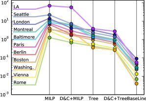
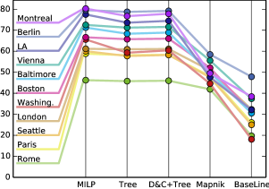
Figure 6: 6 Running times in seconds of the algorithms (logarithmic scale). 6 Percentage of labeled road sections over all zoom levels broken into the different algorithms.

Phase 1. With a maximum of 67 seconds (London, zoom 17) and 27 seconds averaged over all instances, Phase 1 can be applied on large instances in reasonable time. During Phase 1 the number of segments is reduced to between $40\%$ and $83\%$ of the original instance (measured after Step 3, before creating junction edges); see Table 1. This clearly indicates that the procedure aggregates many lanes, since by design the approach does not change the overall geometry, but the simplification maintains the shape of the original network. This is also confirmed by the labelings; see Fig. 1(b)–(c) and interactive maps.

Phase 2, Running Time. We first consider the average running times over all zoom levels; see Fig. 6. We did not measure the running times of Mapnik, because its labeling procedure is strongly interwoven with the remaining rendering procedure, which prevents a fair comparison. As to be expected Milp is the slowest method (max. 126 sec., Los Angeles, ZL 15), while BaseLine is the fastest procedure (max. 0.17 sec.). Combining Milp with D&C results in an average speedup of 2.29 over all instances and a maximum speedup of 3.44; see Table 2.

The algorithm Tree needs less than 4.7 seconds and its median is about 1.3 seconds. Hence, despite its worst-case cubic asymptotic running time, it is fast in practice. Similar to Milp, it is further enhanced by combining it with D&C for a speedup of 1.64 with respect to Tree, and an average speedup of 6.14 with respect to D&C+Milp; see Table 2. In the latter case it has even a maximum speedup of about 21.6. Since decomposing and composing the labelings is done sequentially, the theoretically possible speed up using D&C is not achieved.

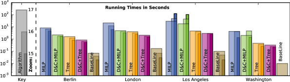
Figure 7: Running times of the algorithms broken down in zoom levels and algorithms. The width of the bars (thin, mediate, wide) corresponds with zoom levels (15, 16, 17).

Figure 8: Decomposition of road networks by D&C. Percentage of long-edges, road sections in paths, trees and other components in which the road networks is decomposed.

If we break down the running times into single zoom levels, we observe similar results; see e.g., Fig. 7. Since with increasing zoom level the instance size grows, for most of the algorithms also the running time increases. Only for North American cities and Milp we observe that the running time for instances of smaller zoom levels are higher than for larger zoom levels.

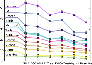
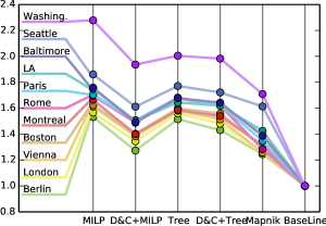
Figure 9: 9 Number of placed labels in thousands. 9 Ratio of labeled road sections and placed labels: ${(\#\text{Labeled Road Sections})}/{(\#\text{Labels})}$.

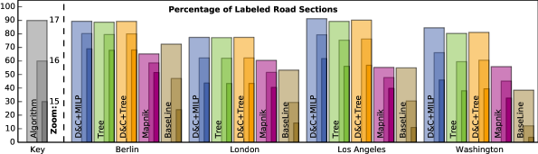
Figure 10: Percentage of labeled road sections broken down in zoom levels and algorithms. The width of the bars (thin, medium, wide) corresponds to the zoom level (15, 16, 17).

Phase 2, Quality. First we analyze the average percentage of labeled road sections over the three zoom levels; see Fig. 6. As an upper bound, Milp, which provably solves MaxLabeledRoads optimally, yields results from $46.2\%$ (Rome) to $80.3\%$ (Montreal). Considering zoom levels independently, we obtain a minimum of $27.5\%$ (Rome, ZL 15) and a maximum of $91.7\%$ (Montreal, ZL 17). We think that the wide span is attributed to the different structures of road networks and road names, e.g., Rome has a lot of short alleys and long road names. Hence, many road components are too short or convoluted to contain a single label. Abbreviating road names could help to overcome this problem.

The algorithm D&C+Tree yields marginally better results than Tree, but only $1\%$ on average, see Table 2. Comparing D&C+Tree with Milp we observe that D&C+Tree yields near-optimal results with respect to our road-section based model. On average it reaches $97\%$ of the optimal solution; see Table 2. While the quality ratio is only $91\%$ for Washington, more than half of the instances are labeled with a quality ratio of $\geq 99\%$. For European cities the percentage of road sections that belong to components that are optimally solved by Tree (long edges, paths, and trees) is notably higher than those for North American cities; see Fig. 8. Nonetheless, we obtain similar percentages of labeled road sections for North American Cities. Hence, the heuristic computing a spanning tree of non-tree components is both fast and yields near-optimal results. The additional implementation effort of Tree is further justified by the observation that the naive way to place labels only on single road sections lags far behind; only $42\%$ on average, $58\%$ as maximum and $24\%$ as minimum compared to the optimal solution. Mapnik achieves on average $75\%$ of the optimal solution and a maximum of $91\%$. For more than the half of the instances Mapnik achieves at most $76\%$ of the optimal solution. So in direct comparison, D&C+Tree labels $31\%$ more road sections than Mapnik on average. Moreover, D&C+Tree has a better utilization of labels and achieves an average ratio of 1.61 labeled road sections per label, compared to Mapnik with a ratio of 1.37; see Fig. 9.

With increasing zoom level the number of labeled road sections is increased, which is to be expected, since more road sections become long-edges; see Fig. 10 for four cities (similar results apply for the others) and Fig. 8. For each zoom level, we observe similar results as described before: Tree and D&C+Tree achieve near-optimal solutions and Mapnik labels considerably fewer road sections. However, for smaller zoom levels the gap between Milp and Mapnik shrinks.

From a visual perspective, labels lie on the skeleton of the road network, which is achieved by design; see Fig. 1(c) and the interactive maps. Instead of unnecessary repetition of labels, labels are only placed if they actually convey additional information. In particular, visual components are labeled, but not single lanes that are indistinguishable due to the zoom level.

6 Conclusion

We introduced a generic framework for labeling road maps based on an abstract road graph model that is combinatorial rather than geometric. We showed in our experimental evaluation that our proposed heuristic for decomposing the road graph into tree-shaped subgraphs and labeling those trees provably optimally is both efficient and effective. It has running times in the range of seconds to one minute even for large road networks such as London with more than 100,000 road sections and achieves near-optimal quality ratios (on average 97%) compared to upper bounds computed by the exact method Milp. Our algorithm clearly outperforms the labeling algorithm of the standard OSM renderer Mapnik, with an average improvement in labeled road sections of $31\%$. Interestingly, Milp is able to compute mathematically optimal solutions within a few minutes for all our test instances, even though it is slower by a factor of about 6 compared to the tree-based algorithm. So for practical purposes there is a trade-off between a final, but rather small improvement in quality at the cost of a significant and by the very nature of Milp unpredictable increase in running time. We only implemented essential cartographic criteria to evaluate the algorithmic core of our framework; further criteria (e.g., abbreviated names) and alternative definitions of road sections can be easily incorporated. The framework can further be pipelined with labeling algorithms for other map features, e.g., after placing labels for point features, one may block all parts of the road network covered by a point label and label the remaining road network such that no labels overlap. While this allows to label different types of features sequentially, constructing a labeling of all features in one single step remains an important open problem.

Acknowledgment. We thank Andreas Gemsa for many interesting and inspiring discussions, and his help on the implementation.

References

- [1] M. Bader and R. Weibel. Detecting and resolving size and proximity con-flicts in the generalization of polygonal maps. In Int. Cartographic Conference (ICC’97), pages 1525–1532, 1997.
- [2] F. Chirié. Automated name placement with high cartographic quality: City street maps. Cartography and Geo. Inf. Science, 27(2):101–110, 2000.
- [3] S. Edmondson, J. Christensen, J. Marks, and S. M. Shieber. A general cartographic labelling algorithm. Cartographica, 33(4):13–24, 1996.
- [4] A. Gemsa, B. Niedermann, and M. Nöllenburg. Label placement in road maps. In V. T. Paschos and P. Widmayer, editors, Algorithms and Complexity (CIAC’15), volume 9079 of LNCS, pages 221–234. Springer, 2015.
- [5] E. Imhof. Positioning names on maps. Amer. Cartogr., pages 128–144, 1975.
- [6] S. Maass and J. Döllner. Embedded labels for line features in interactive 3d virtual environments. In Computer Graphics, Virtual Reality, Visualisation and Interaction (AFRIGRAPH’03), pages 53–59. ACM, 2007.
- [7] G. Neyer and F. Wagner. Labeling downtown. In G. Bongiovanni, R. Petreschi, and G. Gambosi, editors, Algorithms and Complexity (CIAC’00), volume 1767 of LNCS, pages 113–124. Springer, 2000.
- [8] A. Reimer and M. Rylov. Point-feature lettering of high cartographic quality: A multi-criteria model with practical implementation. In EuroCG’14, 2014.
- [9] N. Schwartges, B. Morgan, J.-H. Haunert, and A. Wolff. Labeling streets along a route in interactive 3D maps using billboards. In F. Bacao, M. Y. Santos, and M. Painho, editors, Geo. Inf. Science as an Enabler of Smarter Cities and Communities (AGILE’15), LNGC, pages 269–287. Springer, 2015.
- [10] N. Schwartges, A. Wolff, and J.-H. Haunert. Labeling streets in interactive maps using embedded labels. In Advances in Geographic Information Systems (ACM-GIS’14), pages 517–520. ACM, 2014.
- [11] S. Seibert and W. Unger. The hardness of placing street names in a Manhattan type map. Theor. Comp. Sci., 285:89–99, 2002.
- [12] T. Strijk. Geometric Algorithms for Cartographic Label Placement. Dissertation, Utrecht University, 2001.
- [13] M. Vaaraniemi, M. Treib, and R. Westermann. Temporally coherent real-time labeling of dynamic scenes. In Comput. Geospatial Research Appl. (COM.Geo’12), pages 17:1–17:10. ACM, 2012.
- [14] M. van Kreveld. Geographic information systems. In Handbook of Discrete and Computational Geometry, Second Edition, chapter 58, pages 1293–1314. CRC Press, 2010.
- [15] A. Wolff, L. Knipping, M. van Kreveld, T. Strijk, and P. K. Agarwal. A simple and efficient algorithm for high-quality line labeling. In Innovations in GIS VII: GeoComputation, chapter 11, pages 147–159. Taylor & Francis, 2000.
- [16] A. Wolff and T. Strijk. The map labeling bibliography. http://liinwww.ira.uka.de/bibliography/Theory/map.labeling.html, 2009.