On the semi-classical analysis
of the groundstate energy
of the Dirichlet Pauli operator

Abstract.

We discuss the results of a recent paper by Ekholm, Kovařík and Portmann in connection with a question of C. Guillarmou about the semiclassical expansion of the lowest eigenvalue of the Pauli operator with Dirichlet conditions. We exhibit connections with the properties of the torsion function in mechanics, the exit time of a Brownian motion and the analysis of the low eigenvalues of some Witten Laplacian.

1. Introduction

We study the Dirichlet realization of the Pauli operator $P=(P_{+},P_{-})$,

$$P_{\pm}:=(hD_{x_{1}}-A_{1})^{2}+(hD_{x_{2}}-A_{2})^{2}\pm hB(x)\,,$$

in a bounded, regular and open set $\Omega\subset\mathbb{R}^{2}$. Here $D_{x_{j}}=-i\partial_{x_{j}}$ for $j=1$, $2$. We assume that the magnetic potential $(A_{1},A_{2})$ belongs to $C^{\infty}(\overline{\Omega})^{2}$ and denote by $B(x)=\partial_{x_{1}}A_{2}-\partial_{x_{2}}A_{1}$ the associated magnetic field.

To be more precise, we are interested in the smallest eigenvalue of $P$ as $h\to 0^{+}$. Since the Pauli operator is the square of a Dirac operator this eigenvalue is non-negative. By the diamagnetic inequality it follows that if $B(x)\leq 0$ then the smallest eigenvalue $\lambda_{P_{-}}^{D}(h,B,\Omega)$ of $P_{-}$ satisfies

$$\lambda_{P_{-}}^{D}(h,B,\Omega)\geq h^{2}\lambda^{D}(\Omega).$$ (1.1)

Here $\lambda^{D}(\Omega)$ denotes the smallest eigenvalue of the Dirichlet Laplacian $-\Delta$ in $\Omega$. By symmetry, the same statement holds for $\lambda_{P_{+}}^{D}(h,B,\Omega)$, the smallest eigenvalue of $P_{+}$, in case $B(x)\geq 0$. We will focus our study to the component $P_{-}$ under the assumption

$$\{x\in\Omega:B(x)>0\}\neq\varnothing\,,$$ (1.2)

sometimes with the stronger condition that $B(x)>0$. This means that we cannot directly apply the diamagnetic inequality to conclude the lower bound (1.1). In fact, we will see that $\lambda_{P_{-}}^{D}(h,B,\Omega)$ is exponentially small.

In [10], T. Ekholm, H. Kovařík and F. Portmann give a universal lower bound which can be formulated in the semiclassical context in the following way:

Theorem 1.1 ([10, Theorem 2.1]).

If $B$ does not vanish identically in the simply connected domain $\Omega$ there exists $\epsilon(B,\Omega)>0$ such that, $\forall h>0$,

$$\lambda_{P_{-}}^{D}(h,B,\Omega)\geq\lambda^{D}(\Omega)\,h^{2}\,\exp\bigl{(}-\epsilon(B,\Omega)/h\bigr{)}\,.$$ (1.3)

The proof of the theorem gives a way of computing some upper bound for $\epsilon(B,\Omega)$, by considering the oscillation of scalar potentials $\psi$, i.e. solutions of $\Delta\psi=B$, and optimizing over $\psi$. Although the authors treat interesting examples, they do not give a systematic approach for determining the optimal lower bound.

Scalar potentials will also play a main role for us, and we will fix a canonical one associated with a specific choice of the gauge for the magnetic potential, as used for example in superconductivity theory. Thus, below, $\psi$ will denote the solution of the Poisson problem with Dirichlet boundary condition,

$$\begin{cases}\Delta\psi=B&\text{in $\Omega$}\\ \psi=0&\text{on $\partial\Omega$}.\end{cases}$$ (1.4)

It turns out that this $\psi$ gives the minimal oscillation discussed in [10] under the further condition that $B(x)>0$. In order to answer negatively a question of C. Guillarmou, who was asking for an example for which $B(x)>0$ and there exists $N_{0}$ and $c_{N}>0$ such that $\lambda_{P_{-}}^{D}(h,B,\Omega)\geq c_{N}h^{N}$, we also discuss upper bounds for the ground state energy, and state our main result:

Theorem 1.2.

Assume that $B(x)>0$ in $\Omega$ and that $\psi$ satisfies (1.4). Then

$$\lim_{h\to 0^{+}}h\log\lambda_{P_{-}}^{D}(h,B,\Omega)=2\inf_{\Omega}\psi\,.$$ (1.5)

In particular, this shows that when $B(x)>0$, the optimal $\epsilon(B,\Omega)$ is given by the analysis of (1.4), justifying a posteriori our choice of $\psi$. Moreover, it raises the question on finding $\inf_{\Omega}\psi$. Kawohl proves in [26, 27] that if $\Omega$ is strictly convex and $B(x)$ constant then the infimum is attained at a unique point $x_{0}\in\Omega$. We discuss this, and further properties of $\psi$ in Section 7.

Our lower bound leading to Theorem 1.2 is true for all $h>0$. It is stated and proved in Section 3, see Theorem 3.1.

Under additional assumptions on $\Omega$ or $B(x)$, we will propose a deeper analysis giving more accurate lower bounds or upper bounds and giving in particular the equivalent of $\lambda_{P_{-}}^{D}(h,B,\Omega)$ when $\Omega$ is the disk and $B(x)$ is constant. In fact, we are able to give the main asymptotic term for all exponentially small eigenvalues. This also permits to clarify some miss-statements [20, 14] appearing in the literature and to improve (or correct) the results of [11, 12, 13], [20], [14] and [10].

Theorem 1.3.

Assume that $\Omega=D(0,R)$ is the disk of radius $R$, and that the magnetic field $B(x)$ is constant, $B(x)=B>0$. Let $\lambda^{D}_{P_{-},0}(h)$ denote the smallest eigenvalues of $P_{-}$. Then, as $h\to 0^{+}$,

$$\lambda^{D}_{P_{-},0}(h)=B^{2}R^{2}e^{-BR^{2}/2h}(1+\mathcal{O}(h)).$$ (1.6)

The proof of this theorem, given in Section 5, relies heavily on the rotational symmetry of the ground state which was proven by L. Erdős in [11]. In fact, we make an orthogonal decomposition of $P_{-}$ using angular momentum. The upper bound comes from a very accurate quasimode. For each angular momentum we obtain a spectral gap, enabling us to use the Temple inequality with the quasimode to get also the matching lower bound. It is the lack of this spectral gap that prohibits us to find the corresponding lower bound for general domains $\Omega$.

In Section 6, we recall a statement of L. Erdős permitting in the constant magnetic field case a direct comparison between $\lambda^{D}_{P_{-}}(h,B,\Omega)$ and $\lambda^{D}_{P_{-}}(h,B,D(0,R))$ where $D(0,R)$ is the disk of same area as $\Omega$.

In Section 7 we collect some general properties of the scalar potential $\psi$ in connection with the torsion problem.

We close this introduction with several remarks.

Remark 1.4.

The case $B(x)\leq 0\,$, mentioned above, can be analyzed further under additional conditions (for example, one could think to start with the case when $B(x)$ has a non degenerate negative minimum at a point of $\Omega$). We refer to Helffer–Mohamed [19], Helffer–Morame [20], Helffer–Kordyukov [18] and Raymond–Vu Ngoc [30] for the analysis of the Schrödinger with magnetic field, and note that the addition of the term $-hB(x)$ in $P_{-}$ can be controlled in their analysis.

Remark 1.5.

When $B(x)=2\,$, the solution $\psi$ of (1.4) appears to be $-f_{\tau}$, where $f_{\tau}$ is the so-called torsion function which plays an important role in Mechanics. For this reason there are a lot of treated examples in the engineering literature and a lot of mathematical studies, starting from the fifties with Pólya–Szegö [31]. This permits in particular to improve the applications given in [10].

Remark 1.6.

The problem we study is quite close with the question of analyzing the smallest eigenvalue of the Dirichlet realization of:

$$C_{0}^{\infty}(\Omega)\ni v\mapsto h^{2}\,\int_{\Omega}\left|\nabla v(x)\right|^{2}\;e^{-2f(x)/h}\leavevmode\nobreak\ dx\;.$$

For this case, we can mention Theorem 7.4 in [16], which says (in particular) that, if $f$ has a unique non-degenerate local minimum $x_{min}$, then the lowest eigenvalue $\lambda_{1}(h)$ of the Dirichlet realization $\Delta^{(0)}_{f,h}$ in $\Omega$ satisfies:

$$\lim_{h\rightarrow 0}-h\,\log\lambda_{1}(h)=\inf_{x\in\partial\Omega}(f(x)-f(x_{min}))\;.$$ (1.7)

More precise or general results (prefactors) are given in [6, 7, 21]. This is connected with the semi-classical analysis of Witten Laplacians [36, 22, 23, 8, 32, 17].

Remark 1.7.

It would be interesting to analyze flux effects in the case of a non simply connected domain. We hope to come back to this question in another work.

Acknowledgements

The first author was aware of the question analyzed in [10] at a meeting in Oberwolfach organized in 2014 by V. Bonnaillie-Noël, H. Kovařík and K. Pankrashkin where the authors present their work. He would like to also thank D. Bucur, L. Erdős, C. Guillarmou, and B. Kawohl for useful discussions leading to this paper.

2. Preliminaries

Following what is done for example in superconductivity (see [14]), we can, possibly after a gauge transformation, assume that the magnetic vector potential ${\bf A}=(A_{1},A_{2})$ satisfies

$$\begin{cases}\operatorname{curl}{\bf A}=B\text{ and }\operatorname{div}{\bf A}=0&\text{in $\Omega$}\\ {\bf A}\cdot\nu=0&\text{on $\partial\Omega$}\,.\end{cases}$$ (2.1)

If this is not satisfied for say ${\bf A}_{0}$ satisfying $\operatorname{curl}{\bf A}_{0}=B$, we can construct

$${\bf A}={\bf A}_{0}+\nabla\phi$$

satisfying in addition (2.1), by choosing $\phi$ as a solution of

$$\begin{cases}-\Delta\phi=\operatorname{div}{\bf A}_{0}&\text{ in }\Omega\\ \nabla\phi\cdot\nu=-{\bf A}_{0}\cdot\nu&\mbox{ on }\partial\Omega\,,\end{cases}$$

which is unique if we add the condition $\int_{\Omega}\phi(x)\,dx=0\,$. In this case there exists a scalar potential $\psi$ such that

$$A_{1}=-\partial_{x_{2}}\psi\,,\,A_{2}=\partial_{x_{1}}\psi\,.$$ (2.2)

The condition ${\bf A}\cdot\nu=0\mbox{ on }\partial\Omega$ implies that $\psi=\psi_{i}$ is constant on each connected component $\Gamma_{i}$ of the boundary. Hence, if in addition $\Omega$ is simply connected, there exists a unique $\psi$ such that (2.2) is satisfied and (1.4) holds. In this case, we should write instead

$$\Delta\psi=B\text{ in }\Omega\,,\,\psi=\psi_{i}-\sup\psi_{i}\text{ on }\Gamma_{i}\,.$$ (2.3)

The link with the circulations of ${\bf A}$ along each $\Gamma_{i}$ is analyzed at least formally in [25].

If $B(x)>0$, the minimax principle shows that $\psi\leq 0\,$, and, if $\Omega$ is simply connected, because $B$ is not identically $0$, there exists at least a point $x_{0}\in\Omega$ such that

$$\psi(x_{0})=\inf\psi<0\,.$$ (2.4)

We write

$$\psi_{min}:=\inf\psi\,.$$

In the non simply connected case, the infimum can be attained at one component of the boundary.

3. The lower bound of Ekholm–Kovařík–Portmann revisited.

We come back to the scheme of proof of the lower bound in [10], and state a more explicit bound for positive magnetic fields:

Theorem 3.1.

Assume that $B(x)>0$ in $\Omega\,$. Then

$$\lambda_{P_{-}}^{D}(h,B,\Omega)\geq h^{2}\lambda^{D}(\Omega)\,\exp\Bigl{(}\frac{2\psi_{min}}{h}\Bigr{)}\,.$$ (3.1)

Proof.

We bound the quadratic form from below. Let

$$\Psi=\psi-\psi_{min}\,.$$

Then

$$0\leq\Psi\leq-\psi_{min}\,.$$

We write

$$u=\exp\Bigl{(}-\frac{\Psi}{h}\Bigr{)}\,v\,,$$ (3.2)

and use following identity (see [13] and (2.4) in [10])

$$\langle u,P_{-}u\rangle=h^{2}\int_{\Omega}\exp\Bigl{(}-2\frac{\Psi}{h}\Bigr{)}|(\partial_{x_{1}}+i\partial_{x_{2}})v|^{2}\,dx\,,$$ (3.3)

valid if ${\bf A}$ satisfies (2.1). With $u$ (and consequently $v$) in $H_{0}^{1}(\Omega)$, we get

$$\langle u,P_{-}u\rangle \geq h^{2}\exp\Bigl{(}\frac{2\psi_{min}}{h}\Bigr{)}\int_{\Omega}|(\partial_{x_{1}}+i\partial_{x_{2}})v|^{2}\,dx$$ (3.4)

$$\geq h^{2}\exp\Bigl{(}\frac{2\psi_{min}}{h}\Bigr{)}\int_{\Omega}|\nabla v(x)|^{2}\,dx$$

$$\geq h^{2}\exp\Bigl{(}\frac{2\psi_{min}}{h}\Bigr{)}\lambda^{D}(\Omega)\int_{\Omega}|v(x)|^{2}dx$$

$$\geq h^{2}\exp\Bigl{(}\frac{2\psi_{min}}{h}\Bigr{)}\lambda^{D}(\Omega)\int_{\Omega}|u(x)|^{2}dx\,.$$

Here we have used the Dirichlet condition on $v$ to justify the integration by part in the second step. ∎

Note that the statement is much more explicit than in [10]. It is unclear at this stage that it is accurate (we just make a choice of one $\Psi$ and in [10] there was a minimization over all $\Psi$ satisfying $\Delta\Psi=B$). But note also that our sign condition on the magnetic field is much stronger.

4. Upper bounds in the simply connected case

With the explicit choice of $\psi$ from (1.4), it is straightforward to get:

Proposition 4.1.

Assume that $\Omega$ is simply connected and $B(x)>0$ in $\Omega$. Then, for any $\eta>0\,$, there exists a $C_{\eta}>0$ such that

$$\lambda_{P_{-}}^{D}(h,B,\Omega)\leq C_{\eta}\exp\Bigl{(}\frac{2\psi_{min}}{h}\Bigr{)}\exp\Bigl{(}\frac{2\eta}{h}\Bigr{)}\,.$$ (4.1)

The proof is obtained by taking as trial state $u=\exp\bigl{(}-\frac{\psi}{h}\bigr{)}\,v_{\eta}$, with $v_{\eta}$ compactly supported in $\Omega$ and $v_{\eta}$ being equal to $1$ outside a sufficiently small neighborhood of the boundary and implementing this trial state in (3.3). One concludes by the max-min principle. This proof does not work in the non simply connected case.

The first idea for improvement is to take $\eta=h$ and to control with respect to $h$, but it appears better to consider the trial state

$$u=\exp\Bigl{(}-\frac{\psi}{h}\Bigr{)}-\exp\Bigl{(}\frac{\psi}{h}\Bigr{)}\,.$$ (4.2)

When $\Omega$ is simply connected $u$ evidently satisfies the Dirichlet condition. Using the substitution (3.2),

$$v=1-\exp\Bigl{(}\frac{2\psi}{h}\Bigr{)}\,.$$

Thus,

$$\frac{h^{2}\int_{\Omega}\exp\bigl{(}-\frac{2\psi}{h}\bigr{)}|(\partial_{x_{1}}+i\partial_{x_{2}})v|^{2}\,dx}{\int_{\Omega}\exp\bigl{(}-\frac{2\psi}{h}\bigr{)}|v|^{2}\,dx} =4\frac{\int_{\Omega}\exp\bigl{(}\frac{2\psi}{h}\bigr{)}|(\partial_{x_{1}}+i\partial_{x_{2}})\psi|^{2}\,dx}{\int_{\Omega}\exp\bigl{(}-\frac{2\psi}{h}\bigr{)}|v|^{2}\,dx}$$

$$=4\frac{\int_{\Omega}\exp\bigl{(}\frac{2\psi}{h}\bigr{)}|\nabla\psi|^{2}\,dx}{\int_{\Omega}\exp\bigl{(}-\frac{2\psi}{h}\bigr{)}|v|^{2}\,dx}$$

$$=2h\frac{\int_{\Omega}\bigl{(}\nabla\exp\bigl{(}\frac{2\psi}{h}\bigr{)}\bigr{)}\cdot\nabla\psi\,dx}{\int_{\Omega}\exp\bigl{(}-\frac{2\psi}{h}\bigr{)}|v|^{2}\,dx}$$

We integrate by parts in the numerator,

$$\int_{\Omega}\Bigl{(}\nabla\exp\Bigl{(}\frac{2\psi}{h}\Bigr{)}\Bigr{)}\cdot\nabla\psi\,dx =\int_{\partial\Omega}\nu\cdot\nabla\psi-\int_{\Omega}\exp\Bigl{(}\frac{2\psi}{h}\Bigr{)}B(x)\,dx$$ (4.3)

$$=\int_{\Omega}B(x)\,dx-\int_{\Omega}\exp\Bigl{(}\frac{2\psi}{h}\Bigr{)}B(x)\,dx$$

$$\leq\int_{\Omega}B(x)\,dx\,.$$

In the simply connected case, we know by Hopf Lemma that $\nu\cdot\nabla\psi$ does not vanish at the boundary. This implies, using the Laplace integral method in a tubular neighborhood of the boundary, that

$$\int_{\Omega}\exp\Bigl{(}\frac{2\psi}{h}\Bigr{)}B(x)\,dx=\mathcal{O}(h)\,.$$

This suggests that the upper bound in (4.3) is rather sharp, but we will not use this property.

We turn to the denominator. In case there is a unique point $x_{0}\in\Omega$ where $\psi$ attains its minimum, we have the following lower bound, for some $\epsilon>0$,

$$\int_{\Omega}\exp\Bigl{(}-\frac{2\psi}{h}\Bigr{)}|v|^{2}\,dx \geq\int_{D(x_{0},\epsilon)}\exp\Bigl{(}-\frac{2\psi}{h}\Bigr{)}|v|^{2}\,dx$$ (4.4)

$$\sim\exp\Bigl{(}\frac{-2\psi_{min}}{h}\Bigr{)}\int_{D(x_{0},\epsilon)}\exp\Bigl{(}-\frac{2(\psi(x)-\psi_{min})}{h}\Bigr{)}\,dx\,.$$

If there are a finite number $N$ of points $x_{j}$ in $\Omega$ such that $\psi(x_{j})=\psi_{min}$,

$$\int_{\Omega}\exp\Bigl{(}-\frac{2\psi}{h}\Bigr{)}|v|^{2}\,dx \geq\sum_{j=1}^{N}\int_{D(x_{j},\epsilon)}\exp\Bigl{(}-\frac{2\psi}{h}\Bigr{)}|v|^{2}\,dx$$ (4.5)

$$\sim\sum_{j=1}^{N}\exp\Bigl{(}\frac{-2\psi_{min}}{h}\Bigr{)}\int_{D(x_{j},\epsilon)}\exp\Bigl{(}-\frac{2(\psi(x)-\psi_{min})}{h}\Bigr{)}\,dx\,,$$

where $\epsilon>0$ is chosen such that the balls $D(x_{j},\epsilon)$ are disjoint.

If $\operatorname{Hess}\psi(x_{j})$ is positive, using the Laplace integral method, we get

$$\int_{D(x_{j},\epsilon)}\exp\Bigl{(}-\frac{2(\psi(x)-\psi_{min})}{h}\Bigr{)}\,dx\sim\pi h(\det(\operatorname{Hess}\psi(x_{j})))^{-\frac{1}{2}}\,.$$ (4.6)

If $\operatorname{Hess}\psi(x_{j})$ is not positive definite, then it necessarily has one zero eigenvalue and the other one equals $B(x_{j})$. After a change of variable, we can assume that, with $x_{j}=(x_{j1},x_{j2})$, there exists $C_{\epsilon}$ such that

$$\psi(x,y)-\psi_{min}\leq C_{\epsilon}((x-x_{j1})^{2}+(y-x_{j2})^{4})\,,\,\text{ in }D(x_{j},\epsilon)\,.$$

In this case we get, the existence of $d_{\epsilon}>0$ such that, as $h\to 0\,$,

$$\int_{D(x_{j},\epsilon)}\exp\Bigl{(}-\frac{2(\psi(x)-\psi_{min})}{h}\Bigr{)}\,dx\geq d_{\epsilon}h^{\frac{3}{4}}.$$ (4.7)

This leads us to consider two cases:

1. For all the $x_{j}$ such that $\psi(x_{j})=\psi_{min}$, $\operatorname{Hess}\psi(x_{j})$ positive definite.

2. There exists $x_{0}$ such that $\psi(x_{0})=\psi_{min}$ and $\operatorname{Hess}\psi(x_{0})$ is degenerate.

Note that Case 1 contains the case when $\Omega$ is convex and $B(x)=B>0$. In this case there is a unique $x_{j}$ (see Proposition 7.1 below).

The lower bounds in (4.4) and (4.5) together with the upper bound deduced from (4.3) lead to the following upper bounds.

Theorem 4.2.

Assume that $\Omega$ is simply connected and that $B(x)>0$ in $\Omega$. Denote by $\Phi=\frac{1}{2\pi}\int_{\Omega}B(x)\,dx$ the flux of the magnetic field $B(x)$ through $\Omega$.

1. In case 1, as $h\to 0^{+}$,

   $$\lambda_{P_{-}}^{D}(h,B,\Omega)\leq 4\Phi\,\biggl{[}\sum_{j=1}^{N}\left(\det\,(\operatorname{Hess}\psi(x_{j}))\right)^{-\frac{1}{2}}\,\biggr{]}^{-1}\exp\Bigl{(}\frac{2\psi_{min}}{h}\Bigr{)}(1+o(1))\,.$$ (4.8)

2. In case 2, as $h\to 0^{+}$,

   $$\lambda_{P_{-}}^{D}(h,B,\Omega)=\mathcal{O}(h^{\frac{1}{4}})\exp\Bigl{(}\frac{2\psi_{min}}{h}\Bigr{)}\,.$$ (4.9)

In the case of the disk $D(0,R)$, we get, as $h\to 0^{+}\,$,

$$\lambda_{P_{-}}^{D}(h,B,D(0,R))\leq B^{2}R^{2}\exp(-BR^{2}/2h)(1+o(1))\,.$$ (4.10)

We will see in Section 5 that it is optimal for the disk. Unfortunately, the proof is specific of the disk.

Remark 4.3.

• When $\Omega$ is not simply connected, we can use the domain monotonicity of the Dirichlet problem and apply the previous result for any simply connected domain $\widetilde{\Omega}$ contained in $\Omega$. The natural question is then to find the optimal domain and it is unclear if this would lead to the optimal decay.

• The same monotonicity argument could be used for treating the case when $B$ is changing sign. We should add in this case for the choice of $\widetilde{\Omega}$ the condition that $B>0$ on $\widetilde{\Omega}$.

5. The case of the disk in the constant magnetic case revisited.

In this section we work with constant magnetic field $B(x)=B>0$ in the disk $\Omega=D(0,R)$, and our aim is to prove Theorem 1.3. We actually present a more general analysis of the spectrum.

We introduce polar coordinates $(r,\theta)$ via $x_{1}=r\cos\theta$ and $x_{2}=r\sin\theta$. As is well-known, the variables separate, and we are led to study the infinite family of operators $\mathcal{P}_{m}(h)$, $m\in\mathbb{Z}$, where

$$\mathcal{P}_{m}(h)=h^{2}\Bigl{[}-\frac{d^{2}}{dr^{2}}-\frac{1}{r}\frac{d}{dr}+\Bigl{(}\frac{m}{r}-\frac{Br}{2h}\Bigr{)}^{2}\Bigl{]}-hB.$$

The spectrum of $P_{-}$ is the union of the spectrum of the operators $\mathcal{P}_{m}(h)$.

Theorem 5.1.

For $m\in\mathbb{Z}$, let $\lambda_{m,0}^{D}(h)\leq\lambda_{m,1}^{D}(h)\leq\ldots$ denote the increasing sequence of eigenvalues of $\mathcal{P}_{m}(h)$.

1. If $m<0$ then $\lambda_{m,0}^{D}(h)\geq(2|m|-1)hB\,$.

2. If $m\geq 0$ then $\lambda_{m,k}^{D}(h)\geq 2hBk\,$.

   In particular, the second eigenvalue satisfies $\lambda_{m,1}^{D}(h)\geq 2hB\,$.

3. If $m\geq 0$, then, as $h\to 0^{+}\,$,

   $$\lambda_{m,0}^{D}(h)=2hB\frac{(BR^{2}/2h)^{m+1}}{m!}e^{-BR^{2}/2h}(1+O(h))\,.$$

Proof of Theorem 1.3.

We know from [11] that the lowest eigenvalue comes from the angular momentum $m=0$, i.e. $\lambda_{P_{-},0}^{D}(h)=\lambda_{0,0}^{D}(h)$. Thus, the result in Theorem 1.3 is a direct consequence of statement c in Theorem 5.1. ∎

Proof of Theorem 5.1.

We divide the proof into several steps.

Proof of a

This follows directly from an estimate of the potential,

$$h^{2}\Bigl{(}\frac{m}{r}-\frac{Br}{2h}\Bigr{)}^{2}=\Bigl{(}\frac{hm}{r}\Bigr{)}^{2}+\Bigl{(}\frac{Br}{2}\Bigl{)}^{2}-mhB\geq 2|m|hB\,,$$

and a comparison of quadratic forms.

Proof of b

We will use the fact that the eigenfunctions of $\mathcal{P}_{m}$ can be expressed in terms of Kummer functions together with a result on zeros of these functions, explained below.

The Kummer differential equation reads

$$z\frac{d^{2}w}{dz^{2}}+(b-z)\frac{dw}{dz}-aw=0\,.$$

One solution to Kummer’s equation, that is regular at $z=0\,$, is given by

$$\mathbf{M}(a,b,z)=\sum_{s=0}^{+\infty}\frac{(a)_{s}}{\Gamma(b+s)}z^{s}\,.$$

Here $(a)_{s}$ denotes the Pochhammer symbol, $(a)_{0}=1$ and

$$(a)_{s}=a(a+1)\cdots(a+s-1)\quad\text{for $s\geq 1\,$.}$$

It follows that a solution $u$ to the eigenvalue equation $\mathcal{P}_{m}u=\lambda u\,$, that is regular at $r=0\,$, is given by

$$u(r)=e^{-Br^{2}/4h}r^{m}\,\mathbf{M}\Bigl{(}-\frac{\lambda}{2hB},m+1,\frac{Br^{2}}{2h}\Bigr{)}\,.$$

Since we are interested in the Dirichlet case, the eigenvalues are determined by the condition $u(R)=0\,$, giving us the equation

$$\mathbf{M}\Bigl{(}-\frac{\lambda}{2hB},m+1,\frac{BR^{2}}{2h}\Bigr{)}=0\,.$$ (5.1)

Thus, given $b\in\mathbb{N}\setminus\{0\}$ we are interested in zeros of $a\mapsto\mathbf{M}(a,b,z)$ for large positive $z$.

Lemma 5.2 ([29, §13.9]).

Let $p(a,b)$ denote the number of positive zeros to the function $\mathbb{R}\ni z\mapsto\mathbf{M}(a,b,z)\,$. Then

1. $p(a,b)=0$ if $a\geq 0$ and $b\geq 0\,$.

2. $p(a,b)=\lceil-a\rceil$ if $a<0$ and $b\geq 0\,$. Here $\lceil x\rceil$ denotes the smallest integer greater than or equal to $x$.

It follows that the equation (5.1) has no solutions for $\lambda<0$ (which we already know, since $P_{-}$ is non-negative) and at most $k$ solutions in the interval $0<\lambda<2khB$. We conclude that $\lambda_{m,k}^{D}(h)\geq 2khB$.

Proof of the upper bound in c

We work here with $\mathcal{P}_{m}$ , $m\geq 0\,$. We will use as trial state

$$v(r)=r^{m}\bigl{(}e^{BR^{2}/4h-Br^{2}/4h}-e^{Br^{2}/4h-BR^{2}/4h}\bigr{)}.$$

A calculation shows that, as $h\to 0^{+}\,$,

$$\|v\|^{2}=\int_{0}^{R}v(r)^{2}\,r\,dr=2^{m}m!\Bigl{(}\frac{h}{B}\Bigr{)}^{m+1}e^{BR^{2}/2h}+\mathcal{O}(1)$$

and

$$\mathcal{P}_{m}v=2(m+1)hBr^{m}e^{Br^{2}/4h-BR^{2}/4h}\,.$$ (5.2)

Multiplying $\mathcal{P}_{m}v$ with $v$ and integrating we find that, as $h\to 0^{+}$,

$$\langle v,\mathcal{P}_{m}(h)v\rangle=hBR^{2(m+1)}+\mathcal{O}(h^{2})\,.$$

This gives the lower bound, as $h\to 0^{+}\,$,

$$\lambda_{m,0}^{D}(h)\leq\frac{\langle v,\mathcal{P}_{m}(h)v\rangle}{\|v\|^{2}}=\frac{2hB(BR^{2}/2h)^{m+1}}{m!}e^{-BR^{2}/2h}(1+\mathcal{O}(h))\,.$$

Proof of the lower bound in c

We will use the Temple inequality, saying that

$$\lambda_{m,0}^{D}(h)\geq\eta-\frac{\epsilon^{2}}{\beta-\eta}\,,$$

with

$$\eta=\frac{\langle v,\mathcal{P}_{m}(h)v\rangle}{\|v\|^{2}},\quad\epsilon^{2}=\frac{\|\mathcal{P}_{m}v\|^{2}}{\|v\|^{2}}-\eta^{2},\quad\beta=2hB\leq\lambda_{m,1}^{D}(h)\,.$$

From (5.2) we get

$$\|\mathcal{P}_{m}v\|^{2}=4(1+m)^{2}h^{3}BR^{2m}(1+\mathcal{O}(h))\,.$$

From the lower bound of the second eigenvalue, we take $\beta=2hB$. Hence, if $h$ is sufficiently small,

$$\frac{1}{\beta-\eta}=\frac{1}{2hB}(1+\mathcal{O}(h^{+\infty})).$$

In $\epsilon^{2}$ the term $\eta^{2}$ is negligible in comparison with the first term. Thus, as $h\to 0^{+}\,$,

$$\frac{\epsilon^{2}}{\beta-\eta}=\frac{2h}{BR^{2}}(1+m)^{2}\frac{2hB(BR^{2}/2h)^{m+1}}{m!}e^{-BR^{2}/2h}(1+\mathcal{O}(h))\,.$$

Thus, compared with $\eta$ this term has an extra power of $h$, and thus can be considered as an error term, and we get the lower bound as $h\to 0^{+}$

$$\lambda_{m,0}^{D}(h)\geq\frac{2hB(BR^{2}/2h)^{m+1}}{m!}e^{-BR^{2}/2h}(1+\mathcal{O}(h))\,.$$ (5.3)

This completes the proof of Theorem 5.1. ∎

Remark 5.3.

In fact, the calculations in the proof of Theorem 5.1 suggest that if $\lambda^{D}_{P_{-},0}(h)\leq\lambda^{D}_{P_{-},1}(h)\leq\cdots$ denotes the increasing sequence of eigenvalues of $P_{-}$ then

$$\lambda^{D}_{P_{-},m}(h)=2hB\frac{(BR^{2}/2h)^{m+1}}{m!}e^{-BR^{2}/2h}(1+\mathcal{O}(h))\,.$$

This would have given an alternative proof of Erdős’s result [11] but the uniform control in $m$ is missing in the estimates given by Theorem 5.1.

6. A Faber-Krahn type Erdős inequality

We recall one by L. Erdős ([11, 12]) which is useful in this context.

Proposition 6.1.

For any planar domain $\Omega$ and $B>0$, let $\lambda^{D}(h,B,\Omega)$ be the ground state energy of the Dirichlet realization of the semi-classical magnetic Laplacian with constant magnetic field equal to $B$ in $\Omega$. Then we have:

$$\lambda^{D}(h,B,\Omega)\geq\lambda^{D}(h,B,D(0,R))\;,$$ (6.1)

where $D(0,R)$ is the disk with same area as $\Omega\,$:

$$\pi R^{2}=\operatorname{Area}(\Omega)\,.$$

Moreover the equality in (6.1) occurs if and only if $\Omega=D(0,R)\,$.

Hence we can combine this proposition with the optimal lower bound obtained for the disk (with $m=0$).

7. Properties of the scalar potential—the torsion problem

In this section, we revisit a discussion of [10] about relating the decay rate with either the geometry of $\Omega$ or the properties of the magnetic field. We would like to see if the fact that we have the optimal $\psi_{min}$ can lead to the improvements of the statements of [10] by using classical results in the theory of the torsion function. In this section we assume that $B(x)=1$, so $-2\psi=f_{\tau}$ is the torsion function in $\Omega$, for which we collect available upper bounds. Our main reference is the book by R. Sperb [34].

7.1. Saint–Venant torsion problem and application

We refer here to Example 3.4 in [27]. Let $\Omega\subset\mathbb{R}^{n}$ be a strictly convex domain and let $f_{\tau}$ be the solution of the Saint–Venant torsion problem

$$\begin{cases}\Delta f_{\tau}=-2&\text{ in }\Omega\\ f_{\tau}=0&\text{ on }\partial\Omega.\end{cases}$$ (7.1)

The function $f_{\tau}$ is also known as warping function. For $n=2$ it is known from [26] that the square root of $f_{\tau}$ is a strictly concave function. For $n\geq 2$ the concavity follows from Lemma 3.12 and Theorem 3.13 in [27]. As a consequence, we get

Proposition 7.1.

If $\Omega$ is strictly convex and $B(x)=1$, then there exists a unique $x_{0}$ such that $\psi(x_{0})=\psi_{min}$ .

Note that at $x_{0}$, the Hessian of $\psi$ is definite positive. This can be deduced from the information on $f_{\tau}=-2\psi$ given by Kawohl’s result. At $x_{0}$, we have indeed

$$\operatorname{Hess}\psi(x_{0})=-f_{\tau}^{\frac{1}{2}}(x_{0})\,\operatorname{Hess}f_{\tau}^{\frac{1}{2}}(x_{0})\,,$$

and the trace of the Hessian of $\psi$ at $x_{0}$ is positive.

If $\Omega$ is not convex, we can loose the uniqueness of $x_{0}$ as for example in the case of the dumbell (see Figure 7.1).

Figure 7.1. Levels of $\psi$ in the case of the dumbell.

Remark 7.2.

• Some literature in Mechanics (see for example [15]) claims the concavity of the torsion function $f_{\tau}$ in the strictly convex case (at least when $f_{\tau}$ is a polynomial) but this is obviously wrong in the case of the equilateral triangle (see next subsection).

• It is natural to ask the same question for solutions of $\Delta u=-2B(x)$ for $B>0$ non-constant. We have no condition on $B$ to propose implying the uniqueness for the maximum of $u$. We have only verified that the argument given in [27] in the case of constant $B$ breaks down as soon as $B$ is not constant.

7.2. Examples

Below we discuss the situation in some simple domains. We refer to [15] for many other examples of domains for which explicit (or semi-explicit) computations can be done. In Figure 7.2, we show the level sets obtained for $\psi$ using Mathematica.

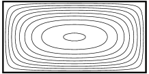
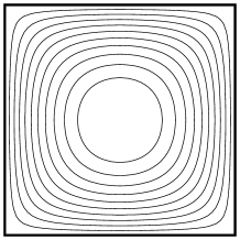
Figure 7.2. Levels of $\psi$ in the case of the ellipse, rectangle, square and triangle.

7.2.1. The disk

If $\Omega=D(0,1)$ and $B=1$, we have

$$\psi(x)=\frac{1}{4}|x|^{2}-\frac{1}{4}\,,\quad\psi_{min}=-\frac{1}{4}\,.$$ (7.2)

Theorem 3.1 gives a rather accurate lower bound but see Section 5 for the optimal result.

7.2.2. The ellipse

If $\Omega=\bigl{\{}(x,y)\in\mathbb{R}^{2}\,,\,\frac{x^{2}}{a^{2}}+\frac{y^{2}}{b^{2}}<1\bigr{\}}$. then, for $B=1\,$,

$$\psi(x,y)=\frac{1}{2/a^{2}+2/b^{2}}\,\Bigl{(}\frac{x^{2}}{a^{2}}+\frac{y^{2}}{b^{2}}-1\Bigr{)}\,,\quad\psi_{min}=-\frac{1}{2/a^{2}+2/b^{2}}\,.$$ (7.3)

7.2.3. The rectangle

For the rectangle $(-\frac{a}{2},\frac{a}{2})\times(-\frac{b}{2},\frac{b}{2})$, we have an explicit solution using Fourier series (see [15] or this course):

$$\psi_{a,b}(x,y)=-\sum_{(k,\ell)\in\mathbb{N}_{odd}^{2}}\frac{(-1)^{\frac{k+\ell}{2}-1}2^{4}a^{2}b^{2}}{\pi^{4}k\ell(k^{2}b^{2}+\ell^{2}a^{2})}\,\cos\frac{k\pi x}{a}\,\cos\frac{\ell\pi y}{b}.$$ (7.4)

In the case of the square (with $a=b=2$) one has $\psi_{2,2}(0,0)\approx-0.294685$. In the limit $b\to+\infty$ one recovers the argument of [10], who use the function $\psi$ corresponding to the band of size $a$:

$$\psi_{a,\infty}(x)=\frac{1}{2}\Bigl{(}x^{2}-\Bigl{(}\frac{a}{2}\Bigr{)}^{2}\Bigr{)}\,,\quad\psi_{a,\infty,min}=-\frac{a^{2}}{8}\,.$$

7.2.4. The equilateral triangle

For the equilateral triangle, there is an explicit formula given by

$$\psi(x,y)=-\frac{1}{4a}\,\Bigl{(}x-\sqrt{3}y-\frac{2}{3}a\Bigr{)}\Bigl{(}x+\sqrt{3}y-\frac{2}{3}a\Bigr{)}\Bigl{(}x+\frac{1}{3}a\Bigr{)}\,,\quad\psi_{min}=-\frac{a^{2}}{27}\,,$$ (7.5)

the minimum of $\psi$ is attained at $(0,0)$ .

7.3. Known bounds for the torsion function

The problem of the torsion of an elastic beam is explained in [34, p. 3]. But the main properties are analyzed in Chapter 6 (mainly Section 6.1). For a given $\Omega$, we can define the diameter $\delta(\Omega)$, the maximal width $\ell(\Omega)$ and the inner radius $\rho(\Omega)$. We have the following estimates:

$$\psi_{min} \geq-\frac{\delta(\Omega)^{2}}{4}\,,$$ (7.6)

$$\psi_{min} \geq-\frac{\ell(\Omega)^{2}}{8}\,,$$ (7.7)

and, in the convex case,

$$\psi_{min} \geq-\frac{\rho(\Omega)^{2}}{2}\,.$$ (7.8)

Inequality (7.7) permits to recover the result of [10] and (7.8) in the convex case is better than the corresponding statement in [10]. There are more accurate estimates, when $\Omega$ has two axes of symmetry, see equation (6.14) in [34].

It is also interesting to mention the inequality due, according to the book of R. Sperb [34, p. 193], to Pólya–Szegö [31] (1951):

$$\psi_{min}(\Omega)\geq\psi_{min}(D(0,R))\,,$$ (7.9)

where $R$ is the radius of the disk of same area as $\Omega$. This result is coherent with the Erdős result recalled in Proposition 6.1.

7.4. General comparison statements for $\psi_{min}$

In order to have lower bounds or upper bounds for $\psi_{min}$, one way, using the maximum principle, is to either find $\psi^{sub}$ such that

$$\Delta\psi^{sub}\geq B\text{ in }\Omega\,;\,\psi^{sub}\leq 0\text{ on }\partial\Omega\,,$$ (7.10)

which will imply

$$\psi^{sub}_{min}\leq\psi_{min}\,,$$ (7.11)

or to find $\psi^{sup}$

$$\Delta\psi^{sup}\leq B\text{ in }\Omega\,;\,\psi^{sup}\geq 0\text{ on }\partial\Omega\,,$$ (7.12)

which will imply

$$\psi^{sup}_{min}\geq\psi_{min}.$$ (7.13)

This can be used in different ways:

• In the case, when $B(x)>0$, use the comparison between the magnetic field $B(x)$ and the constant magnetic field $\inf B$ and $\sup B$.

• Recover Theorem 2.2 in [10] but (7.7) is more direct.

Note that this gives for $\psi_{min}$ a monotonicity result with respect to $B$ which is not necessarily true for the Pauli operator itself.

7.5. The results by C. Bandle

In [2] C. Bandle uses isoperimetric techniques and the conformal mapping theorem. The domain $\Omega$ is supposed to be simply connected and $B>0$ is supposed to satisfy

$$\Delta\log B(x)+2CB(x)\geq 0\quad\text{in }\overline{\Omega}$$

for some constant $C\in\mathbb{R}\,$. If $u$ solves

$$\begin{cases}\Delta u=-B(x)&\text{in $\Omega$}\\ u=0&\text{on $\partial\Omega$}\,,\end{cases}$$

and if $CM<4\pi$, where $M=\int_{\Omega}B(x)\,dx$ is the flux of the magnetic field, then $u$ satisfies the bound

$$u(x)\leq\frac{1}{C}\log\frac{4\pi}{4\pi-CM}\,.$$

with equality when $\Omega$ is the disk, and $B(x)=(1+C|x|^{2}/4)^{-2}$ (or a situation conformally equivalent to this). When $C=0$, the result reads

$$u(x)\leq\frac{M}{4\pi}\,,$$

and we recover (7.9) in the case $B>0$ constant.

In [33, 35] one can find other estimates, involving curvature terms.

7.6. Torsion, lifetime and Hardy inequality

In the twodimensional case, one should also mention (see [3, Theorem 1]) the following estimates:

Proposition 7.3.

Let us assume that $\Omega$ is simply connected in $\mathbb{R}^{2}$. With $\psi$ solution of $\Delta\psi=1$ in $\Omega$, $\psi_{/\partial\Omega}=0$, we have

$$\lambda(\Omega)^{-1}\leq|\psi_{min}|\leq\frac{7\zeta(3)}{16}{\bf j}^{2}\lambda(\Omega)^{-1}\,.$$ (7.14)

Note that

$$\frac{7\zeta(3)}{16}{\bf j^{2}}<0.5259\times{\bf j}^{2}<0.5259\times 5.784025<3.0419\,.$$

One can then combine with Hardy’s inequality (see [1, 3, 4, 9, 28, 5, 24]) but this does not seem to give significative improvements in our twodimensional situation when we compare with what is given by (7.7) or (7.8). $|\psi_{min}|$ is also related to the maximal expected lifetime of a Brownian motion (see [3, 4]).

References

- [1] A. Ancona. On strong barriers and inequality of Hardy for domains in . J. London Math. Soc. 2 (34), 274–290 (1986).
- [2] C. Bandle. Bounds for the solution of Poisson problems and applications to nonlinear eigenvalue problems. SIAM J. Math. Anal. 6, 146–152 (1975).
- [3] R. Bañuelos, T. Carroll. Brownian motion and the fundamental frequency of a drum. Duke Mathematical Journal 75, 575–602 (1994).
- [4] R. Bañuelos, T. Carroll. The maximal expected lifetime of Brownian motion. Mathematical Proc. Royal Irish Acad. 111A, 1–11 (2011).
- [5] M. van den Berg and T. Carroll. Hardy inequality and estimates for the torsion function, Bull. London Math. Soc. 41, 980–986 (2009).
- [6] A. Bovier, M. Eckhoff, V. Gayrard, and M. Klein : Metastability in reversible diffusion processes I: Sharp asymptotics for capacities and exit times. JEMS 6(4), 399–424 (2004).
- [7] A. Bovier, V. Gayrard, and M. Klein. Metastability in reversible diffusion processes II: Precise asymptotics for small eigenvalues. JEMS 7(1), 69–99 (2004).
- [8] H.L Cycon, R.G Froese, W. Kirsch, and B. Simon. Schrödinger operators with application to quantum mechanics and global geometry. Text and Monographs in Physics. Springer Verlag (1987).
- [9] E.B. Davies. Spectral theory and differential operators. Cambridge studies in Advanced Maths. 42. Cambridge University Press 1995.
- [10] T. Ekholm, H. Kovařík, and F. Portmann. Estimates for the lowest eigenvalue of magnetic Laplacians. J. Math. Anal. Appl. 439, 330–346 (2016).
- [11] L. Erdős. Rayleigh-type isoperimetric inequality with a homogeneous magnetic field. Calc. Var. 4 (1996) 283–292.
- [12] L. Erdős. Lifschitz tail in a magnetic field: the nonclassical regime. Probab. Theory Relat. Fields 112 321–371.
- [13] L. Erdős and V. Vougalter. Pauli operator and Aharonov–Casher theorem for measure valued magnetic fields. Comm. Math. Phys. 225, 399–421 (2002).
- [14] S. Fournais and B. Helffer. Spectral methods in surface superconductivity. Progress in Nonlinear Differential Equations and Their Applications 77 (2010).
- [15] J. Francu, P. Novackova, and P. Janicek. Torsion of a non-circular bar. Engineering Mechanics, Vol. 19, No. 1, 45–60 (2012).
- [16] M.I. Freidlin and A.D. Wentzell. Random perturbations of dynamical systems. Transl. from the Russian by Joseph Szuecs. 2nd ed. Grundlehren der Mathematischen Wissenschaften. 260. New York (1998).
- [17] B. Helffer, M. Klein and F. Nier. Quantitative analysis of metastability in reversible diffusion processes via a Witten complex approach. Matematica Contemporanea, 26, 41–85 (2004).
- [18] B. Helffer and Y. A. Kordyukov. Accurate semiclassical spectral asymptotics for a two-dimensional magnetic Schrödinger operator. Annales Henri Poincaré, 16 (7), 1651–1688 (2015).
- [19] B. Helffer and A. Mohamed. Semiclassical analysis for the ground state energy of a Schrödinger operator with magnetic wells. J. Funct. Anal. 138 (1), 40–81 (1996).
- [20] B. Helffer and A. Morame. Magnetic bottles in connection with superconductivity. J. Funct. Anal. 185, 604–680 (2001).
- [21] B. Helffer and F. Nier. Quantitative analysis of metastability in reversible diffusion processes via a Witten complex approach: the case with boundary. Mém. Soc. Math. Fr. (N.S.) No. 105 (2006).
- [22] B. Helffer and J. Sjöstrand. Multiple wells in the semi-classical limit I, Comm. Partial Differential Equations 9 (4), 337–408 (1984).
- [23] B. Helffer and J. Sjöstrand. Puits multiples en limite semi-classique IV -Etude du complexe de Witten -. Comm. Partial Differential Equations 10 (3), 245–340 (1985).
- [24] J. Hersch. Sur la fréquence fondamentale d’une membrane vibrante: évaluations par défaut et principe du maximum. Z. Angew. Math. Mech. 11, 387–413 (1960).
- [25] T.F. Jablonski and H. Andreaus. Torsion of a Saint-Venant cylinder with a nonsimply connected cross-section. Engineering Transactions 47 (1), 77–91, (1999).
- [26] B. Kawohl. When are superharmonic functions concave? Applications to the St. Venant torsion problem and to the fundamental mode of the clamped membrane. Z. Angew. Math. Mech. 64, 364–366 (1984).
- [27] B. Kawohl. Rearrangements and convexity of level sets in PDE. Lecture Notes in. Mathematics 1150. Springer (1985).
- [28] A. Laptev and A. V. Sobolev. Hardy inequalities for simply connected planar domains. arXiv:math/0603362.
- [29] A. B. Olde Daalhuis. Confluent hypergeometric functions. NIST handbook of mathematical functions. U.S. Dept. Commerce, Washington, DC, 321–349 (2010).
- [30] N. Raymond, S. Vũ Ngọc. Geometry and Spectrum in 2D Magnetic Wells. Annales de l’institut Fourier. 65 (1), 137–169 (2015).
- [31] G. Pólya and G. Szegö. Isoperimetric Inequalities in Mathematical Physics. Princeton University Press, Princeton, New Jersey (1951).
- [32] B. Simon. Semi-classical analysis of low lying eigenvalues, I.. Nondegenerate minima: Asymptotic expansions. Ann. Inst. H. Poincaré Phys. Théor. 38, p. 296–307 (1983).
- [33] P.W. Schaefer and R.P. Sperb. Maximum principles and bounds in some inhomogeneous elliptic boundary value problems. SIAM J. Math. Anal. 8, 871–878 (1977).
- [34] R. Sperb. Maximum principles and their applications. Academic Press, New York, 1981.
- [35] R. Sperb. Maximum principles and nonlinear elliptic problems. J. d’Analyse Mathématique, Vol. 35, 236–263 (1979).
- [36] E. Witten. Supersymmetry and Morse inequalities. J. Diff. Geom. 17, 661–692 (1982).