Investigating the origin of hot gas lines in Herbig Ae/Be Stars

Abstract

We analyze high–resolution UV spectra of a small sample of Herbig Ae/Be stars (HAEBES) in order to explore the origin of the $T\sim 10^{5}$ K gas in these stars. The C IV 1548,1550 Å line luminosities are compared to non–simultaneous accretion rate estimates for the objects showing C IV emission. We show that the correlation between $L_{CIV}$ and $\dot{M}$ previously established for classical T Tauri stars (CTTSs) seems to extend into the HAEBE mass regime, although the large spread in literature $\dot{M}$ and $A_{V}$ values makes the actual relationship highly uncertain. With the exception of DX Cha, we find no evidence for hot, optically thick winds in our HAEBE sample. All other objects showing clear doublet emission in C IV can be well described by a two component (i.e., a single component for each doublet member) or four component (i.e., two components for each doublet member) Gaussian emission line fit. The morphologies and peak-flux velocities of these lines suggest they are formed in weak, optically thin stellar winds and not in an accretion flow, as is the case for the hot lines observed in CTTSs. The lack of strong outflow signatures and lack of evidence for line formation in accretion flows is consistent with the conclusion presented in our recent optical and He I 10830 Å studies that the immediate circumstellar environments of HAEBES, in general, are not scaled–up analogs of the immediate environments around CTTSs. The conclusions presented here for hot gas lines around HAEBES should be verified with a larger sample of objects.

1. INTRODUCTION

Mass loss from young stars, in the form of stellar and disk winds, is a critical evolutionary process that largely determines the rotation period of the star when it reaches the main sequence. Mass loss also removes material from the disk that would otherwise be available for the formation of planets. Understanding the physical properties of these winds and how they are launched is thus crucial to building a complete understanding of early stellar and planetary evolution.

Stellar and disk winds are intimately tied to the accretion process (Hartigan et al. 1995; Matt & Pudritz 2005; Romanova et al. 2009; Zanni & Ferreira 2013). There is evidence that magnetospheric accretion, which is the dominant accretion mechanism for classical T Tauri stars (CTTSs) and perhaps many Herbig Ae stars (Muzerolle et al. 2001, 2004; Cauley & Johns–Krull 2014), is able to drive both stellar winds from near the surface of the star and magneto-centrifugal winds from near the star-disk interaction region (Edwards et al. 2006; Cauley & Johns–Krull 2014). Boundary layer accretion, which may operate more prevalently in the higher mass Herbig Be stars (Mottram et al. 2007; Cauley & Johns–Krull 2014), is also capable of driving strong outflows from near the surface of rapidly rotating stars (Shu et al. 1988). The physical conditions and energetics of the accretion flow thus have a strong impact on the nature of the outflow. By examining spectral diagnostics that probe different temperature and density regimes, estimates of the physical conditions in the mass flows of young stars can be obtained, which in turn could give additional clues to the driving mechanism.

Numerous studies, both observational and theoretical, have investigated the physical conditions of accreting material and outflows around both CTTSs and Herbig Ae/Be stars (HAEBES) (e.g., Catala 1988; Calvet & Gullbring 1998; Muzerolle et al. 2004; Kurosawa et al. 2011; Edwards et al. 2013). In general, CTTSs show evidence of magnetically dominated accretion flows with temperatures and densities of $\sim$10⁴ K and $\sim$10¹¹ cm^-3, respectively, along the length of the funnel flows and densities $\sim$10 times higher in the immediate pre-shock gas near the stellar surface. There is a large spread in the inferred temperatures and the inferred densities increase for objects with larger accretion rates (e.g., Muzerolle et al. 1998; Ingleby et al. 2013; Edwards et al. 2013). Simulations of stellar winds and inner disk winds require similar physical characteristics to roughly reproduce observed line profiles (Kurosawa et al. 2011). We note that the physical mechanism responsible for accelerating accretion–driven stellar winds is still unknown. Similar temperature and density ranges in magnetic accretion flows onto HAEBES have been successful at modeling observed Balmer and Na I line profiles (Muzerolle et al. 2004).

Outflow signatures (i.e., strong blue–shifted absorption) have been observed in high–temperature lines (e.g., C IV) in a handful of HAEBES (Praderie et al. 1982; Grady et al. 1996). For the HAEBES AB Aur, BD+46^∘3471, HD 250550, and BD+61^∘154, modeling the C IV line formation in an expanding chromosphere (i.e., the base of the stellar wind) results in wind temperatures of $\sim$15,000–20,000 K and mass loss rates of $\sim 5\times 10^{-8}$ ${\rm\,M_{\odot}}$ yr^-1 (Catala et al. 1984; Catala 1988; Bouret & Catala 1998). Temperatures of order $\sim$10⁵ K in regions above the photosphere have also been invoked to explain observed N V line profiles in AB Aur (Bouret et al. 1997). Strong stellar wind signatures are also seen in the moderately high–temperature ($T\sim 20,000$ K) He I $\lambda$10830 line in a large fraction ($\sim$40%) of HAEBES (Cauley & Johns–Krull 2014). Due to the large photoionizing flux of the model HAEBE chromospheres, in addition to X–ray and UV emission from accretion flows, the highest temperature spectral lines, such as C IV and N V, do not necessarily require temperatures of $\sim$10⁵ K to form (Catala 1988; Kwan & Fischer 2011). Instead, photoionization allows these lines to form at much lower temperatures ($\sim$15,000-20,000 K; Catala et al. (1984); Catala (1988)), suggesting they are likely representative of cooler regions at the base of the outflow.

Although HAEBES do not have fully convective envelopes, and therefore are not expected to sustain active chromospheres and coronae, there are indications that they do indeed host extended atmospheres responsible for some of the observed high-temperature emission. Bouret & Catala (1998) find that a dense, expanding chromosphere is required to adequately describe the blue-shifted absorption signatures in the UV lines of AB Aur, HD 250550, BD+46^∘3471, and BD+61^∘154. In an attempt to explain X-ray emission observed in HAEBES by Zinnecker & Preibisch (1994), Tout & Pringle (1995) suggested that shear layers in the rapidly rotating atmospheres of HAEBES are responsible for driving a dynamo that is capable of sustaining a magnetic field and generating the observed activity levels. Another possibility for magnetic field generation in HAEBES is a near-surface convection layer produced by the ionization of hydrogen and helium in A-type stars and iron in the hotter B-type stars (Cantiello & Braithwaite 2011; Drake et al. 2014). Although magnetic fields have only been detected on a handful of HAEBES (e.g., see Alecian et al. 2013), weak small-scale fields may be below current detection limits, preventing the Tout & Pringle (1995) scenario from being ruled out for HAEBES in general. More recent detections of X-ray emission from HAEBES are consistent with the conclusion that at least some these objects are intrinsic X-ray sources, although the exact fraction of intrinsic X-ray emitters compared to those with unresolved low mass companions is uncertain (Stelzer et al. 2006, 2009; Güenther & Schmitt 2009). However, it is still unclear whether the intrinsic X-ray emission is generated by the star itself, whether it is powered by an accretion flow or stellar wind (e.g., Güenther & Schmitt 2009; Drake et al. 2014), or a combination of both. Although some evidence points to their existence, more investigation is needed into the nature of extended atmospheres around HAEBES.

A recent study by Ardila et al. (2013, hereafter A13) of a large number of CTTSs shows a complete absence of absorption signatures in high–temperature UV lines. They find that the observed emission in the resonance UV doublets N V, Si IV, and C IV can be well described by a two–component Gaussian fit and are consistent with formation in the accretion flow and not in a stellar or disk wind. The one HAEBE in their sample, DX Cha, shows strong evidence of blue–shifted absorption in C IV and Si IV. The lack of hot wind signatures observed in CTTSs and the relatively higher rates observed in HAEBES (e.g., Grady et al. 1996) suggests that the formation conditions of outflows in the two groups differs significantly. However, better statistics on the occurrence of hot outflows in HAEBES need to be established in order to reach more general conclusions concerning differences in the physical characteristics and the potential launching mechanisms of the outflows in each group.

Here we present new high spectral resolution observations of UV lines in a sample of 10 HAEBES in order to place further constraints on the incidence of high temperature outflow and accretion signatures in HAEBES. The HAEBES in our sample were chosen based on a lack of direct evidence (i.e., sub-continuum blue-shifted absorption) for outflows in their optical spectra (Cauley & Johns–Krull 2015) but which do show some evidence of mass accretion. Evidence of winds in the higher temperature UV lines would thus clarify whether or not these objects truly lack any significant outflows or if the physical conditions in the wind render them visible only in the high temperature lines. The most prominent line in our sample is the C IV 1548.2,1550.8 Å doublet. Although we also extract and present the line profiles of N V 1238.8,1242.8 Å, Si IV 1398.8,1402.8 Å, and He II 1640.4 Å, these lines are strongly contaminated by other nearby lines or, in the case of He II, are weak or not detectable in most of the targets. Thus we will focus on the morphologies of the C IV doublets and the physical processes responsible for them. To this end we employ both multi–component Gaussian fitting and a simple stellar wind model in order to explore whether self-absorption in a wind is definitively present or whether the line morphologies result from pure emission. In Section 2 we present our observations and data reduction procedures. The line profiles and their properties are briefly discussed in Section 3. The Gaussian fitting and stellar wind model are presented in Section 4. A discussion of our results is presented in Section 5 and a summary is given in Section 6.

2. OBSERVATIONS AND DATA REDUCTION

The new Hubble Space Telescope (HST) observations were obtained as part of GO-12996 (PI:Johns-Krull) and are listed in Table 1. The DX Cha observations were not a part of this program and are described in A13. We used the E140M grating with the Space Telescope Imaging Spectrograph (STIS) to observe 5 of the 10 objects. The resolving power of these observations is $\sim$45,000, or $\Delta$$v\sim$7 km s^-1, and they cover the wavelength region 1140–1710 Å. The remaining 5 objects were observed with the Cosmic Origins Spectrograph (COS) G160M and G130M gratings in order to provide wavelength coverage from $\sim$1225 Å to 1760 Å. Small gaps in wavelength coverage exist for the COS data at $\sim$1280–1290 Å and 1560–1575 Å due to the 9 mm gap between detector elements. The COS observations have a resolving power of $\sim$20,000, or a velocity resolution of $\Delta$$v$$\sim$15 km s^-1.

All observations were reduced using the latest versions of the calstis and calcos pipelines. Pointing data from the raw exposure headers was examined to ensure that objects were properly acquired and aligned on the instrument apertures. All acquisition and guiding data was reported as nominal, thus requiring no corrections to the pipeline output. The STIS echelle orders from each individual exposure are extracted and combined into a single wavelength and flux array. Similarly, the spectra from the adjacent COS detector elements are extracted and combined. Each STIS object was observed twice on consecutive orbits with the same setup. The spectra from the consecutive observations were co–added to produce the final spectrum. Radial velocity corrections are applied to the wavelength arrays using the values given in Table 2. The spectral lines of interest are then individually extracted from the array and continuum normalized. The final line profiles are shown in Figure 1 and Figure 2. Due to wavelength overlap of the two COS settings, we were able to co–add the flux in the Si IV lines from the observations corresponding to the two different settings. The average signal–to–noise across the binned C IV line profile is given in column 9 of Table 1.

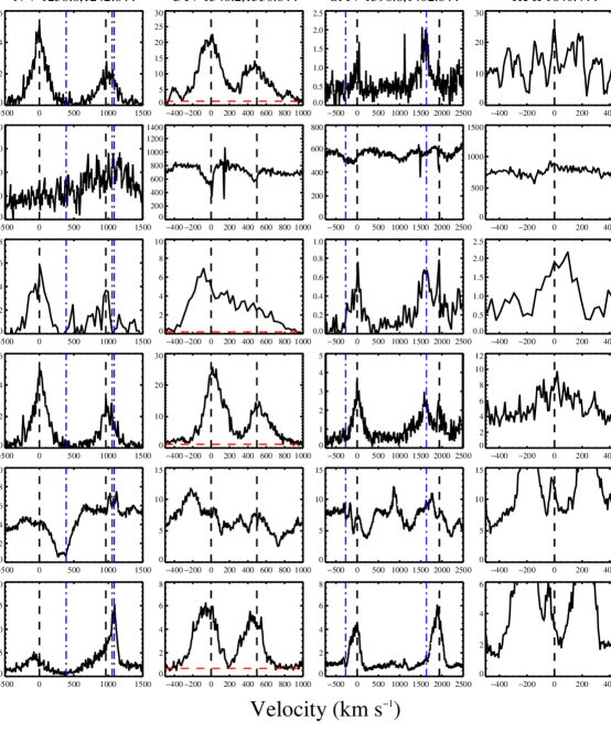
Figure 1.— Extracted line profiles for our sample. The rest wavelengths of the line is marked with a vertical dashed black line. Rest wavelengths of contaminating features are marked with vertical blue dot–dashed lines. The contaminating lines in the Si IV column are the CO A–X (5–0) band head at $-271$ km s^-1 and O IV $\lambda$1401 at $+1633$ km s^-1. In the N V column the contaminating lines are Mg II $\lambda$1240.4 at $+387$ km s^-1 and N I $\lambda$1243.2,1243.3 at $+1055$ and $+1085$ km s^-1. Continuum flux levels in the C IV panels are marked with a horizontal dashed red line.

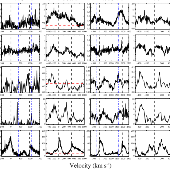
Figure 2.— Same as Figure 1 but for the remaining objects in the sample.

Table 1Log of HST STIS/COS observations

Object ID	Data ID	Instrument	Grating	Aperture	UT Date	Integration time (s)	Binning (pixels)	S/N @ 1550 Å
(1)	(2)	(3)	(4)	(5)	(6)	(7)	(8)	(9)
HD 139614	OC2H05020	STIS	E140M	0.2”x0.2”	2013–06–24	1670	3	6
	OC2H05030	STIS	E140M	0.2”x0.2”	2013–06–24	2758
HD 141569	OC2H04020	STIS	E140M	0.2”x0.2”	2013–07–19	1375	3	25
	OC2H04030	STIS	E140M	0.2”x0.2”	2013–07–19	2340
HD 142666	OC2H03020	STIS	E140M	0.2”x0.2”	2013–07–16	1624	10	5
	OC2H03030	STIS	E140M	0.2”x0.2”	2013–07–16	2763
HD 169142	OC2H02020	STIS	E140M	0.2”x0.2”	2013–07–11	1732	3	6
	OC2H02030	STIS	E140M	0.2”x0.2”	2013–07–11	2761
HK Ori	LC2H06010	COS	G160M	PSA	2012–12–06	1696	3	15
	LC2H06020	COS	G130M	PSA	2012–12–06	1856
KK Oph	LC2H08010	COS	G160M	PSA	2013–06–18	1556	3	7
	LC2H08020	COS	G130M	PSA	2013–06–18	1856
RR Tau	LC2H07010	COS	G160M	PSA	2012–12–07	1848	3	5
	LC2H07020	COS	G130M	PSA	2012–12–07	1856
T Ori	LC2H09010	COS	G160M	PSA	2012–12–06	1696	3	7
	LC2H09020	COS	G130M	PSA	2012–12–06	1856
VV Ser	LC2H10010	COS	G160M	PSA	2012–05–15	1696	10	4
	LC2H10020	COS	G130M	PSA	2013–05–15	1856
XY Per	OC2H01020	STIS	E140M	0.2”x0.2”	2012–10–12	1613	6	3
	OC2H01030	STIS	E140M	0.2”x0.2”	2012–10–12	2752

Table 2Stellar parameters

		$v_{rad}$	$M_{*}$	$R_{*}$	$v$sin$i$
Object ID	Spectral Type	(km s-1)	(${\rm\,\it{M_{\odot}}}$)	(${\rm\,\it{R_{\odot}}}$)	(km s-1)	Referencesa
(1)	(2)	(3)	(4)	(5)	(6)	(7)
HD 139614	A7	0.3	1.80	1.77	13	1,5,11
HD 141569	A0	35.7	2.33	1.94	228	1,2
HD 142666	A5	-7.0	2.15	2.82	65	1,3
HD 169142	A5	-0.4	1.69	1.64	48	1,5
HK Ori	A3	14.4	3.00	4.10	60	2,4,6
KK Oph	A8	10.0	2.17	2.94	$\cdots$	2,6,10
RR Tau	A0	15.3	5.80	9.30	225	2,6,7
T Ori	A3	56.1	3.13	4.47	147	1,2,8
VV Ser	B7	-2.0	4.00	3.10	124	1,7,8
XY Per	A2	2.0	1.95	1.65	224	1,3,8
DX Cha	A7	14.0	2.0	0.84	$\cdots$	5,9
41 Ari	B8	4.0	$\cdots$	$\cdots$	175	$\cdots$
$\alpha$ CMa	A0	-5.5	$\cdots$	$\cdots$	17	$\cdots$
HD 42111	A3	25.3	$\cdots$	$\cdots$	288	$\cdots$

3. LINE PROFILES

The extracted line profiles are shown in Figure 1 and Figure 2. The rest velocity of the lines is marked with a black dashed line. Nearby lines that potentially contaminate the lines of interest are marked with vertical dashed–dotted blue lines.

Unlike CTTSs, HAEBES have non-negligible photospheric flux at UV wavelengths. To aid in identifying the circumstellar features, we compare each object spectrum with a main sequence dwarf standard of similar spectral type. These standards are listed in the last four lines of Table 2. The standard spectra were obtained from StarCAT, a compilation of UV stellar spectra obtained with STIS (Ayres 2010). These comparisons are shown for C IV in Figure 3. Although we only show the kinematically important regions of the spectra in Figure 1 and Figure 2, approximately 10 Å of spectrum on either side of the lines are compared to a standard in order to approximately scale and match the standard to the object. For most objects, this allows unambiguous identification of photospheric features and allows a better estimate of the continuum to be made (horizontal red lines in Figure 1 and Figure 2; see Table 4).

We note that there is a lack of high-resolution UV observations of main sequence, late A-type dwarfs. Thus for the late A-type stars in our sample we use the A3 standard HD 42111. Due to the strong emission lines in these objects, the spectral type mismatch does not affect the analysis.

Figure 3.— Comparison of the observed C IV lines (black) with a spectroscopic main sequence standard of a similar spectral type (red). The standard is scaled to match the photospheric features of the object. The standards shown for HD 141569 and RR Tau were rotationally broadened. The rest velocities of the C IV doublet members are marked with vertical blue dashed lines.

Table 3Literature distance, extinction, and accretion rate values

	AV (mags)/Distance (pc)						log10($\dot{M}$) (${\rm\,\it{M_{\odot}}}$ yr-1)
Object ID	A13	F15	H04b	G06	V03		F15	M11	G06	DB11
(1)	(2)	(3)	(4)	(5)	(6)		(7)	(8)	(9)	(10)
HD 139614	0.50	0.00	$\cdots$	0.10	$\cdots$		-7.63	$\cdots$	-7.99	$\cdots$
	142	140	$\cdots$	150	$\cdots$
HD 142666	1.60	0.50	$\cdots$	0.80	1.15		$<$-8.38	-6.73	-8.00	-7.77
	145	145	$\cdots$	116	$\cdots$
HD 169142	-0.30	$\cdots$	$\cdots$	0.30	$\cdots$		$\cdots$	$\cdots$	-7.40	$\cdots$
	145	$\cdots$	$\cdots$	145	$\cdots$
KK Oph	$\cdots$	2.70	$\cdots$	0.44	0.90		$<$-7.84	-5.85	-7.91	$\cdots$
	$\cdots$	279	$\cdots$	160	$\cdots$
RR Tau	$\cdots$	$\cdots$	2.00/3.20	$\cdots$	4.52		$\cdots$	-4.11	-6.68	$\cdots$
	$\cdots$	$\cdots$	800	$\cdots$	$\cdots$
VV Ser	5.35	$\cdots$	3.40/5.40	3.10	$\cdots$		$\cdots$	$\cdots$	-6.34	-7.49
	260	$\cdots$	440	260	$\cdots$
DX Cha	$\cdots$	0.00	$\cdots$	0.70	0.44		-6.68	$\cdots$	-7.45	$\cdots$
	$\cdots$	115	$\cdots$	116	$\cdots$

Table 4C IV line parameters

	V${}^{blue}_{max}$	V${}^{red}_{max}$		$F_{cont}\times 10^{14}$	$F_{CIV}\times 10^{14}$a
Object ID	(km s-1)	(km s-1)	$F^{blue}_{max}/F^{red}_{max}$	(erg cm-2 s-1 Å-1)	(erg cm-2 s-1)	$L_{CIV}$/$L_{\odot}$b
(1)	(2)	(3)	(4)	(5)	(6)	(7)
HD 139614	-13.5	-23.2	1.71	1.23	52.7$\pm$0.9	3.3-11.0$\times$10-4
HD 142666	-105.1	-14.4	2.34	0.04	20.2$\pm$0.5	4.4-61.4$\times$10-4
HD 169142	28.7	-1.6	1.82	1.12	50.6$\pm$0.9	1.6-68.0$\times$10-4
KK Oph	-50.9	-55.1	1.17	0.55	14.9$\pm$0.1	1.0-234.8$\times$10-3
RR Tau	-191.2	-215.4	1.22	0.25	4.2$\pm$0.1	0.10-42.9
VV Ser	-265.1	-223.0	1.62	0.11	$>$0.4$\pm$0.07	1.4-356.0$\times$10-2
DX Cha	31.1	27.2	1.65	16.8	221.7$\pm$0.8c	9.2-49.8$\times$10-4

3.1. N V 1238.8,1242.8 Å

The N V doublet in our sample is in emission in 6 out of 11 objects. With the exception of DX Cha, none of the emission lines show any clear sign of absorption. The absorption in the blue wing of the red doublet member of the DX Cha profile is most likely due to a N I transition since it does not appear in the blue doublet member. The emission strength in HD 142666, RR Tau, and KK Oph seems to be comparable for both doublet members, although the true flux level of the red doublet member is obscured by N I emission in the RR Tau and KK Oph profiles.

3.2. C IV 1548.2,1550.8 Å

Six of the eleven objects show clear emission in the C IV doublet. Two objects, HD 142666 and RR Tau show broad emission such that the two distinct members of the doublet are not clearly identified. The apparent emission features of T Ori and XY Per are approximately consistent with a photospheric spectrum of similar spectral type. The profiles of VV Ser and HK Ori show deviations from the photospheric standard profiles, suggesting a circumstellar component. However, higher signal-to-noise observations and a more precise standard comparison are needed to verify the nature of the difference. Three objects, HD 139614, HD 169142, and DX Cha, show visual evidence of asymmetric profile shapes and differing morphologies between doublet members. HD 141569 is the only object that shows sharp blue–shifted absorption features. The absorption extends to $\sim$-150 km s^-1, suggestive of a relatively weak outflow.

3.2.1 The C IV line luminosity and mass accretion rate

Johns–Krull et al. (2000) were the first to demonstrate a relationship between accretion rate and C IV line luminosity for CTTSs. They interpreted the excess C IV flux, the flux remaining after magnetic surface activity is taken into account, as being produced in the accretion flow onto the star. Yang et al. (2012), for a sample of 37 CTTSs, confirmed the relationship between accretion luminosity ($L_{acc}$) and C IV line luminosity. They also showed that CTTSs show greater C IV line luminosities as a group than WTTSs, strengthening the conclusion that the C IV line flux is produced by mass accretion. This relationship was further confirmed by A13 for a sample of 28 CTTSs, although they point out that, due to the complexity of the physical processes producing the C IV flux, along with the intrinsic variability of CTTSs, the exact relationship between $\dot{M}$ and $L_{CIV}$ is uncertain. This relationship has not been extended to the higher mass HAEBES, although a weak correlation was found between $L_{acc}$ and $L_{CIV}$ for the intermediate mass TTSs by Calvet et al. (2004).

We have measured the C IV line fluxes for the HAEBES in our sample that show clear emission lines. This criteria excludes HD 141569, T Ori, and XY Per from the analysis. We also exclude HK Ori since most of the flux in the red-ward doublet member is absent or possibly absorbed by the blue-ward doublet member. We include VV Ser since the emission in the red-ward doublet member is still prominent.

Estimates of $L_{CIV}$ are very sensitive to $A_{V}$. Thus the chosen $A_{V}$ value dominates any random errors, e.g., the measured flux uncertainties or the formal uncertainties derived for $A_{V}$ or the object distance. $A_{V}$ is also affected by intrinsic accretion and brightness variations of the system, as well as the choice of total to selective extinction, $R_{V}$. For most of the objects in our sample, there is a wide range of $A_{V}$ and $\dot{M}$ reported in the literature. Values of $A_{V}$ can differ based on how they are determined, whether using photometric colors (e.g., Hernández et al. 2004; Alecian et al. 2013; Fairlamb et al. 2015) or spectroscopic template fits (e.g., Valenti et al. 2003). We have collected these values, as well as distances, from the recent studies of Alecian et al. (2013), Fairlamb et al. (2015), Hernández et al. (2004), Garcia Lopez et al. (2006), Valenti et al. (2003), Mendigutía et al. (2011), and Donehew & Brittain (2011). They are given in Table 3. We do not give the formal uncertainties from these studies since, if they are provided, they are typically much smaller than the range of reported values. Instead, we calculate $L_{CIV}$ for the full range of $A_{V}$. There is generally better agreement in distance determinations and so we use the median distance value for each object.

We choose to use $R_{V}$=3.1 for the $L_{CIV}$ calculations. There has been some effort by various authors to determine the appropriate value of $R_{V}$ for calculating extinction values towards HAEBES. Calvet et al. (2004), for example, find that anomalous extinction laws that closely resemble the $R_{V}$=3.1 standard interstellar function are better suited for their sample of intermediate mass CTTSs. Hernández et al. (2004) find better agreement between $A_{V}$ derived from two different colors, $B-V$ and $V-R$, by using $R_{V}$=5.0. However, for $A_{V}$$<$2.0 there is little difference between the $R_{V}$=3.1 and $R_{V}$=5.0 cases. Furthermore, $R_{V}$=3.1 is adopted by a majority of the studies from which the $A_{V}$ values are taken; $R_{V}$=5.0 is used in Hernández et al. (2004) and Alecian et al. (2013). Choosing $R_{V}$ =3.1 thus provides the most consistency across studies. We note that using $R_{V}$=5.0 shifts $L_{CIV}$ to lower values (i.e., to the left in Figure 4) but maintains the trend found using $R_{V}$=3.1. Given the highly uncertain nature of $L_{CIV}$, regardless of the chosen value of $R_{V}$, the adopted $R_{V}$ does not affect the overall conclusions.

The doublet line flux was calculated by subtracting the continuum flux from Table 4 across the line and integrating the flux, centered on the 1548.2 Å doublet member, from -500 to 900 km s^-1. This velocity range was chosen to be consistent with Ardila et al. (2013). For VV Ser, only the emission components of the line profile are included in the integration. We take this to be a lower limit on the total emission. The integrated flux value is then corrected for extinction using the $A_{V}$ values in Table 3 and an extinction law with $R_{V}$=3.1. The line luminosity is then calculated using the median distance in Table 3. The final values of $F_{CIV}$ and the range of $L_{CIV}$ are given in Table 4. The accretion rates are not simultaneous with the C IV measurements.

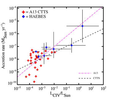
Figure 4.— C IV line luminosities versus accretion rate for the extinction–corrected CTTSs from A13 (red crosses) and the HAEBES from this study (blue diamonds). The best–fit relationship for the CTTS sample found by A13 is shown in pink. The best–fit relationship for the A13 CTTS sample using values of $A_{V}$ from Herczeg & Hillenbrand (2014) and Furlan et al. (2009, 2011). The $L_{CIV}$ error bars for the HAEBES represent the minimum and maximum values obtained using each of the literature $A_{V}$ values from Table 3. Error bars for $\dot{M}$ show the maximum and minimum literature values from Table 3.

Figure 4 shows $\dot{M}$ plotted against $L_{CIV}$ for the CTTS sample from A13 and the HAEBE sample from this study. For the HAEBES, the average value in log-space of $L_{CIV}$ is shown. The magenta line is the linear relationship found by A13 for their entire CTTS sample. The black dashed in Figure 4 is the relationship we find for the A13 CTTSs but using values of $A_{V}$ from Herczeg & Hillenbrand (2014) and Furlan et al. (2009, 2011). Herczeg & Hillenbrand (2014) derive values of $A_{V}$ by fitting a large grid of low-extinction spectral templates plus a flat accretion spectrum to their CTTS sample. Furlan et al. (2009, 2011) use photometric colors compared with photospheric template colors, and an assumption about the underlying excess accretion emission, to calculate $A_{V}$. The $A_{V}$ values from A13 come from a variety of sources but a significant fraction ($\sim$40%) are taken from Gullbring et al. (1998). The main difference in the derivation of $A_{V}$ across these studies is how the excess accretion and inner disk emission is treated, if it is considered in detail at all. How the excess emission is determined is likely a larger driver of the differences in $A_{V}$ than the difference between photometric and spectroscopic methods. The significantly different linear fits in Figure 4 demonstrate how the adopted value of $A_{V}$ can strongly affect the $L_{CIV}$-$\dot{M}$ relationship.

Although the number of objects is small, the HAEBES generally show an increase of $L_{CIV}$ with increasing $\dot{M}$, suggesting a common origin for the line flux in both types of objects. The large spread in $\dot{M}$ and $A_{V}$ for the HAEBES prevents any meaningful linear relationship from being extended into the HAEBE regime. In any case, as shown in Figure 4, this relationship is very uncertain for the CTTS sample. Observations of a larger sample of HAEBES, combined with simultaneous determinations of $\dot{M}$ and $A_{V}$, will be beneficial in further constraining the relationship between $\dot{M}$ and $L_{CIV}$ across a broad stellar mass range.

3.3. Si IV 1398.8,1402.8 Å

Six objects show clear emission signatures in Si IV. The Si IV line profiles can be contaminated by nearby CO A-X (5-0) bandhead emission (1393 Å, -271 km s^-1) and O IV emission (1401 Å, +1633 km s^-1). All objects displaying C IV emission, with the exception of VV Ser, show some sign of emission in Si IV. DX Cha is the only object in the sample that shows a clear blue–shifted absorption signature in Si IV: the emission profiles are sharply cut off at zero velocity, indicating a strong absorbing wind. DX Cha’s C IV line shows a similar morphology although the red and blue components differ more strongly.

3.4. He II 1640.5 Å

Compared to the CTTS sample of A13, He II emission is relatively uncommon in our sample: only 5 objects (HD 142666, HD 169142, HK Ori, KK Oph, and DX Cha) show clear signs of an emission profile. The strong emission lines to both sides of zero velocity in the line profiles of HK Ori, KK Oph, VV Ser, XY Per, and DX Cha are likely complexes of nearby Fe II lines. The relative absence of He II emission in our sample, and the presence of strong Fe II features, contrasts strongly with the ubiquitous He II emission lines, and lack of Fe II lines, seen in the CTTS sample from A13. This is consistent, however, with the general lack of He I 5876 Å emission seen in the optical HAEBE sample from Cauley & Johns–Krull (2015). The presence of strong Fe II features in the HAEBE UV spectra also reinforces the findings from Cauley & Johns–Krull (2015) that Fe I is largely absent from HAEBE spectra due to the intense ionizing flux emitted by HAEBE photospheres. The lack of He II emission in the HAEBE sample will be more fully explored in Section 5.

4. INVESTIGATING THE C IV MORPHOLOGIES

In young stars, C IV line flux can be formed in at least three distinct scenarios: the accretion flow onto the star, hot outflows (e.g., a stellar wind), or in the transition region/chromosphere. If the emitting region is optically thin, the resulting profile would be purely in emission; if the optical depth is large enough, the emission line will show signs of self absorption. However, it can be non-obvious distinguishing between asymmetric emission line profiles that form as a result of self absorption versus those that form as a result of having multiple emission components. The C IV doublet is especially useful for identifying potential outflows: the velocity separation of the doublet ($\sim$500 km s^-1 ) is small enough that optically thick outflows with terminal velocities near the velocity separation of the doublet should show evidence of absorption in the red wing of the blue doublet member.

In order to investigate the origin of the observed line profiles, we compare simple, pure scattering stellar wind model fits (i.e., emission profiles with absorption) with multi-Gaussian fits meant to represent emission lines formed in an accretion flow or chromosphere (i.e., pure emission lines with no absorption). Simple $\beta$–velocity wind laws, like the one that we employ here, have been shown to be good descriptions of the velocity structure in the winds of O–type stars (e.g. Lamers & Morton 1976; Groenewegen & Lamers 1989) and multi-Gaussian fits are good approximations of the pure emission line profiles in CTTSs, which are believed to form in the accretion flow onto the star (Ardila et al. 2013).

4.1. Multi–component Gaussian fitting

A13 found that the UV doublet emission line profiles of CTTSs can be accurately described by fitting two Gaussians or a single Gaussian to each doublet member. The objects requiring a two-Gaussian fit generally show evidence of a broad component and a narrow component. The broad component is believed to form along the accretion stream while the narrow component is formed in the post-shock gas at the stellar surface (Calvet & Gullbring 1998; Ardila et al. 2013). For CTTSs, A13 argue in favor of these hot gas lines being produced in the accretion flow onto the star. They cannot, however, rule out their formation in the stellar transition region, though the large velocity motions needed for the broad component argues against this interpretation. In this section we perform multi–component Gaussian fits to the C IV doublets in order to investigate the origin of the C IV line emission in HAEBES. Only objects which show pure emission features are included. This excludes HD 141569, T Ori, and XY Per, which closely match their photospheric templates, and HK Ori and VV Ser, which show evidence of a non-stellar contribution.

We fit each emission doublet with two different combinations of Gaussians: 1. a four–Gaussian fit composed of a broad and narrow component for each doublet member; 2. a single Gaussian for each doublet member, i.e., a two–Gaussian fit. The four–Gaussian fit has the following form:

$$\begin{split}F_{tot}=h_{1}\exp\Big{(}{-\frac{(v-v_{1})^{2}}{2\sigma_{1}^{2}}}\Big{)}+h_{2}\exp\Big{(}{-\frac{(v-v_{2})^{2}}{2\sigma_{2}^{2}}}\Big{)}+\\ h_{3}\exp\Big{(}{-\frac{(v-v_{1}-v_{off})^{2}}{2\sigma_{1}^{2}}}\Big{)}+\\ h_{4}\exp\Big{(}{-\frac{(v-v_{2}-v_{off})^{2}}{2\sigma_{2}^{2}}}\Big{)}+1\end{split}$$ (1)

where $h$ is the height of the Gaussian, $v$ is the velocity offset, $\sigma$ is the width of the Gaussian in km s^-1 , and $v_{off}$ is the velocity separation of the doublet (500.96 km s^-1 ). A continuum of 1.0 is added to the sum of the components. Thus the two broad components have the same velocity offset, $v_{1}$, and the same width, $\sigma_{1}$, and likewise for the narrow components. The two–Gaussian fit is simply Gaussians 1 and 3 from Equation 1. We fit for the parameters $h_{1}$, $v_{1}$, $\sigma_{1}$, $h_{2}$, $v_{2}$, $\sigma_{2}$, $h_{3}$, and $h_{4}$. The two–Gaussian fits involve fitting for $h_{1}$, $v_{1}$, $\sigma_{1}$, and $h_{3}$. We utilize a non–linear least–squares fitting routine based on the Marquardt method to determine the profile fits (see Bevington & Robinson 1992) and the normalized Poisson uncertainties are used to weight the individual points. The best–fit parameters for each object showing C IV emission are given in Table 5. The fits and the individual Gaussians are shown in Figure 5.

The C IV profiles of HD 139614, HD 169142, and KK Oph are all well described by both a two- and a four–Gaussian fit. The spectrum of HD 142666 has very low S/N and we suspect that the significant emission between the rest velocities of the C IV components is actually a separate N V emission component (see Section 3.1) and not the result of a narrow and broad C IV component. This is similar to the profile of RR Tau which also appears to be adequately described by a 4-Gaussian fit. Due to asymmetric appearance of the blue and red wings of HD 169142’s C IV doublet members, the profile will be investigated using the wind model in the next section.

Although the observed doublet components of DX Cha clearly do not have the same shape, we have shown the Gaussian fits to the DX Cha profile for illustration. The peak Gaussian fluxes for the broad components of the DX Cha fit (Table 5) have a blue–to–red component ratio of 0.30. In an optically thin or effectively thin gas, the blue–to–red component ratio of the C IV doublet emission lines is 2.0, as determined by the statistical weights of the atomic levels. As the medium becomes more optically thick and the lines thermalize, this ratio approaches 1.0. This is evidence that the observed DX Cha line profile is not simply the sum of various emission components and suggests that the wind interpretation, which will be explored quantitatively in the next section, is a more accurate description of the physical process producing the doublet morphology.

Table 5C IV Gaussian fit parameters

	$h_{1}^{a}$	$v_{1}$	$\sigma_{1}^{b}$	$h_{2}$	$v_{2}$	$\sigma_{2}$	$h_{3}$	$h_{4}$
Object	($F_{cont}$)	(km s-1)	(km s-1)	($F_{cont}$)	(km s-1)	(km s-1)	($F_{cont}$)	($F_{cont}$)	$\chi_{\nu}^{2}$
(1)	(2)	(3)	(4)	(5)	(6)	(7)	(8)	(9)	(10)
HD 139614	14.1	-17.7	100.4	1.8	7.0	279.2	6.9	1.9	0.73
HD 142666	44.3	-129.1	78.9	30.3	102.5	104.8	17.2	9.5	0.81
HD 169142	18.2	35.7	91.3	1.6	65.0	225.0	8.8	1.2	0.65
KK Oph	5.7	8.9	80.4	6.9	-117.6	99.0	5.1	4.9	7.52
RR Tau	1.57	69.0	71.4	3.53	-214.7	133.2	1.51	2.21	1.25
DX Cha	5.5	43.4	49.0	0.8	199.8	162.4	2.3	2.7	24.7
HD 139614	15.1	-13.6	100.4	$\cdots$	$\cdots$	$\cdots$	8.9	$\cdots$	0.83
HD 142666	44.4	-25.2	78.9	$\cdots$	$\cdots$	$\cdots$	18.1	$\cdots$	1.13
HD 169142	18.6	38.0	91.3	$\cdots$	$\cdots$	$\cdots$	10.0	$\cdots$	0.71
KK Oph	10.0	8.9	-56.4	$\cdots$	$\cdots$	$\cdots$	7.89	$\cdots$	8.06
RR Tau	3.17	-163.7	182.4	$\cdots$	$\cdots$	$\cdots$	2.11	$\cdots$	1.45
DX Cha	5.4	43.4	54.6	$\cdots$	$\cdots$	$\cdots$	4.6	$\cdots$	99.0

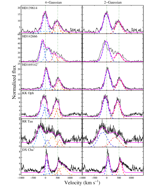
Figure 5.— Multi–component Gaussian fit to the C IV emission lines. The left-hand column shows the 4-Gaussian fit and the right-hand column shows the 2-Gaussian fit. The data is shown in black and the fit is shown in magenta. The individual Gaussians are shown in blue and light blue for the blue doublet member and red and orange for the red doublet member. The rest velocities of the doublet members are marked with vertical green lines. The objects marked with a + are the objects we fit using the stellar wind model. Note the large intensity of the broad component for the red doublet member of DX Cha (orange dashed line) compared to the broad component of the blue doublet member (light blue dashed line): this is unphysical due to the C IV 1548,1550 Å atomic parameters. For HD 139614, HD 169142, and KK Oph, the 2-Gaussian fit is comparable to the 4-Gaussian fit. HD 142666 and RR Tau are more accurately described by a 4-Gaussian fit (however, see Section 5.3).

4.2. Stellar wind model

Our pure-scattering model is parametrized and designed to demonstrate optical depth effects on the profile morphologies in closely spaced doublets (e.g., the UV C IV doublet). We do not derive physical parameters (e.g., temperature and mass loss rate) of the wind. We follow a treatment similar to Castor & Lamers (1979). Our model consists of a non–rotating, spherical star launching a spherically symmetric scattering wind, as suggested for young stars, for example, by Dupree et al. (2005). The outflowing material is assumed to originate at the stellar surface and is accelerated outward according to Equation 2:

$$v(r)=v_{o}+(v_{\infty}-v_{o})(1-\frac{R_{*}}{r})^{\beta}$$ (2)

where $v_{\infty}$ is the terminal wind velocity, $v_{o}$ is the initial wind velocity, $\beta$ is a positive non–zero number, and $r$ is the radial distance from the origin. Here, we assume the wind is essentially isothermal in that we assume a constant ionization fraction throughout the wind. Under this assumption the optical depth at each velocity $\tau$ becomes a function of only the density and $r$. The density at each $r$ can be assigned based on the mass continuity equation assuming a spherically symmetric outflow with a constant mass loss rate:

$$\rho(r)=\frac{\dot{M}}{4\pi r^{2}v(r)}$$ (3)

where $\dot{M}$ is the mass loss rate in the wind. For our purposes, the specific value of $\dot{M}$ is irrelevant since we only care about the fraction of the original material along the line of sight to the star at each $r$ and we parameterize the wind in terms of the total optical depth.

The integration along the line of sight through the wind is done through a series of equally spaced shells in velocity space. The initial and final velocities of a shell each define a unique radial distance from the star according to Equation 2. We also extend the range of absorbing velocities on either side of each shell to plus and minus half of the chosen velocity step. This acts as a natural line width, which we designate $\delta$$v$, since one is not explicitly included in the model. We define the optical depth at each absorbing velocity shell $v$ as

$$\tau(r_{v})=\frac{\rho_{r}\Delta r}{\sum\limits_{i}\rho_{i}\Delta r_{i}}$$ (4)

where $r_{v}$ is the center of the annulus at velocity $v$. Thus each annulus of physical width $\Delta$$r$ contains a fraction of the total optical depth, which is the optical depth at line center for the annulus at $r_{v}$, specified by Equation 4. For each annulus, the amount of absorbed intensity is then equal to $I_{r}$$e^{-\tau(r_{v})}$ where $I_{r}$ is the intensity incident upon the annulus. The absorbing velocities range from the maximum shell velocity down to $v_{f}$=$v_{r}$cos$\theta$-$\delta$$v$ where $\theta$=sin^-1($R_{*}$/$r$). Thus as the wind moves farther from the star the range of absorbing velocities becomes smaller. The geometry of the model is shown in Figure 6.

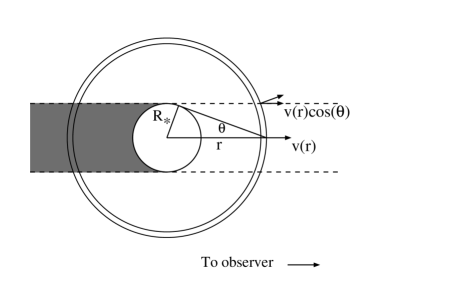
Figure 6.— Geometry of the stellar wind model. The shaded gray region illustrates the scattering region that does not contribute to the emission profile since these photons are absorbed by the star. The observer is to the right.

We also assume single, isotropic, and completely redistributive scattering (Lamers & Cassinelli 1999). Since the scattering is isotropic, the amount of scattered intensity in any annulus has to be equally redistributed in emission across velocities that range from -$v$($r$)-$\delta$$v$ to $v$($r$)$+\delta$$v$. Emission from velocities being blocked by the star (i.e., velocities of receding material immediately behind the star) is then set to zero since these photons hit the stellar surface and do not propagate back to the observer. The final line profile is the sum of the absorption profile and the emission profiles at each annulus.

Examples of the model for various input spectra are shown in Figure 7. Panel (a) shows a P-Cygni profile with a flat continuum as the input spectrum, similar to the profiles computed in the atlas by Castor & Lamers (1979). Panel (b) shows the effect of having a single Gaussian as the input spectrum, such as proposed by Dupree et al. (2005, 2014) for TW Hya. We note that the result is not a Gaussian but rather a P-Cygni profile. For significant absorption to be present in the blue wing while simultaneously preserving the Gaussian shape of the red wing of the input spectrum, few of the absorbed photons can be scattered back into the line of sight and the blue-wing continuum must be negligible so as not to reveal the sub-continuum absorption caused by the optically thick wind. If these conditions do not hold, the resulting line profile will not be Gaussian. Finally, panel (c) shows the resulting asymmetric line shapes of an optically thick wind in a doublet with a velocity separation identical to C IV: the red doublet member absorbs some of the flux that has been redistributed in the red wing of the blue doublet member.

The input spectrum for the fitting routine is a two–component Gaussian with a peak flux ratio of 2.0, which represents doublet emission from, for example, the base of an accretion flow or a chromosphere. Each component has the same full width at half maximum (FWHM) and they are centered at their respective wavelengths. Both the Gaussian FWHM and the ratio of the peak fluxes are allowed to vary in the fit. We also allow the total optical depth in the wind, $\tau$, to vary. The terminal velocity and velocity parameter $\beta$ are kept fixed at $v_{\infty}$=500 km s^-1 and $\beta$=1.0. We note that changing these fixed values to other reasonable numbers does not change the general results for most choices of $v_{\infty}$ and $\beta$. The same fitting routine mentioned in Section 4.1 is used for the stellar wind fits.

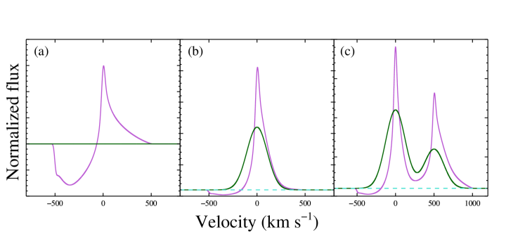
Figure 7.— Examples of the stellar wind model for different input spectra. The input spectrum is shown in green, the model output in purple, and in panels (b) and (c) the local continuum is shown in turquoise. Each model is calculated using the wind parameters $v_{term}$=500 km s^-1, $\tau$=200., and $\beta$=1.0. Panel (a) shows the case of a pure continuum input spectrum; panel (b) shows a single, strong Gaussian emission line as the input spectrum; panel (c) shows the case of a strong Gaussian emission doublet as the input spectrum. The resulting P–Cygni morphology of the panel (a) spectrum is obvious. In panel (c), the narrower width of the blue–ward doublet member can be seen, a result of the red–ward doublet member absorbing the flux in the red velocity wing of the blue–ward doublet member.

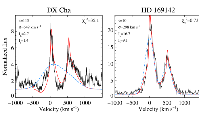
Figure 8.— Stellar wind model fits to the objects showing evidence of profile asymmetry. The observed normalized profile is shown in black; the best–fit input doublet profile is over plotted in blue; the best-fit wind model is shown in red. The total optical depth in the wind is shown in the upper–left corner of each panel, along with the best–fit input doublet emission line parameters: $I_{b}$ is the normalized peak intensity of blue doublet member, $I_{r}$ is the normalized peak intensity of the red doublet member, and $\sigma$ is the width of the input Gaussian. HD 169142 requires a marginal amount of outflowing material to explain the profile shape. DX Cha requires a large $\tau$ to reproduce the profile morphology, indicating the presence of a strong outflow. The emission bump at $\sim$-185 km s^-1 is H₂ emission and is ignored in the fit.

The results of the stellar wind model applied to DX Cha and HD 169142 are shown in Figure 8. It is immediately clear that the wind model favors a large optical depth for DX Cha and a moderate $\tau$ for HD 169142. Although the fitting program favors a small amount of optical depth for HD 169142, the differences between the best–fit model and the observed profile are well within the measured flux uncertainties. In addition, $\chi_{\nu}^{2}$ is worse for the wind than for either of the Gaussian fits. Thus we find little evidence for a hot wind in C IV for HD 169142 and favor the multiple emission components explored in Section 4.1.

DX Cha is the only object in the sample that clearly shows evidence of a strong outflow in the C IV doublet: the stellar wind model requires a total optical depth of $\tau$=113 to reproduce the shape of the profile. While the model does a fair job of reproducing the sharp cutoff at zero velocity and the narrow shape of the blue doublet component, the pure scattering treatment does a poor job of reproducing the red–shifted emission in the red component. This is not surprising as the model assumptions of spherical symmetry and a single emission component are likely incorrect. The stellar wind model clearly demonstrates the asymmetry of the red wing of the blue and red doublet components in the presence of a strong outflow. In addition, the multi-Gaussian fit to the DX Cha profile results in unphysical parameters for the emission lines, further suggesting that the profile morphology is the result of a hot outflow.

5. DISCUSSION

Although the sample of HAEBES presented here is small, the UV line profile morphologies and characteristics are diverse. Below we discuss some of the important features of the sample, how they relate to mass accretion and outflows, and how these characteristics compare to those of the CTTS sample from A13.

5.1. The general absence of hot optically thick outflows

The only object in our sample that shows clear evidence of an optically thick outflow in C IV is DX Cha. The C IV profile of HD 141569 shows signs of blue–shifted absorption but the absorption is very narrow and relatively weak. With the exceptions of DX Cha, HD 139614, and KK Oph, for which we do not have optical or He I 10830 Å data, our sample also shows no direct evidence of optically thick outflows in their optical or He I 10830 Å line profiles. Thus most of these objects not only show no evidence for hot outflows in the UV lines examined here, wind signatures are also absent from other wavelength regions of their spectra. The lack of observed outflows may be the result of HAEBES having relatively smaller magnetospheres compared to CTTSs. This possibility is discussed further in the next section. Regardless, it appears that hot, optically thick outflows are not common among our sample and, based on the relatively small percentage of objects showing optical (37%) or He I 10830 Å (40%) blue-shifted absorption (e.g., Cauley & Johns–Krull 2014, 2015), possibly among HAEBES in general. However, the lack of hot winds should be examined with a larger and more diverse sample of HAEBES.

The strong outflow seen in C IV for DX Cha (also known as HD 104237A) may be related to the presence of its short period T Tauri star companion (Feigelson et al. 2003; Böhm et al. 2004). It is likely part of a quintuple system with two or more T Tauri star companions orbiting DX Cha and its immediate companion (HD 104237B) at a distance of $\sim$1500 AU (Feigelson et al. 2003). Interactions between DX Cha and its close companion could drive the wind observed in C IV. This would explain why we observe a wind only for DX Cha since none of the other objects in our sample have confirmed companions with such close separations. Followup observations should be conducted to measure the C IV flux as function of orbital phase in order to investigate the effect of close companions on HAEBE C IV flux and profile morphology.

5.2. A relative paucity of C IV lines

We suggested in Cauley & Johns–Krull (2014, 2015) that HAEBES have smaller magnetospheres than CTTSs and that the relatively smaller disk truncation radii in HAEBES result in less of the necessary energy from the accretion flow being available to launch outflows from near the stellar surface. Although neither HAEBES nor CTTSs, in general, show evidence for strong outflows in the hot UV lines, the paucity of C IV and He II emission in our sample compared to the CTTS sample from A13 suggests that the smaller relative size of HAEBE magnetospheres and their apparent lack of strong magnetic fields may play a role in the lack of emission in the hot lines. We note that the free–fall velocities from, for example, $\sim$1.2 $R_{*}$ for the objects in our sample are similar to the free–fall velocities from 2.0–2.5 $R_{*}$ for a typical CTTS of mass 0.5 ${\rm\,\it{M_{\odot}}}$ and radius 1.5 ${\rm\,\it{R_{\odot}}}$. Then for a similar(larger) accretion rate, similar(greater) amounts of kinetic energy should be dissipated in the accretion shock. This would suggest that if hot outflows are a product of energy dissipation from the accretion flow that the hot gas lines in emission should be present in the spectra of accreting HAEBES. Thus the fact that the UV lines are observed in emission in only $\sim$50% ($\sim$60% if the profiles of VV Ser and HK Ori are included) of our sample, when all of our objects have measured accretion rates, suggests that the lack of strong emission in the hot UV lines is not a result of these objects not accreting material from their disks. Furthermore, both XY Per and T Ori, which show no evidence of C IV emission, show clear inverse P-Cygni profiles in their optical spectra.

One possible explanation for the relative lack of C IV and He II emission in our sample is that the temperature of the accretion shock in HAEBES is too low to produce these species. Temperatures below $\sim$10⁵ K may be insufficient to produce enough observable C IV flux. If we consider the strong shock regime, i.e., high Mach number, we can estimate the shock temperature using equation (9) from Calvet & Gullbring (1998). For typical HAEBE parameters of $M_{*}$=2.0 $M_{\sun}$ and $R_{*}$=2.0 $R_{\sun}$, shock temperatures are limited to 10⁵ K if material accretes from $r$$<$1.2 $R_{*}$. A typical infall radius inferred from the red-shifted absorption velocities in Cauley & Johns–Krull (2015) is $R_{in}$$\sim$1.1 $R_{*}$. This is significantly smaller than that for the CTTS sample from Fischer et al. (2008), which we calculate to be $R_{in}$$\sim$2.7 $R_{*}$. In reality, in-falling material likely originates from farther out in the disk. Projection effects may result in observed maximum red-shifted velocities that are smaller than the true maximum infall velocity of the material (Fischer et al. 2008). In general, however, the smaller values of $V_{red}$/$V_{esc}$ measured in Cauley & Johns–Krull (2014, 2015) are compatible with the idea that the infalling material for HAEBES may not be able to heat the post-shock material to temperatures capable of producing C IV emission.

For the stellar parameters typical of our sample and using $R_{in}$=1.1 $R_{*}$, the shock temperature is only $\sim$3.5$\times$10⁴ K compared to $\sim$8.5$\times$10⁵ K for the CTTS sample. Using the stellar parameters from Table 2, we calculate a typical corotation radius of $R_{co}$$\sim$1.6 $R_{*}$ for the rapid rotators ($v$sin$i$$>$100 km s^-1) in our sample. This is roughly consistent with the the fact that material accreting along magnetic field lines must originate at distances less than the corotation radius (e.g., Shu et al. 1994). However, if the true infall velocities are higher than the observed red-shifted velocities by only $\sim$20%, then the infall distance condition ($<$1.2 $R_{*}$) required for shock temperatures below 10⁵ K is no longer met for any of the HAEBES from Cauley & Johns–Krull (2015) with red-shifted absorption profiles. The effect of observing the accretion stream projected against the star could easily produce a difference of this magnitude. While it is plausible that the shock temperature of infalling material onto HAEBES could be lower than that for CTTSs, it is unclear exactly how large this difference is and if it is enough to explain the relative lack of C IV and He II emission seen here. Although this idea deserves further investigation, we tentatively suggest that the evidence of smaller magnetospheres in HAEBES is further supported by the C IV analysis presented here and, as a result of the lower shock temperatures produced by the infalling gas, C IV production is stunted compared to CTTSs.

5.3. The origin of the C IV emission lines

Ardila et al. (2013) established that most of the C IV emission observed from CTTSs requires a 4-component Gaussian to describe the line shape (a broad and narrow component for each doublet member) and is consistent with formation in an accretion flow, although a contribution from the stellar transition region cannot be ruled out. As we showed in Section 4.1, the C IV emission lines of HD 139614, HD 169142, and KK Oph are well described by a two component Gaussian. Of the pure emission profiles, HD 142666 is the only one that requires a 4-Gaussian fit. However, as we discussed in Section 3.2, the extra emission between the C IV doublet members may be due to N V. In any case, one commonality among the C IV emission line profiles of HD 139614, HD 142666, KK Oph, and RR Tau is that the peak flux is blue-shifted. HD 169142 shows a positive velocity for the peak flux in the blue doublet member.

In general, the blue-shifted velocities measured for the majority of the emission lines, and the hint of wind absorption in HD 169142, suggests that the C IV lines are being produced in optically thin outflowing material. If the C IV lines in our sample are the result of wind emission and a single emission component is required to fit the line morphology, this suggests that any mass accretion onto these objects is not directly responsible for the emission since emission produced by in falling material would result in red-shifted emission or emission centered close to zero velocity. Although this may seem to contradict the findings from Section 3.2.1, we are not inferring that mass accretion is not powering the UV lines but rather that the lines do not form directly in the accretion flows, e.g., along an in-falling accretion stream. Some of the accretion energy could be used to heat the atmosphere of the star and power the outflows, i.e., an accretion driven wind (Matt & Pudritz 2005). As the Gaussian fitting demonstrated, the C IV lines also seem to be pure emission profiles. In other words, they do not seem to be subject to any significant amount of absorption in the flow. Thus we suggest that the C IV emission line profiles in our sample are formed in weak, optically thin outflows, perhaps in an expanding stellar chromosphere or corona as first proposed by Catala et al. (1984) and Catala (1988) for AB Aur, that are likely accretion powered to some degree. This should be further tested with a larger sample of high signal-to-noise C IV HAEBE line profiles.

6. SUMMARY AND CONCLUSIONS

We have presented new high resolution UV spectra for a small sample of HAEBES and analyzed the line morphologies of the C IV 1548,1550 Å doublet for evidence of hot ($\sim$10⁵ K) winds. Although a larger sample of HAEBES should be examined to better understand these lines and their formation in HAEBES as a whole, we tentatively conclude the following:

• The $L_{CIV}$ vs. $\dot{M}$ relationship seems to extend to the HAEBE mass regime, suggesting a common origin for both CTTSs and HAEBES. A larger sample size of HAEBES is needed to confirm this. Differing values of $A_{V}$ can have a drastic effect on the $L_{CIV}$-$\dot{M}$ relationship and simultaneous measurements of $L_{CIV}$ and $\dot{M}$ are desirable.

• With the exception of RR Tau and HD 142666, the C IV emission lines in our sample are well described by a single Gaussian component. This contrasts with the C IV lines seen in CTTSs which require both a broad and narrow component for each doublet member. This fact, combined with the blue-shifted velocities observed for the peak fluxes of the pure emission lines, suggests that these line profiles in our sample are formed in weak outflows near the stellar surface and not in accretion flows onto the star. These outflows are likely accretion powered since all of these objects show signs of accretion in the optical.

• Only one object in our sample, DX Cha, shows strong evidence of an optically thick outflow in C IV. This is demonstrated with a simple wind scattering model. The existence of a strong wind may be due to the presence of a low mass companion with an orbital period of $\sim$20 days (Böhm et al. 2004). Although blue–shifted absorption has been observed in C IV in a few HAEBES (e.g., Grady et al. 1996), hot, optically thick outflows seem to be uncommon for HAEBES that also do not show evidence of outflows in the optical or at He I 10830 Å. Due to the relatively smaller percentage of HAEBES with blue-shifted absorption in their optical and He I 10830 Å lines, the lack of hot outflows observed here suggests they are also relatively uncommon for HAEBES in general. However, the statistics on the occurrence rate of winds in C IV are currently poor. An effort should be made to increase the number of objects with measured C IV profiles so that the morphologies and line characteristics can be adequately studied in a manner similar to A13.

Acknowledgments: We are grateful to the referee for their comments which helped improve the quality of the paper. We acknowledge funding from grant HST-GO-12996.001 from STSci and from grant NNX13AF09G through the NASA ADAP program. This research has made use of the SIMBAD database operated at CDS, Strabourg (France) and NASA’s Astrophysics Data System.

References

- Alecian et al. (2013) Alecian, E., et al. 2013, MNRAS, 429, 1001
- Ardila et al. (2013) Ardila, D. R., Herczeg, G. J., & Gregory, S. G., et al. 2013, ApJSS, 207, 1 (A13)
- Ayres (2010) Ayres, T. 2010, ApJS, 187, 149
- Bevington & Robinson (1992) Bevington, P. R., & Robinson, D. K. 1992, Data Reduction and Error Analysis for the Physical Sciences (2nd ed.; New York: McGraw-Hill)
- Böhm et al. (2004) Böhm, T., Catala, C., Balona, L., & Carter, B. 2004, A&A, 427, 907
- Bouret et al. (1997) Bouret, J.-C., Catala, C., & Simon, T. 1997, A&A, 328, 606
- Bouret & Catala (1998) Bouret, J.–C., & Catala, C. 1998, A&A, 340, 163
- Calvet & Gullbring (1998) Calvet, N., & Gullbring, E. 1998, ApJ, 509, 802
- Calvet et al. (2004) Calvet, N., Muzerolle, J., Briceño, C., et al. 2004, AJ, 128, 1294
- Cantiello & Braithwaite (2011) Cantiello, M., & Braithwaite, J. 2011, A&A, 534, A140
- Castor & Lamers (1979) Castor, J. I., & Lamers, H. J. G. L. M. 1979, ApJSS, 39, 481
- Catala et al. (1984) Catala, C., Kunasz, P. B., & Praderie, F. 1984, A&A, 134, 402
- Catala (1988) Catala, C. 1988, A&A, 193, 222
- Cauley & Johns–Krull (2014) Cauley, P. W., & Johns-Krull, C. M. 2014, ApJ, 797, 112
- Cauley & Johns–Krull (2015) Cauley, P. W., & Johns-Krull, C. M. 2015, ApJ, 810, 5
- Donehew & Brittain (2011) Donehew, B., & Brittain, S. 2011, AJ, 141, 46
- Drake et al. (2014) Drake, J. J., Braithwaite, J., Kashyap, V., Güenther, H. M., & Wright, N. J. 2014, ApJ, 786, 136
- Dupree et al. (2005) Dupree, A. K., Brickhouse, N. S., Smith, G. H., & Strader, J. 2005, ApJ, 625, L131
- Dupree et al. (2014) Dupree, A. K., Brickhouse, N. S., Cranmer, S. R., et al. 2014, ApJ, 789, 27
- Edwards et al. (2006) Edwards, S., Fischer, W., Hillenbrand, L., & Kwan, J. 2006, ApJ, 646, 319
- Edwards et al. (2013) Edwards, S., Kwan, J., Fischer, W., et al. 2013, ApJ, 778, 148
- Fairlamb et al. (2015) Fairlamb, J. R., Oudmaijer, R. D., Mendigutía, I., Ilee, J. D., & van den Ancker, M. E. 2015, MNRAS, 453, 976
- Feigelson et al. (2003) Feigelson, E. D., Lawson, W. A., & Garmire, G. P. 2003, ApJ, 599, 1207
- Finkenzeller & Jankovics (1984) Finkenzeller, U., & Jankovics, I. 1984, A&ASS, 57, 285
- Fischer et al. (2008) Fischer, W., Kwan, J., Edwards, S., & Hillenbrand, L. 2008, ApJ, 687, 1117
- Furlan et al. (2009) Furlan, E., Watson, D. M., McClure, M. K., et al. 2009, 703, 1964
- Furlan et al. (2011) Furlan, E., Luhman, K. L., Espaillat, C., et al. 2011, ApJSS, 195, 3
- Garcia Lopez et al. (2006) Garcia Lopez, R., Natta, A., Testi, L., & Habart, E. 2006, A&A, 459,837
- Grady et al. (1996) Grady, C. A., Pérez, M. R., Talavera, A., et al. 1996, A&ASS, 120, 157
- Grady et al. (2004) Grady, C. A., Woodgate, B., Torres, C. A. O., et al. 2004, ApJ, 608, 809
- Groenewegen & Lamers (1989) Groenewegen, M. A. T., & Lamers, H. J. G. L. M. A&AS, 79, 359
- Güenther & Schmitt (2009) Güenther, H. M., & Schmitt, J. H. M. M. 2009, A&A, 494, 1041
- Gullbring et al. (1998) Gullbring, E., Hartmann, L., Briceno, C., & Calvet, N. 1998, ApJ, 492, 323
- Hartigan et al. (1995) Hartigan, P., Edwards, S., & Ghandour, L. ApJ, 452, 736
- Herczeg & Hillenbrand (2014) Herczeg, G. J., & Hillenbrand, L. A. 2014, ApJ, 786, 97
- Hernández et al. (2004) Hernández, J., Calvet, N., Briceño, C., Hartmann, L., & Berlind, P. 2004, AJ, 127, 1682
- Hillenbrand et al. (1992) Hillenbrand, L. A., Strom, S. E., Vrba, F. J., & Keene, J. 1992, ApJ, 397, 613
- Ingleby et al. (2013) Ingleby, L., Calvet, N., & Herczeg, G., et al. 2013, ApJ, 767, 112
- Johns–Krull et al. (2000) Johns-Krull, C. M., Valenti, J. A., & Linsky, J. L. 2000, ApJ, 539, 815
- Johns–Krull & Herczeg (2007) Johns–Krull, C. M., & Herczeg, G. J. 2007, ApJ, 655, 345
- Kurosawa et al. (2011) Kurosawa, R., Romanova, M. M., & Harries, T. J. 2011, MNRAS, 416, 2623
- Kwan & Fischer (2011) Kwan, J., & Fischer, W. 2011, MNRAS, 411, 2383
- Lagrange et al. (1987) Lagrange, A. M., Ferlet, R., & Vidal-Madjar, A. 1987, A&A, 173, 289
- Lamers & Morton (1976) Lamers, H. J. G. L. M., & Morton, D. C. 1976, ApJSS, 32, 715
- Lamers & Cassinelli (1999) Lamers, H. J. G. L. M., & Cassinelli, J. P. 1999, Introduction to Stellar Winds (1st ed.; Cambridge: Cambridge University Press)
- Manoj et al. (2006) Manoj, P., Bhatt, H. C., Maheswar, G., & Muneer, S. 2006, ApJ, 653, 657
- Matt & Pudritz (2005) Matt, S., & Pudritz, R. E. 2005, ApJ, 632, L135
- Meeus et al. (1998) Meeus, G., Waelkens, C., & Malfait, K. 1998, A&A, 329, 131
- Mendigutía et al. (2011) Mendigutía, I., et al. 2011, A&A, 535, A99
- Mendigutía et al. (2012) Mendigutía, I., et al. 2012, A&A, 543, A59
- Mora et al. (2004) Mora, A., Eiroa, C., Natta, A., et al. 2004, A&A, 419, 225
- Mottram et al. (2007) Mottram, J. C., Vink, J. S., Oudmaijer, R. D., & Patel, M. 2007, MNRAS, 377, 1363
- Muzerolle et al. (1998) Muzerolle, J., Calvet, N., & Hartmann, L. 1998, ApJ, 492, 743
- Muzerolle et al. (2001) Muzerolle, J., Calvet, N., & Hartmann, L. 2001, ApJ, 550, 944
- Muzerolle et al. (2004) Muzerolle, J., D’Alessio, P., Calvet, N., & Hartmann, L. 2004, ApJ, 617
- Praderie et al. (1982) Praderie, F., Talavera, A., Felenbok, P., Czarny, J., & Boesgaard, M. 1982, ApJ, 254, 658
- Romanova et al. (2009) Romanova, M. M., Ustyugova, G. V., Koldoba, A. V., & Lovelace, R. V. E. 2009, MNRAS, 399, 1802
- Shu et al. (1988) Shu, F. H., Lizano, S., Ruden, S. P., & Najita, J. 1988, ApJ, 328, L19
- Shu et al. (1994) Shu, F., Najita, J., Ostriker, E., et al. 1994, ApJ, 429, 781
- Stelzer et al. (2006) Stelzer, B., Micela, G., Hamaguchi, K., & Schmitt, J. H. M. M. 2006, A&A, 457, 223
- Stelzer et al. (2009) Stelzer, B., Robrade, J., Schmitt, J. H. M. M., & Bouvier, J. 2009, A&A, 493, 1109
- Tout & Pringle (1995) Tout, C. A., & Pringle, J. E. 1995, MNRAS, 272, 528
- Valenti et al. (2003) Valenti, J. A., Fallon, A. A., & Johns-Krull, C. M. 2003, ApJSS, 147, 305
- Yang et al. (2012) Yang, H., Herczeg, G. J., Linsky, J. L., et al. 2012, ApJ, 744, 121
- Zanni & Ferreira (2013) Zanni, C., & Ferreira, J. 2013, A&A, 550, A99
- Zinnecker & Preibisch (1994) Zinnecker, H., & Preibisch, Th. 1994, A&A, 292, 152