Reduced dynamical maps in the presence of initial correlations

Abstract

We introduce a general framework for the construction of completely positive dynamical evolutions in the presence of system-environment initial correlations. The construction relies upon commutativity of the compatibility domain obtained by considering the marginals with respect to the environmental degrees of freedom of the considered class of correlated states. Our approach allows to consider states whose discord is not necessarily zero and explicitly show the non-uniqueness of the completely positive extensions of the obtained dynamical map outside the compatibility domain. The relevance of such maps for the treatment of open quantum system dynamics is discussed and connection to previous literature is critically assessed.

I Introduction

A ubiquitous situation in quantum physics involves the description of systems which are not isolated, so that their dynamics is actually influenced by other quantum degrees of freedom. The theory of open quantum systems was indeed developed to cope with such situations and has found important applications in diverse fields starting from quantum optics to condensed matter theory, chemical physics and many others Breuer2002 (1, 2). The standard description of an open quantum system dynamics rests on two basic assumptions, namely an initial system-environment state in factorized form and weak coupling between system and environment. In such a case the existence of a reduced dynamics is granted and it can reasonably be taken to obey a semigroup composition law in time, so that the most famous result by Gorini, Kossakowski, Sudarshan and Lindblad applies, fully characterizing the generator of such a dynamical semigroup Gorini1976a (3, 4). A lot of effort has been devoted to overcome these limitations within the standard framework in which the reduced open quantum system dynamics is obtained by tracing over the environmental degrees of freedom, but also different approaches have been recently proposed Bondar2014a (5).

Major results have been obtained in describing dynamics beyond the weak coupling limit, leading to reduced dynamical evolutions which go beyond a simple semigroup composition law. These strong coupling dynamics often show up memory effects. Indeed also in this respect important results have been obtained in providing a characterization of non-Markovian dynamics within open quantum system theory, and all of these results rely on the existence of a reduced system dynamics Rivas2014a (6, 7). On the contrary, despite important efforts Rodriguez2008a (8, 9, 10, 11, 12, 13, 14), the extension of the formalism to go beyond initially factorized states appears to be much harder, and a general satisfactory treatment still lags behind. Indeed such an extension is called for, since the choice of factorized initial states is well compatible with a weak coupling approach, but is generally not a natural assumption if one considers situations in which the coupling between system and environment degrees of freedom is actually strong.

Different paths have been followed in order to tackle the issue of initially correlated states between system and environment Grabert1988a (15, 16, 17, 18, 19), and in particular great attention has been devoted to study the conditions under which a completely positive map can be introduced to describe the reduced dynamics in the presence of initial correlations Pechukas1994a (20, 21, 9, 22, 10, 23).

In the usual framework of open quantum systems Breuer2002 (1) one considers a tensor product structure $\mathcal{H}_{S}\otimes\mathcal{H}_{E}$, where $\mathcal{H}_{S}$ and $\mathcal{H}_{E}$ denote the Hilbert space of system and environment respectively, and assumes that the overall system is closed, so that its time evolution can be described by a group of unitary operators $U_{SE}(t)$. Within this description, given an arbitrary initial system-environment state $\rho_{SE}(0)$, with corresponding reduced system state $\rho_{S}(0)=\operatorname{Tr}_{E}\rho_{SE}(0)$, where $\operatorname{Tr}_{E}$ denotes the partial trace with respect to the environment degrees of freedom, one can naturally consider the following collection of time dependent transformations

$$\rho_{S}(0) \rightarrow \rho_{S}(t)=\operatorname{Tr}_{E}[U_{SE}(t)\rho_{SE}(0)U_{SE}(t)^{{\dagger}}],$$ (1)

which by construction preserve positivity and trace. If the initial state $\rho_{SE}(0)$ is actually factorized, so that $\rho_{SE}(0)=\rho_{S}(0)\otimes\rho_{E}(0)$, it is well known that in such a way one obtains a linear map defined on the whole set of states, which in particular can be shown to be not only positive, but actually completely positive. The notion of complete positivity Nielsen2000 (24, 25) naturally emerges in this open quantum system setting and is indeed a typical quantum feature, related to the tensor product structure of the space describing a composite system. At the level of states one can witness the difference between positivity and complete positivity of a map by the application to entangled states, while at the level of observables the same difference can be appreciated by applying the map to non commuting set of observables. Indeed it is an important result that for a map acting on a commutative space positivity is equivalent to complete positivity Stinespring1955a (26, 27). More precisely the notions of positivity and complete positivity coincide if either starting or arrival space of the map is given by a commutative algebra, which therefore is amenable to a classical description Strocchi2005 (28).

In this article we will build on these basic facts to point out a general construction of completely positive maps arising in the presence of a correlated system environment state. As we shall see this approach allows us to recover as special cases some results previously obtained in the literature Rodriguez2008a (8, 11).

II Quantum maps and correlated states

II.1 General construction of quantum maps starting from correlated states

In order to consider the possibility to introduce completely positive maps starting from correlated system environment states let us first consider the following class of correlated states

$$\mathcal{C}_{SE} = \left\{\rho_{SE}=\sum_{i}p_{i}\sigma^{i}_{S}\otimes\rho^{i}_{E}\quad s.t.\quad[\sigma^{i}_{S},\sigma^{j}_{S}]=0\right\},$$ (2)

where $\{p_{i}\}_{i}$ is a probability distribution, the $\{\rho^{i}_{E}\}_{i}$ a collection of states for the environment, $\{\sigma^{i}_{S}\}_{i}$ a fixed set of commuting statistical operators for the system and we assume the Hilbert space of the system $\mathcal{H}_{S}$ to be finite dimensional with dimension $n$. The set $\mathcal{C}_{SE}$ provides a convex subset of the whole set of states on $\mathcal{H}_{S}\otimes\mathcal{H}_{E}$, which we denote by $\mathcal{S}(\mathcal{H}_{S}\otimes\mathcal{H}_{E})$. In particular it is a subset of the set of separable states which includes only zero discord states Ollivier2001a (29, 30). To this set we can associate a compatibility domain given by the set of system states which can be obtained as marginals of these correlated states, namely

$$\mathcal{C}_{S} = \left\{\rho_{S}=\sum_{i}p_{i}\sigma^{i}_{S}\right\},$$ (3)

which is still a convex set and is in particular a commutative set. Note however that the relationship between sets of correlated states and their compatibility domain is many to one, so that the same compatibility domain may arise from different classes of separable correlated states. The set  $\{\sigma^{i}_{S}\}_{i}$ is generated by a set of $d\leqslant n$ statistical operators with orthogonal support, where $d$ is the dimension of the linear hull of $\mathcal{C}_{S}$. If $d=n$ in particular $\mathcal{C}_{S}$ is given by the convex combinations of states which are all extremal. Supposing $d<n$, so that at least one of the $\{\sigma^{i}_{S}\}_{i}$, say $W$, is not necessarily a projection operator, without loss of generality we have

$$\{\sigma^{i}_{S}\}_{i} = \{\Pi_{\varphi_{1}},\ldots,\Pi_{\varphi_{d-1}},W\},$$ (4)

where $\{\varphi_{i}\}_{i=1,\ldots,d-1}$ are orthonormal vectors in $\mathcal{H}_{S}$ and we have introduced the one dimensional projections $\Pi_{\varphi_{i}}=|\varphi_{i}\rangle\langle\varphi_{i}|$. The statistical operator $W$, which is not a pure state, admits many different decompositions. In particular one can consider an orthogonal decomposition

$$W = \sum_{i=d}^{n}w_{i}|\varphi_{i}\rangle\langle\varphi_{i}|,$$ (5)

given by its spectral resolution, where the $\{\varphi_{i}\}_{i=d,\ldots n}$ are orthonormal vectors, further orthogonal to the span of $\{\varphi_{i}\}_{i=1,\ldots,d-1}$, so that altogether they provide a basis in $\mathcal{H}_{S}$, and the positive weights $w_{i}$ sum up to one. At the same time one can consider many others non orthogonal convex decompositions of the form

$$W = \sum_{k=1}^{r}\mu_{k}|\psi_{k}\rangle\langle\psi_{k}|,$$ (6)

with $r>n-(d-1)$ and where the $\{\psi_{k}\}_{k=1,\ldots,r}$ are normalized but generally non orthogonal states while $\{\mu_{k}\}_{k=1,\ldots,r}$ is a probability distribution. For a choice of system states of the form Eq. (4) the compatibility domain Eq. (3) can therefore be seen to arise from the two following distinct sets of correlated system environment states, namely

$$\mathcal{C}_{SE}^{I} = \left\{\rho_{SE}=\sum_{i=1}^{d-1}p_{i}|\varphi_{i}\rangle\langle\varphi_{i}|\otimes\rho^{i}_{E}+p_{d}\sum^{n}_{i=d}w_{i}|\varphi_{i}\rangle\langle\varphi_{i}|\otimes\varrho^{i}_{E}\right\}$$ (7)

and

$$\mathcal{C}^{II}_{SE} = \left\{\rho_{SE}=\sum_{i=1}^{d-1}p_{i}|\varphi_{i}\rangle\langle\varphi_{i}|\otimes\rho^{i}_{E}+p_{d}\sum_{k=1}^{r}\mu_{k}|\psi_{k}\rangle\langle\psi_{k}|\otimes\varrho^{k}_{E}\right\},$$ (8)

with $\sum_{i=1}^{d}p_{i}=1$, while $\{\rho_{E}^{i}\}_{i}$ and $\{\varrho_{E}^{k}\}_{k}$ are collections of distinct environmental states. While these composite states have the same compatibility domain according to Eq. (4), we have the important difference that while $\mathcal{C}_{SE}^{I}$ only contains zero quantum discord states, this is no more true for $\mathcal{C}^{II}_{SE}$, which thus also includes quantum correlations. Given an arbitrary system environment interaction $U_{SE}(t)$ we can now consider the transformation $\Phi^{II}(t)$ which associates to the marginal of a state $\rho_{SE}\in\mathcal{C}_{SE}^{II}$, that is

$$\rho_{S}(0) = \operatorname{Tr}_{E}\rho_{SE}$$ (9)

$$= \sum_{i=1}^{d-1}p_{i}|\varphi_{i}\rangle\langle\varphi_{i}|+p_{d}W,$$

the marginal associated to the time evolved state according to

$$\rho_{S}(0) \rightarrow \rho_{S}(t)=\operatorname{Tr}_{E}(U_{SE}(t)\rho_{SE}U^{{\dagger}}_{SE}(t)),$$ (10)

so that we set

$$\rho_{S}(t) = \Phi^{II}(t)[\rho_{S}(0)],$$ (11)

and an analogue construction can be done starting from states in $\mathcal{C}_{SE}^{I}$, thus obtaining a collection of maps $\Phi^{I}(t)$. We have now the important fact that such assignments actually define positive affine maps on the convex set $\mathcal{C}_{S}$, which can be uniquely extended to linear maps on the linear hull of $\mathcal{C}_{S}$. Since the elements of the set $\mathcal{C}_{S}$ commute, according to Stinespring1955a (26, 27) we therefore have that such maps are actually completely positive. We can now build on another fundamental result about linear maps which are completely positive, namely the fact that they can be expressed in the so-called Kraus form Kraus1983a (31).

To explicitly exhibit a Kraus representation for the considered maps we proceed as follows. Let us first evaluate the trace in Eq. (10) by considering a complete orthonormal system $\{|\gamma\rangle\}$ in $\mathcal{H}_{E}$, thus obtaining

$$\rho_{S}(t) = \sum_{i=1}^{d-1}\sum_{\alpha_{i},\gamma}\lambda_{\alpha_{i}}\langle\gamma|U_{SE}(t)|\alpha_{i}\rangle p_{i}|\varphi_{i}\rangle\langle\varphi_{i}|\langle\alpha_{i}|U_{SE}^{{\dagger}}(t)|\gamma\rangle$$ (12)

$$+\sum_{k=1}^{r}\sum_{\beta_{k},\gamma}\eta_{\beta_{k}}\langle\gamma|U_{SE}(t)|\beta_{k}\rangle p_{d}\mu_{k}|\psi_{k}\rangle\langle\psi_{k}|\langle\beta_{k}|U^{{\dagger}}_{SE}(t)|\gamma\rangle$$

where we have also introduced orthogonal decompositions for the environmental operators appearing in Eq. (7) and Eq. (8) according to $\rho^{i}_{E}=\sum_{\alpha_{i}}\lambda_{\alpha_{i}}|\alpha_{i}\rangle\langle\alpha_{i}|$ and  $\varrho^{k}_{E}=\sum_{\beta k}\eta_{\beta_{k}}|\beta_{k}\rangle\langle\beta_{k}|$. We now want to recast Eq. (12) as a linear action on $\rho_{S}(0)$ as given by Eq. (9). To this aim we first observe that we have

$$\Pi_{\varphi_{i}}\rho_{S}(0)\Pi_{\varphi_{i}} = p_{i}|\varphi_{i}\rangle\langle\varphi_{i}|,$$ (13)

which allows us to express in the desired fashion the first line of Eq. (12). To proceed further we exploit a general theorem which connects different possible orthogonal and non orthogonal decompositions of a given quantum state. The theorem was first formulated by Schrödinger Schrodinger1935a (32) and later rediscovered by Gisin Gisin1989a (33) as well as Hughston, Josza and Wootters Hughston1993a (34), so that it is often known as GHJW theorem. According to this theorem given the two decompositions Eq. (5) and Eq. (6) of the statistical operator $W$ there exists a unitary matrix $U$, whose columns are given by $U_{kj}=\sqrt{\mu_{k}/w_{j}}\langle\varphi_{j}|\psi_{k}\rangle$ for $j=d,\ldots,n$, so that in particular setting

$$\lambda_{kj} = |U_{kj}|^{2}$$ (14)

$$= \frac{\mu_{k}}{w_{j}}|\langle\varphi_{j}|\psi_{k}\rangle|^{2}$$

we have for all $k$

$$\mu_{k} = \sum_{j=d}^{n}\lambda_{kj}w_{j}.$$ (15)

We can thus introduce the operators

$$K_{jk} = \sqrt{\lambda_{kj}}|\psi_{k}\rangle\langle\varphi_{j}|,$$ (16)

satisfying the relation

$$\sum^{n}_{j=d}K_{jk}\rho_{S}(0)K_{jk}^{{\dagger}} = p_{d}\mu_{k}|\psi_{k}\rangle\langle\psi_{k}|,$$ (17)

which allows to express the second line of Eq. (12) as a linear trasformation acting on $\rho_{S}(0)$. Thanks to Eq. (13) and Eq. (17) we can finally introduce the system operators

$$M_{\gamma\alpha_{i}}(t) = \sqrt{\lambda_{\alpha_{i}}}\langle\gamma|U_{SE}(t)|\alpha_{i}\rangle\Pi_{\varphi_{i}}$$ (18)

together with

$$M^{j}_{\gamma\beta_{k}}(t) = \sqrt{\eta_{\beta_{k}}}\langle\gamma|U_{SE}(t)|\beta_{k}\rangle K_{jk},$$ (19)

which provide an explicit Kraus representation of the map $\Phi^{II}(t)$ defined through Eq. (12)

$$\rho_{S}(t) = \sum_{i=1}^{d-1}\sum_{\gamma,\alpha_{i}}M_{\gamma\alpha_{i}}(t)\rho_{S}(0)M_{\gamma\alpha_{i}}(t)^{{\dagger}}+\sum_{k=1}^{r}\sum^{n}_{j=d}\sum_{\gamma,\beta_{k}}M^{j}_{\gamma\beta k}(t)\rho_{S}(0)M^{j}_{\gamma\beta_{k}}(t)^{{\dagger}}.$$ (20)

The obtained expression for the map $\Phi^{II}(t)$ allows to extend it by linearity to the whole set of system states $\mathcal{S}(\mathcal{H}_{S})$ in Kraus form, thus remaining completely positive. This construction contains as special case the examples considered in Brodutch2013a (11, 13).

Note that through this construction besides the collection of time dependent positive operator-valued measures naturally associated to the family of channels  $\Phi^{II}(t)$ thanks to trace preservation Nielsen2000 (24), one can also put into evidence a positive operator-valued measure determined by the class of correlated system-environment states. The latter is given by the set $\{\Pi_{\varphi_{i}},K_{jk}^{{\dagger}}K_{jk}\}_{i,j,k}$, where the indexes take on the values $i=1,\ldots,d-1$, $j=d,\ldots,n$ and $k=1,\ldots,r$. It is actually fixed by the following transformation which leaves invariant the compatibility domain associated to $\mathcal{C}^{II}_{SE}$

$$\sum_{i=1}^{d-1}\Pi_{\varphi_{i}}\rho_{S}(0)\Pi_{\varphi_{i}}+\sum_{k=1}^{r}\sum_{j=d}^{n}K_{jk}\rho_{S}(0)K^{{\dagger}}_{jk} = \rho_{S}(0),$$ (21)

with $\rho_{S}(0)$ as in Eq. (9). The analogous construction for the family of channels $\Phi^{I}(t)$, leads in particular to the projection-valued measure $\{\Pi_{\varphi_{i}}\}_{i}$, with $i=1,\ldots,n$.

We have thus provided a general construction to define a completely positive map starting from a correlated system-environment state, which generally has non zero quantum discord, belonging to a convex subset of the whole set of states whose compatibility domain is actually a commutative set. In such a way for arbitrary system-environment interaction one obtains a positive map providing the dynamical evolution of the reduced system, which due to commutativity of the domain on which it is defined, namely the linear hull of the convex compatibility domain, has to be completely positive and therefore admits a Kraus representation. Given its expression in terms of Kraus operators the map can be extended as completely positive map to the whole set of reduced system states. As we shall stress below, this extension is in general highly non unique. Furthermore the very construction of the maps do depend on both the reduced system state, the environmental states and the particular correlations. In the case of a reduced system state with a degenerate spectrum in particular the same state can belong to compatibility domains arising from different correlated states, and system-environment states with the very same marginals lead to utterly different maps.

II.2 Zero quantum discord states and non uniqueness of the construction

A similar but simpler construction with respect to the one considered above can be obtained for zero quantum discord states, starting from the set $\mathcal{C}^{I}_{SE}$, in analogy with the result obtained in Rodriguez2008a (8). We will consider this situation to put into evidence the non uniqueness of the completely positive extension of the maps initially defined only on the compatibility domain made up of commuting statistical operators for the system, a point which has actually not yet been put into evidence. Indeed considering a system statistical operator in the compatibility domain associated to $\mathcal{C}^{I}_{SE}$, namely of the form

$$\rho_{S}(0) = \operatorname{Tr}_{E}\rho_{SE}$$ (22)

$$= \sum_{i=1}^{d-1}p_{i}|\varphi_{i}\rangle\langle\varphi_{i}|+p_{d}\sum^{n}_{i=d}w_{i}|\varphi_{i}\rangle\langle\varphi_{i}|$$

$$= \sum_{i=1}^{n}\tilde{p}_{i}|\varphi_{i}\rangle\langle\varphi_{i}|,$$

we can introduce two channels sending states in $\mathcal{S}(\mathcal{H}_{S})$ to states in $\mathcal{S}(\mathcal{H}_{S}\otimes\mathcal{H}_{E})$, namely

$$\mathcal{A}_{1}[\sigma] = \sum_{j=1}^{n}\Pi_{\varphi_{j}}\sigma\Pi_{\varphi_{j}}\otimes\rho_{E}^{j}$$ (23)

and

$$\mathcal{A}_{2}[\sigma] = \sum_{j,k=1}^{n}\sum_{\alpha_{j},\alpha_{k}}\sqrt{\lambda_{\alpha_{j}}\lambda_{\alpha_{k}}}\Pi_{\varphi_{j}}\sigma\Pi_{\varphi_{k}}\otimes|\alpha_{j}\rangle\langle\alpha_{k}|,^{j}$$ (24)

which coincide on states belonging to the compatibility domain. The two channels are written in Kraus form, so that they can be extended from the linear hull of the compatibility domain to the whole linear space of trace class operators on $\mathcal{H}_{S}$, thus allowing to define the completely positive maps

$$\Phi_{1,2}(t) = \operatorname{Tr}_{E}\circ\mathcal{U}_{SE}(t)\circ\mathcal{A}_{1,2},$$ (25)

where $\mathcal{U}_{SE}(t)[\sigma]=U_{SE}(t)\sigma U^{{\dagger}}_{SE}(t)$. We note in particular that upon introducing the diagonalizing projection

$$\Phi_{d}[w] = \sum_{j=1}^{n}\Pi_{\varphi_{j}}w\Pi_{\varphi_{j}}$$ (26)

we have

$$\Phi_{1}(t) = \Phi_{2}(t)\circ\Phi_{d}.$$ (27)

Considering the action of $\mathcal{A}_{1}$ on states of the form Eq. (22) we obtain a representation of $\Phi_{1}(t)$ in Kraus form as

$$\Phi_{1}(t)[\rho_{S}(0)] = \sum_{i=1}^{n}\sum_{\gamma,\alpha_{i}}M_{\gamma\alpha_{i}}(t)\rho_{S}(0)M_{\gamma\alpha_{i}}(t)^{{\dagger}},$$ (28)

which is the analogue of Eq. (20) for states coming from $\mathcal{C}^{I}_{SE}$. We can however also consider the channel map $\mathcal{A}_{2}$ and thus come to the completely positive map

$$\Phi_{2}(t)[\rho_{S}(0)] = \sum_{\gamma,\boldsymbol{\alpha}}M_{\gamma\boldsymbol{\alpha}}(t)\rho_{S}(0)M_{\gamma\boldsymbol{\alpha}}(t)^{{\dagger}},$$ (29)

where we have defined another set of Kraus operators according to

$$M_{\gamma\boldsymbol{\alpha}}(t) = \sum_{i=1}^{n}M_{\gamma\alpha_{i}}(t).$$ (30)

The particular representation Eq. (29) corresponds to the theorem considered in Rodriguez2008a (8), even though, as shown in the example below, in the paper actually a different expression was in fact used to obtain a completely positive map starting from a zero discord correlated state and a given dynamics. Note that both $\Phi_{1}(t)$ and $\Phi_{2}(t)$ coincide when applied to states belonging to the compatibility domain, that is in this case diagonal in the basis $\{|\varphi_{i}\rangle\}_{i}$, while differ in their action on the rest of the states. This situation is schematically depicted in Fig. (1) with reference to the example treated below. This difference is actually amenable to experimental observation, and indeed the different evolution in time through reduced maps connected via the relation Eq. (27) has been exploited to experimentally detect initial correlations between system and environment Gessner2011a (35, 36, 37, 38). The key point lies in the extension of the map from the initial domain to the whole set of states, which as we have shown can be performed in different ways. It is to be stressed that, besides acting differently on states outside the compatibility domain, the maps do generally not reduce to the identity for $t=0$. This corresponds to the fact that the channels defined in Eq. (23) and Eq. (24), when composed with the partial trace with respect to the environmental degrees of freedom, act as the identity only on the compatibility domain, so that they do not define proper assignment maps Pechukas1994a (20, 21).

II.3 Correlated qubit states

The non uniqueness of the proposed constructions can be better seen considering the following example. Let both $\mathcal{H}_{S}$ and $\mathcal{H}_{E}$ be isomorphic to $\mathbbm{C}^{2}$, and consider the correlated zero quantum discord state

$$\rho_{SE} = \sum_{i=1,2}p_{i}\Pi_{S}^{i}\otimes\rho_{E}^{i}.$$ (31)

Denoting with $\{\sigma^{0},\sigma^{1},\sigma^{2},\sigma^{3}\}\equiv\{\mathbbm{1},\sigma_{x},\sigma_{y},\sigma_{z}\}$ the basis of linear operators on $\mathbbm{C}^{2}$ made up of the identity and the Pauli matrices, we take $\{\Pi_{S}^{i}\}_{i=1,2}$ to be the projections on the eigenvectors of $\sigma_{y}$ and assume $\{\rho^{i}_{E}\}_{i=1,2}$ to be diagonal in the computational basis determined by the eigenvectors of $\sigma_{z}$ corresponding to the eigenvalues $+1$ $(|0\rangle)$ and $-1$ $(|1\rangle)$, according to

$$\rho^{i}_{E} = \lambda_{+i}|0\rangle\langle 0|+\lambda_{-i}|1\rangle\langle 1|,$$

with $\lambda_{+i}+\lambda_{-i}=1$. Let us further consider a unitary system environment interaction of the form

$$U_{SE}(t)=\prod_{j=1}^{3}[\cos(\omega t)\mathbbm{1}_{S}\otimes\mathbbm{1}_{E}-i\sin(\omega t)\sigma_{S}^{j}\otimes\sigma_{E}^{j}],$$ (32)

which allows for an analytic evaluation of the time evolution maps. The Choi matrices associated to these mappings can be easily obtained exploiting the relation Eq. (52). Neglecting time arguments for simplicity they can be compactly written

$$\Phi^{1}_{\operatorname{Choi}}=\frac{1}{2}\left(\begin{array}[]{cccc}C^{2}+2S^{2}\mu_{+}&2SC(\varkappa_{-}-\varkappa_{+})&4iS^{2}\varkappa_{+}&\begin{array}[]{c}C^{2}-iCS(\mu_{+}-\mu_{-})\end{array}\\ 2SC(\varkappa_{-}-\varkappa_{+})&C^{2}+2S^{2}\mu_{-}&-C^{2}-iCS(\mu_{+}-\mu_{-})&4iS^{2}\varkappa_{-}\\ -4iS^{2}\varkappa_{+}&-C^{2}+iCS(\mu_{+}-\mu_{-})&C^{2}+2S^{2}\mu_{+}&2SC(\varkappa_{-}-\varkappa_{+})\\ C^{2}+iCS(\mu_{+}-\mu_{-})&-4iS^{2}\varkappa_{-}&2SC(\varkappa_{-}-\varkappa_{+})&C^{2}+2S^{2}\mu_{-}\end{array}\right)$$ (33)

together with

$$\Phi^{2}_{\operatorname{Choi}}=\left(\begin{array}[]{cccc}C^{2}\chi_{+}+S^{2}\mu_{+}&SC(\varkappa_{-}-\varkappa_{+})&2iS^{2}\varkappa_{+}&\begin{array}[]{c}C^{2}\chi_{+}-iCS\chi_{-}\end{array}\\ SC(\varkappa_{-}-\varkappa_{+})&C^{2}\kappa_{+}+S^{2}\mu_{-}&-C^{2}\kappa_{+}-iCS\kappa_{-}&2iS^{2}\varkappa_{-}\\ -2iS^{2}\varkappa_{+}&-C^{2}\kappa_{+}+iCS\kappa_{-}&C^{2}\kappa_{+}+S^{2}\mu_{+}&SC(\varkappa_{-}-\varkappa_{+})\\ \begin{array}[]{c}C^{2}\chi_{+}+iCS\chi_{-}\end{array}&-2iS^{2}\varkappa_{-}&SC(\varkappa_{-}-\varkappa_{+})&C^{2}\chi_{+}+S^{2}\mu_{-}\end{array}\right),$$ (34)

where we have denoted $C(t)=\cos(2\omega t)$, $S(t)=\sin(2\omega t)$ and the different constants are functions of the eigenvalues of the environmental statistical operators as detailed in the Appendix, see Eq. (50).

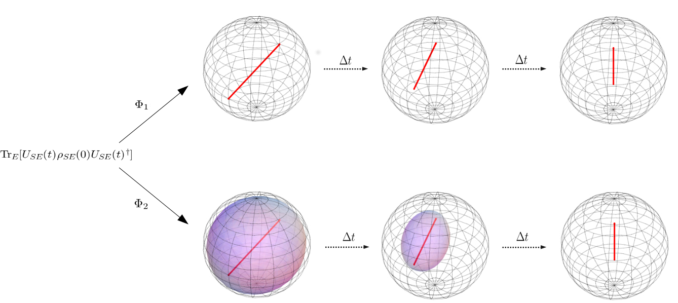
Figure 1: Schematic illustration of the different action of the maps $\Phi_{1}(t)$ and $\Phi_{2}(t)$ defined in Eq. (28) and Eq. (29) respectively. The different plots show the transformed Bloch sphere at subsequent times for the choice $y=\frac{1}{5}$ and $\chi=-\frac{2}{5}$ in Eq. (35). The commutative compatibility domain is here given by a diameter of the sphere, which transforms in the same way under the action of the maps, while the transformation of the rest of the sphere does depend on the choice of extension.

It is interesting to compare these results with the analysis performed in Rodriguez2008a (8), where the problem of obtaining a completely positive mapping starting from a correlated state was addressed for zero discord states. In particular the authors considered the state

$$\rho_{SE}=\frac{1}{4}[\mathbbm{1}_{S}\otimes\mathbbm{1}_{E}+y\sigma_{S}^{2}\otimes\mathbbm{1}_{E}-\chi\sigma_{S}^{2}\otimes\sigma_{E}^{3}],$$ (35)

which we recover upon setting

$$\{p_{1},\lambda_{+1},\lambda_{-1}\} \rightarrow \left\{\frac{1}{2},\frac{1}{2}\left(1-\frac{\chi}{1+y}\right),\frac{1}{2}\left(1+\frac{\chi}{1+y}\right)\right\}$$

$$\{p_{2},\lambda_{+2},\lambda_{-2}\} \rightarrow \left\{\frac{1}{2},\frac{1}{2}\left(1+\frac{\chi}{1-y}\right),\frac{1}{2}\left(1-\frac{\chi}{1-y}\right)\right\},$$ (36)

where the constraints $|y|\leqslant 1$ and $\chi^{2}\leqslant 1-y^{2}$ hold, and let it evolve according to Eq. (32). In particular by substituting the values Eq. (36) in the expression Eq. (50) one can obtain from Eq. (34) the corresponding expression for the Choi matrix, given in Eq. (54) of the Appendix. It can be noted that this matrix does not coincide with the result presented in Sec. 5 of Rodriguez2008a (8), despite the fact that the authors there advocate just one of the constructions that we used to come from a zero quantum discord state to the completely positive map, namely Eq. (29). The result can be understood as follows. The composition of any positive map, coming e.g. from a reduced dynamics as in Eq. (1), with a diagonalizing map as in Eq. (26) leads to a completely positive map. Indeed by composing a map with a diagonalizing map we obtain for the map a commutative domain, on which positivity is equivalent to complete positivity, independently of the choice of orthogonal projections $\{\Pi_{\varphi_{i}}\}_{i}$.

II.4 Reduced dynamics from discordant states

As simplest example of a completely positive map obtained starting from discordant states let us  consider $\mathcal{H}_{S}$ of dimension $n$ and take the state

$$\rho_{SE} = \sum_{i=1}^{n-2}p_{i}|\varphi_{i}\rangle\langle\varphi_{i}|\otimes\rho^{i}_{E}+p_{d}\sum_{k=1}^{3}\mu_{k}|\psi_{k}\rangle\langle\psi_{k}|\otimes\varrho_{E}^{k}$$ (37)

where introducing the two orthonormal states $\{|0\rangle,|1\rangle\}$, further orthogonal to $\{|\varphi_{i}\rangle\}_{i=1,\ldots,d}$, we have $\left\{|\psi_{1}\rangle=|0\rangle,|\psi_{2}\rangle=|1\rangle,|\psi_{3}\rangle=|+\rangle\right\}$, with $|+\rangle=(|0\rangle+|1\rangle)/\sqrt{2}$ and $|-\rangle=(|0\rangle-|1\rangle)/\sqrt{2}$. The state $W$ can therefore be written

$$W = \left(\begin{array}[]{cc}\mu_{1}+\frac{\mu_{3}}{2}&\frac{\mu_{3}}{2}\\ \frac{\mu_{3}}{2}&\mu_{2}+\frac{\mu_{3}}{2}\end{array}\right),$$ (40)

and one can consider its spectral decomposition

$$W = \sum_{i=1,2}w_{i}|\phi_{i}\rangle\langle\phi_{i}|,$$ (41)

leading according to Eq. (16) to a set of six Kraus operators. For the simplest case of a uniform probability distribution, so that $\mu_{k}=\frac{1}{3}$ for all $k$, we have $\{|\phi_{1}\rangle=|+\rangle,|\phi_{2}\rangle=|-\rangle\}$ together with $\{w_{1}=2/3,w_{2}=1/3\}$. This choice of parameters allows us to make direct contact with the example considered in Brodutch2013a (11). We obtain in particular the set of Kraus operators $K_{jk}=\sqrt{\lambda_{kj}}|\psi_{k}\rangle\langle\phi_{j}|$

$$K_{+0}=\sqrt{\frac{1}{4}}|0\rangle\langle+|\qquad K_{+1}=\sqrt{\frac{1}{4}}|1\rangle\langle+|\qquad K_{++}=\sqrt{\frac{1}{2}}|+\rangle\langle+|$$ (42)

$$K_{-0}=\sqrt{\frac{1}{2}}|0\rangle\langle-|\qquad K_{-1}=\sqrt{\frac{1}{2}}|1\rangle\langle-|\qquad K_{-+}=0$$ (43)

which leave $W$ defined in Eq. (41) invariant according to

$$\sum_{k=1,2,3}\sum_{j=\pm}K_{jk}WK_{jk}^{\dagger}=W,$$

and leading according to the general theory to the positive operator-valued measure $\{\Pi_{\varphi_{i}},K_{jk}^{\dagger}K_{jk}\}_{i=1,\cdots,n-2;j=\pm;k=1,2,3}$. Note that this set of Kraus operators does not coincide with those exhibited in Brodutch2013a (11). This fact can again be traced back to the non uniqueness in the construction of the completely positive map. Indeed while the action of the map on the set of operators commuting with the marginal of Eq. (37) is uniquely defined, the extension to the whole space of statistical operators can be obtained in many ways, still preserving complete positivity. In particular it can be seen that the set $\{K_{jk}\}$ with $K_{jk}=\sqrt{\mu_{k}}|\chi_{j}\rangle\langle\psi_{k}|$ still obeys Eq. (17) for any collection $\{\chi_{j}\}_{j}$ of normalized but not necessarily orthogonal states such that $\sum_{j}|\chi_{j}\rangle\langle\chi_{j}|$ acts as the identity on the space spanned by $\{\phi_{i}\}_{i=1,2}$.

III Discussion

The possibility to consider a reduced dynamical description for a given set of quantum degrees of freedom interacting with some external environment provides a very convenient way to account for the observed dynamics of such degrees of freedom. In this respect open quantum system theory has led to a satisfactory explanation of various physical phenomena and its general framework provides viable schemes to cope with the description of dissipation and decoherence effects in many different fields. However according to the general theory it is clear how to obtain a reduced dynamics only in the presence of an initially factorized system-environment state, a condition which cannot always be considered as realistic in the presence of strong coupling. The extension of the formalism to include correlated initial states however appears to be non trivial and not always bears with itself the desired properties. In this article we have provided a general construction of dynamical map, for an arbitrary unitary interaction between system and environment, for a class of correlated states possibly including states with non zero discord. This result encompasses previous work and put it within a unified viewpoint. It also shows that the definition of a reduced dynamical map in the case of correlated states is linked to the introduction of a set of Kraus operators building up a positive operator-valued measure which leaves the reduced system state invariant. The key observation lies in the characterization of the set of reduced states compatible with given correlations. If this compatibility domain is made up of commuting states, exploiting the identification between positivity and complete positivity on such sets one can actually introduce well defined evolution maps. The latter can also be extended to the whole set of statistical operators, still retaining the property of complete positivity. However such extensions are generally highly non unique, as we have explicitly pointed out by means of example. This point, to the bet of our knowledge, has yet not been put into the due evidence in the literature, and has allowed us to better clarify previous special results Rodriguez2008a (8, 11). Indeed while coinciding in their action on the compatibility domain, they generally transform in a different way states outside this domain. Moreover outside the compatibility domain they do not necessarily act as the identity at the initial time, thus describing a kind of initial slippage. The obtained picture, while elucidating a few basic points, and providing a constructive approach, further shows that extension of such maps beyond their natural domain, while preserving complete positivity is not necessarily of direct physical relevance.

It remains an open and relevant question whether the formalism can also be extended to states containing quantum correlations in the form of entanglement.

Appendix A Construction of the mappings $\Phi_{1}$ and $\Phi_{2}$

We now consider how to explicitly obtain the completely positive maps $\Phi_{1}(t)$ and $\Phi_{2}(t)$ starting from the correlated state considered in Eq. (31), according to the dynamics described by Eq. (32). In order to identify the completely positive maps Eq. (28) and Eq. (29) we exploit a matrix representation of these maps Heinosaari2011 (39), given by

$$\Lambda^{1,2}_{ij,kl}(t) = \langle i|\Phi_{1,2}(t)[|k\rangle\langle l|]|j\rangle,$$ (44)

where the indexes take on the values 0 and 1. To actually evaluate the matrix elements we observe that the unitary evolution given by Eq. (32) can be written, up to an irrelevant phase factor, in the form

$$U_{SE}(t)=\cos(2\omega t)\mathbbm{1}_{S}\otimes\mathbbm{1}_{E}-\frac{i}{2}\sin(2\omega t)\sum_{j=0}^{3}\sigma_{S}^{j}\otimes\sigma_{E}^{j}.$$ (45)

A straightforward but lengthy calculation then leads to the explicit expression for the matrices $\Lambda^{1,2}_{ij,kl}(t)$, which act identically on states diagonal in the eigenbasis of $\sigma_{y}$, while transforming in a different way system states diagonal in different bases. In particular they generally do not act as the identity map for $t=0$.

We start considering the matrix associated to $\Phi_{2}(t)$. We need to evaluate the operators

$$M_{\gamma\boldsymbol{\alpha}}(t) = \sum_{i=1,2}M_{\gamma\alpha_{i}}(t)$$

$$= \sum_{i=1,2}\sqrt{\lambda_{\alpha_{i}}}\langle\gamma|U_{SE}(t)|\alpha_{i}\rangle\Pi_{\varphi_{i}},$$

where $\{\Pi_{\varphi_{i}}\}_{i}$ now denote the projections $\{\Pi_{S}^{i}\}_{i=1,2}$ on the eigenvectors of $\sigma_{y}$ and $\{|\alpha_{i}\rangle\}_{i}$ are actually independent from $i$, since both environmental statistical operators are diagonal in the computational basis. We obtain

$$\langle 0|U_{SE}(t)|0\rangle = \cos(2\omega t)\mathbbm{1}_{S}-i\sin(2\omega t)|0\rangle\langle 0|$$

$$\langle 0|U_{SE}(t)|1\rangle = -i\sin(2\omega t)\sigma_{S}^{-}$$

$$\langle 1|U_{SE}(t)|0\rangle = -i\sin(2\omega t)\sigma_{S}^{+}$$

$$\langle 1|U_{SE}(t)|1\rangle = \cos(2\omega t)\mathbbm{1}_{S}-i\sin(2\omega t)|1\rangle\langle 1|,$$ (47)

where we have denoted $C(t)=\cos(2\omega t)$, $S(t)=\sin(2\omega t)$ and defined the raising and lowering operators according to $\sigma_{S}^{+}=|0\rangle\langle 1|$ and $\sigma_{S}^{-}=|1\rangle\langle 0|$, leading according to Eq. (30) to

$$M_{000} = C(\sqrt{\lambda_{+1}}\Pi_{S}^{1}+\sqrt{\lambda_{+2}}\Pi_{S}^{2})-iS\Sigma_{+}|0\rangle\langle 0|-S\Delta_{+}\sigma_{S}^{+}$$

$$M_{011} = -iS\Sigma_{-}\sigma_{S}^{-}-S\Delta_{-}|1\rangle\langle 1|$$

$$M_{100} = -iS\Sigma_{+}\sigma_{S}^{+}+S\Delta_{+}|0\rangle\langle 0|$$

$$M_{111} = C(\sqrt{\lambda_{-1}}\Pi_{S}^{1}+\sqrt{\lambda_{-2}}\Pi_{S}^{2})-iS\Sigma_{-}|1\rangle\langle 1|+S\Delta_{-}\sigma_{S}^{-},$$ (48)

and used the notation $M_{\gamma\boldsymbol{\alpha}}(t)\rightarrow M_{\gamma\alpha_{1}\alpha_{2}}$. One can directly check the identity $\sum_{\gamma,\boldsymbol{\alpha}}M_{\gamma\boldsymbol{\alpha}}(t)^{{\dagger}}M_{\gamma\boldsymbol{\alpha}}(t)=\mathbbm{1}_{S}$, granting trace preservation of the map. Computing the action of the map on the computational basis by evaluating $\sum_{\gamma,\alpha}M_{\gamma\boldsymbol{\alpha}}(t)|k\rangle\langle l|M_{\gamma\boldsymbol{\alpha}}(t)^{\dagger}$ and taking the matrix elements one can find the matrix $\Lambda^{2}_{ij,kl}(t)$

$$\Lambda^{2}=\left(\begin{array}[]{cccc}C^{2}\chi_{+}+S^{2}\mu_{+}&SC(\varkappa_{-}-\varkappa_{+})&SC(\varkappa_{-}-\varkappa_{+})&C^{2}\kappa_{+}+S^{2}\mu_{-}\\ 2iS^{2}\varkappa_{+}&\begin{array}[]{c}C^{2}\chi_{+}-iCS\chi_{-}\end{array}&\begin{array}[]{c}-C^{2}\kappa_{+}-iCS\kappa_{-}\end{array}&2iS^{2}\varkappa_{-}\\ -2iS^{2}\varkappa_{+}&-C^{2}\kappa_{+}+iCS\kappa_{-}&\begin{array}[]{c}C^{2}\chi_{+}+iCS\chi_{-}\end{array}&-2iS^{2}\varkappa_{-}\\ \begin{array}[]{c}C^{2}\kappa_{+}+S^{2}\mu_{+}\end{array}&SC(\varkappa_{-}-\varkappa_{+})&SC(\varkappa_{-}-\varkappa_{+})&C^{2}\chi_{+}+S^{2}\mu_{-}\end{array}\right),$$ (49)

upon introducing the notation

$$\varkappa_{\pm} = \Sigma_{\pm}\Delta_{\pm}$$

$$\mu_{\pm} = \Sigma^{2}_{\pm}+\Delta^{2}_{\pm}$$

$$\chi_{\pm} = \Sigma^{2}_{+}\pm\Sigma^{2}_{-}$$

$$\kappa_{\pm} = \Delta_{+}^{2}\pm\Delta^{2}_{-},$$ (50)

where

$$\Sigma_{\pm} = \frac{\sqrt{\lambda_{\pm 1}}+\sqrt{\lambda_{\pm 2}}}{2}$$

$$\Delta_{\pm} = \frac{\sqrt{\lambda_{\pm 1}}-\sqrt{\lambda_{\pm 2}}}{2},$$ (51)

so that the constraints $\mu_{-}+\mu_{+}=1$ and $\kappa_{+}+\varkappa_{+}=1$ are fulfilled.

Appendix B Choi matrices

Given this matrix representation complete positivity can be checked using the fact that the Choi matrices $\Phi^{1,2}_{\operatorname{Choi}}(t)$ associated to the two maps are simply obtained by a suitable transposition of indexes

$$\Phi^{1,2}_{\operatorname{Choi}}(t) = \Lambda^{1,2}_{ik,jl}(t).$$ (52)

The expression of $\Phi^{2}_{\operatorname{Choi}}(t)$ is given in Eq. (34), and its positivity can be directly checked.

The matrix representation of $\Lambda^{1}_{ij,kl}(t)$ can be more simply obtained exploiting the result Eq. (27), and therefore evaluating the action of the Kraus operators $M_{\gamma\boldsymbol{\alpha}}(t)$ on the elements $\{\Pi^{1}_{S}|i\rangle\langle j|\Pi^{1}_{S}+\Pi^{2}_{S}|i\rangle\langle j|\Pi^{2}_{S}\}_{i,j=0,1}$, leading to the result

$$\Lambda^{1}=\frac{1}{2}\left(\begin{array}[]{cccc}C^{2}+2S^{2}\mu_{+}&2SC(\varkappa_{-}-\varkappa_{+})&2SC(\varkappa_{-}-\varkappa_{+})&C^{2}+2S^{2}\mu_{-}\\ 4iS^{2}\varkappa_{+}&\begin{array}[]{c}C^{2}-iCS(\mu_{+}-\mu_{-})\end{array}&-C^{2}-iCS(\mu_{+}-\mu_{-})&4iS^{2}\varkappa_{-}\\ -4iS^{2}\varkappa_{+}&-C^{2}+iCS(\mu_{+}-\mu_{-})&C^{2}+iCS(\mu_{+}-\mu_{-})&-4iS^{2}\varkappa_{-}\\ C^{2}+2S^{2}\mu_{+}&2SC(\varkappa_{-}-\varkappa_{+})&2SC(\varkappa_{-}-\varkappa_{+})&C^{2}+2S^{2}\mu_{-}\end{array}\right),$$ (53)

which further leads to the associated Choi matrix $\Phi^{1}_{\operatorname{Choi}}(t)$ given in Eq. (33).

We note in particular that for the choice of system-environment state given by Eq. (36) upon substituting in Eq. (50) one recovers the following Choi matrix Eq. (34) associated to $\Phi_{2}(t)$

$$\Phi_{\operatorname{Choi}}=\frac{1}{2}\left(\begin{array}[]{cccc}\begin{array}[]{c}C^{2}(1+a_{+})\\ +S^{2}(1+yb)\end{array}&SCb&-iS^{2}b&\begin{array}[]{c}C^{2}(1+a_{+})\\ -iCS(yb-a_{-})\end{array}\\ SCb&\begin{array}[]{c}C^{2}(1-a_{+})\\ +S^{2}(1-yb)\end{array}&\begin{array}[]{c}-C^{2}(1-a_{+})\\ -iCS(yb+a_{-})\end{array}&iS^{2}b\\ iS^{2}b&\begin{array}[]{c}-C^{2}(1-a_{+})\\ +iCS(yb+a_{-})\end{array}&\begin{array}[]{c}C^{2}(1-a_{+})\\ +S^{2}(1+yb)\end{array}&SCb\\ \begin{array}[]{c}C^{2}(1+a_{+})\\ +iCS(yb-a_{-})\end{array}&-iS^{2}b&SCb&\begin{array}[]{c}C^{2}(1+a_{+})\\ +S^{2}(1-yb)\end{array}\end{array}\right),$$ (54)

where to simplify notation we have set

$$a_{\pm} = \frac{1}{2}\left(\sqrt{\frac{1-(y+\chi)^{2}}{1-y^{2}}}\pm\sqrt{\frac{1-(y-\chi)^{2}}{1-y^{2}}}\right)$$

$$b = \frac{\chi}{1-y^{2}}.$$

References

• (1) H.-P. Breuer and F. Petruccione, The Theory of Open Quantum Systems (Oxford University Press, Oxford, 2002)
• (2) U. Weiss, Quantum Dissipative Systems, 2nd edn. (World Scientific, Singapore, 1999)
• (3) V. Gorini, A. Kossakowski, and E. C. G. Sudarshan, J. Math. Phys. 17, 821 (1976)
• (4) G. Lindblad, Comm. Math. Phys. 48, 119 (1976)
• (5) D. Bondar, R. Cabrera, A. Campos, S. Mukamel, and H. A. Rabitz, arXiv:1412.1892 (2014)
• (6) A. Rivas, S. F. Huelga, and M. B. Plenio, Rep. Prog. Phys. 77, 094001 (2014)
• (7) H.-P. Breuer, E.-M. Laine, J. Piilo, and B. Vacchini, Rev. Mod. Phys. 88, 021002 (2016)
• (8) C. A. Rodriguez-Rosario, K. Modi, A. Kuah, A. Shaji, and E. C. G. Sudarshan, J. Phys. A: Math. Gen. 41, 205301 (2008)
• (9) A. Shabani and D. A. Lidar, Phys. Rev. Lett. 102, 100402 (2009)
• (10) C. A. Rodríguez-Rosario, K. Modi, and A. Aspuru-Guzik, Phys. Rev. A 81, 012313 (2010)
• (11) A. Brodutch, A. Datta, K. Modi, A. Rivas, and C. A. Rodríguez-Rosario, Phys. Rev. A 87, 042301 (2013)
• (12) K. K. Sabapathy, J. S. Ivan, S. Ghosh, and R. Simon, arXiv:1304.4857 (2013)
• (13) L. Liu and D. M. Tong, Phys. Rev. A 90, 012305 (2014)
• (14) J. Dominy, A. Shabani, and D. Lidar, Quant. Inf. Proc. 15, 465 (2016)
• (15) H. Grabert, P. Schramm, and G. Ingold, Phys. Rep. 168, 115 (1988)
• (16) A. R. U. Devi, A. K. Rajagopal, and Sudha, Phys. Rev. A 83, 022109 (2011)
• (17) K. Modi, Scientific Reports 2, 581 (2012)
• (18) V. Ignatyuk and V. Morozov, Condens. Matter Phys. 16, 34001 (2013)
• (19) H.-P. Breuer, J. Gemmer, and M. Michel, Phys. Rev. E 73, 016139 (2006)
• (20) P. Pechukas, Phys. Rev. Lett. 73, 1060 (1994)
• (21) R. Alicki, Phys. Rev. Lett. 75, 3020 (1995)
• (22) P. Stelmachovic and V. Buzek, Phys. Rev. A 64, 062106 (2001)
• (23) F. Buscemi, Phys. Rev. Lett. 113, 140502 (2014)
• (24) M. Nielsen and I. Chuang, Quantum Computation and Quantum Information (Cambridge University Press, Cambridge, 2000)
• (25) A. S. Holevo, Statistical Structure of Quantum Theory, Vol. m 67 of Lecture Notes in Physics (Springer, Berlin, 2001)
• (26) W. F. Stinespring, Proceedings of the American Mathematical Society 6, 211 (1955)
• (27) M. Takesaki, Theory of Operator Algebras I (Springer, Berlin, 2002)
• (28) F. Strocchi, An introduction to the mathematical structure of quantum mechanics (World Scientific, 2005)
• (29) H. Ollivier and W. H. Zurek, Phys. Rev. Lett. 88, 017901 (2001)
• (30) L. Henderson and V. Vedral, Journal of Physics A: Mathematical and General 34, 6899 (2001)
• (31) K. Kraus, States, Effects and Operations: Fundamental Notions of Quantum Theory (Springer, Berlin, 1983)
• (32) E. Schrödinger, Proceedings of the Cambridge Philosophical Society 31, 555 (1935)
• (33) N. Gisin, Helv. Phys. Acta 62, 363 (1989)
• (34) L. P. Hughston, R. Jozsa, and W. K. Wootters, Phys. Lett. A 183, 14 (1993)
• (35) M. Gessner and H.-P. Breuer, Phys. Rev. Lett. 107, 180402 (2011)
• (36) M. Gessner and H.-P. Breuer, Phys. Rev. A 87, 042107 (2013)
• (37) M. Gessner, M. Ramm, T. Pruttivarasin, A. Buchleitner, H.-P. Breuer, and H. Häffner, Nature Physics 10, 105 (2014)
• (38) S. Cialdi, A. Smirne, M. G. A. Paris, S. Olivares, and B. Vacchini, Phys. Rev. A 90, 050301 (2014)
• (39) T. Heinosaari and M. Ziman, The Mathematical Language of Quantum Theory (Cambridge University Press, Cambridge, 2011)
Acknowledgements
B.V. acknowledges support from the EU Collaborative Project QuProCS (Grant Agreement 641277) and by the Unimi TRANSITION GRANT - HORIZON 2020.