Yarrp’ing the Internet: Randomized High-Speed Active Topology Discovery

Abstract

Obtaining a “snapshot” of the Internet topology remains an elusive task. Existing active topology discovery techniques and systems require significant probing time – time during which the underlying network may experience transient dynamics. This work considers how active probing can gather the Internet topology in minutes rather than days. Conventional approaches to active topology mapping face two primary speed and scale impediments: i) per-trace state maintenance; and ii) a low-degree of parallelism. Based on this observation, we develop Yarrp (Yelling at Random Routers Progressively), a new traceroute technique designed for high-rate, Internet-scale probing. Yarrp is stateless, reconstituting all necessary information from ICMP replies as they arrive asynchronously. To avoid overloading routers or links with probe traffic, Yarrp randomly permutes an input $IP\times TTL$ space. We run Yarrp at $100Kpps$, a rate at which the paths to all IPv4 /24’s can be mapped in approximately one hour from a single vantage point. We compare Yarrp against existing systems, and present examples of topological dynamics exposed via the high sampling rates Yarrp enables.

1 Introduction

Network and security researchers rely on topological maps of the logical Internet to address problems ranging from critical infrastructure protection to policy. Production active measurement systems that continually gather and curate Internet topology, e.g. [22, 17], are thus important to many longitudinal analyses and to shedding light on network events of interest.

Obtaining IP, router, and provider-level network topologies has been a continual research focus for more than two decades [16, 19, 26, 22]. While significant progress has been made, topology mapping at Internet scale remains a challenge. Both the accuracy of the inferred network topologies [29], and the speed at which they can be recovered [12, 6], present obstacles to current mapping efforts. Although systems that sample paths at a rate inversely proportional to their stability have shown promise, even state-of-the-art techniques to predict path changes are relatively inaccurate [11]. In this work, we focus on the speed and scale of Internet-wide active topology mapping.

Given its scale, experience and popular belief dictates that obtaining even partial Internet topologies via active network probing is a time-intensive process. For instance, CAIDA’s Archipelago (Ark) [17] system uses dozens of vantage points and at least a day to traceroute to a single address in each routed /24 IPv4 prefix. A recent topology cycle gathered by Ark from April, 2016 [8] sent approximately 11M traceroutes from 37 monitors over the course of 31 hours in order to discover $\approx$1M distinct router interfaces, and $\approx$2M links.

We re-examine the assumed fundamental limits of active topology mapping to consider whether probing can be performed in minutes rather than hours. Taking inspiration from recent stateless and randomized high-speed scanners, e.g. ZMap [13] and masscan [14], we create Yarrp (Yelling at Random Routers Progressively).

To facilitate high-probing rates, Yarrp is stateless, reconstituting all necessary information from replies as they arrive asynchronously. To avoid overloading routers or links, Yarrp randomly permutes its input $IP\times TTL$ space when probing. Yarrp is thus well-suited for Internet-scale studies. Our contributions include:

1. Development of Yarrp, a publicly available tool [5] that permits rapid active network topology discovery. We run Yarrp at $100Kpps$ to discover more than 400,000 router interfaces in under 30 minutes.

2. A comparison of Yarrp and CAIDA’s existing production topology collection platform, showing recall and speed differences.

3. As an application of rapid topology discovery, we conduct successive topology snapshots separated by a small time delta and characterize the distribution and causes of observed path differences.

2 Background

Traditional traceroute [18] obtains the sequence of router interface IP addresses along the forward path to a destination by sending probe packets with varying time to live (TTL) values and examining the ICMP responses. By maintaining the transmission timestamp of each probe, traceroute can report the round trip time (RTT) from the source to each responsive hop. Modern traceroute implementations send batches of concurrent probes to lower tracing time, e.g. Linux defaults to 16 simultaneous probes. In order to match probes to the ICMP TTL exceeded responses they generate, the probe must include unique identifiers that are returned as part of the ICMP quotation [23]. Because the quote is only required to copy the first 28 bytes of the packet that induced the expiry message [3], traceroute typically relies on the first 8 bytes of the transport-layer header to match responses to probes.

While various improvements have been proposed and implemented, the core behavior of traceroute – and large scale active topology scanning – remains largely unchanged. To prevent false inferences due to load-balanced paths, Augustin et al.created Paris traceroute [2]. To reduce unnecessary probing, Donnet et al.developed Doubletree [12], a modified traceroute that begins probing from a likely path midpoint outward until it reaches previously discovered hops. Similarly, [6, 4] proposed several topology primitives empirically shown to reduce the volume of probing while maintaining or increasing topological discovery. DTrack [11] and Sibyl [10] seek to optimize active probing by making predictions over historical measurements, yet are still constrained by traditional traceroute techniques.

CAIDA’s production Ark infrastructure [17] uses Scamper [21] to perform continual Internet-wide probing [8]. Scamper implements both Doubletree and Paris traceroute, has an open API, can maintain a configurable probing rate, and can be controlled remotely.

Traceroute was originally designed as a tool for network administrators to diagnose a small number of paths, not as a means to gather snapshots of the entire Internet topology [18, 19]. Fundamentally, traceroute and its variants all have two related properties that limit their scalability and speed. They:

• Maintain state for each outstanding probe sent, including some identifier and origination time.

• Are sequential, probing all hops along the path to a destination. While some tools (e.g. scamper) can traceroute to multiple targets, this parallelism is path specific.

In contrast, Yarrp is designed to be stateless and random – probing different portions of many different paths simultaneously. This allows Yarrp to send probes at a high per-packet rate, while spreading the load among many destination networks to avoid concentrating load on particular paths, links or routers, thereby avoiding anomaly alarms or ICMP rate limiting.

3 Yarrp Design

The high-level idea of Yarrp is: i) randomization of the probing order of the domain of network range(s) and TTLs; and ii) stateless operation, whereby all necessary state is encoded into the probes such that it can be recovered from the ICMP replies. As with ZMap, Yarrp uses independent send and receive threads, where the sender uses raw sockets while the receiver thread is implemented using libpcap. Yarrp is written in C++ (approximately 2,500 SLOC), is portable to a variety of UNIX-like platforms, and is publicly available [5].

3.1 Pseudo-random Probing Order

Existing traceroute techniques probe all hops along a path to a destination in sequence. Instead, we employ a keyed block cipher to provide a bijection over the input domain of target IPs and TTLs ($D=IPs\times TTLs$). This means, for example, that Yarrp may send a probe to IP address $A$ with $TTL=12$, then $B$ with $TTL=3$, then $C$ with $TTL=20$, and so on until the entire space of $TTLs$ for each target $IP$ is covered. To an outside observer, the probed addresses appear to be random.

The symmetric RC5 block cipher with a 32-bit block size is fast and a natural fit for our application. With key $k$, Yarrp encrypts the sequence $i=0,1,\ldots,|D|-1$ where bits of each ciphertext $C_{i}=RC5_{k}(i)$ determine the target IP address and TTL to probe. In this way, Yarrp randomizes the order of probed $\langle targetIP,TTL\rangle$. Yarrp can permute arbitrarily large or small IPv4 address and TTL domains, or can permute the order of specific targets read from a file. Depending on the size of the domain, we switch between either a prefix-cipher or cycle-walking cipher, as described in [7].

To facilitate comparison with CAIDA’s IPv4 topology dataset [8], Yarrp has a mode that probes a random address in each IPv4 24-bit subnet – this mimics the targets selected in a full cycle of CAIDA’s probing. Here, Yarrp encrypts each $i=0,\ldots,2^{24}-1$ with key $k$. For $C_{i}=RC5_{k}(i)$, Yarrp probes the IPv4 address $C_{i}[0\mathbin{:}23]*2^{8}+(C_{i}[0:7]+C_{i}[8:15]+C_{i}[16:23])\%256$ with TTL $C_{i}[24\mathbin{:}31]$. In this fashion, we permute through the space of $2^{24}$ possible /24s, and construct the least-significant octet as a function of the subnet such that the same random address in each /24 is used as the destination for each TTL.

An advantage of Yarrp’s randomization method is that the probing work can easily be distributed among multiple vantage points with negligible coordination or communication overhead. We discuss distributed Yarrp as a future enhancement in §5.

3.2 Stateless Operation

Existing traceroute techniques require state to match ICMP replies to probes. In contrast, Yarrp does not require state. We overload various fields in the probe packets with specific values such that we can reconstruct the corresponding probe’s destination, transmission time, and originating TTL from within the quote of the ICMP TTL exceeded messages.

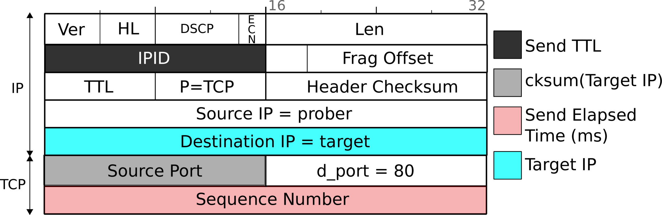
Figure 1: Yarrp encodes information in the IP and TCP fields of outgoing probe packets in order to permit stateless operation.

Figure 1 depicts the TCP/IP header fields we utilize. We encode the TTL with which the packet was sent in the IPID and the elapsed time in the TCP sequence number. We use elapsed time rather than e.g. Unix time in order to maintain millisecond resolution with only a 32-bit field. Yarrp can also encode microsecond resolution, so long as the expected duration of a probing run is less than $2^{32}/1\times 10^{6}\approx$4300 seconds. The destination TCP port is fixed to port 80 to facilitate firewall traversal, while we populate the source TCP port with the checksum of the target IP address. In this fashion, we can detect instances where the destination IP address is modified enroute, a phenomenon Malone and Luckie observe in 2% of their results [23].

In order to properly accommodate load-balanced paths, which are common in the Internet, we ensure that, for a given destination, certain fields remain fixed for all TTL probe values. For instance, although the TCP source port changes, it is a function of the destination IP address and therefore will contain the same value for all probes sent toward the destination. This design allows us to maintain the benefits of Paris traceroute [2].

When ICMP TTL exceeded messages arrive, we examine the included quotation to recover the destination probed, the originating TTL (hop), responding interface at that hop, and compute the RTT by taking the difference of the packet arrival time and the probe origination time as encoded in the quoted TCP sequence number. These values can be computed from the minimum 28 bytes of required quotation [3].

Yarrp can source either TCP SYN or ACK probes. While SYN probes can permit middlebox traversal, we use the ACK-only mode to avoid alarms triggered by large volumes of SYN traffic. We discuss our use of high-rate TCP ACK probing in §3.5, and outline a means to use ICMP and UDP probes in future work in §5.

3.3 Challenges

The benefits of Yarrp’s design come with several concomitant challenges, namely: i) reconstructing the unordered responses into paths, ii) knowing when to stop probing, and iii) avoiding unnecessary probing.

In following with Yarrp’s stateless nature, ICMP responses are decoded as they arrive and written sequentially to a structured output file. Each entry in the output file corresponds to an ICMP response. An entry includes the target IP address, originating TTL, responding router interface IP address, RTT, and meta-data such as timestamps, IPID, response TTL, packet sizes, and DSCP markings. Because of the inherently random probing, the entries for each hop along a path to a given destination will be unordered and intermixed with other responses in the Yarrp output file. We must therefore reconstruct complete paths by parsing the entire output file and maintaining state for each destination. While this is a memory and time-intensive task, the key point is that it can be performed off-line. In this fashion, we decouple probing from path reconstruction to permit the probing to be as fast as possible. Included in the Yarrp distribution [5] is a yrp2warts Python script that performs this off-line conversion into the standard warts [21] binary trace format.

A practical consequence of Yarrp’s randomization and lack of state is that its probing behavior does not depend on the received responses. Thus, Yarrp cannot stop probing once it reaches the destination or when the path contains a sequence of unresponsive hops (the so-called “gap limit”). To better understand the optimal range of TTLs to probe (from the possible space 1-255), we examine the results from a complete cycle of Ark probing from January, 2016 [8]. We seek to determine, across each of the Ark vantage points, the number of unique router interfaces discovered at each TTL.

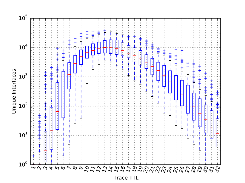
Figure 2: Distribution of interfaces discovered across Ark vantage points in a single cycle as a function of TTL (path depth). The red line indicates the median value among vantage points.

Figure 2 shows the inter-quartile range of the number of distinct interfaces found as a function of TTL for each of the vantage points; the red line in the boxplot displays the median number of interfaces per TTL among each vantage point. Because of the Internet’s tree-like structure, the first few hops reveal only a small number of interfaces regardless of the destination probed. The bulk of the interfaces are found between TTLs 10 to 16, with an inflection point around a TTL of 14. The amount of discoverable topology beyond a TTL of 32 is negligible (note the log scale y-axis). As a result, Yarrp defaults to probing TTLs 1 to 32 to minimize unnecessary probing while exploring the majority of the space.

For many destinations Yarrp will perform more probing than traditional traceroute methods. This is both an advantage and a disadvantage: we show in §3 that discoverable topology exists beyond multiple unresponsive hops (where existing methods terminate early).

3.4 Optimizations

In environments sensitive to probing volume, several optimizations can substantially decrease unnecessary probing at the expense of maintaining some state. This subsection discusses optimizations to the base Yarrp design to enable different tradeoffs.

First, Yarrp can read a BGP routing table of network prefixes and build a longest-match Patricia trie [25]. When iterating through the entire permuted IPv4 space, Yarrp can skip destinations that are not routed. Based on current global BGP routing tables [1], this optimization avoids probing approximately 1.5B IP addresses (35% of the 32-bit space) that are unlikely to return useful results. Note that the memory required to maintain the BGP table is constant during a probing run (amounting to approximately 300MB during runtime). In our experiments, these lookups in the Patricia trie did not prevent Yarrp from running at over $100kpps$.

Second, the tree-like structure of the network implies that the set of interfaces near to the vantage point is small relative to the universe of router interfaces [12]. In Figure 2 for instance, all of the traces have a single first hop in common and orders of magnitude fewer interfaces at hops 1-3 as compared to hops 13-15. To avoid rediscovering the same nearby router interfaces repeatedly, Yarrp can maintain state over the set of responding local “neighborhood” interface IP addresses at hops 1 through a run-time configurable $ttl_{nbrhd}$. For each TTL in the neighborhood, Yarrp maintains two timestamps: the last time a probe was sent with that TTL, and the last time a new interface at that depth replied. If no new interfaces have been discovered within the past $\eta=30$ seconds of probing, Yarrp skips future probes at that TTL. The yrp2warts script can then stitch together these missing hops. While the amount of state in neighborhood mode can grown unbounded, in practice it is small for small $ttl_{nbrhd}$, while avoiding substantial over-probing.

3.5 Ethical Concerns

High-speed probing invariably raises ethical concerns, as it increases the chance that traffic may be perceived as abusive. We follow the recommended guidelines for good Internet citizenship provided in [13] to mitigate the potential impact of our probing.

First, as described in §3.1, Yarrp’s pseudo-random probing order is designed to avoid overloading the networks it seeks to characterize. Second, Yarrp sends TCP ACK probes, which have been used in prior topology studies [20], and prevent end systems from attempting to negotiate a TCP connection (in contrast, the ZMap scanner sends TCP SYN packets). Unfortunately, Yarrp’s stateless nature implies that multiple probes, with different TTLs, may reach a single destination, an effect we analyze in §4.2.

We therefore make an informative web page accessible via the IP address of our prober, along with instructions for opting-out. Additionally, the reverse DNS record name indicates the research nature of the host. In this initial work, with Yarrp runs of 30 minutes or less, we did not receive any abuse reports or opt-out requests.

4 Results

This section examines results from running Yarrp on the Internet. We compare the topological recall against an existing production system and then analyze the discovery yield (i.e. the amount of new topology discovered over time). Finally, as an application of Yarrp’s probing speed, we gather three successive topology snapshotsto reveal instances of short-lived network dynamics.

4.1 Topological Recall

We empirically verify Yarrp’s topological recall by evaluating it against scamper [21]. From a single vantage point, we probe 67,045 destinations using Yarrp and scamper. We run scamper in Paris TCP ACK mode using port 80 in order to mimic Yarrp’s behavior and facilitate an unbiased comparison of topological recall between the two probing methods. From the Yarrp and scamper probing, construct graphs of interface nodes connected by edges when the interfaces appear in consecutive hops of a path. We ignore anonymous interfaces [15] such that the graph may be disconnected. Yarrp discovers 57,128 interfaces, 1.3% fewer than scamper’s 57,866 unique interfaces, and 67,563 edges (0.8% more than scamper). Manual investigation of the topologies reveals differences mainly attributable to load-balancing (because scamper and Yarrp use different headers, it is not possible to ensure that they traverse the same paths to destinations) and path changes. Empirically, our comparison demonstrates Yarrp’s ability to discover the responsive topology.

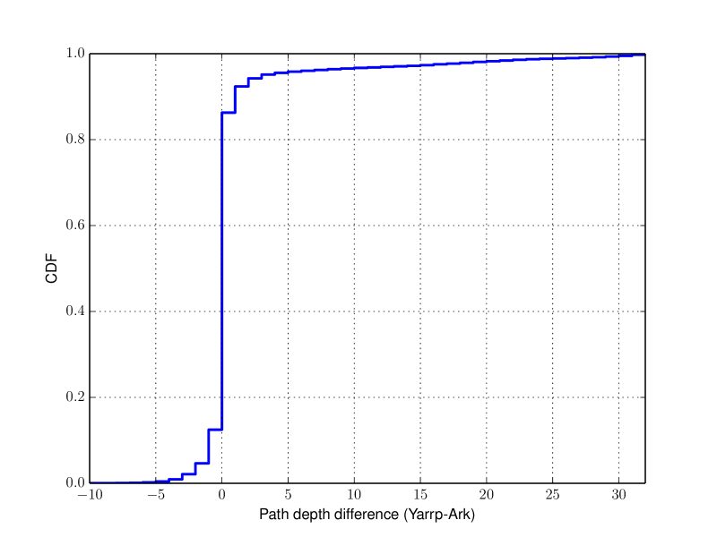
Figure 3: CDF of highest responding TTL difference (max(Yarrp)-max(Ark)) for Ark gap-limited traces (same dests. and vantage point).

Yarrp’s stateless nature implies that it probes all TTLs from 1 to 32, whereas Ark’s use of scamper ceases probing after encountering five unresponsive hops in a row. In the same CAIDA San Diego probing run, 39,613 traces stopped due to this gap-limit. For each of these gap-limit traces, we compute the difference of the highest responding TTL hop from Yarrp probing and the highest responding TTL from the Ark probing. Figure 3 shows the cumulative distribution of this difference among the gapped traces; a positive difference means that Yarrp discovered topology beyond the point where Ark stopped probing. For $\approx$88% of the traces, there is no difference. In 8% of the traces, Ark discovers one more hop than Yarrp. However, Yarrp discovers one additional hop in $\approx 6$% of the targets, and more than 5 additional hops in 4% of the cases.

4.2 Discovery Rate

A goal of Yarrp is rapid topological discovery. In this subsection, we look specifically at the ability to discover unique router interface addresses rapidly.

On May 10, 2016, we run Yarrp from a Northeast United States university vantage point at $\approx 100kpps$ and instruct it to perform the Ark-mode randomized probing of the globally routed IPv4 /24 prefixes. We limit Yarrp to this rate, and limit the duration of our experiment, per prior agreement with the local network administrator. The physical machine is a multi-core Intel L5640 processor running at 2.27GHz, with Yarrp running on an Ubuntu virtual machine allocated a single core. At this rate, the CPU utilization is $\approx$52%.

We enable the “neighborhood” optimization, as described in §3.4, as we are interested in finding as many distinct router interfaces as possible given the probing rate. Figure 4 displays the cumulative number of distinct router interfaces discovered as a function of time. As a basis of comparison, we also plot the number of unique interfaces found over time for a single vantage point (again, using data from the San Diego node of CAIDA’s continual /24 probing [8] on May 1, 2016).

CAIDA’s San Diego monitor discovers 12,568 unique interfaces in 1,500 seconds ($\approx 8$ per second). By contrast, Yarrp discovers 421,162 unique IPv4 interfaces in the same period, or approximately 280 distinct router interfaces a second. The number of interfaces found by Yarrp in less than 30 minutes equates to 42% of all unique interfaces discovered from all Ark monitors over the course of probing for more than a day.

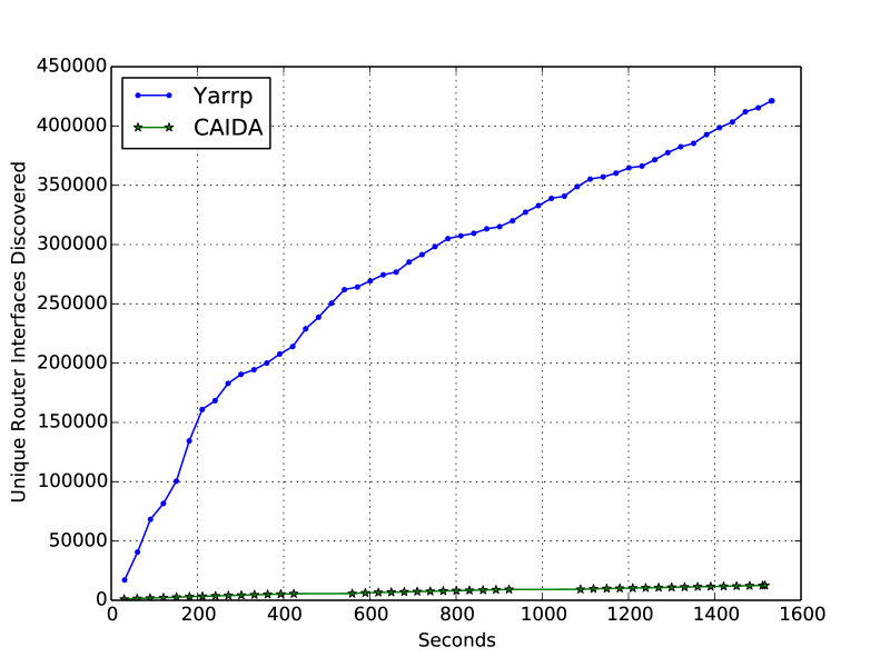
Figure 4: Unique router interface discovery rate: comparing Yarrp against CAIDA’s routed /24 probing from a single vantage point.

Recall that Yarrp decouples probing from topology reconstruction. Using a commodity 3.1GHz Intel Xeon processor, our unoptimized, single-threaded Python program (yrp2warts.py) converts our unordered high-speed Yarrp output trace of 6.8M destinations into an ordered warts-format file in 668 seconds. This empirical observation serves to provide an estimate of the wall-clock upper-bound required to obtain output identical to existing systems. We leave optimizing Yarrp topology reconstruction as future work.

Finally, in consideration of Yarrp’s stateless TCP probing, we examine the number and types of replies received during our probing run. Figure 5 displays the complementary cumulative distribution of hosts sending one or more non-TTL exceeded replies. We received approximately 1.2M TCP RST packets. 99.1% of the hosts that send a TCP RST packet sent 10 or fewer, indicating that these hosts received 10 or fewer probes. We received $\approx$95K host unreachable, and $\approx$63k communication prohibited ICMP messages. A very small number of hosts sent thousands of TCP RST packets; three three IP addresses within Wanadoo French Telecom send the majority of all RSTs. As Yarrp never sends more than 32 probes toward a given destination, a single IP sending a large number of RSTs is suggestive of a middlebox.

4.3 Short-Lived Dynamics

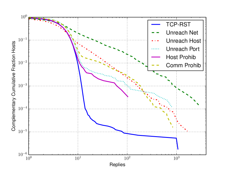
Figure 5: Number and type of non-TTL exceeded replies received per-host during large Yarrp probing run.

As an application of rapid topology discovery, we collect topology snapshots in rapid succession and analyze their properties and differences in this subsection.

We gather 67,045 target destinations from CAIDA’s May 1, 2016 topology probing from their San Diego monitor. Again using the east coast university vantage point, we run Yarrp to probe TTLs 1-32 for these same 67,045 targets. We run Yarrp at $\approx 4000pps$ and invoke Yarrp three times in succession with a minute pause in-between. In this way, each snapshot takes approximately 8 minutes to gather, and each is separated by a minute. The permutation key is the same for each snapshot, thus the random probing order is identical for each. We term the snapshots $S_{1},S_{2}$ and $S_{3}$ in chronological order.

The interface-level graph resulting from $S_{1}$ contains 39,968 interfaces and 46,721 edges, while $S_{2}$ has 40,038 interfaces and $46,773$ edges. $S_{3}$ contains $39,994$ interfaces and $46,749$ edges. To better understand the differences between snapshots, we perform a per-target path comparison. For each target in $S_{1}$, we compare the discovered path in $S_{1}$ to the path to that same target in $S_{2}$. We use the Levenshtein edit distance to measure the per-target path differences between snapshots. The edit distance is the minimum number of edits (insertions, substitutions, or deletions of router interfaces).

Note that inter-snapshot differences are not attributable to per-flow load balancing as Yarrp keeps the packet header fields which are used for load balancing constant for the same destination between snapshots (§3.2).

Additionally, to better understand the types of path changes, we count the frequency of each edit operation and missing hop substitutions. These missing hop operations are instances where the path contains a responsive router for a particular TTL for one snapshot, but no response at that TTL when probing the same destination in a subsequent snapshot. Such missing hops may be attributable to routers performing ICMP rate limiting, or may be due to packet loss.

A deeper analysis of the most frequent missing hops between $S_{1}$ and $S_{2}$ reveals that the large majority (92.2%) come from the first four hops within the local network of the vantage point. Specifically, 73% of the missing hops are due to the router at TTL 3, 18% are due to the router at TTL 1, and 1% are due to the router at TTL 4. In contrast, the router at TTL 2 always responds, suggest that some of the local routers implement ICMP rate limiting while one does not.

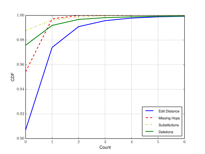
Figure 6: Cumulative fraction of measured paths versus pair-wise path edit distance between successive Yarrp topology snapshots.

Figure 6 displays the results of the edit distance comparison between $S_{1}$ and $S_{2}$, ignoring differences due to the vantage point’s local network (TTL $\leq 4$, as described above). The paths to approximately 91% of the destinations are identical between $S_{1}$ and $S_{2}$, while approximately 6% have a single hop difference. Less than 1% of the destinations show a difference of $\geq 2$ hop edits. Separated by the edit operation, $\approx$4% of the paths have 1 hop differences that are due to missing hops, 1% are hop deletions, and fewer than 1% are substitutions.

To understand the potential of rapidly collected topology snapshots, we manually investigate and highlight a path exhibiting a significant change between snapshots. Figure 7 shows, for each of the three snapshots, entirely different paths toward the destination 131.221.200.245 (in AS 262316). In $S_{1}$, the trace leaves our vantage point’s local network via AS3356 (Level 3), via AS10578 in $S_{2}$ (Internet 2 Northeast Gigapop), and AS174 (Cogent) in $S_{3}$. We manually confirm significant routing churn for the target’s prefix (131.221.200.0/22) evident in BGP updates archived by Routeviews [1]. During our snapshot collection, there were 176 BGP updates involving the target prefix, while there were no BGP updates for the same prefix in the prior 15-minute Routeviews BGP archive.

Similarly, we find short-lived dynamics within the core of the network in our snapshots. Figure 8 shows traces toward 129.232.142.175 (AS37153, in South Africa) traversing Level 3 (AS3356) and AS36351 before reaching AS37153 in $S_{1}$, then converging on a path via AS37179 rather than AS36351. Again, there are no BGP updates for 129.232.128.0/17 in the Routeviews archive 15 minutes prior, but 217 updates during, our probing.

While the exact cause of this short-lived routing change is unknown, the key point is that it would not have been discovered by the existing topology mapping systems. We further find intra-AS dynamics between paths to the same destination in our snapshots. These differences cannot be validated against available BGP updates visible at Routeviews, but suggest that Yarrp’s data-plane inferences may be complementary to techniques that rely on the visibility of dynamics within the control-plane. We leave a comprehensive analysis of the extent and duration of these short-lived dynamics exposed by Yarrp to future work.

     S1: .. 18.192.9.2 4.53.48.97 4.69.144.80 4.26.0.166 201.48.50.161  S2: .. 18.192.9.2 207.210.142.229 198.71.47.57 * 67.16.148.6 201.48.50.161  S3: .. 18.192.9.2 38.104.186.185 154.54.30.41 154.54.47.30 154.54.11.110     

Figure 7: Example of short-lived path dynamics observed near our vantage point via successive, rapidly collected topology snapshots.

5 Conclusions

Yarrp demonstrates a new technique for Internet-scale active probing that permits rapid collection of topology snapshots. Our hope is that Yarrp facilitates analyses not previously possible. For instance, Yarrp can enable a detailed longitudinal analysis of short-lived topology dynamics across the entire Internet in future work.

Yarrp is stable and the code is publicly available [5]. That said, there are several enhancements that would be valuable additions. First, Yarrp currently only supports IPv4 probing. Given the vastly larger IPv6 address space, and relative topological sparsity [24], adding IPv6 support to Yarrp could enable more complete maps of the IPv6 topology to be gathered. While the streamlined IPv6 headers prevent direct application of Yarrp’s IPv4 header encoding, the full packet quotation in ICMP6 permits more flexibility in recovering state and using different transport protocols.

Second, while Yarrp sends TCP probes, it is well-known that using different transport protocols yields different responses, due to security and policy filtering [20]. Adding ICMP and UDP probing to Yarrp requires utilizing different transport header fields to encode probe information, while maintaining the first four bytes constant to keep packets on a single load-balanced path. For UDP we expect to encode time into the length and checksum fields and include a payload that makes the checksum correct. For ICMP echo, we can encode the timestamp into the identifier and sequence number headers, but must include a payload that produces the same checksum for every packet toward a target.

Third, Yarrp’s stateless and asynchronous nature implies that a malicious actor could attempt to send bogus responses, while middleboxes are known to mangle packet headers [9, 23]. In the future, we wish to use a keyed cryptographic integrity function over multiple probe values. Instead of a simple checksum on the target IP address, we will populate the source port with the value of this keyed integrity check. Yarrp can then ensure that it both sent the original probe, and that the probe was not modified in-flight.

Fourth, while the headers used for load-balancing remain consistent for all probes toward a given destination, the ICMP responses that Yarrp elicits will have different checksums due to the quotation containing Yarrp’s timestamp. When a router with equal-cost paths back to the source must generate an ICMP response, it may choose a source interface based on the ICMP headers (including the ICMP checksum). Thus, a load-balancing router at a particular hop may respond with a different IP address between subsequent Yarrp traces. In future work we plan to address this subtlety.

Finally, an attractive feature of Yarrp’s design is the ability to easily randomize and distribute the probing to multiple vantage points with negligible coordination and communication overhead. Similar to the rapid scanning worm envisioned by Staniford et al., the permuted domain can be distributed [27]. While the entire domain can be subdivided among vantage points, doing so causes different vantage points to probe different TTLs for a given target. Instead, a simple scheme can distribute the probing while ensuring that all hops toward a target are probed from a consistent source. Each of $n$ vantage points permutes the same domain $D=IPs\times TTLs$. However, the $i$’th vantage point only sends a probe for addresses where $IP\%(n-1)==i$. For additional randomness, the IP may be hashed prior to this check. The potential speed improvement is linearly proportional then to the number of vantage points. Only the values $|D|$, $i$, and $key$ need be sent to each vantage point to distribute the permuted space and achieve complete randomized coverage. Given our empirical (and conservative) $100kpps$ Yarrp rate in this work, we estimate that it is possible to implement a distributed Yarrp among $\approx$128 vantage points to traceroute to every routed IPv4 address ($\approx 2^{31}$ targets) in approximately one hour. Yarrp may thus facilitate rapid collection of complete Internet snapshots in the future.

     S1: .. 4.69.166.5 212.113.14.82 50.97.19.43 5.10.118.137 159.8.138.4  S2: .. 4.69.166.5 4.69.167.82 50.97.19.43 41.84.12.81 41.66.132.246  S3: .. 4.69.166.5 4.69.167.82 212.187.195.2 41.84.12.81 41.66.132.246     

Figure 8: Example of path dynamics observed within the core of the network.

References

- [1] University of Oregon RouteViews, 2016. http://www.routeviews.org.
- [2] B. Augustin, X. Cuvellier, B. Orgogozo, F. Viger, T. Friedman, M. Latapy, C. Magnien, and R. Teixeira. Avoiding traceroute anomalies with Paris traceroute. In Proceedings of ACM IMC, pages 153–158, 2006.
- [3] F. Baker. Requirements for IP Version 4 Routers. RFC 1812 (Proposed Standard), June 1995.
- [4] G. Baltra, R. Beverly, and G. G. Xie. Ingress Point Spreading: A New Primitive for Adaptive Active Network Mapping. In Proceedings of Passive and Active Network Measurement (PAM), pages 56–66, Mar. 2014.
- [5] R. Beverly. Yarrp, 2016. https://www.cmand.org/yarrp.
- [6] R. Beverly, A. Berger, and G. G. Xie. Primitives for active Internet topology mapping: toward high-frequency characterization. In Proceedings of ACM IMC, pages 165–171, 2010.
- [7] J. Black and P. Rogaway. Ciphers with arbitrary finite domains. In Topics in Cryptology–CT-RSA, pages 114–130. Springer, 2002.
- [8] CAIDA. The CAIDA UCSD IPv4 Routed /24 Topology Dataset, 2016. http://www.caida.org/data/active/ipv4_routed_24_topology_dataset.xml.
- [9] R. Craven, R. Beverly, and M. Allman. A Middlebox-cooperative TCP for a Non End-to-end Internet. In Proceedings of ACM SIGCOMM, pages 151–162, 2014.
- [10] Í. Cunha, P. Marchetta, M. Calder, Y.-C. Chiu, B. V. Machado, A. Pescapè, V. Giotsas, H. V. Madhyastha, and E. Katz-Bassett. Sibyl: a practical internet route oracle. In 13th USENIX Symposium on Networked Systems Design and Implementation (NSDI 16), pages 325–344, 2016.
- [11] I. Cunha, R. Teixeira, D. Veitch, and C. Diot. Predicting and tracking internet path changes. ACM SIGCOMM Computer Communication Review, 41(4):122–133, 2011.
- [12] B. Donnet, P. Raoult, T. Friedman, and M. Crovella. Efficient algorithms for large-scale topology discovery. ACM SIGMETRICS Performance Evaluation Review, 33(1):327–338, 2005.
- [13] Z. Durumeric, E. Wustrow, and J. A. Halderman. Zmap: Fast internet-wide scanning and its security applications. In USENIX Security, pages 605–620, 2013.
- [14] R. Graham, P. McMillan, and D. Tentler. Mass Scanning the Internet. In DEF CON 22, 2014.
- [15] M. H. Gunes and K. Sarac. Resolving anonymous routers in Internet topology measurement studies. INFOCOM, pages 1076–1084, 2008.
- [16] B. Huffaker, M. Fomenkov, and k. claffy. Internet topology data comparison. Cooperative Association for Internet Data Analysis (CAIDA), 2012.
- [17] Y. Hyun and k. claffy. Archipelago measurement infrastructure, 2015. http://www.caida.org/projects/ark/.
- [18] V. Jacobson. traceroute, 1989. ftp://ftp.ee.lbl.gov/traceroute.tar.gz.
- [19] k. claffy, Y. Hyun, K. Keys, and M. Fomenkov. Internet mapping: from art to science. In Proceedings of IEEE Cybersecurity Applications and Technologies Conference for Homeland Security, Mar. 2009.
- [20] K. Keys, Y. Hyun, M. Luckie, and k. claffy. Internet-Scale IPv4 Alias Resolution with MIDAR. Transactions on Networking, 21(2):383–399, Apr 2013.
- [21] M. Luckie. Scamper: a scalable and extensible packet prober for active measurement of the Internet. In IMC, pages 239–245, Nov. 2010.
- [22] H. V. Madhyastha, T. Isdal, M. Piatek, C. Dixon, T. Anderson, A. Krishnamurthy, and A. Venkataramani. iPlane: An information plane for distributed services. In Proceedings of USENIX OSDI, Nov. 2006.
- [23] D. Malone and M. Luckie. Analysis of ICMP quotations. In Proceedings of the 8th Passive and Active Measurement (PAM) Workshop, Apr. 2007.
- [24] J. Rohrer, B. LaFever, and R. Beverly. Empirical Study of Router IPv6 Interface Address Distributions. IEEE Internet Computing, July 2016.
- [25] K. Sklower. A tree-based packet routing table for berkeley unix. In USENIX Winter, volume 1991, pages 93–99, 1991.
- [26] N. Spring, R. Mahajan, and D. Wetherall. Measuring ISP topologies with Rocketfuel. ACM SIGCOMM Computer Communication Review, 32(4):133–145, 2002.
- [27] S. Staniford, V. Paxson, N. Weaver, et al. How to own the internet in your spare time. In USENIX Security, pages 149–167, 2002.
- [28] J. Touch. Updated Specification of the IPv4 ID Field. RFC 6864 (Proposed Standard), Feb. 2013.
- [29] W. Willinger, D. Alderson, and J. C. Doyle. Mathematics and the Internet: A source of enormous confusion and great potential. Notices of the AMS, 56(5), 2009.