Rho resonance parameters from lattice QCD

Abstract

We perform a high-precision calculation of the phase shifts for $\pi$-$\pi$ scattering in the $I=1$, $J=1$ channel in the elastic region using elongated lattices with two mass-degenerate quark flavors ($N_{f}=2$). We extract the $\rho$ resonance parameters using a Breit-Wigner fit at two different quark masses, corresponding to $m_{\pi}=226\mathop{\hbox{MeV}}$ and $m_{\pi}=315\mathop{\hbox{MeV}}$, and perform an extrapolation to the physical point. The extrapolation is based on a unitarized chiral perturbation theory model that describes well the phase-shifts around the resonance for both quark masses. We find that the extrapolated value, $m_{\rho}=720(1)(15)\mathop{\hbox{MeV}}$, is significantly lower that the physical rho mass and we argue that this shift could be due to the absence of the strange quark in our calculation.

I Introduction

A large experimental and theoretical effort is dedicated to measuring scattering cross-sections in different channels, extracting phase-shifts, and determining the parameters for resonances. Lattice QCD calculations can be used to complement this efforts by providing input that is either difficult to measure directly or not accessible in experiments, for example by using non-physical quark masses which can help develop better phenomenological models. In this study, we will focus on the $\rho(770)$ resonance in the isospin-1, spin-1 channel for pion-pion scattering. This resonance was the subject of a number of lattice QCD calculations Aoki et al. (2011a); Göckeler et al. (2008); Feng et al. (2011); Lang et al. (2011); Pelissier and Alexandru (2013); Bali et al. (2016); Frison et al. (2010); Aoki et al. (2011a); Dudek et al. (2013); Metivet (2015); Wilson et al. (2015); Bulava et al. (2016); Feng et al. (2015), with the results for phase-shifts becoming more and more precise and the quark masses getting closer to the physical point.

Scattering information is determined from lattice QCD indirectly by computing the energy of the two hadron states in a finite box with periodic boundary conditions. In a series of papers Lüscher derived a formula connecting the two-hadron energy states with the phase shift, valid up to exponential corrections that decrease with volume Lüscher (1986a, b); Lüscher and Wolff (1990); Lüscher (1991). The formula was originally developed for two particle states with total zero momentum in a cubic box and it was latter extended to non-zero momentum states (boosted frame) Rummukainen and Gottlieb (1995) and asymmetric (elongated) boxes Feng et al. (2004). These extensions were developed to extract phase shifts in different kinematic regions, where the relative momentum of the scattering particles is smaller that in the original setup when using similar lattice volumes. In this study, we use elongated boxes and extract phase-shifts both for zero-momentum states and for boosted states, states with a moving center-of-mass, so that we can finely scan the phase shift pattern around the resonance region.

Our study is carried out using $N_{f}=2$ dynamical configurations with nHYP fermions Hasenfratz et al. (2007). This study extends a previous calculation Pelissier and Alexandru (2013) by adding a larger base of interpolator fields and a set of ensembles at lower pion masses. Using two different sea quark masses allows us to extrapolate to the physical point. The need for a larger interpolator field basis is discussed below.

To obtain the energy spectrum of a resonance in a specific scattering channel, the choice of the interpolating fields is nontrivial. The interpolating fields should not only have the correct symmetries but also have enough overlap with the relevant eigenstates of the system. For example, it is known (and our study confirms it) that the quark-antiquark ($q\bar{q}$) operators do not have enough overlap with the few lowest energy states in the channel studied in this paper and two-hadron interpolator fields are required. Moreover, as the pion mass becomes smaller, more multi-hadrons states appear near and below the resonance region. As a result, more and more multi-hadron operators have to be included in order to capture these states. For the channel studied in this paper, two-pion states with different scattering momentum have to be included to resolve the energy spectrum near the $\rho$ resonance region.

The large interpolating field basis leads to a large number of correlation functions that need to be evaluated using lattice QCD techniques. The most computational demanding diagrams are the four-point correlation functions that arise from Wick contractions generated by the two-hadron interpolating fields. These diagrams require knowledge of the quark propagator from all points on the lattice to all other points. Direct evaluation of this all-to-all propagator is impractical. The standard techniques used to overcome this problem are stochastic evaluation or Laplacian-Heaviside (LapH) smearing Peardon et al. (2009), which only require the evaluation of the quark propagator in a smaller subspace. In our previous study Pelissier and Alexandru (2013) we used a stochastic method, but we decided to use LapH method in this study. The advantage of the latter method is that it separates the calculation of the quark propagator from the evaluation of the hadronic correlation functions and it allows more flexibility in constructing the interpolator basis.

Note that in this study we use dynamical configurations with two mass-degenerated fermions ($N_{f}=2$) and the effects of the strange sea quarks are not included. This is not ideal if one wants to compare the results with the physical ones but it does have some advantages. First, it has the advantage that the Lüscher equation can be used in the entire region below the $4m_{\pi}$ threshold because the $K\bar{K}$ channel is absent. Secondly, the results of this study allow us to gauge the impact of the strange quark on the properties of the $\rho$ resonance. As we will show, at least in some respects, the absence of the strange quark leads to surprisingly large effects.

We analyze two sets of ensembles with different sea quark masses: one corresponding to $m_{\pi}=315\mathop{\hbox{MeV}}$ and the other to $m_{\pi}=226\mathop{\hbox{MeV}}$. For each pion mass we use three ensembles with different lattice geometry. For each ensemble we analyze states at rest $\mathbf{P}=(0,0,0)$, and states moving along the elongated direction with momentum $\mathbf{P}=(0,0,1)$. For each case, we use four different $q\bar{q}$ interpolators and two or three $\pi$-$\pi$ operators in the variational basis. We extract the lowest three or four energy states using the variational method Lüscher and Wolff (1990). For each energy we compute the associated phase-shift and then extract the resonance parameters using both Breit-Wigner parametrization and a unitary chiral perturbation theory (U$\chi$PT) model based on Ref. Oller et al. (1999).

The outline of this paper is the following: in Section II, we discuss the technical details of our analysis. In Section III, we present the results for the energy spectrum and the associated phase shifts. In Section IV, we discuss the extraction of the resonance parameters and the extrapolation to the physical point. In Section V, we present our conclusion and discuss future plans.

II Technical details

II.1 Phase-shift formulas

As we mentioned in the introduction, Lüscher derived a relation between the two-hadron state energies and their scattering phase-shift Lüscher (1991). In this study we use extensions of this formula to elongated boxes and to states boosted along the elongated direction. In this section we collect the relevant formulas.

In a finite volume box with periodic boundary conditions, the internal symmetries such as flavor and isospin are the same as in the continuum. However, the spatial symmetries are reduced to the symmetry group of the box (at least for zero-momentum states). In this study, we consider boxes elongated in one direction, which we take to it be the $z$-direction. For this geometry the rotational symmetry is reduced to the $D_{4h}$ group which is a subgroup of the full rotation group $SO(3)$. In this case, the multiplets transforming under the irreducible representations (irreps) of the $SO(3)$ group are no longer irreducible under the action of $D_{4h}$ group. Instead, they are split into multiplets corresponding to irreps of the $D_{4h}$ group. The resulting split for the lowest angular momentum multiplets is listed in Table 1. The $\rho$ resonance has angular momentum $l=1$ and negative parity. The irrep $l=1$ will split into $A_{2}^{-}$ and $E^{-}$ irreps. $A_{2}^{-}$ is a one-dimensional irrep and the lowest states in this channel correspond to $\pi$-$\pi$ states with a back-to-back momentum along the elongated directions. $E^{-}$ is a two dimensional irrep and the lowest states in this channel correspond to pions moving in the two transversal directions. These later states change very little when varying the elongation of the box. Since we want to vary the scattering momentum using the elongation of the box, we will focus on states in the $A_{2}^{-}$ irrep.

We note that the states in the $A_{2}^{-}$ irrep belong to different irreps of $SO(3)$. From Table 1 we can see that the $A_{2}^{-}$ irrep couples not only to $l=1$, but also to other higher angular momentum channels such as $l=3$, $l=5$, and so on. However, to study the $\rho$ resonance, we are interested in two pion states with relatively small scattering momenta. In this energy region the phase-shifts for the $l\geq 3$ channels are small and their contribution can be safely neglected.

$\ell$	$D_{4h}$
0	$A_{1}^{+}$
1	$A_{2}^{-}\oplus E^{-}$
2	$A_{1}^{+}\oplus B_{1}^{+}\oplus B_{2}^{+}\oplus E^{+}$
3	$A_{2}^{-}\oplus B_{1}^{-}\oplus B_{2}^{-}\oplus 2E^{-}$
4	$2A_{1}^{+}\oplus A_{2}^{+}\oplus B_{1}^{+}\oplus B_{2}^{+}\oplus 2E^{+}$

Table 1: Resolution of angular momentum from irrep of $D_{4h}$ group

Lüscher’s formula for zero-momentum states in asymmetric boxes was derived previously Feng et al. (2004) and the possibility to use elongated boxes to scan resonances was also considered in Ref. Döring et al. (2011). We present here the form for elongated boxes, with geometry $L\times L\times\eta L$, we used in our previous study Pelissier and Alexandru (2013); Pelissier et al. (2011). We use the generalized zeta function

$$\mathcal{Z}_{lm}(s,q^{2};\eta)=\sum_{n\in Z^{3}}\frac{\mathcal{Y}_{lm}(\tilde{\bm{n}})}{(\tilde{\bm{n}}^{2}-q^{2})^{s}}$$ (1)

where the harmonic polynomials are

$$\mathcal{Y}_{lm}(\tilde{\bm{n}})=\tilde{n}^{l}Y_{lm}(\Omega_{\tilde{\bm{n}}})$$ (2)

with

$$\tilde{\bm{n}}=(n_{1},n_{2},n_{3}/\eta),\bm{n}\in\mathds{Z}^{3}\,.$$ (3)

The phase shift formula relevant for the $A_{2}^{-}$ irrep of the $D_{4h}$ group is

$$\cot\delta_{1}(k)=\mathcal{W}_{00}+\frac{2}{\sqrt{5}}\mathcal{W}_{20},$$ (4)

where the $\mathcal{W}$ function is

$$\mathcal{W}_{lm}(1,q^{2};\eta)=\frac{\mathcal{Z}_{lm}(1,q^{2};\eta)}{\pi^{3/2}\eta q^{l+1}}\,.$$ (5)

The normalized pion momentum $q$ is defined in terms of the pion momentum $k$,

$$q=\frac{kL}{2\pi}\quad\text{with}\quad E=2\sqrt{m_{\pi}^{2}+k^{2}}\,,$$ (6)

where $E$ is the energy of the two-pion state and $m_{\pi}$ is the pion mass.

For boosted states with total momentum $\bm{P}$, the relativistic effects contract the box along the boost direction Rummukainen and Gottlieb (1995). In the case of an elongated box a boost in a generic direction will further reduce the symmetry group from $D_{4h}$ to a subgroup which depends on the direction of the boost. In this study, we consider states that have a non-zero momentum parallel with the elongated direction. In this case, the length contraction affects only the elongated direction. Therefore the boost does not change the rotational symmetry group which is still $D_{4h}$. As a result, we can still focus on the $A_{2}^{-}$ irrep and use the same phase shift formula as in Eq. 4 with a slight modification.

For the boosted states in a cubic box with momentum ${\bm{P}}=(2\pi/L){\bm{d}}$, where $\bm{d}$ is a triplet of integers, the relevant zeta function is

$$\mathcal{Z}_{lm}^{\bm{d}}(s;q,\gamma)=\sum_{\bm{n}\in P_{\bm{d}}(\gamma)}\frac{\mathcal{Y}_{lm}(\bm{n})}{(\bm{n}^{2}-q^{2})^{s}},$$ (7)

where

$$P_{d}(\gamma)=\left\{\bm{n}\in\mathds{R}^{3}\mid\bm{n}=\hat{\gamma}^{-1}\left(\bm{m}+\frac{\bm{d}}{2}\right),\bm{m}\in\mathds{Z}^{3}\right\}.$$ (8)

The projector $\hat{\gamma}^{-1}$ is defined as

$$\hat{\gamma}^{-1}\bm{n}=\bm{n}_{\parallel}/\gamma+\bm{n}_{\perp},\bm{n}_{\parallel}=\bm{v}(\bm{n}\cdot\bm{v})/\bm{v}^{2}\ \text{and}\ \bm{n}_{\perp}=\bm{n}-\bm{n}_{\parallel}.$$ (9)

The Lorentz boost factor $\gamma$ can be obtained from the velocity of the boost: $\gamma=1/\sqrt{1-\bm{v}^{2}}$, where $\bm{v}=\bm{P}/E$. The energy in the center-of-mass frame is related the energy in the lab frame

$$E_{\text{CM}}=E/\gamma.$$ (10)

The phase shift formula is the same as in Eq. 4 but with a modified $\mathcal{W}$

$$\mathcal{W}_{lm}(1,q^{2};\gamma)=\frac{\mathcal{Z}^{\bm{d}}_{lm}(1,q^{2};\gamma)}{\pi^{\frac{3}{2}}\gamma q^{l+1}}\,.$$ (11)

We extend now the phase shift formula to boosted states in an elongated box, with the boost in the elongated direction. The only effect of the elongation is that the summation region $P_{\bm{d}}(\gamma)$ changes to

$$P_{\bm{d}}(\gamma,\eta)=\left\{\bm{n}\in\mathds{R}^{3}\mid\bm{n}=\hat{\gamma}^{-1}\hat{\eta}^{-1}(\bm{m}+\frac{1}{2}\bm{d}),\bm{m}\in\mathds{Z}^{3}\right\}\,,$$ (12)

with $\hat{\eta}^{-1}\bm{m}=(m_{x},m_{y},m_{z}/\eta)$, assuming that the boost and elongation are in the $z$-direction.

To evaluate the phase shift formula in Eq. 4, we need to compute $\mathcal{Z}_{00}^{\bm{d}}(s=1)$ and $\mathcal{Z}_{20}^{\bm{d}}(s=1)$. The zeta functions as defined in Eq. 1 and Eq. 7 diverge at $s=1$ and we need to compute them via an analytical continuation. The details for evaluating these functions are presented in the Appendix A.

II.2 Interpolating basis

In order to extract several low-lying energy levels from the Euclidean correlation functions, we use the variational method proposed by Lüscher and Wolff Lüscher and Wolff (1990). The idea is to construct a correlation matrix using a set of interpolating fields with the same quantum numbers and extract the energy levels by solving an eigenvalue problem. Choosing a set of interpolating fields with different couplings to the the eigenstates of the Hamiltonian helps resolve energy states that are nearly degenerated. In our case the interpolating field set will include both quark-antiquark (single-hadron) and multi-hadron interpolating fields.

The correlation matrix is constructed from two-point functions of all the interpolating fields in the basis. If we denote the $N$ interpolators in the basis with ${\mathcal{O}_{i}}$ with $i=1,\ldots,N$, the elements of the correlation matrix are

$$C_{ij}(t)=\left\langle\mathcal{O}_{i}(t)\mathcal{O}_{j}^{\dagger}(0)\right\rangle\,.$$ (13)

We compute the eigenvalues of the correlation matrix by solving the generalized eigenvalue problem

$$C(t_{0})^{-\frac{1}{2}}C(t)C(t_{0})^{-\frac{1}{2}}\psi^{(n)}(t,t_{0})=\lambda^{(n)}(t,t_{0})\psi^{(n)}(t,t_{0})$$ (14)

for a particular initial time $t_{0}$ and for each time slice $t$. For $t\in[t_{0},2t_{0}]$ the eigenvalues were shown to behave as Lüscher and Wolff (1990); Blossier et al. (2009)

$$\lambda^{(n)}(t,t_{0})\propto e^{-E_{n}t}[1+\mathcal{O}(e^{-\Delta E_{n}t})],\quad n=1,\ldots,N\,,$$ (15)

where the correction is driven by the energy difference $\Delta E_{n}=E_{N+1}-E_{n}$. This long-time behavior shows that the larger interpolating basis we use, the faster the correction for the low energy states vanishes. However, since the energy eigenstates get denser in the higher-energy part of the spectrum, the payoff of the variational method decreases as the size of the correlation matrix increases.

As we explained earlier we focus on the states in the $A_{2}^{-}$ irrep, mainly because the lowest states in this channel correspond to scattering states where the pions move in the elongated direction. The energy of these states changes as we increase the elongation and we can scan the resonance region. For the volumes considered in this study, the elastic region, $E<4m_{\pi}$, contains only the lowest three or four states and our focus will be on designing a set of interpolators that allows us to compute the energies of these states accurately. Note that as the pion mass becomes lower and the volume is increased there are more multi-hadron states in the elastic scattering energy region and the basis would need to be adjusted accordingly.

To extract these states we need a basis that overlaps both with the resonance state, which is expected to have mainly a quark-antiquark content, and also with the states that have a dominant two-pion content. From a numerical point of view, the quark-antiquark interpolators are advantageous, since they lead after Wick contraction to two-point quark-correlation functions which can be evaluated cheaply using lattice QCD techniques. The four quark-antiquark interpolators are of the form

$$\rho^{0}(\Gamma_{i}(\bm{p}),t)=\frac{1}{\sqrt{2}}[\bar{u}(t)\Gamma_{i}(\bm{p})u(t)-\bar{d}(t)\Gamma_{i}(\bm{p})d(t)]\,.$$ (16)

Here we consider $u(t)$ and $d(t)$ to be the quark field on the entire $t$ time slice, a column vector of size $N=12\times N_{x}\times N_{y}\times N_{z}$, and $\Gamma_{i}(\bm{p})$ to be $N\times N$ matrices. To help with notation we define $\Gamma_{i}^{\prime}(\bm{p})$ using

$$[\rho^{0}(\Gamma_{i}(\bm{p}),t)]^{\dagger}=\rho^{0}(\Gamma_{i}^{\prime}(\bm{p}),t)\,.$$ (17)

The structure of $\Gamma_{i}(\bm{p})$ for the quark-antiquark interpolators is listed in the first four rows of Table 2. Two of the interpolators are point-like and differ only in the gamma-matrix structure and the other two involve a covariant derivative

$$(\nabla_{k})_{x,y}^{ab}=U_{k}^{ab}(x)\delta_{x+\hat{k},y}-\delta^{ab}\delta_{x,y}\,,$$ (18)

and they involve quark-antiquark pairs separated by one lattice spacing.

$i$		$\Gamma_{i}(\bm{p})$		$\Gamma_{i}^{\prime}(\bm{p})$
$1$		$\gamma_{3}e^{i\bm{p}}$		$\gamma_{3}e^{-i\bm{p}}$
$2$		$\gamma_{4}\gamma_{3}e^{i\bm{p}}$		$\gamma_{4}\gamma_{3}e^{-i\bm{p}}$
$3$		$\gamma_{3}\nabla_{j}e^{i\bm{p}}\nabla_{j}$		$-\gamma_{3}\nabla_{j}e^{-i\bm{p}}\nabla_{j}$
$4$		$\frac{1}{2}\{e^{i\bm{p}},\nabla_{3}\}$		$-\frac{1}{2}\{e^{-i\bm{p}},\nabla_{3}\}$
$\rule{0.0pt}{13.99301pt}5$		$\gamma_{5}e^{i\bm{p}}$		$-\gamma_{5}e^{-i\bm{p}}$

Table 2: Interpolator structure for the quark bilinears used in this study. The first four rows are used for the quark-antiquark interpolators and the last row is used for the pion-pion interpolators. The elongation is assumed to be in the $z$-direction and the interpolators are chosen so that the $\rho$ polarization is longitudinal: $\gamma_{3}$ and $\nabla_{3}$ need to be changed accordingly if the elongation direction is changed.

Unfortunately, the quark-antiquark interpolators overlap very poorly with the multi-hadron state (the overlap is suppressed by a power of the lattice volume Dudek et al. (2013)). Therefore we have to include also pion-pion interpolators in our basis. The pion-pion interpolators are constructed to have isospin $I=1$ and $I_{3}=0$, corresponding to $\rho^{0}$:

$$\pi\pi(\bm{p}_{1},\bm{p}_{2})=\frac{1}{\sqrt{2}}\{\pi^{+}(\bm{p}_{1})\pi^{-}(\bm{p}_{2})-\pi^{-}(\bm{p}_{1})\pi^{+}(\bm{p}_{2})\}\,.$$ (19)

Here we use

$$\begin{split}\pi^{-}(\bm{p},t)&=\sum_{\bm{x}}\bar{u}(\bm{x},t)\gamma_{5}d(\bm{x},t)e^{i\bm{p}\bm{x}}=\bar{u}(t)\Gamma_{5}(\bm{p})d(t)\,,\\ \pi^{+}(\bm{p},t)&=\sum_{\bm{x}}\bar{d}(\bm{x},t)\gamma_{5}u(\bm{x},t)e^{i\bm{p}\bm{x}}=\bar{d}(t)\Gamma_{5}(\bm{p})u(t)\,.\end{split}$$ (20)

To construct interpolators transforming according to $A_{2}^{-}$ representation, we can start with any interpolator that has some $A_{2}^{-}$ component and project onto the relevant subspace:

$$\pi\pi(\bm{p}_{1},\bm{p}_{2})_{A_{2}^{-}}=\frac{1}{|D_{4h}|}\sum_{g\in D_{4h}}\chi_{A_{2}^{-}}(g)\pi\pi(R(g)\bm{p}_{1},R(g)\bm{p}_{2})\,,$$ (21)

where $R(g)$ implements the rotation associated with the symmetry transformation $g$, and $\chi_{A_{2}^{-}}$ is the character of $g$ in the $A_{2}^{-}$ irrep.

For states with zero total momentum, $\bm{P}_{0}=\bm{p}_{1}+\bm{p}_{2}=0$ and for non-zero momentum states with $\bm{P}_{1}=(0,0,1)$ we use the following interpolators

$$\begin{split}\pi\pi_{001}^{(i)}&=\pi\pi(\bm{p}_{1}=(0,0,1),\bm{p}_{2}=\bm{P}_{i}-\bm{p}_{1})\,,\\ \pi\pi_{002}^{(i)}&=\pi\pi(\bm{p}_{1}=(0,0,2),\bm{p}_{2}=\bm{P}_{i}-\bm{p}_{1})\,,\\ \pi\pi_{011}^{(i)}&=\frac{1}{2}\sum_{p_{1}\in{\cal P}}\pi\pi(\bm{p}_{1},\bm{p}_{2}=\bm{P}_{i}-\bm{p}_{1})\,,\\ \end{split}$$ (22)

where ${\cal P}=\{(0,1,1),(1,0,1),(-1,0,1),(0,-1,1)\}$, is the set of momenta generated by symmetry transformations $R(g)\bm{p}$ from $\bm{p}=(0,1,1)$ which have $p_{z}>0$. The later condition is imposed for different reasons for the $\pi\pi^{(0)}$ and $\pi\pi^{(1)}$ interpolators. In the zero momentum case we impose it because the interpolators $\pi\pi(\bm{p},-\bm{p})$ and $-\pi\pi(-\bm{p},\bm{p})$ are identical. For non-zero momentum, the symmetry group transformations mix states with different total momentum, $\bm{P}_{1}$ and $-\bm{P}_{1}$. When computing the correlation functions of such interpolating fields, the correlation functions between sink and source of different momentum vanish. The non-vanishing contributions connect states with the same total momentum. The expectation values for correlations functions associated with momentum $\bm{P}_{1}$ and $-\bm{P}_{1}$ are the same due to symmetry, so we only need to evaluate the contributions due to momentum $\bm{P}_{1}$.

The same interpolators for the non-zero momentum case can also be derived using an analysis based on symmetries of the Poincare group on the lattice Moore and Fleming (2006). In our case the little group for states with momentum $\bm{P}_{1}$ is $C_{4v}$ and the relevant irrep is $A_{1}$ since the longitudinal states have projection $0^{+}$ in the momentum direction. We prefer to derive them from projections onto the $A_{2}^{-}$ irrep of $D_{4h}$ to make clear that the connection between energies and phase-shifts is provided by the relation in Eq. 4.

To summarize, we use four quark-antiquark interpolators and two pion-pion interpolators for most ensembles to form a $6\times 6$ variational basis. For the ensembles with the largest elongation, $N_{z}=48$ for the largest pion mass and $N_{z}=32$ for the lowest mass, we add a third pion-pion interpolator $\pi\pi_{002}^{(i)}$, for reasons that will be explained later. In principle, six or seven energies can be extracted from the correlation matrix. However, we only focus on the first three lowest energy levels that are located in the elastic scattering region with better signal-to-noise ratio.

II.3 LapH correlation functions

Our interpolator basis has quark-antiquark and pion-pion operators. The correlation matrix will have then three types of entries

$$\begin{split}C&{}_{\rho_{i}\leftarrow\rho_{j}}=\left\langle\rho_{i}(\bm{P},t_{f})\rho_{j}^{\dagger}(\bm{P},t_{i})\right\rangle=-\left\langle[i\bm{P}f|j^{\prime}\bm{P}i]\right\rangle\,,\\ C&{}_{\rho_{i}\leftarrow\pi\pi}=\left\langle\rho_{i}(\bm{P},t_{f})\pi\pi(\bm{p},\bm{P}-\bm{p},t_{i})^{\dagger}\right\rangle\\ &=\left\langle[i\bm{P}f|5^{\prime}\bm{P}-\bm{p}i|5^{\prime}\bm{p}i]-[i\bm{P}f|5^{\prime}\bm{p}i|5^{\prime}\bm{P}-\bm{p}i]\right\rangle\,,\\ C&{}_{\pi\pi\leftarrow\pi\pi}=\left\langle\pi\pi(\bm{p}^{\prime},\bm{P}-\bm{p}^{\prime},t_{f})\pi\pi(\bm{p},\bm{P}-\bm{p},t_{i})^{\dagger}\right\rangle\\ &=\big{\langle}[5\bm{p}^{\prime}f|5\bm{P}-\bm{p}^{\prime}f|5^{\prime}\bm{p}i|5^{\prime}\bm{P}-\bm{p}i]\\ &-[5\bm{p}^{\prime}f|5\bm{P}-\bm{p}^{\prime}f|5^{\prime}\bm{P}-\bm{p}i|5^{\prime}\bm{p}i]\\ &+[5\bm{P}-\bm{p}^{\prime}f|5\bm{p}^{\prime}f|5^{\prime}\bm{P}-\bm{p}i|5^{\prime}\bm{p}i]\\ &-[5\bm{P}-\bm{p}^{\prime}f|5\bm{p}^{\prime}f|5^{\prime}\bm{p}i|5^{\prime}\bm{P}-\bm{p}i]\\ &+[5\bm{p}^{\prime}f|5^{\prime}\bm{p}i][5\bm{P}-\bm{p}^{\prime}f|5^{\prime}\bm{P}-\bm{p}i]\\ &-[5\bm{p}^{\prime}f|5^{\prime}\bm{P}-\bm{p}i][5\bm{P}-\bm{p}^{\prime}f|5^{\prime}\bm{p}i]\big{\rangle}\,.\end{split}$$ (23)

Above we used the following notation for the traces produced by Wick contractions

$$[i_{1}\bm{p}_{1}j_{1}|\ldots|i_{k}\bm{p}_{k}j_{k}]\equiv\mathop{\hbox{Tr}}\prod_{\alpha=1}^{k}\Gamma_{i_{\alpha}}(\bm{p}_{\alpha})M^{-1}(t_{j_{\alpha}},t_{j_{\alpha+1}})\,,$$ (24)

where $j_{k+1}$ is defined to be $j_{1}$ and $M^{-1}(t,t^{\prime})=\left\langle u(t)\bar{u}(t^{\prime})\right\rangle$ is the quark propagator between time slices $t$ and $t^{\prime}$, viewed as a $N\times N$ matrix (for more details about the notation see Pelissier and Alexandru (2013)). Note that $\Gamma_{i^{\prime}}(\bm{p})$ is meant to be $\Gamma_{i}^{\prime}(\bm{p})$. We also note that when $\bm{P}=0$, the number of diagrams that needs to be evaluated is reduced to one for three point functions and to four for four-point functions.

The two-point quark diagrams can be evaluated cheaply by computing the quark propagator from one point on the lattice and using the translational invariance. This is not possible for three and four-point diagrams. In this case the all-to-all propagator needs to be computed which is not practical. The LapH method Peardon et al. (2009); Morningstar et al. (2011) offers a way to address this problem. This method can be understood as a form of smearing of the quark fields, both at the source and sink, with the added bonus that the calculation can be completely expressed in terms of a quark-propagator reduced to a subspace of slowly moving quark states. The smearing is purely in the spatial direction and it is gauge covariant by construction. As such the smeared quark fields have the same transformation properties under lattice symmetry transformations and interpolators built out of smeared fields have the same quantum numbers as the ones built using the original fields.

The smearing is constructed using the eigenvectors of the three-dimensional covariant Laplace operator,

$$\Delta_{t}=-\sum_{k=1}^{3}\nabla_{k}(t)\nabla_{k}(t)^{\dagger}\,,$$ (25)

with the components

$$\begin{split}\Delta_{t}^{ab}(\bm{x},\bm{y})&=\sum^{3}_{k=1}[U_{k}^{ab}(\bm{x},t)\delta(\bm{x}+\hat{k},\bm{y})\\ &+U_{k}^{ba}(\bm{y},t)^{*}\delta(\bm{x}-\hat{k},\bm{y})-2\delta^{ab}\delta(\bm{x},\bm{y})]\,.\end{split}$$ (26)

This operator is negative-definite and its eigenvalues are all negative. We sort the eigenvalues so that $\lambda_{1}(t)>\lambda_{2}(t)>\ldots$. Using the eigenvectors $\left|s;t\right\rangle$ of $\Delta_{t}$ corresponding to eigenvalue $\lambda_{s}(t)$, we define the smearing operator:

$$\mathcal{S}(t)\equiv\sum_{s=1}^{N_{v}}\left|s;t\right\rangle\left\langle s;t\right|\,,$$ (27)

which is the projector on the space spanned by the $N_{v}$ lowest frequency eigenmodes of the Laplacean operator. The smearing operator only acts on the spatial and color space. The smeared quark field is

$$\tilde{q}(t)\equiv\mathcal{S}(t)q(t)\,.$$ (28)

As mentioned earlier, the bilinears $\tilde{\bar{q}}\Gamma\tilde{q}$ have the same transformation properties as $\bar{q}\Gamma q$ and we can use them as building blocks for the $\rho$ and $\pi\pi$ interpolators defined in the previous section. The advantage of this substitution is that, on one hand, the correlation functions will be less noisy, since the overlap of these interpolators with the physical states is better when we choose $N_{v}$ appropriately. On the other hand, as we will show below, the calculation of all the correlation functions requires only the evaluation of the quark propagators from $4\times N_{v}\times N_{t}$ sources, which is a significant improvement over evaluating the all-to-all propagator when $4N_{v}\ll N$.

After Wick contractions, the correlation functions are identical in form with the ones in Eq. 23, but the propagator that appears in the spinorial traces in Eq. 24 is replaced with a smeared version

$$\left\langle q(t)\bar{q}(t^{\prime})\right\rangle\rightarrow\left\langle\tilde{q}(t)\tilde{\bar{q}}(t^{\prime})\right\rangle=\mathcal{S}(t)M^{-1}(t,t^{\prime})\mathcal{S}(t^{\prime})\,.$$ (29)

The traces in Eq. 24 are then replaced with a smeared version

$$\begin{split}[\![i_{1}\bm{p}_{1}j_{1}|&\ldots|i_{k}\bm{p}_{k}j_{k}]\!]\equiv\\ &=\mathop{\hbox{Tr}}\prod_{\alpha=1}^{k}\Gamma_{i_{\alpha}}(\bm{p}_{\alpha})S(t_{j_{\alpha}})M^{-1}(t_{j_{\alpha}},t_{j_{\alpha+1}})S(t_{j_{\alpha+1}})\\ &=\mathop{\hbox{Tr}}\prod_{\alpha=1}^{k}\tilde{\Gamma}_{i_{\alpha}}(\bm{p}_{\alpha},t_{j_{\alpha}})\tilde{M}^{-1}(t_{j_{\alpha}},t_{j_{\alpha+1}})\,,\end{split}$$ (30)

where

$$\begin{split}\tilde{\Gamma}_{i}(\bm{p},t)_{s,s^{\prime}}^{\alpha\beta}&\equiv\left\langle s;t\left|\Gamma_{i}(\bm{p})^{\alpha\beta}\right|s^{\prime};t\right\rangle\,,\\ \tilde{M}^{-1}(t,t^{\prime})_{s,s^{\prime}}^{\alpha\beta}&\equiv\left\langle s;t\left|M^{-1}(t,t^{\prime})^{\alpha\beta}\right|s^{\prime};t^{\prime}\right\rangle\end{split}$$ (31)

are $(4N_{v})\times(4N_{v})$ matrices. Above, $s,s^{\prime}$ are eigenvector indices and $\alpha,\beta$ are spinorial indices. These relations can be easily derived using the definition of the smearing operator and the cyclic property of the trace. We note then that the we only require the evaluation of the smeared all-to-all propagator $\tilde{M}^{-1}$ which only requires $4N_{v}\times N_{t}$ inversions compared to $N\times N_{t}$ for the all-to-all propagator. For example, even on the smallest lattice used in this study $N=12\times 24^{3}=165,888$ whereas $4N_{v}=400$, a significant reduction.

We also note that the traces are over matrix products with dimensions $4N_{v}$. When evaluating a large number of diagrams, the bottleneck becomes the matrix-matrix products. It is then advisable to carefully examine the required products to reduce the calculation. One such simplification can be implemented for matrices in this $4N_{v}$ space that factorize in a tensor product between the spinorial and Laplacean subspaces. For example

$$\tilde{\Gamma}_{1}(\bm{p};t)=\gamma_{3}\tilde{e}^{i\bm{p}}(t)\,,\tilde{e}^{i\bm{p}}(t)_{s,s^{\prime}}\equiv\left\langle s;t\left|e^{i\bm{p}}\right|s^{\prime};t\right\rangle\,.$$ (32)

The multiplication with this matrix can be implemented four times more efficient than when using a full $(4N_{v})\times(4N_{v})$ representation for the $\tilde{\Gamma}_{1}$ matrix.

The action of the smearing operator $\mathcal{S}$ can be illustrated by acting on a point source. The magnitude of $\left\|(\mathcal{S}\delta_{\bm{x}})(\bm{y})\right\|$ decays like a gaussian away from the source, $\exp(-\left\|\bm{x}-\bm{y}\right\|^{2}/r^{2})$. The smearing radius $r$ depends of the on the energy cutoff, $\Lambda=-\lambda_{N_{v}}(t)$. We can determine the optimal $\Lambda$ by tuning individual operators to minimize the errorbars of the effective mass at a fixed time Peardon et al. (2009). In this study, we fix the number of Laplacean eigenvectors to $N_{v}=100$. Since the volume varies with the ensemble, the energy cutoff and the smearing radius change with the ensemble too. In Fig. 1 we plot the smearing radius as a function of $\Lambda$ for the higher mass ensembles. We indicate in the figure the smearing radii for $\eta=1$, $1.25$, and $2$. Note that the change in the smearing radius from the smallest to the largest volume is about 10%, so the smearing is very similar on all ensembles, with $r\approx 0.5\mathop{\hbox{fm}}$.

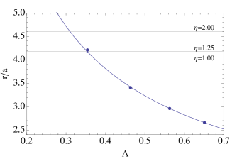
Figure 1: Smearing radius for $m_{\pi}=315\mathop{\hbox{MeV}}$ and lattice spacing $a\approx 0.121\mathop{\hbox{fm}}$. The radius is evaluated on a $16^{3}\times 32$ ensembles for $N_{v}=25$, 50, 75, and 100 and the line represents a power law fit. The horizontal lines indicate the smearing radius corresponding to $N_{v}=100$ on ensembles $\mathcal{E}_{1}$, $\mathcal{E}_{2}$, and $\mathcal{E}_{3}$.

Before we conclude we want to make a couple of points about LapH smearing. One benefit of this method is that we can separate the calculation of the smeared quark propagator $\tilde{M}^{-1}$ from computing the correlation functions. This is very important when using a large variational basis, especially since it allows to add other interpolating fields to the basis without having to redo the inversions. Another point that we want to stress is that the smearing employed here does not represent an approximation. The smeared interpolating fields have the right symmetry properties even when the number of Laplacean eigenvectors $N_{v}$ is very small. If the number is too small the overlap with the physical states is poor and the signal-to-noise ratio will be bad. Finally, even though the number of inversions is much smaller than the total number required for the all-to-all propagator, we still need to compute $4N_{v}\times N_{t}$ inversions for each configuration: 19,200 and $25,600$ inversions per configuration for the $m_{\pi}=315\mathop{\hbox{MeV}}$ and $m_{\pi}=226\mathop{\hbox{MeV}}$ ensembles, respectively. This calculation was done using a GPU implementation of a BiCGstab inverter Alexandru et al. (2012).

II.4 Fitting method

To extract the mass and width of the resonance we need to fit the phase-shift data using a phase-shift parametrization in the resonance region. For the $\rho$-resonance a Breit-Wigner parametrization

$$\tan\delta(E)=\frac{E\,\Gamma(E)}{m_{\rho}^{2}-E^{2}}\quad\text{with}\quad\Gamma(E)=\frac{g_{\rho\pi\pi}^{2}}{6\pi}\frac{p^{3}}{E^{2}},$$ (33)

describes the phase shift well close to the resonance. For a given box geometry, this parametrization can be used to determine the eigenvalues of the Hamiltonian using Lüscher’s formula for $A_{2}^{-}$ irrep in Eq. 4.

ensemble	$N_{t}\times N_{x,y}^{2}\times N_{z}$	$\eta$	$a[\mathop{\hbox{fm}}]$	$N_{\text{cfg}}$	$N_{v}$	$am_{\pi}$	$am_{K}$	$am_{N}$	$am^{pcac}_{u/d}$	$af_{\pi}$	$am^{pcac}_{s}$	$af_{K}$
$\mathcal{E}_{1}$	$48\times 24^{2}\times 24$	$1.0$	$0.1210(2)(24)$	$300$	$100$	$0.1934(5)$	$0.3235(6)$	$0.644(6)$	$0.01237(9)$	$0.0648(8)$	$0.03566(6)$	$0.1015(2)$
$\mathcal{E}_{2}$	$48\times 24^{2}\times 30$	$1.25$	$-$	$-$	$-$	$-$	$-$	$-$	$-$	$-$	$-$	$-$
$\mathcal{E}_{3}$	$48\times 24^{2}\times 48$	$2.0$	$-$	$-$	$-$	$-$	$-$	$-$	$-$	$-$	$-$	$-$
$\mathcal{E}_{4}$	$64\times 24^{2}\times 24$	$1.0$	$0.1215(3)(24)$	$400$	$100$	$0.1390(5)$	$0.3124(8)$	$0.62(1)$	$0.00617(9)$	$0.060(1)$	$0.03358(6)$	$0.0980(2)$
$\mathcal{E}_{5}$	$64\times 24^{2}\times 28$	$1.17$	$-$	$-$	$-$	$-$	$-$	$-$	$-$	$-$	$-$	$-$
$\mathcal{E}_{6}$	$64\times 24^{2}\times 32$	$1.33$	$-$	$-$	$-$	$-$	$-$	$-$	$-$	$-$	$-$	$-$

Table 3: The parameters for the ensembles used in this study. The lattice spacing $a$ for each ensemble is listed as well as the number of gauge configurations $N_{\text{cfg}}$ and the number of eigenvectors used for LapH smearing. $am_{N}$, $af_{\pi}$, and $af_{K}$ represent the nucleon mass, pion decay constant and kaon decay constant in lattice units. The two errors for the lattice spacing are stochastic, from the $w_{0}/a$ determination, and a systematic one estimated to be 2%.

The energies $E_{k}$ satisfying both equations Eq. 33 and Eq. 4 are the expected eigenvalues of the Hamiltonian on periodic boxes with geometry $L^{2}\times\eta L$. These solutions are functions of the geometry of the box $\eta$ and the parameters of the Breit-Wigner curve and we will denote them with $E_{k}(m_{\rho},g_{\rho\pi\pi};\eta)$. To determine the fit parameters we minimize the chi-square function

$$\chi^{2}(m_{\rho},g_{\rho\pi\pi})=\sum_{e}\delta_{e}^{T}C_{e}^{-1}\delta_{e},$$ (34)

where the sum runs over the statistically independent ensembles with different elongations and the residue vector is given by

$$(\delta_{e})_{k}=E_{k}(m_{\rho},g_{\rho\pi\pi};\eta_{e})-E^{(e)}_{k}\,.$$ (35)

Above we denote with $E^{(e)}_{k}$ the $k^{\text{th}}$ energy extracted from ensemble $e$ and with $C_{e}$ the covariance matrix for these energies. Note that the residue vector includes the residues for both zero-momentum states and boosted-states and thus it has between 6 and 8 entries depending on the ensemble considered. The values for $E^{(e)}_{k}$ and covariance matrix $C_{e}$ are given in Appendinx C. The energies are extracted using individual correlated fits and the covariance matrices are estimated using a jackknife analysis.

III Results

In this section we present the results for the energies and phase-shifts extracted from the ensembles used in this study and discuss some of the salient issues. We have generated configurations using Lüscher-Weiss gauge action Lüscher and Weisz (1985); Alford et al. (1995) and nHYP-smeared clover fermions Hasenfratz et al. (2007) with two mass-degenerate quark flavors ($N_{f}=2$). For each mass we generated three sets of ensembles with different elongations. The elongations were chosen to ensure that the energy spectrum for the zero-momentum states in the $A_{2}^{-}$ channel overlaps well with the $\rho$-resonance region, following the procedure described in a previous study Pelissier and Alexandru (2013).

The parameters for these ensembles are listed in Table 3. A couple of comments regarding the parameters listed in the table. The lattice spacing was determined using an observable based on the Wilson flow Lüscher (2010): the $w_{0}$ parameter Borsanyi et al. (2012). This quantity can be determined with very little stochastic error from a handful of configurations. We used 150 configurations from ensembles ${\cal E}_{1}$ and ${\cal E}_{4}$ and computed $w_{0}/a=1.3888(24)$ and $w_{0}/a=1.4157(37)$ respectively. These measurements were used to fix the lattice spacing using the conversion factors determined in Bruno and Sommer (2014): we computed the dimensionless quantity $y=m_{\pi}^{2}t_{0}$, determined $w_{0}(y)/w_{0}(y=0)$ from Fig. 4 in the above reference, and then converted to physical units using $w_{0}(y=0)=0.1776(13)\mathop{\hbox{fm}}$. This value of $w_{0}$ was determined from a set of $N_{f}=2$ simulations where $f_{K}$ was used to set the scale Fritzsch et al. (2012). The scale determined this way differs from the scale we used in our previous study Pelissier and Alexandru (2013) by 3.5%, but we attribute this shift to the fact that the value of the Sommer parameter Sommer (1994) is difficult to define unambiguously on configurations with light quarks. The value we used in our previous study was $r_{0}=0.5\mathop{\hbox{fm}}$, but recent determinations of $r_{0}$ from global fits of the hadronic spectrum favor smaller values Yang et al. (2014); Aoki et al. (2011b) and produce values in agreement with the scale determined based on $w_{0}$. We decided to adopt the scale determined by $w_{0}$ because the method is very straightforward and it has small stochastic errors. Note that at fixed lattice spacing in the presence of lattice artifacts, the lattice spacing determination introduces a systematic error. We estimate that our systematic error associated with the lattice spacing is at the level of 2%. To confirm the correctness of the lattice spacing we looked at the nucleon mass, pion and kaon decays constants. We computed the nucleon mass $m_{N}$ and extrapolated to the physical point using an empirically motivated fit form Walker-Loud (2008). The extrapolated values agree at the level of 2%, but this may be fortuitous since the error bars of the extrapolation were at the level of 4%. In any case this error level is in line with the expectation from other studies that used HEX-smeared fermions at similar lattice spacing Durr et al. (2011), where the hadronic spectrum was found to be shifted by about 2% relative to the continuum. The values of $f_{\pi}$ and $f_{K}$ were determined using the procedure outlined in Fritzsch et al. (2012). For the masses used in our study our values for $f_{K}$ differs by less than 1% from the values determined there at much smaller lattice spacing.

For each ensemble we extract the lowest three or four levels in the $A_{2}^{-}$ channel, since these levels correspond roughly to the elastic region where the center-of-mass energy is below $4m_{\pi}$. To extract the energies we compute the correlation matrix $C(t)$, solve the eigenvalue problem in Eq. 14, and fit the extracted eigenvalues to an exponential ansatz. In Fig. 2 we show the effective mass computed from the three lowest eigenvalues on the ${\cal E}_{1}$ ensemble. Note that the effective mass does not flatten out until later times. To extract the energy we fit a double exponential function constrained to pass through $1$ at $t=t_{0}$: $f_{1}(t)=Ae^{-E(t-t_{0})}+(1-A)e^{-E^{\prime}(t-t_{0})}$. For the lowest $\bm{P}=0$ state on ensemble ${\cal E}_{3}$ this fit form does not work, due to wrap-around effects in the time direction Prelovsek and Mohler (2009); Dudek et al. (2012). We added a constant term to the fit form to accommodate this effect: $f_{2}(t)=Ae^{-E(t-t_{0})}+(1-A-C)e^{-E^{\prime}(t-t_{0})}+C$. We used this fit form with the other zero-momentum states in all the ensembles, but the constant term produced by minimizing $\chi^{2}$ was compatible with zero. For the moving states, the wrap-around effect leads to a small, slowly decaying term with a rate controlled by the mass difference between the moving pion and the pion at rest $\delta E=\sqrt{m_{\pi}^{2}+(2\pi/L)^{2}}-m_{\pi}$ Dudek et al. (2012). For the states where this contribution was significant, we used the following fit form $f_{3}(t)=Ae^{-E(t-t_{0})}+(1-A-C)e^{-E^{\prime}(t-t_{0})}+Ce^{-\delta E(t-t_{0})}$. The fitting details including the choice of $t_{0}$, fitting range, fit form, energy extracted, and quality of the fit are tabulated in Table 6 in the Appendix.

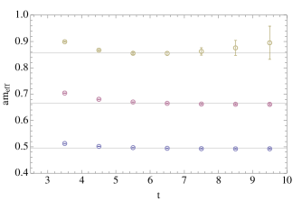
Figure 2: The effective mass for the lowest three energy levels of ${\cal E}_{1}$ ensemble. The dashed line represent the $4m_{\pi}$ threshold. Contamination from higher energy levels is present in the early time slices, therefore we used a double exponential to extract the energy. The horizontal lines indicate the results of the fit.

We discuss now the choice of the interpolator fields and in particular we address the question whether our interpolating field basis overlaps well with the lowest three energy states in the $A_{2}^{-}$ channel. To this end, we compare the energy spectrum extracted using different subsets of the interpolating fields basis. To simplify the discussion we focus first on the ${\cal E}_{1}$ ensemble. The energy spectrum extracted from different interpolating fields basis combinations is plotted in Fig. 3. In the first panel, we include only $q\bar{q}$ operators. While the ground state seems to be well approximated, the $q\bar{q}$ operators have little overlap with the first and second excited states which indicates that they are multi-hadron states. In the second column, we use the $\pi\pi_{100}$ operator together with various combinations of $q\bar{q}$ operators. The ground state and first excited state are well reproduced, even when using only one $q\bar{q}$ interpolator. However, the second excited state has large error-bars even if we add three other $q\bar{q}$ operators, which indicates that it has a large multi-hadron component. In the third panel, we use two multi-hadron interpolators: $\pi\pi_{100}$ and $\pi\pi_{011}$. Once one $q\bar{q}$ operator is added to the basis, all three lowest energy states are well determined with small errorbars. Adding more $q\bar{q}$ operators to the basis does not improve the extraction and we conclude that these lowest three states are well captured by our set of interpolators.

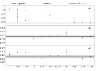
Figure 3: Energy spectrum for ensemble ${\cal E}_{1}$ with different interpolator basis combinations. The horizontal axis labels different interpolator choice: $\mathcal{O}_{1-4}$ are the $q\bar{q}$ interpolating fields, $\mathcal{O}_{5}$ is $\pi\pi_{100}$ and $\mathcal{O}_{6}$ is $\pi\pi_{011}$. The vertical axis represents the energy for the three lowest levels. Note that we use different scales for each level. The three horizontal band shows the energy values extracted from $6\times 6$ correlation matrix. The first panel only includes the $q\bar{q}$ operators. Second panel includes $\pi\pi_{100}$ and various $q\bar{q}$ operators. The third panel has $\pi\pi_{100},\pi\pi_{011}$ with various $q\bar{q}$ operators.

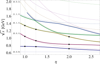
Figure 4: Energy spectrum with different elongated factor from unitary chiral perturbation theory in the rest frame $\mathbf{P}=(0,0,0)$ (solid lines). The error bars of eigenvalues are smaller than the symbol size (black circles). $\eta$ labels the elongated factor, in particular $\eta=1.0,1.25,2.0$ are the ensembles we used for $m_{\pi}\approx 315\mathop{\hbox{MeV}}$. Here, the $\eta=1$ values are fitted and then eigenvalues for $\eta=1.25$ and $\eta=2$ are predicted. The dashed lines represent the energy of non-interacting pion states with various momentum for two pions.

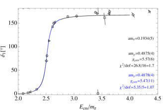
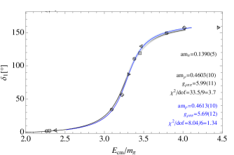
Figure 5: Phase shifts as a function of the center of mass energy. The errorbars are slanted along the direction of the Lüscher curves. On the left we have the $m_{\pi}=315\mathop{\hbox{MeV}}$ data and on the right the $m_{\pi}=226\mathop{\hbox{MeV}}$ data. The triangles, squares, and hexagons correspond to data extracted from ${\cal E}_{1}$, ${\cal E}_{2}$, ${\cal E}_{3}$ (left) and ${\cal E}_{4}$, ${\cal E}_{5}$, ${\cal E}_{6}$ (right) respectively. The black curve, error-bands, and fit parameters correspond to Breit-Wigner fit to all data points in the elastic region, $E_{\text{cm}}<4m_{\pi}$. Blue color indicates the fit to the data in $m_{\rho}\pm 2\Gamma_{\rho}$ region. The U$\chi$PT fits are very close to the blue Breit-Wigner curves.

To confirm the conclusion above, we fit a model based on Unitary Chiral Perturbation theory (see Appendix B) to the energy levels extracted from ensemble ${\cal E}_{1}$ and use it to predict the energy levels for different box elongations. The expected energy levels are plotted in Fig. 4 as a function of the elongation. In the graph we also indicate the expected energy levels for two-pion states in the absence of interactions. We see that for elongation $\eta=1$ which corresponds to ensemble ${\cal E}_{1}$ the ground state is not in the vicinity of any two-pion state and thus it is mainly a $q\bar{q}$ state, whereas the first two excited states are close to non-interacting two-pion states, which indicates that they have large two-hadron components. That is the reason why the multi-hadron operators $\pi\pi_{001}$ and $\pi\pi_{011}$ are required to extract these states reliably. For ${\cal E}_{1}$ and ${\cal E}_{2}$ these multi-hadron operators are sufficient. However, for $\eta=2.0$, the second excited state is no longer near the non-interacting pions moving with back-to-back momentum $\bm{p}=(0,1,1)$, because the state with back-to-back momentum $\bm{p}=(0,0,2)$ has lower energy for this elongation. Note that this level crossing is kinematical in nature rather than due to a resonance. This is a peculiar feature of our geometry due to the fact that the ordering of levels with different transverse momenta changes when going from small elongations to large ones. Thus, in order to extract the second excited state reliably on ${\cal E}_{3}$ and ${\cal E}_{6}$ we need to add the $\pi\pi_{002}$ interpolating field to our basis. For these ensembles we use a $7\times 7$ correlation matrix and extract four energy levels since the third excited state is very close the the second excited state and below the $4m_{\pi}$ threshold. As a result, we will have more data points to fit for the phase shift pattern in next section. The number of energy levels we extracted for each ensemble is listed in Table 6 in Appendix C.

IV Resonance Parameters

We extract the resonance parameters by fitting the phase-shift data, or equivalently the energy levels, using two fitting forms: a simple Breit-Wigner form and a model based on Unitarized Chiral Pertubation Theory (U$\chi$PT). Note that when fitting the phase shift data, the correlation between $E_{\rm cm}$ and $\delta(E_{\rm cm})$ has to be taken into account. The Breit-Wigner form is used in most lattice studies of the $\rho$-resonance since it fits the phase-shift well. This also offers a straightforward way to compare our results with the ones from other studies. The U$\chi$PT model provides an alternative parametrization which also captures well the phase-shift behavior in the $\rho$-resonance region. Its main advantage, and the reason we use it in our study, is that it can be used to fit the data sets at different quark masses simultaneously, and it offers a reasonable way to extrapolate our results to the physical point.

The Breit-Wigner parametrization is described in Eq. 33. In Fig. 5 we show our phase-shifts and the fitted curves. Note that if we try to fit the entire elastic region, $E_{\text{cm}}<4m_{\pi}$, the quality of the fit, as indicated by $\chi^{2}$ per degree of freedom, is not very good. While the curve passes close to our points, our energy level determination is very precise and the Breit-Wigner form is not describing the entire energy range accurately. This is not a serious problem since the Breit-Wigner form is only expected to describe the data well near the resonance. Ideally, we would restrict the fit only to a narrow region around the resonance, but the number of data points included in our fit is also reduced and the fit is poorly constrained. As a compromise we decided to fit the data points that fall in the range $E_{\text{cm}}\in[m_{\rho}-2\Gamma_{\rho},m_{\rho}+2\Gamma_{\rho}]$. The fit quality is improved and we will use the results of the narrower fits in the following discussion. For the heavier pion mass the results in lattice units are

$$am_{\pi}=0.1934(5),\,am_{\rho}=0.4878(4),\,g_{\rho\pi\pi}=5.47(11)$$ (36)

and in physical units

$$\begin{split}&m_{\pi}=315.4(0.8)(6.3)\mathop{\hbox{MeV}}\,,\quad m_{\rho}=795.5(0.7)(16)\mathop{\hbox{MeV}}\,,\\ &\Gamma_{\rho}=35.7(1.4)(0.7)\mathop{\hbox{MeV}}\,,\quad\Gamma^{\prime}_{\rho}=124.4(5)(2.5)\mathop{\hbox{MeV}}\,,\end{split}$$ (37)

where $\Gamma_{\rho}$ is the width at the current pion mass and $\Gamma^{\prime}_{\rho}$ is the width extrapolated to the physical point. The widths are evaluated using Eq. 33 with $\Gamma_{\rho}=\Gamma_{BW}(m_{\rho},m_{\pi})$ and $\Gamma^{\prime}_{\rho}=\Gamma_{BW}(m_{\rho}^{\text{phys}},m_{\pi}^{\text{phys}})$. The first error is the stochastic error and the second one is the systematic error due to the lattice spacing determination. For the lighter pion mass we have

$$am_{\pi}=0.1390(5)\,,am_{\rho}=0.4613(10)\,,g_{\rho\pi\pi}=5.69(12)\,,$$ (38)

and in physical units

$$\begin{split}&m_{\pi}=225.7(0.8)(4.5)\mathop{\hbox{MeV}}\,,\quad m_{\rho}=749.2(1.6)(15)\mathop{\hbox{MeV}}\,,\\ &\Gamma_{\rho}=81.7(3.3)(1.6)\mathop{\hbox{MeV}}\,,\quad\Gamma^{\prime}_{\rho}=134.4(5)(2.7)\mathop{\hbox{MeV}}\,.\end{split}$$ (39)

We note that the Breit-Wigner fit parameters depend mildly on the range of the fit. The mass of the resonance is very well determined, with stochastic errors of the order of few parts per thousand, and it is insensitive to the fit range. This is because the place where the phase-shift passes through $\pi/2$ is well constrained by the lattice data. The coupling $g_{\rho\pi\pi}$ is only constrained at the level of two percent and it is more sensitive to the fit range, showing a clear drift towards lower values as we narrow the fitting range.

If we are interested in capturing the phase-shift behavior in the entire energy range available, we could use slight variations of the Breit-Wigner parametrization. Indeed we found that the quality of the fit in the full elastic region is improved when adding barrier terms von Hippel and Quigg (1972), especially on the larger pion mass ensemble. However, such fitting forms change the way the resonance mass and width are defined making it harder to compare our results directly with other determinations and we will not discuss these results here. We include all the relevant data for the extracted energies and their correlation matrix in Appendix C and invite the interested reader to use it to fit any desired parametrization.

For the Breit-Wigner fit we found that the quality of the fit changes significantly as we vary the pion mass within its error bounds. If the Breit-Wigner fit was known to be the exact description of the phase shift in the elastic region, we could in principle use the pion mass as a fitting parameter in this fit to further constrain its value. Since this is not the case, we did not attempt to do this here.

We turn now to the discussion of the fit using the U$\chi$PT model. A description is provided in Appendix B. An important feature is that this model can be used to fit the phase-shift for both quark masses simultaneously. This allows us to extrapolate the results to the physical point and also to assess the corrections due to the missing strange quark mass in our calculation. When considering only the $\pi$-$\pi$ channel, the model requires as input the pion mass, the pion decay constant and two low-energy constants, $\hat{l}_{1,2}$. The pion mass and decay constants used are the ones in Table 3. Note that the model can take directly dimensionless input–$am_{\pi}$, $af_{\pi}$ and the energies $aE$—so the systematic errors associated with the lattice spacings play no role in the extraction of dimensionless parameters $\hat{l}_{1,2}$. The error-bars that appear in the tables below reflect just the stochastic error.

$m_{\pi}\,[\mathop{\hbox{MeV}}]$	$\hat{l}_{1}\times 10^{3}$	$\hat{l}_{2}\times 10^{3}$	$m_{\rho}[\mathop{\hbox{MeV}}]$	$\Gamma_{\rho}[\mathop{\hbox{MeV}}]$	$\chi^{2}/\text{dof}$
315	1.5(5)	-3.7(2)	796(1)	35(1)	1
138			704(5)	110(3)
226	2(1)	-3.5(2)	748(1)	77(1)	1.53
138			719(4)	120(3)
combined	2.26(14)	-3.44(3)			1.26
138			720(1)	120.8(8)

Table 4: U$\chi$PT fits in the $m_{\rho}\pm 2\Gamma_{\rho}$ region and extrapolations to the physical point. The errors quoted are statistical. The upper two entries show the cases of heavy and light pion mass, both individually extrapolated to the physical point. The third entry shows the combined fit of both masses and its extrapolation.

In Table 4 we show the results of fitting the U$\chi$PT model. The model is similar to the Breit-Wigner parametrization: it captures the broad features of the phase-shift in the elastic region but the quality of the fit is not good when trying to fit all energy range. We restrict the fit range to $m_{\rho}\pm 2\Gamma_{\rho}$, as we did for Breit-Wigner parametrization. In this range the quality of the fit is reasonable. The resonance mass is determined from the center-of-mass energy that corresponds to a $90^{\circ}$ phase-shift. The width corresponds to the imaginary value of the resonance pole in the complex plane. While these parameter definitions are not the same as the ones determined from the Breit-Wigner fit, the results are consistent as can be seen from the table.

Fitting each quark mass separately produces consistent values for $\hat{l}_{1,2}$ which indicates that the phase-shift dependence on the quark mass is well captured by this model. Since the model is consistent for both quark masses we can do a combined fit which allows us to pin down $\hat{l}_{1,2}$ with even better precision. As can be seen from the table the combined fit quality is similar to the individual ones. We will use these parameters in the subsequent discussion.

Moreover, we can try to estimate the effects due to the strange quark using the U$\chi$PT model by turning on the coupling to the K$\bar{\rm K}$ channel. We fix the $\pi\pi\to K\bar{K}$ and $K\bar{K}\to K\bar{K}$ transitions from a fit to the physical data, while keeping $\hat{l}_{1,2}$ for the $\pi\pi$ transition at the values we got from fitting our data. The pion decay constant is adjusted to mach the values in Table 3. We report these estimates in Table 5. More details about the U$\chi$PT fit are included in Appending B.

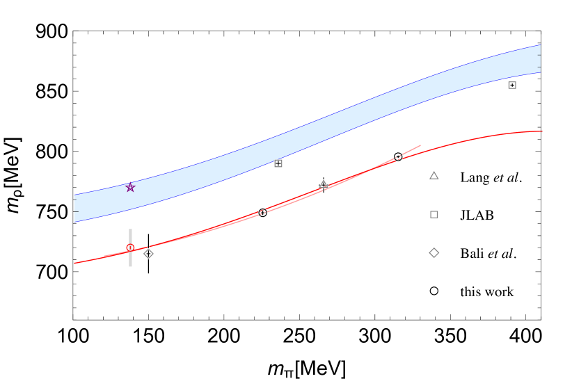
Figure 6: Resonance mass extrapolation to the physical point. The red curve corresponds to an extrapolation based on the U$\chi$PT model. The light-red curve corresponds to a simple $m_{\rho}=(m_{\rho})_{0}+\text{const}\times m_{\pi}^{2}$ fit Bruns and Meissner (2005). The blue band corresponds to an $N_{f}=2+1$ estimate based on the U$\chi$PT model (see text). The other lattice data-points are taken from Lang et al Lang et al. (2011), JLab group studies Dudek et al. (2013); Wilson et al. (2015), and Bali et al Bali et al. (2016). The star corresponds to the physical result. The error-bars shown with solid lines are stochastic. For the extrapolation the gray, thick error-bar indicates the systematic error associated with the lattice spacing determination.

In Fig. 6 we plot our results for the resonance mass together with the U$\chi$PT extrapolation, in comparison with results from other lattice groups. It is clear that the extrapolation to the physical point in SU(2) is significantly below the experimental value, missing it by about $50\mathop{\hbox{MeV}}$ which is about 8% of the resonance mass. The stochastic error for the extrapolated result is tiny compared with the shift. The systematic error due to the lattice spacing determination is larger, but even this cannot account for the discrepancy. The other possible sources of systematic errors are finite lattice spacing contributions, finite volume corrections, quark mass extrapolation error, and systematics associated with the missing K$\overline{\rm K}$ channel. The lattice artifacts errors are included in our estimate for the systematic error associated with the lattice spacing determination. To gauge the effect of the lattice volume corrections we compare our results with the ones from a study by Lang et al Lang et al. (2011). This study was carried out on boxes of volume $(2\mathop{\hbox{fm}})^{3}$, whereas our study uses boxes of about $(3\mathop{\hbox{fm}})^{3}$. We see in Fig. 6 that the results agree and we conclude that the finite volume corrections cannot account for the discrepancy either. The errors associated with the quark mass extrapolation are also expected to be small: in Fig. 6 we show the results of the extrapolation using a simple polynomial extrapolation which at leading order depends on $m_{\pi}^{2}$ Bruns and Meissner (2005). The extrapolation agrees well with the prediction of U$\chi$PT in SU(2). Moreover, a recent calculation by Bali et al Bali et al. (2016) close to the physical quark mass is also consistent with our extrapolation.

$m_{\pi}\,[\mathop{\hbox{MeV}}]$	$m_{\rho}[\mathop{\hbox{MeV}}]$	$\Gamma_{\rho}[\mathop{\hbox{MeV}}]$	$\hat{m}_{\rho}[\mathop{\hbox{MeV}}]$	$\hat{\Gamma}_{\rho}[\mathop{\hbox{MeV}}]$
315	795.2(7)	36.5(2)	846(0.3)(10)	54(0.1)(3)
226	747.6(6)	77.5(5)	793(0.4)(10)	99(0.3)(3)
138	720(1)	120.8(8)	766(0.7)(11)	150(0.4)(5)

Table 5: U$\chi$PT results for $N_{f}=2$, $m_{\rho}$ and $\Gamma_{\rho}$, and $N_{f}=2+1$ estimates, $\hat{m}_{\rho}$ and $\hat{\Gamma}_{\rho}$. The parameters $\hat{l}_{1,2}$ are taken from the combined fit and the K$\overline{\rm K}$ channel parameters are taken from fits to experimental data. The first set of errors quoted are statistical; for $\hat{m}_{\rho}$ and $\hat{\Gamma}_{\rho}$ we also quote a set of systematic errors associated with model dependence (see Appendix B for details).

The likely reason for the discrepancy between the extrapolation and the physical result is the fact that the strange quark flavor is not included in our calculation. We note first that the results for U$\chi$PT  in SU(2) agree very well with the results of in the other $N_{f}=2$ studies by Lang and Bali. The results when the strange quark is included are also shown in Fig. 6 (blue band indicating estimated model uncertainties as discussed in Appendix B). Note that the estimated shift is surprisingly large and it reduces the discrepancy substantially. The estimated resonance mass curve agrees quite well with a $N_{f}=2+1$ lattice calculations reported by the Jlab group Dudek et al. (2013); Wilson et al. (2015). While these estimates are likely affected by systematic errors, we feel that they are accurate enough to indicate that the discrepancy is mostly generated by the absence of the strange quark in our calculation. We note that the magnitude of the shift in the resonance mass due to the inclusion of the K$\bar{\rm K}$ channel is surprisingly large. The present work stresses the importance of taking into account $\pi\pi-K\bar{K}$ loops, which is the strength of the prediction of the U$\chi$PT model. We will discuss this point in detail in an upcoming publication Hu et al. (2016).

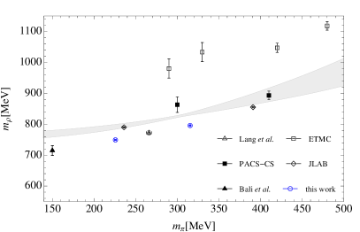
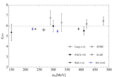
Figure 7: Comparison of different lattice calculation for the $\rho$ resonance mass (left) and width parameter $g_{\rho\pi\pi}$ (right). The errors included here are only stochastic. The results labeled ETMC are taken from Feng et al. (2011) and PACS from Aoki et al. (2011a). The band in the left plot indicates a $N_{f}=2+1$ expectation from U$\chi$PT model constrained by some older lattice QCD data and some other physical input Pelaez and Rios (2010). The dotted line in the right plot indicates the $g_{\rho\pi\pi}$ that corresponds to the physical rho width Olive et al. (2014).

V Conclusions

We presented a high-precision calculation of the phase-shift in the $I=1$, $J=1$ channel for $\pi\pi$ scattering. To scan the resonance region we elongated the lattice in only one direction, which makes the generation of configuration less expensive. We used two sets of ensembles, each with three different elongations, for two different quark masses. To compute the phase-shift we extracted the energies in the $A_{2}^{-}$ channel both for states at rest and for states with one unit of momentum in the elongated direction. The required two-, three-, and four-point correlation functions were computed using the LapH method. Elongated boxes have a different symmetry than cubic ones and different Lüscher formulas are required: for the zero-momentum case they were worked out in Feng et al. (2004); Li and Liu (2004) and in this paper we worked out the required one for states boosted along the elongated direction.

The phase-shifts are broadly described by a Breit-Wigner parametrization, as expected. However, our calculation is precise enough to show that more sophisticated models are required to describe the variation of the phase-shift in the entire elastic region. It is hoped that our results can be used to validate these models and to constrain their parameters.

The resonance mass and $g_{\rho\pi\pi}$ coupling are extracted from fitting a Breit-Wigner parametrization in the energy region $m_{\rho}\pm 2\Gamma_{\rho}$. In Fig. 7 we compare our results with other lattice determinations. Other than the ETMC study, the lattice data seems to be split in two groups: $N_{f}=2+1$ results (PACS Aoki et al. (2011a) and Jlab Dudek et al. (2013); Wilson et al. (2015)) which are in agreement with $N_{f}=2+1$ expectations from U$\chi$PT Pelaez and Rios (2010), and $N_{f}=2$ lattice data (Lang et al Lang et al. (2011), Bali et al Bali et al. (2016), and this work) that agrees with a $N_{f}=2$ U$\chi$PT model fit to our data.

For the resonance mass, we performed an extrapolation to the physical mass using a U$\chi$PT model, which we found can describe well the phase-shift data at both quark masses using the same parameters. The extrapolation results are consistent with extrapolations based on other models Bruns and Meissner (2005) and other $N_{f}=2$ lattice calculations, as discussed before. The extrapolated results differ significantly from the physical one and we argue that this is due to the absence of the strange quark in our calculation.

For the quark masses used in this study, we did not find evidence of significant finite volume effects. However, as we lower the pion mass, larger volumes would most likely be required. The original LapH method might turn out to be too expensive to apply directly, but a stochastic variant was already developed and showed to work well Bulava et al. (2016). Note that we did not include these data points in Fig. 7 because this study is using the same ensemble as the Jlab group study Wilson et al. (2015) and their results are compatible with the ones computed by the Jlab group, albeit with slightly larger errorbars.

Turning to the future, as far as phase-shifts in the $\rho$ resonance channel are concerned, we seem to have moved beyond proof-of-principle calculations and toward precision determinations. We anticipate that in the near future precise calculations at the physical point might be possible that will give us access directly to phase-shifts to be compared to values extracted from physical data. For example, it would be interesting to see whether phaseshifts close to threshold match chiral perturbation theory expectations, which at leading order are controlled solely by $m_{\pi}$ and $f_{\pi}$. The phaseshifts calculated in this study do not agree well with this prediction even for the data points closest to the threshold. Note that even the experimental determined phases also do not agree with the lowest order chiral perturbation predictions.

Other channels are also of interest, for example the $I=0$ channel where the broad sigma resonance is expected to appear, $\pi$-K scattering in the $K^{*}$ channels, baryon-meson scattering, etc. We plan to investigate some of these channels in the near future.

Appendix A Zeta function

To compute the phase shift in Eq. 4 we need to numerically evaluate the zeta function. For the zero momentum case the relevant formulas for elongated boxes were derived in Li and Liu (2004); Feng et al. (2004). In the following we will show how to extend this to the non-zero momentum states, when the boost is parallel with the elongated direction of the box. We discuss first the evaluation of the zeta function for cubic boxes and then extend it to accommodate elongated boxes. For a boosted state with momentum $\bm{P}=\bm{d}2\pi/L$, the zeta function in a cubic box is

$$\mathcal{Z}_{lm}^{\bm{d}}(s;q,\gamma)=\sum_{\bm{n}\in P_{\bm{d}}(\gamma,\eta)}\frac{\mathcal{Y}_{lm}(\bm{n})}{(\bm{n}^{2}-q^{2})^{s}},$$ (40)

with

$$P_{d}(\gamma)=\left\{\bm{n}\in\mathds{R}^{3}\Big{|}\bm{n}=\hat{\gamma}^{-1}\left({\bm{m}}+\frac{\bm{d}}{2}\right),\bm{m}\in{\mathds{Z}}^{3}\right\}.$$ (41)

The series above is only convergent when $\mathop{\hbox{Re}}s>l+3/2$ but the zeta function needs to be evaluated at $s=1$. The function defined by the series above can be analytically continued in the region $\mathop{\hbox{Re}}s>1/4$. The analytic continuation is done following Lüscher Lüscher (1991) and Rummukainen Rummukainen and Gottlieb (1995) using the heat kernel expansion

$$\begin{split}\mathcal{K}(t,\bm{x})&=\frac{1}{(2\pi)^{3}}\sum_{\bm{n}\in P_{\bm{d}}(\gamma)}e^{i\bm{n}\cdot\bm{x}-t\bm{n}^{2}}\\ &=\frac{\gamma}{(4\pi t)^{\frac{3}{2}}}\sum_{\bm{n}\in P_{\bm{0}}(1/\gamma)}e^{i2\pi(\hat{\gamma}^{-1}\bm{n})\cdot\bm{d}/2}e^{-\frac{1}{4t}(\bm{x}+2\pi\bm{n})^{2}}\,.\end{split}$$ (42)

This relation is obtained using Poisson’s summation formula

$$\sum_{n\in Z^{3}}f(\bm{n})=\sum_{k\in Z^{3}}\int^{\infty}_{-\infty}f(\bm{x})e^{i2\pi\bm{k}\cdot\bm{x}}d^{3}x.$$ (43)

The spherical projected kernel $\mathcal{K}_{lm}$ is defined as $\mathcal{K}_{lm}=\mathcal{Y}_{lm}(-i\nabla)\mathcal{K}$ which can be written as

$$\begin{split}&\mathcal{K}_{lm}^{\bm{d}}(t,\bm{x})=(2\pi)^{-3/2}\sum_{\bm{n}\in P_{\bm{d}}}\mathcal{Y}_{lm}(\bm{n})e^{(i\bm{n}\cdot\bm{x}-t\bm{n}^{2})}\\ &=\frac{\gamma}{(4\pi t)^{3/2}}\frac{i^{l}}{(2t)^{l}}\sum_{\bm{n}\in Z^{3}}(-1)^{\bm{d}\cdot\bm{n}}\mathcal{Y}_{lm}(\bm{x}+2\pi\hat{\gamma}\bm{n})e^{-\frac{1}{4t}(\bm{x}+2\pi\hat{\gamma}\bm{n})^{2}}\,.\end{split}$$ (44)

Using the truncated kernels $\mathcal{K}_{lm}^{\Lambda}=\mathcal{Y}_{lm}(-i\nabla)\mathcal{K}^{\Lambda}$ with

$$\mathcal{K}^{\Lambda}(t,\bm{x})\equiv\frac{1}{(2\pi)^{3}}\sum_{\bm{n}\in P_{\bm{d}}(\gamma),|\bm{n}|\leq\Lambda}e^{i\bm{n}\cdot\bm{x}-t\bm{n}^{2}}\,,$$ (45)

we define the zeta function by separating the series terms in two groups, a finite set close to the origin that remains in the original form, and the rest that will be evaluated via an kernel integral:

$$\begin{split}&\mathcal{Z}_{lm}^{\bm{d}}(s;q,\gamma)\\ &=\sum_{\begin{subarray}{c}\bm{n}\in P_{\bm{d}}(\gamma)\\ |\bm{n}|<\Lambda\end{subarray}}\frac{\mathcal{Y}_{lm}(\bm{n})}{(\bm{n}^{2}-q^{2})^{s}}+\frac{(2\pi)^{3}}{\Gamma(s)}\left\{\frac{\delta_{l0}\delta_{m0}\gamma}{(4\pi)^{2}(s-3/2)}\right.\\ &+\int^{1}_{0}dtt^{s-1}\left[e^{tq^{2}}\mathcal{K}_{lm}^{\Lambda}(t,\bm{0})-\frac{\delta_{l0}\delta_{m0}\gamma}{(4\pi)^{2}t^{3/2}}\right]\\ &+\left.\int^{\infty}_{1}e^{tq^{2}}\mathcal{K}_{lm}^{\Lambda}(t,\bm{0})\right\}\,.\end{split}$$ (46)

For the integral on the $t\in[1,\infty]$ range, the heat kernel expansion in terms of $\exp(i\bm{n}\cdot\bm{x}-t\bm{n}^{2})$ is used, and on the $t\in[0,1]$ range, the expansion in terms of $\exp[-(\bm{x}+2\pi\bm{n})^{2}/4t]$ is used. In both cases the series converges the slowest around $t=1$: for the $t\in[1,\infty]$ range large $\bm{n}$ terms contribute $\exp(-t(\bm{n}^{2}-q^{2}))$ and on the $t\in[0,1]$ range they contribute $\exp[tq^{2}-(2\pi\bm{n})^{2}/4t]$. It is clear that this series converges quickly for large $\bm{n}$ if we choose $\Lambda>\mathop{\hbox{Re}}q^{2}$. For the $A_{2}^{-}$ irrep we need to evaluate $\mathcal{Z}^{\bm{d}}_{00}$ and $\mathcal{Z}^{\bm{d}}_{20}$. For $\mathcal{Z}_{00}^{\bm{d}}$, we have

$$\begin{split}&\mathcal{Z}^{\bm{d}}_{00}(s;q,\gamma)\\ &=\sum_{\begin{subarray}{c}\bm{n}\in P_{\bm{d}}(\gamma)\\ |\bm{n}|\leq\Lambda\end{subarray}}\frac{\mathcal{Y}_{00}(\bm{n})}{(\bm{n}^{2}-q^{2})^{s}}+\frac{\pi\gamma}{2\Gamma(s)(s-3/2)}\\ &+\gamma\sum_{\bm{n}\in P_{\bm{0}}(1/\gamma)}e^{i2\pi(\hat{\gamma}^{-1}\bm{n})\cdot\bm{d}/2}\mathcal{Y}_{00}(\bm{n})I_{00}(s,q,|\bm{n}|)\\ &-\sum_{\begin{subarray}{c}\bm{n}\in P_{\bm{d}}(\gamma)\\ |\bm{n}|\leq\Lambda\end{subarray}}\mathcal{Y}_{00}(\bm{n})\underline{J}_{00}(s,q,|\bm{n}|)\\ &+\sum_{\begin{subarray}{c}\bm{n}\in P_{\bm{d}}(\gamma)\\ |\bm{n}|>\Lambda\end{subarray}}\mathcal{Y}_{00}(\bm{n})\bar{J}_{00}(s,q,\gamma,|\bm{n}|)\,,\end{split}$$ (47)

where $\mathcal{Y}_{00}(\bm{n})=\frac{1}{\sqrt{4\pi}}$ and the notation used is:

$$\begin{split}I_{00}(s,q,|\bm{n}|)&=\frac{(2\pi)^{3}}{\Gamma(s)}\int_{0}^{1}dtt^{s-1}\frac{(e^{tq^{2}-(2\pi\bm{n})^{2}/4t}-\delta_{|\bm{n}|0})}{(4\pi t)^{3/2}}\,,\\ \underline{J}_{00}(s,q,|\bm{n}|)&=\frac{1}{\Gamma(s)}\int^{1}_{0}dtt^{s-1}e^{tq^{2}}e^{-t\bm{n}^{2}}\,,\\ \bar{J}_{00}(s,q,|\bm{n}|)&=\frac{1}{\Gamma(s)}\int^{\infty}_{1}dtt^{s-1}e^{tq^{2}}e^{-tn^{2}}\\ &=\frac{1}{(\bm{n}^{2}-q^{2})^{s}}-\underline{J}_{00}(s,q,|\bm{n}|)\,.\end{split}$$ (48)

These functions can be expressed in terms of Euler gamma function and exponential integral function

$$\begin{split}\Gamma(s,z)=\int_{z}^{\infty}t^{s-1}e^{-t}dt\,,\quad E_{n}(z)=\int_{1}^{\infty}\frac{e^{-zt}}{t^{n}}dt\,.\end{split}$$ (49)

We have

$$\begin{split}\underline{J}_{00}(s,q,|\bm{n}|)&=\frac{1}{(\bm{n}^{2}-q^{2})^{s}}\left(1-\frac{\Gamma(s,\bm{n}^{2}-q^{2})}{\Gamma(s,0)}\right)\,,\\ \bar{J}_{00}(s,q,|\bm{n}|)&=E_{1-s}(\bm{n}^{2}-q^{2})\ \text{for}\ \mathbf{n}^{2}>q^{2}\,.\end{split}$$ (50)

Therefore, the zeta function can be simplified to

$$\begin{split}\mathcal{Z}_{00}^{\bm{d}}(s;q,\gamma)&=\frac{\pi\gamma}{2\Gamma(s)(s-3/2)}+\sum_{\bm{n}\in P_{\bm{n}}(\gamma)}\mathcal{Y}_{00}(\bm{n})\bar{J}_{00}(s,q,|\bm{n}|)\\ &+\gamma\sum_{\bm{n}\in P_{\bm{0}}(1/\gamma)}e^{i2\pi(\hat{\gamma}^{-1}\bm{n})\cdot\bm{d}/2}\mathcal{Y}_{00}(\bm{n})I_{00}(s,q,|\bm{n}|),\\ \mathcal{Z}_{20}^{\bm{d}}(s;q,\gamma)&=\gamma\sum_{\bm{n}\in P_{\bm{0}}(1/\gamma)}e^{i2\pi(\hat{\gamma}^{-1}\bm{n})\cdot\bm{d}/2}\mathcal{Y}_{20}(\bm{n})I_{20}(s,q,|\bm{n}|)\\ &+\sum_{\bm{n}\in P_{\bm{d}}(r)}\mathcal{Y}_{20}(\bm{n})\bar{J}_{00}(s,q,|\bm{n}|)\,.\end{split}$$ (51)

For the case of interest, $s=1$, the $J_{00}$ and $I_{00}$ integrals are

$$\begin{split}\bar{J}_{00}(1,q,|\bm{n}|)&=\frac{e^{-(\bm{n}^{2}-q^{2})}}{\bm{n}^{2}-q^{2}},\\ I_{00}(1,q,0)&=2\pi^{3/2}[1-e^{q^{2}}-\sqrt{\pi}iq\mathop{\hbox{erf}}(iq)]\,,\\ I_{00}(1,q,|\bm{n}|\not=0)&=\frac{\pi}{|\bm{n}|}Re[e^{2\pi iq|\bm{n}|}(1-\mathop{\hbox{erf}}(iq+\pi|\bm{n}|))]\,.\end{split}$$ (52)

Similarly, for $s=1$, the $I_{20}$ integral can simplify to

$$\begin{split}&I_{20}(1,q,|\bm{n}|)=-\frac{(3+2\bm{n}^{2})e^{q^{2}-(\pi\bm{n})^{2}}}{2|\bm{n}|^{4}\sqrt{\pi}}\\ &+\mathop{\hbox{Re}}\frac{e^{2\pi iq|\bm{n}|}[-3+2\pi q|\bm{n}|(3i+2\pi q|\bm{n}|)][1-\text{erf}(iq+\pi|\bm{n}|)]}{4|\bm{n}|^{5}\pi}\end{split}$$ (53)

where the error function is defined as

$$\mathop{\hbox{erf}}(z)=\frac{2}{\sqrt{\pi}}\int_{0}^{z}e^{-t^{2}}dt\,.$$ (54)

All the relations above work for $\bm{n}^{2}-q^{2}\neq 0$. The series are divergent at the points where $\bm{n}^{2}=q^{2}$. To avoid this trivial divergence these points are removed from the summation, that is

$$\mathcal{Z}_{lm}^{\bm{d}}(s;q,\gamma)=\sum_{\begin{subarray}{c}\bm{n}\in P_{\bm{d}}(\gamma)\\ \bm{n}^{2}\neq q^{2}\end{subarray}}\frac{\mathcal{Y}_{lm}(\bm{n})}{(\bm{n}^{2}-q^{2})^{s}}\,.$$ (55)

This basically amounts to replacing $1/(\bm{n}^{2}-q^{2})$ with $0$ when $\bm{n}^{2}=q^{2}$. In the simplified expressions above this is equivalent to setting

$$\bar{J}_{lm}(s,q,|\bm{n}|)=-\frac{1}{s\Gamma(s)}$$ (56)

when $q^{2}=|\bm{n}|^{2}$. This is because the convergent counterpart $\underline{J}_{lm}(s,q,|\bm{n}|)=1/s\Gamma(s)$ for $s>0$ when $q^{2}=\bm{n}^{2}$ and the sum of $\bar{J}_{lm}$ and $\underline{J}_{lm}$ is $1/(\bm{n}^{2}-q^{2})$ which is replaced with $0$.

For the elongated box case the zeta functions also depend on the elongation factor $\eta$. The only difference is the domain of the summation which becomes

$$P_{\bm{d}}(\gamma,\eta)=\left\{\bm{n}\in\mathds{R}^{3}\Big{|}\bm{n}=\hat{\gamma}^{-1}\hat{\eta}^{-1}(\bm{m}+\frac{\bm{d}}{2}),\bm{m}\in{\mathds{Z}}^{3}\right\}\,,$$ (57)

where $\hat{\gamma}$ and $\hat{\eta}$ are defined in Eq. 9 and Eq. 12. In sum, they can be calculated as

$$\begin{split}\mathcal{Z}_{00}^{\bm{d}}(s;q,\gamma,\eta)&=\mathcal{Z}_{00}^{\bm{d}}(s;q,\gamma\eta)\,,\\ \mathcal{Z}_{20}^{\bm{d}}(s;q,\gamma,\eta)&=\mathcal{Z}_{20}^{\bm{d}}(s;q,\gamma\eta)\,.\end{split}$$ (58)

Appendix B Unitarized chiral perturbation theory model

Chiral Perturbation Theory ($\chi$PT) is successful in describing the meson-meson interaction at low energies Gasser and Leutwyler (1984, 1985). However, the convergence of the amplitude expansion in powers of the meson momenta becomes slow when the energy increases. Moreover, the perturbative expansion fails in the vicinity of resonances, such as $\sigma$ or $\rho$ mesons. To describe the resonant phase shifts and inelasticities extracted from meson-meson scattering, one needs to extend the theory to higher energies. Unitarized Chiral Perturbation Theory (U$\chi$PT) is a nonperturbative method which combines constraints from chiral symmetry and its breaking and (coupled-channel) unitarity. The method of Ref. Oller et al. (1999) uses the ${\cal O}(p^{2})$ and ${\cal O}(p^{4})$ chiral Lagrangians together with a coupled-channel scattering equation which implements unitarity, and is able to describe the meson-meson interaction up to about $1.2\mathop{\hbox{GeV}}$. The resulting amplitudes show poles in the complex plane that can be associated with the known scalar and vector resonances. In the context of the Inverse Amplitud method Truong (1988); Dobado et al. (1990); Dobado and Pelaez (1993, 1997); Nebreda and Pelaez. (2010), the two-meson scattering equation reads Oller et al. (1999)

$$T=[I-VG]^{-1}V$$ (59)

where

$$V=V_{2}[V_{2}-V_{4}]^{-1}V_{2}\,.$$ (60)

In Eq. 59, $G$ is a diagonal matrix whose elements are the two-meson loop functions, evaluated in our case in dimensional regularization in contrast to the cut-off-scheme used in the original model of Ref. Oller et al. (1999):

$$G^{DR}_{ii}(E) =i\,\int\frac{d^{4}q}{(2\pi)^{4}}\,\frac{1}{q^{2}-m_{1}^{2}+i\epsilon}\,\frac{1}{(P-q)^{2}-m_{2}^{2}+i\epsilon}$$ (61)

$$=\frac{1}{16\pi^{2}}\left\{a(\mu)+\ln\frac{m_{1}^{2}}{\mu^{2}}\right.\left.+\frac{m_{2}^{2}-m_{1}^{2}+E^{2}}{2E^{2}}\ln\frac{m_{2}^{2}}{m_{1}^{2}}\right.$$

$$+\frac{p_{i}}{E}\left[\ln(\hskip 5.69046ptE^{2}-(m_{1}^{2}-m_{2}^{2})+2p_{i}E)\right.$$

$$+\ln(\hskip 5.69046ptE^{2}+(m_{1}^{2}-m_{2}^{2})+2p_{i}E)$$

$$-\ln(-E^{2}+(m_{1}^{2}-m_{2}^{2})+2p_{i}E)$$

$$\left.\left.-\ln(-E^{2}-(m_{1}^{2}-m_{2}^{2})+2p_{i}E)\right]\right\},$$

where $p_{i}=\frac{\sqrt{(E^{2}-(m_{1}+m_{2})^{2})(E^{2}-(m_{1}-m_{2})^{2})}}{2E}$ for the channel $i$, $E$ is the center-of-mass energy, and $m_{1,2}$ refers to the masses of the mesons $1,2$ in the $i$ channel. Throughout this study we use $\mu=1$ GeV and a natural value of the subtraction constant $\alpha(\mu)=-1.28$.

For the case of the $\pi-\pi$ interaction with $(I=1;L=1)$, the kernel of Eq. 59, $V(\pi\pi)$, can be expressed as Oller et al. (1999)

$$V(\pi\pi)=\frac{-2\,p^{2}}{3(f_{\pi}^{2}-8\,\hat{l}_{1}m_{\pi}^{2}+4\,\hat{l}_{2}E^{2})}\ ,$$ (62)

where specific combinations of LECs have been introduced, $\hat{l}_{1}\equiv 2\,L_{4}+L_{5}$ and $\hat{l}_{2}\equiv 2\,L_{1}-L_{2}+L_{3}$. Note that these are not identical to the SU(2) CHPT low-energy constants. The one-channel reduction given by Eq. 62, which contains the lowest- and next-to-leading order contributions, constitutes the fit model for the $N_{f}=2$ lattice data of this study.

Coupled channel case ($\pi\pi-K\bar{K}$)

In this section we describe the meson-meson interaction in terms of the partial-wave decomposition of the amplitude and apply it to the case of the $\pi\pi-K\bar{K}$ system with quantum numbers $(L=1;I=1)$. The partial wave decomposition of the scattering amplitude of two spinless mesons with definite isospin $I$ can be written as

$$T_{I}=\sum_{J}(2J+1)T_{IJ}P_{J}(\cos\theta)\,.$$ (63)

where

$$T_{IJ}=\frac{1}{2}\int^{1}_{-1}P_{J}(\cos\,\theta)T_{I}(\theta)\,\,{\rm d}\cos\theta\,.$$ (64)

In the case of two coupled channels, $T_{IJ}$ is a $2\times 2$ matrix whose elements $(T_{IJ})_{ij}$ are related to $S$ matrix elements through the equations (omitting the $I,J$ labels from here on)

$$\begin{split}&(T)_{11}=-\frac{8\pi E}{2ip_{1}}[(S)_{11}-1]\ ,\quad(T)_{22}=-\frac{8\pi E}{2ip_{2}}[(S)_{22}-1]\,,\\ &(T)_{12}=(T)_{21}=-\frac{8\pi E}{2i\sqrt{p_{1}p_{2}}}(S)_{12}\,,\end{split}$$ (65)

with $p_{1}$, $p_{2}$ the center-of-mas momenta of the mesons in channel $1$ ($\pi\pi$) or $2$ ($K\bar{K}$) respectively, that is $p_{i}=\sqrt{(E/2)^{2}-m_{i}^{2}}$. The $S$-matrix can be parametrized as

$$S=\begin{pmatrix}\eta e^{2i\delta_{1}}&i(1-\eta^{2})^{1/2}e^{i(\delta_{1}+\delta_{2})}\\ i(1-\eta^{2})^{1/2}e^{i(\delta_{1}+\delta_{2})}&\eta e^{2i\delta_{2}}\end{pmatrix}\,.$$ (66)

The interaction in the $\pi\pi-K\bar{K}$ system, is evaluated from the ${\cal O}(p^{2})$ and ${\cal O}(p^{4})$ Lagrangians of the $\chi$PT expansion Gasser and Leutwyler (1984, 1985). The potentials, $V_{2}$ and $V_{4}$, projected in $I=1$ and $L=1$ are Oller et al. (1999)

$$V_{2}(E)=-\begin{pmatrix}\frac{2p^{2}_{\pi}}{3f_{\pi}^{2}}&\frac{\sqrt{2}p_{K}p_{\pi}}{3f_{K}f_{\pi}}\\ \frac{\sqrt{2}p_{K}p_{\pi}}{3f_{K}f_{\pi}}&\frac{p_{K}^{2}}{3f_{K}^{2}}\end{pmatrix}$$ (67)

and

$$\begin{split}&V_{4}(E)=-1\times\\ &\begin{pmatrix}\frac{8p_{\pi}^{2}(2\hat{l}_{1}m_{\pi}^{2}-\hat{l}_{2}E^{2})}{3f_{\pi}^{4}}&\frac{8p_{\pi}p_{K}(L_{5}(m_{K}^{2}+m_{\pi}^{2})-L_{3}E^{2})}{3\sqrt{2}f_{\pi}^{2}f_{K}^{2}}\\ \frac{8p_{\pi}p_{K}(L_{5}(m_{K}^{2}+m_{\pi}^{2})-L_{3}E^{2})}{3\sqrt{2}f_{\pi}^{2}f_{K}^{2}}&\frac{4p^{2}_{K}(10\hat{l}_{1}m_{K}^{2}+3(L_{3}-2\hat{l}_{2})E^{2})}{9f_{K}^{4}}\end{pmatrix}\,.\end{split}$$ (68)

The two-channel $T$-matrix is evaluated by means of Eq. 59. Note that the channel transitions in Eqs. 67 and 68 depend on four low energy constants, $\hat{l}_{1}$, $\hat{l}_{2}$, $L_{3}$ and $L_{5}$.

Meson-meson scattering in the finite volume and U$\chi$PT model

In Refs. Döring et al. (2011); Doring et al. (2011, 2009), a formalism has been developed that is equivalent to the Lüscher framework up to exponentially suppressed corrections. The formalism is summarized in this section. Given the two-meson-interaction potential, as the $V$ with the ${\cal O}(p^{2})$ and ${\cal O}(p^{4})$ terms in the $\chi$PT expansion, that is Eqs. 60, 67 and 68, the scattering amplitude in the finite volume can be written as,

$$\tilde{T}=[I-V\tilde{G}]^{-1}V\,,$$ (69)

or $\tilde{T}=[V^{-1}-\tilde{G}]^{-1}$, similarly to Eq. 59 in the infinite-volume limit. In the case of boxes with asymmetry $\eta$ in the $z$ direction, $\tilde{G}$ can be evaluated as,

$$\tilde{G}(E)=\frac{1}{\eta L^{3}}\sum_{\bm{q}}I(E,\bm{q})\,,$$ (70)

where the channel index has been omitted. Here,

$$I(E,{\bf q})=\frac{\omega_{1}(\bm{q})+\omega_{2}(\bm{q})}{2\omega_{1}(\bm{q})\omega_{2}(\bm{q})}\frac{1}{E^{2}-(\omega_{1}(\bm{q})^{2}+\omega_{2}(\bm{q})^{2})}\,,$$ (71)

where $\bm{q}=\frac{2\pi}{L}(n_{x},n_{y},n_{z}/\eta)$. The sum over the momenta is cut off at $q_{\text{max}}$. The formalism can also be made independent of $q_{\text{max}}$ and related to the subtraction constant in the dimensional-regularization method, $\alpha$ (as in the continuum limit), see Ref Martinez Torres et al. (2012),

$$\begin{split}&\tilde{G}=G^{DR}+\\ &\lim_{q_{\text{max}}\to\infty}\left(\frac{1}{\eta L^{3}}\sum_{q<q_{\text{max}}}I(E,\bm{q})-\int_{q<q_{\text{max}}}\frac{d^{3}q}{(2\pi)^{3}}I(E,\bm{q})\right)\\ &\equiv G^{DR}+\lim_{q_{\text{max}}\rightarrow\infty}\delta G\,,\end{split}$$ (72)

where $G^{DR}$ stands for the two-meson loop function given in Eq. 61. For energies $E_{i}$ which correspond to poles of $\tilde{T}$, i.e., the energy eigenvalues in the finite volume, we can obtain the $T$ matrix in the infinite volume,

$$T=[\tilde{G}(E)-G(E)]^{-1}$$ (73)

which is independent of the renormalization of the individually divergent expressions.

In the general multi-channel case, the energy spectrum in a box, predicted by U$\chi$PT, is found as solution of the equation

$$\mathrm{Det}[V^{-1}(E)-\tilde{G}(E)]=0\ .$$ (74)

As has been shown in Ref. Döring et al. (2011), the formalism of Refs. Döring et al. (2011); Doring et al. (2011, 2009) is equivalent to the Lüscher approach up to contributions which are exponentially suppressed with the volume. In what follows, we refer to Ref. Doring et al. (2012) for the generalization of the formalism to moving frames. The formalism of Ref. Doring et al. (2012) is generalized to include partial wave mixing and coupled channels, but in the current study the $F$ wave is neglected.

For an equal-mass system interacting in $p$-wave and moving with $\bm{P}=\frac{2\pi}{\eta L}(0,0,1)$ in the direction of the elongation of the box, we find the following relations,

$$A_{2}^{-}:\qquad-1+V(\pi\pi)\tilde{G}_{10,10}=0$$ (75)

$$E^{-}:\qquad-1+V(\pi\pi)\tilde{G}_{11,11}=0\ ,$$ (76)

with $\tilde{G}_{lm,l^{\prime}m^{\prime}}$ given in Ref. Doring et al. (2012) but modified as in Eqs. 71 and 72 by the elongation factor $\eta$. Above, $V(\pi\pi)$ is from Eq. 62. The above relations are used to fit $\hat{l}_{1},\,\hat{l}_{2}$ directly to the energy levels in the finite volume.

We have also checked that the numerical results for the phase shifts derived from Eq. 75 are very similar to those in Appendix A when the argument of the integrand $I(E,\bm{q}\,)$ from Eq. 71 is replaced as described in Ref. Döring et al. (2011), $I(E,\bm{q}\,)\to(2E)^{-1}(p^{2}-\bm{q}^{2})^{-1}$, to remove exponentially suppresed contributions and ensure comparability with the Lüscher formalism. See also Eq. 18 of Ref. Doring et al. (2012) for the replacement in case of moving frames. In any case, these exponentially suppressed contributions are small in the present case.

U$\chi$PT fit results

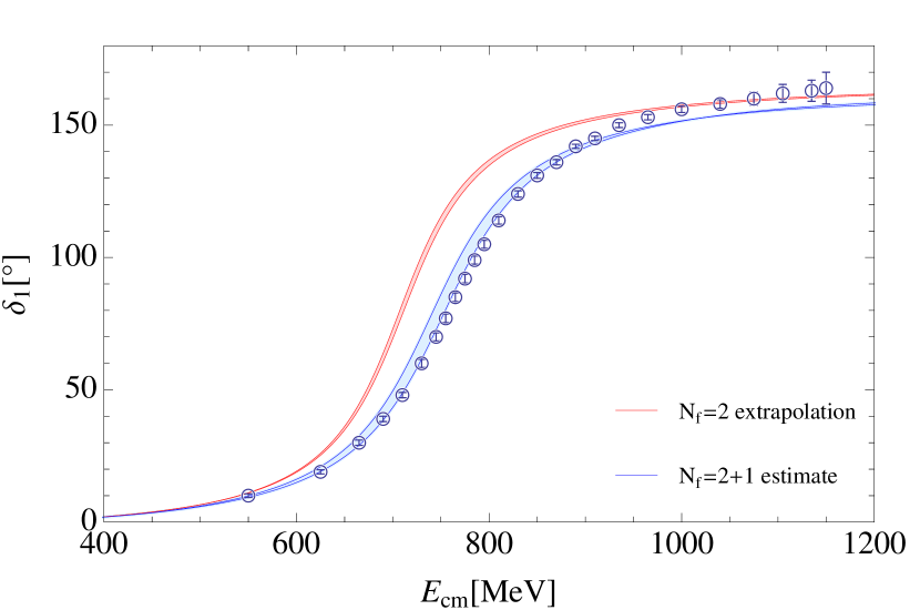
Figure 8: Chiral extrapolation of the phase shift to the physical mass (red band), obtained from the simultaneous fit to lattice eigenvalues at both considered pion masses. Only statistical uncertainties are indicated. The blue band shows the estimated phase shift when including also the $K\bar{K}$ channel in the two variants mentioned in the text. To keep the figure simple, statistical uncertainties are not indicated for these cases. They are of the same size as the red band. Open circles indicate phase shifts extracted from experiment Protopopescu et al. (1973).

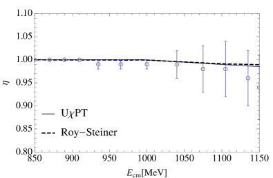
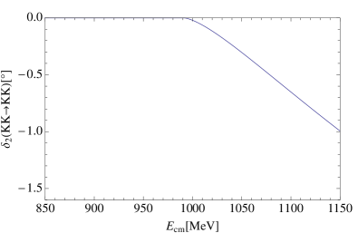
Figure 9: Left: Elasticity of $\pi\pi\to\pi\pi$ at physical pion masses compared with experimental determinations Protopopescu et al. (1973). The dashed line shows the inelasticity due to the $K\bar{K}$ channel alone as derived in reference Niecknig et al. (2012) from the Roy-Steiner solution in reference Buettiker et al. (2004). Right: Phase shift $\delta_{2}(K\bar{K}\to K\bar{K})$. In this figure we only show the result of variant 2 discussed in the text (results for variant 1 are very similar).

The combined U$\chi$PT fit to eigenvalues at both pion masses is discussed in Sec. III. We do not display the fit because it is almost indistinguishable from the blue curves in Fig. 5. The result of the chiral extrapolation is shown in Fig. 8 with the red band indicating the statistical uncertainties. The experimental data of Ref. Protopopescu et al. (1973) are depicted with circles. As one can see, the $N_{f}=2$ extrapolation remains far from the experimental data.

The two-channel U$\chi$PT formalism allows to estimate the effect of the missing strange quark in terms of the $K\bar{K}$ channel. For this, the $T$-matrix scattering amplitude, Eq. 59, is evaluated with the kernel $V$ from Eqs. 60, 67 and 68. The LECs in the $\pi\pi\to\pi\pi$ transition $\hat{l}_{1}$ and $\hat{l}_{2}$ are fixed at their values from the combined fit to the $N_{f}=2$ lattice data (see Table 4).

The combinations of LECs appearing in the $\pi\pi\to K\bar{K}$ and the $K\bar{K}\to K\bar{K}$ transitions of Eq. 68 are different from those of $\pi\pi\to\pi\pi$ and taken from a global fit to $\pi\pi$ and $\pi K$ experimental phase shift data, similar as in Ref. Döring et al. (2013). Statistical uncertainties from this source are not considered, because they are smaller than those from lattice data. The relevant values from this fit are $L_{3}=-3.01(2)\times 10^{-3}$ and $L_{5}=0.64(3)\times 10^{-3}$, $\hat{l}_{1}=0.26(5)\times 10^{-3}$, $\hat{l}_{2}=-3.96(4)\times 10^{-3}$.

However, note that $\hat{l}_{1}$ and $\hat{l}_{2}$ also appear in the $\pi\pi\to K\bar{K}$ and the $K\bar{K}\to K\bar{K}$ transitions (see Eq. 68). It is then not clear which values of $\hat{l}_{i}$ to use in these transitions. We have tested two variants:

1. Evaluate the $\pi\pi\to K\bar{K}$ and $K\bar{K}\to K\bar{K}$ transitions with the $\hat{l}_{1}$ and $\hat{l}_{2}$ from the fit to $N_{f}=2$ lattice data.

2. Set all the LECs involved in the $\pi\pi\to K\bar{K}$ and $K\bar{K}\to K\bar{K}$ transitions to the LECs from the mentioned fit to experimental data.

As Table 4 shows, the $\hat{l}_{i}$ from the fit to $N_{f}=2$ lattice data are similar to the ones quoted above, but not entirely compatible.

The result of the $2\to 3$ flavor extrapolation with these two variants is shown in Fig. 8 with the two blue curves connected by the blue band. The difference between these two strategies leads to about $20$ MeV difference in the mass of the $\rho(770)$ meson which gives an estimation of the uncertainties from model consistency.

Even though the $K\bar{K}$ channel has a significant impact on the mass of the $\rho$, the elasticity remains close to unity when this channel is open. This is shown in Fig. 9 (left). The $K\bar{K}$-phase shift is small and negative, as shown in Fig. 9 (right). It has the same sign as determined in Ref. Wilson et al. (2015) at an unphysical pion mass.

Before we conclude, we want to address a possible concern regarding the four-pion channel, which we believe to have a negligible effect on our results and conclusions. The effect is expected to be small because the branching ratio of $\rho$ to four pions is smaller than $2\times 10^{-3}$ Olive et al. (2014). The lattice simulation includes the four-pion channel and the U$\chi$PT model used here takes this effects into account only implicitly, through a shift in the values of the fitted low energy constants. At the simulation points the effect is thus, at least approximately, included and the main uncertainty comes from the chiral extrapolation. This is fundamentally different from the $K$-$\bar{K}$ channel which is absent in the lattice simulation. We believe that the uncertainty in the extrapolation is small, since the model fits our data at two different pion masses consistently and the extrapolation agrees very well, as can be seen from Fig. 6, with another $N_{f}=2$ lattice calculation very close to the physical point Bali et al. (2016).

In summary, even with the discussed theoretical uncertainty, the shift of the $\rho$ mass by the $K\bar{K}$ channel is significant and leads to a surprisingly good post-diction of experiment.

Appendix C Extracted energies and correlation matrices

In this section, we tabulate the details about fitting—fitting ansatz and fitting windows—for each energy level and for each ensemble used in this study. These details are reported in Table 6.

$m_{\pi}(\mathop{\hbox{MeV}})$	$\mathbf{P}$	$\eta$	$n$	ansatz	$t_{0}$	fit window	aE	$\chi^{2}$/dof	Q
$315$	$(0,0,0)$	$1.0$	$1$	$d$	$3$	$3-20$	0.4932(16)	0.65	$0.83$
			$2$	$d$	$3$	$5-15$	0.6612(14)	0.61	$0.77$
			$3$	$d$	$3$	$4-10$	0.842(4)	0.61	$0.65$
		$1.25$	$1$	$d$	$3$	$4-15$	0.4847(14)	1.5	$0.13$
			$2$	$d$	$3$	$5-14$	0.5891(14)	1.5	$0.16$
			$3$	$d$	$3$	$4-12$	0.785(5)	0.82	$0.55$
		$2.0$	$1$	$dc$	$3$	$4-16$	0.4508(6)	0.96	$0.47$
			$2$	$d$	$3$	$6-17$	0.5098(18)	1.23	$0.27$
			$3$	$d$	$3$	$5-15$	0.6547(13)	0.92	$0.49$
			$4$	$d$	$3$	$3-12$	0.704(2)	0.09	$0.99$
	$(0,0,1)$	$1.0$	$1$	$dt$	$3$	$5-17$	0.5024(8)	0.64	$0.77$
			$2$	$d$	$3$	$5-16$	0.5768(15)	0.47	$0.89$
			$3$	$d$	$3$	$3-13$	0.7492(15)	0.30	$0.96$
		$1.25$	$1$	$dt$	$3$	$7-15$	0.4701(9)	0.69	$0.63$
			$2$	$d$	$3$	$5-16$	0.547(2)	0.95	$0.47$
			$3$	$d$	$3$	$3-13$	0.717(2)	0.30	$0.97$
		$2.0$	$1$	$dt$	$3$	$3-20$	0.4241(7)	0.95	$0.50$
			$2$	$d$	$3$	$5-20$	0.5036(9)	1.36	$0.17$
			$3$	$d$	$3$	$5-17$	0.574(1)	0.38	$0.96$
			$4$	$d$	$3$	$3-13$	0.676(1)	0.37	$0.94$
$226$	$(0,0,0)$	$1.0$	$1$	$d$	$3$	$3-15$	0.4598(15)	0.82	$0.61$
			$2$	$d$	$3$	$3-12$	0.6184(15)	0.09	$0.99$
			$3$	$d$	$3$	$3-8$	0.820(8)	0.08	$0.97$
		$1.17$	$1$	$d$	$3$	$3-12$	0.448(2)	1.06	$0.39$
			$2$	$d$	$3$	$3-12$	0.558(2)	1.24	$0.28$
			$3$	$d$	$3$	$3-10$	0.744(18)	0.05	$0.99$
		$1.33$	$1$	$d$	$3$	$3-13$	0.4300(15)	0.44	$0.90$
			$2$	$d$	$3$	$3-14$	0.527(2)	0.35	$0.96$
			$3$	$d$	$3$	$3-11$	0.71(2)	0.08	$0.99$
	$(0,0,1)$	$1.0$	$1$	$d$	$3$	$6-18$	0.4217(9)	0.68	$0.75$
			$2$	$d$	$3$	$5-16$	0.5489(13)	0.68	$0.73$
			$3$	$d$	$3$	$3-12$	0.706(2)	0.19	$0.99$
		$1.17$	$1$	$d$	$3$	$6-20$	0.391(1)	0.32	$0.99$
			$2$	$d$	$3$	$3-12$	0.530(1)	0.88	$0.52$
			$3$	$d$	$3$	$3-10$	0.672(3)	0.70	$0.63$
		$1.33$	$1$	$dt$	$3$	$6-20$	0.371(1)	0.31	$0.98$
			$2$	$d$	$3$	$3-13$	0.5095(11)	0.97	$0.46$
			$3$	$d$	$3$	$3-11$	0.656(2)	0.17	$0.98$
			$4$	$d$	$3$	$3-11$	0.665(17)	1.09	$0.26$

Table 6: Extracted energies and fitting details. The ansatz labels the fitting function used; referring to Section III we have: d stands for double exponential function $f_{1}(t)$, dc is a double exponential function plus a constant term $f_{2}(t)$, and dt stands for its boosted variant $f_{3}(t)$. $Q$ is the confidence level of the fit, that is the probability under ideal conditions that the $\chi^{2}$ is larger than the fit result.

As we discussed in Section II.4, to determine resonance parameters by fitting a functional description to our phase-shifts we need to take into account cross-correlations between the extracted energies. The energies extracted from different ensembles are uncorrelated, but there will be correlations between the levels extracted from the same ensemble. We computed these covariance matrices using a jackknife procedure. These matrices are listed in Table 7.

$\left(\begin{array}[]{cccccc}24.8&1.76&5.95&3.34&2.43&3.47\\ &20.4&14.7&4.04&6.74&12.4\\ &&164&4.01&5.22&25.6\\ &&&6.8&2.67&4.16\\ &&&&23.4&3.74\\ &&&&&24.4\\ \end{array}\right)\times 10^{-7}$	$\left(\begin{array}[]{cccccc}24.0&-3.91&-34.0&4.0&3.6&-2.52\\ &23.8&71.0&3.57&4.02&10.0\\ &&760&-3.77&23.5&59.0\\ &&&8.71&1.18&3.17\\ &&&&15.9&-2.22\\ &&&&&41.0\\ \end{array}\right)\times 10^{-7}$
$\left(\begin{array}[]{cccccc}19.5&-2.03&-0.256&3.44&8.23&-2.92\\ &21.1&11.2&2.04&7.80&66.7\\ &&234&5.11&4.36&51.6\\ &&&8.34&2.63&0.536\\ &&&&30.0&0.269\\ &&&&&41.8\\ \end{array}\right)\times 10^{-7}$	$\left(\begin{array}[]{cccccc}33.9&-14.7&-44.4&1.09&5.67&-10.8\\ &43.1&145&1.60&2.56&22.3\\ &&2720&11.4&12.9&144\\ &&&9.73&0.885&2.98\\ &&&&12.1&-0.436\\ &&&&&68.2\\ \end{array}\right)\times 10^{-7}$
$\left(\begin{array}[]{cccccccc}3.62&2.24&1.54&1.87&3.16&3.10&1.90&1.74\\ &32.4&0.195&3.15&1.71&8.42&2.34&0.884\\ &&15.8&9.77&3.04&-0.063&9.99&6.21\\ &&&41.8&2.96&1.40&7.16&16.2\\ &&&&4.29&1.48&2.97&2.20\\ &&&&&9.57&0.90&0.222\\ &&&&&&10.1&4.62\\ &&&&&&&9.78\\ \end{array}\right)\times 10^{-7}$	$\left(\begin{array}[]{ccccccc}22.8&-5.91&-63.6&4.54&5.92&-3.50&-24.6\\ &42.8&108&3.80&5.21&18.6&32.9\\ &&5430&93.7&-29.2&32.6&1690\\ &&&19.3&2.78&1.62&57.4\\ &&&&14.2&2.45&-31.6\\ &&&&&39.9&-24.2\\ &&&&&&2820\\ \end{array}\right)\times 10^{-7}$

Table 7: Covariance matrices for the energies extracted from each ensembles. In the left column from top down we list the ensembles ${\cal E}_{1,2,3}$ corresponding to $m_{\pi}\approx 315\mathop{\hbox{MeV}}$ and on the right ${\cal E}_{4,5,6}$ corresponding to $m_{\pi}\approx 226\mathop{\hbox{MeV}}$. The order of the levels in each matrix corresponds to the order they appear in Table 6.

References

- Aoki et al. (2011a) S. Aoki et al. (PACS), Phys. Rev. D84, 094505 (2011a), arXiv:1106.5365 [hep-lat] .
- Göckeler et al. (2008) M. Göckeler, R. Horsley, Y. Nakamura, D. Pleiter, P. E. L. Rakow, G. Schierholz, and J. Zanotti (QCDSF), PoS LATTICE2008, 136 (2008), arXiv:0810.5337 [hep-lat] .
- Feng et al. (2011) X. Feng, K. Jansen, and D. B. Renner, Phys.Rev. D83, 094505 (2011), arXiv:1011.5288 [hep-lat] .
- Lang et al. (2011) C. Lang, D. Mohler, S. Prelovsek, and M. Vidmar, Phys.Rev. D84, 054503 (2011), arXiv:1105.5636 [hep-lat] .
- Pelissier and Alexandru (2013) C. Pelissier and A. Alexandru, Phys.Rev. D87, 014503 (2013), arXiv:1211.0092 [hep-lat] .
- Bali et al. (2016) G. S. Bali, S. Collins, A. Cox, G. Donald, M. Göckeler, C. B. Lang, and A. Schäfer (RQCD), Phys. Rev. D93, 054509 (2016), arXiv:1512.08678 [hep-lat] .
- Frison et al. (2010) J. Frison et al. (Budapest-Marseille-Wuppertal), PoS LATTICE2010, 139 (2010), arXiv:1011.3413 [hep-lat] .
- Dudek et al. (2013) J. J. Dudek, R. G. Edwards, and C. E. Thomas (Hadron Spectrum), Phys.Rev. D87, 034505 (2013), arXiv:1212.0830 [hep-ph] .
- Metivet (2015) T. Metivet (Budapest-Marseille-Wuppertal), PoS LATTICE2014, 079 (2015), arXiv:1410.8447 [hep-lat] .
- Wilson et al. (2015) D. J. Wilson, R. A. Briceño, J. J. Dudek, R. G. Edwards, and C. E. Thomas, (2015), arXiv:1507.02599 [hep-ph] .
- Bulava et al. (2016) J. Bulava, B. Fahy, B. Hörz, K. J. Juge, C. Morningstar, and C. H. Wong, (2016), arXiv:1604.05593 [hep-lat] .
- Feng et al. (2015) X. Feng, S. Aoki, S. Hashimoto, and T. Kaneko, Phys. Rev. D91, 054504 (2015), arXiv:1412.6319 [hep-lat] .
- Lüscher (1986a) M. Lüscher, Commun.Math.Phys. 104, 177 (1986a).
- Lüscher (1986b) M. Lüscher, Commun.Math.Phys. 105, 153 (1986b).
- Lüscher and Wolff (1990) M. Lüscher and U. Wolff, Nucl.Phys. B339, 222 (1990).
- Lüscher (1991) M. Lüscher, Nucl.Phys. B354, 531 (1991).
- Rummukainen and Gottlieb (1995) K. Rummukainen and S. A. Gottlieb, Nucl. Phys. B450, 397 (1995), arXiv:hep-lat/9503028 [hep-lat] .
- Feng et al. (2004) X. Feng, X. Li, and C. Liu, Phys.Rev. D70, 014505 (2004), arXiv:hep-lat/0404001 [hep-lat] .
- Hasenfratz et al. (2007) A. Hasenfratz, R. Hoffmann, and S. Schaefer, JHEP 0705, 029 (2007), arXiv:hep-lat/0702028 [hep-lat] .
- Peardon et al. (2009) M. Peardon, J. Bulava, J. Foley, C. Morningstar, J. Dudek, R. G. Edwards, B. Joo, H.-W. Lin, D. G. Richards, and K. J. Juge (Hadron Spectrum), Phys. Rev. D80, 054506 (2009), arXiv:0905.2160 [hep-lat] .
- Oller et al. (1999) J. A. Oller, E. Oset, and J. R. Pelaez, Phys. Rev. D59, 074001 (1999), [Erratum: Phys. Rev.D75,099903(2007)], arXiv:hep-ph/9804209 [hep-ph] .
- Döring et al. (2011) M. Döring, U.-G. Meißner, E. Oset, and A. Rusetsky, Eur. Phys. J. A47, 139 (2011), arXiv:1107.3988 [hep-lat] .
- Pelissier et al. (2011) C. Pelissier, A. Alexandru, and F. X. Lee, PoS LATTICE2011, 134 (2011), arXiv:1111.2314 [hep-lat] .
- Blossier et al. (2009) B. Blossier, M. Della Morte, G. von Hippel, T. Mendes, and R. Sommer, JHEP 0904, 094 (2009), arXiv:0902.1265 [hep-lat] .
- Moore and Fleming (2006) D. C. Moore and G. T. Fleming, Phys.Rev. D73, 014504 (2006), arXiv:hep-lat/0507018 [hep-lat] .
- Morningstar et al. (2011) C. Morningstar, J. Bulava, J. Foley, K. J. Juge, D. Lenkner, et al., Phys.Rev. D83, 114505 (2011), arXiv:1104.3870 [hep-lat] .
- Alexandru et al. (2012) A. Alexandru, C. Pelissier, B. Gamari, and F. Lee, J. Comput. Phys. 231, 1866 (2012), arXiv:1103.5103 [hep-lat] .
- Lüscher and Weisz (1985) M. Lüscher and P. Weisz, Commun.Math.Phys. 97, 59 (1985).
- Alford et al. (1995) M. G. Alford, W. Dimm, G. Lepage, G. Hockney, and P. Mackenzie, Phys.Lett. B361, 87 (1995), arXiv:hep-lat/9507010 [hep-lat] .
- Lüscher (2010) M. Lüscher, JHEP 1008, 071 (2010), arXiv:1006.4518 [hep-lat] .
- Borsanyi et al. (2012) S. Borsanyi, S. Durr, Z. Fodor, C. Hoelbling, S. D. Katz, et al., (2012), arXiv:1203.4469 [hep-lat] .
- Bruno and Sommer (2014) M. Bruno and R. Sommer (ALPHA), PoS LATTICE2013, 321 (2014), arXiv:1311.5585 [hep-lat] .
- Fritzsch et al. (2012) P. Fritzsch, F. Knechtli, B. Leder, M. Marinkovic, S. Schaefer, R. Sommer, and F. Virotta, Nucl. Phys. B865, 397 (2012), arXiv:1205.5380 [hep-lat] .
- Sommer (1994) R. Sommer, Nucl.Phys. B411, 839 (1994), arXiv:hep-lat/9310022 [hep-lat] .
- Yang et al. (2014) Y.-B. Yang, Y. Chen, A. Alexandru, S.-J. Dong, T. Draper, et al., (2014), arXiv:1410.3343 [hep-lat] .
- Aoki et al. (2011b) Y. Aoki et al. (RBC, UKQCD), Phys. Rev. D83, 074508 (2011b), arXiv:1011.0892 [hep-lat] .
- Walker-Loud (2008) A. Walker-Loud, PoS LATTICE2008, 005 (2008), arXiv:0810.0663 [hep-lat] .
- Durr et al. (2011) S. Durr, Z. Fodor, C. Hoelbling, S. Katz, S. Krieg, et al., JHEP 1108, 148 (2011), arXiv:1011.2711 [hep-lat] .
- Prelovsek and Mohler (2009) S. Prelovsek and D. Mohler, Phys. Rev. D79, 014503 (2009), arXiv:0810.1759 [hep-lat] .
- Dudek et al. (2012) J. J. Dudek, R. G. Edwards, and C. E. Thomas, Phys.Rev. D86, 034031 (2012), arXiv:1203.6041 [hep-ph] .
- von Hippel and Quigg (1972) F. von Hippel and C. Quigg, Phys. Rev. D 5, 624 (1972).
- Bruns and Meissner (2005) P. C. Bruns and U.-G. Meissner, Eur. Phys. J. C40, 97 (2005), arXiv:hep-ph/0411223 [hep-ph] .
- Note (1) There is lattice QCD evidence that the mass of is well described by a linear dependence on near the physical quark mass below Chen et al. (2015).
- Hu et al. (2016) B. Hu, R. Molina, M. Doering, and A. Alexandru, “Two-flavor Simulations of the (770) and the Role of the Channel,” (2016), in preparation.
- Pelaez and Rios (2010) J. R. Pelaez and G. Rios, Phys. Rev. D82, 114002 (2010), arXiv:1010.6008 [hep-ph] .
- Olive et al. (2014) K. A. Olive et al. (Particle Data Group), Chin. Phys. C38, 090001 (2014).
- Li and Liu (2004) X. Li and C. Liu, Phys.Lett. B587, 100 (2004), arXiv:hep-lat/0311035 [hep-lat] .
- Gasser and Leutwyler (1984) J. Gasser and H. Leutwyler, Annals Phys. 158, 142 (1984).
- Gasser and Leutwyler (1985) J. Gasser and H. Leutwyler, Nucl. Phys. B250, 465 (1985).
- Truong (1988) T. N. Truong, Phys. Rev. Lett. 61, 2526 (1988).
- Dobado et al. (1990) A. Dobado, M. J. Herrero, and T. N. Truong, Phys. Lett. B235, 134 (1990).
- Dobado and Pelaez (1993) A. Dobado and J. R. Pelaez, Phys. Rev. D47, 4883 (1993), arXiv:hep-ph/9301276 [hep-ph] .
- Dobado and Pelaez (1997) A. Dobado and J. R. Pelaez, Phys. Rev. D56, 3057 (1997), arXiv:hep-ph/9604416 [hep-ph] .
- Nebreda and Pelaez. (2010) J. Nebreda and J. R. Pelaez., Phys. Rev. D81, 054035 (2010), arXiv:1001.5237 [hep-ph] .
- Doring et al. (2011) M. Doring, J. Haidenbauer, U.-G. Meissner, and A. Rusetsky, Eur. Phys. J. A47, 163 (2011), arXiv:1108.0676 [hep-lat] .
- Doring et al. (2009) M. Doring, C. Hanhart, F. Huang, S. Krewald, and U. G. Meissner, Phys. Lett. B681, 26 (2009), arXiv:0903.1781 [nucl-th] .
- Martinez Torres et al. (2012) A. Martinez Torres, L. R. Dai, C. Koren, D. Jido, and E. Oset, Phys. Rev. D85, 014027 (2012), arXiv:1109.0396 [hep-lat] .
- Doring et al. (2012) M. Doring, U. G. Meissner, E. Oset, and A. Rusetsky, Eur. Phys. J. A48, 114 (2012), arXiv:1205.4838 [hep-lat] .
- Protopopescu et al. (1973) S. D. Protopopescu, M. Alston-Garnjost, A. Barbaro-Galtieri, S. M. Flatte, J. H. Friedman, T. A. Lasinski, G. R. Lynch, M. S. Rabin, and F. T. Solmitz, Phys. Rev. D7, 1279 (1973).
- Niecknig et al. (2012) F. Niecknig, B. Kubis, and S. P. Schneider, Eur. Phys. J. C72, 2014 (2012), arXiv:1203.2501 [hep-ph] .
- Buettiker et al. (2004) P. Buettiker, S. Descotes-Genon, and B. Moussallam, Eur. Phys. J. C33, 409 (2004), arXiv:hep-ph/0310283 [hep-ph] .
- Döring et al. (2013) M. Döring, U.-G. Meißner, and W. Wang, JHEP 10, 011 (2013), arXiv:1307.0947 [hep-ph] .
- Chen et al. (2015) Y. Chen, A. Alexandru, T. Draper, K.-F. Liu, Z. Liu, and Y.-B. Yang, (2015), arXiv:1507.02541 [hep-ph] .