Equivariant Perturbation in
Gomory and Johnson’s Infinite Group Problem.
VI. The Curious Case of Two-Sided Discontinuous Minimal Valid Functions

Abstract.

We construct a two-sided discontinuous piecewise linear minimal valid cut-generating function for the 1-row Gomory–Johnson model which is not extreme, but which is not a convex combination of other piecewise linear minimal valid functions. The new function only admits piecewise microperiodic perturbations. We present an algorithm for verifying certificates of non-extremality in the form of such perturbations.

1. Introduction

1.1. Continuous and discontinuous functions related to corner polyhedra

Gomory and Johnson, in their seminal papers [11, 12] titled Some continuous functions related to corner polyhedra I, II, introduced piecewise linear functions that are related to Gomory’s group relaxation [10] of integer linear optimization problems. Let $f\in(0,1)$ be a fixed number and consider the solutions in non-negative integer variables $y_{j}$ to an equation (the group relaxation) of the form

$$\sum_{j=1}^{m}r_{j}y_{j}\equiv f\pmod{1},$$ (1)

where $r_{j}\in\mathbb{R}$ are given coefficients. A cutting plane, or valid inequality, is a linear inequality that is satisfied by all non-negative integer solutions $y$. A classical method of deriving cutting planes, the Gomory mixed-integer cut, can be expressed as follows. Consider the function $\pi=\href https://github.com/mkoeppe/infinite-group-relaxation-code/search?q=$ as the piecewise linear function that is the $\mathbb{Z}$-periodic extension of the linear interpolation of $\pi(0)=0$, $\pi(f)=1$, and $\pi(1)=0$. Then

$$\sum_{j=1}^{m}\pi(r_{j})y_{j}\geq 1$$ (2)

is a valid inequality. What is remarkable is that the function $\pi$ only depends on a single parameter (the right-hand side $f$) and can be applied to any equation of the form (1), no matter what the given coefficients $r_{j}$ are; moreover, it provides the coefficients $\pi(r_{j})$ of the cutting plane independently of each other. Nowadays, following Conforti et al. [7], we call functions $\pi$ of this type cut-generating functions.

Another classical cutting plane, the Gomory fractional cut, can be described using this pattern. Its cut-generating function $\pi=\href https://github.com/mkoeppe/infinite-group-relaxation-code/search?q=$, considered as a function from the reals to the reals, is a sawtooth function, discontinuous at all integers. However, Gomory and Johnson considered these functions as going from the interval $[0,1)$, essentially removing the discontinuities from any further analysis. Besides, in the hierarchy of cut-generating functions, arranged by increasing strength from valid over subadditive and minimal to extreme and facet, the gomory_fractional function belongs to the category of merely subadditive functions. As is well-known, it is dominated by the Gomory mixed-integer cut, whose cut-generating function gmic is a continuous extreme function. This may explain Gomory and Johnson’s focus on the continuous functions of their papers’ titles. In their papers, they gave a full characterization of the minimal functions (they are the $\mathbb{Z}$-periodic, subadditive functions $\pi\colon\mathbb{R}\to\mathbb{R}_{+}$ with $\pi(0)=0$ that satisfy the symmetry condition $\pi(x)+\pi(f-x)=1$ for all $x\in\mathbb{R}$). Among the minimal functions, a function is extreme if it cannot be written as a convex combination of two other minimal functions. Gomory and Johnson initiated a classification program for (continuous) extreme functions, an early success of which was the two-slope theorem, asserting that every continuous piecewise linear minimal function whose derivatives take only two values is already extreme. This was a vast generalization of the extremality of the Gomory mixed-integer cut. In parts of the later literature, the related notion of facets, instead of extreme functions, was considered; see [16].

Undisputably discontinuous functions came into play 30 years later, when Letchford–Lodi [17] introduced their strong fractional cut (ll_strong_fractional ) as a strengthening of the gomory_fractional cut. (It neither dominates nor is dominated by the gmic function.) Letchford and Lodi first prove, by elementary means, that their new cutting plane gives a valid inequality; then they remark:

[The] function mapping the coefficients of [the source row] onto the coefficients in the strong fractional cut […] can be shown to be subadditive. It also meets the other conditions of [Gomory–Johnson’s characterization of minimal valid functions]. However, it differs from the subadditive functions given in [Gomory–Johnson’s papers] in that it is discontinuous.

Further study of discontinuous functions took place in the context of pointwise limits of continuous functions. Dash and Günlük [8] introduced extended two-step MIR (mixed integer rounding) inequalities (dg_2_step_mir_limit ), whose corresponding cut-generating functions arise as limits of sequences of two-step MIR functions (dg_2_step_mir ) defined in the same paper. They showed that these functions, up to automorphism, give cutting planes that dominate the Letchford–Lodi strong fractional cuts. Dey, Richard, Li, and Miller [9] were the first to consider discontinuous functions as first-class members of the Gomory–Johnson hierarchy of valid functions, and introduced important tools for their study. They identified Dash and Günlük’s family dg_2_step_mir_limit as extreme functions, introduced the enclosing family drlm_2_slope_limit , and defined another family of discontinuous functions, drlm_3_slope_limit . Later Richard, Li, and Miller [18] conducted a systematic study of discontinuous functions via the connection to superadditive lifting functions, which brought examples such as rlm_dpl1_extreme_3a .

1.2. The rôle of one-sided continuity in testing extremality

Note that all of the above-mentioned families of extreme functions are one-sided continuous at the origin, either from the left or from the right. To explain the significance of this observation, we will outline the structure of an extremality proof, using the notion of effective perturbations introduced in [14, 15]. Let $\pi\colon\mathbb{R}\to\mathbb{R}_{+}$ be a minimal valid function. Suppose $\pi=\frac{1}{2}(\pi^{1}+\pi^{2})$ where $\pi^{1}$ and $\pi^{2}$ are valid functions; then $\pi^{1}$ and $\pi^{2}$ are minimal. Write $\pi^{1}=\pi+\varepsilon\tilde{\pi}$ and $\pi^{2}=\pi-\varepsilon\tilde{\pi}$, where $\tilde{\pi}\colon\mathbb{R}\to\mathbb{R}$ and $\varepsilon>0$; then we call $\tilde{\pi}$ an effective perturbation function. Towards the goal of showing $\tilde{\pi}=0$, one asks the following.

Question 1.0.

Given a minimal function $\pi$, what properties does an effective perturbation $\tilde{\pi}$ necessarily have?

Later in this paper we will review answers to this question, which include the boundedness of $\tilde{\pi}$, the inheritance of additivity (see 2.0 below) and linearity properties (see Theorem 2.1 and Theorem 3.2 below). For now, we will focus on the following important regularity lemma by Dey, Richard, Li, and Miller [9], which makes an assumption of one-sided continuity at the origin. It is a consequence of subadditivity of minimal functions and serves as a crucial ingredient of many extremality proofs.

Lemma 1.0 ([9, Theorem 2]; see [4, Lemma 2.11 (v)]).

Let $\pi\colon\mathbb{R}\to\mathbb{R}_{+}$ be a minimal valid function and $\tilde{\pi}$ an effective perturbation. If $\pi$ is piecewise linear and continuous from the right at $0$ or from the left at $0$, then $\tilde{\pi}$ is continuous at all points at which $\pi$ is continuous.

Hildebrand (2013, unpublished; see [4]), constructed the first examples of extreme functions that are two-sided discontinuous at the origin, hildebrand_2_sided_discont_1_slope_1 , hildebrand_2_sided_discont_2_slope_1 . Their extremality proofs do not depend on 1.0. Later, Zhou [20] constructed the first example, zhou_two_sided_discontinuous_cannot_assume_any_continuity (Figure 1), that demonstrates that the hypothesis of one-sided continuity at the origin cannot be removed from 1.0.

Figure 1. This function, $\pi$ = zhou_two_sided_discontinuous_cannot_assume_any_continuity, is minimal, but not extreme, as proved by extremality_test($\pi$, show_plots=True). The procedure first shows that for any distinct minimal $\pi^{1}=\pi+\bar{\pi}$ (blue), $\pi^{2}=\pi-\bar{\pi}$ (red) such that $\pi=\tfrac{1}{2}\pi^{1}+\tfrac{1}{2}\pi^{2}$, the functions $\pi^{1}$ and $\pi^{2}$ are piecewise linear with the same breakpoints as $\pi$ and possible additional breakpoints at $\frac{1}{4}$ and $\frac{3}{4}$. The open intervals between these breakpoints are covered (see section 2, after Theorem 2.1, for this notion). A finite-dimensional extremality test then finds exactly one linearly independent perturbation $\bar{\pi}$ (magenta), as shown. Thus all nontrivial perturbations are discontinuous at $\frac{3}{4}$, a point where $\pi$ is continuous.

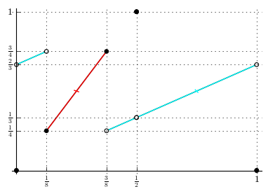
The breakdown of the regularity lemma in the two-sided discontinuous case poses a challenge for the algorithmic theory of extreme functions. Consider the following variant of 1.0:

Question 1.0.

(a) What class of effective perturbations $\tilde{\pi}$ is sufficient to certify the non-extremality of all non-extreme piecewise linear functions? (b) In particular, do piecewise linear effective perturbations $\tilde{\pi}$ suffice?

For the case of piecewise linear functions $\pi$ with rational breakpoints from $\frac{1}{q}\mathbb{Z}$, Basu et al. [3], in the first paper in the present series then showed that if a nonzero effective perturbation exists, there also exists one that is piecewise linear with rational breakpoints in $\frac{1}{4q}\mathbb{Z}$. This implied the first algorithm for testing the extremality of a (possibly discontinuous) piecewise linear minimal valid function with rational breakpoints. In the same paper, however, Basu et al. [3] also introduced a family bhk_irrational of continuous piecewise linear minimal valid functions with irrational breakpoints, to which the algorithm does not apply. Its extremality proof uses an arithmetic argument that depends on the $\mathbb{Q}$-linear independence of certain parameters of the function, and also relies on 1.0.

Figure 2. This function, $\pi$ = kzh_minimal_has_only_crazy_perturbation_1, has three slopes (blue, green, red) and is discontinuous on both sides of the origin. It is a non-extreme minimal valid function, but in order to demonstrate non-extremality, one needs to use a highly discontinuous (locally microperiodic) perturbation. We construct a simple explicit example perturbation $\varepsilon\bar{\pi}$ (magenta); see Theorem 5.1. It takes three values, $\varepsilon$, $0$, and $-\varepsilon$ (horizontal magenta line segments) where $\varepsilon=0.0003$; in the figure it has been rescaled to amplitude $\frac{1}{10}$.

1.3. Contributions of this paper

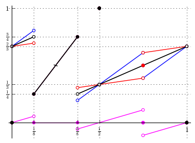
In the present paper, we show that the breakdown of the regularity lemma (1.0) does not just pose a technical difficulty; rather, two-sided discontinuous functions take an exceptional place in the theory of the Gomory–Johnson functions. We construct a two-sided discontinuous piecewise linear minimal valid function $\pi$ with remarkable properties; cf. Figure 2. It follows the basic blueprint of the bhk_irrational function that we mentioned above, but introduces a number of discontinuities and new breakpoints. Our function $\pi=\href https://github.com/mkoeppe/infinite-group-relaxation-code/search?q=$ is not extreme, but it is impossible to write it as the convex combination of piecewise linear (or, more generally, piecewise continuous) minimal valid functions. All effective perturbations $\tilde{\pi}$ of $\pi$ are non–piecewise linear, highly discontinuous, “locally microperiodic” functions. Thus, we give a negative answer to 1.0 (b): Piecewise linear effective perturbations do not suffice to certify nonextremality of piecewise linear functions. (Moreover, in the authors’ IPCO 2017 paper [16], building upon the present paper, the function $\pi$ and a certain perturbation of it are instrumental in separating the classes of extreme functions, facets, and so-called weak facets, thereby solving the long-standing open question [4, Open question 2.9] regarding the relations of these notions.)

In this way, our paper contributes to the foundations of the cutting-plane theory of integer programming by investigating the fine structure of a space of cut-generating functions. In this regard, the paper is in a line of recent papers on the Gomory–Johnson model: the MPA 2012 paper [1], in which the first non–piecewise linear, measurable extreme function with 2 slopes was discovered; and the IPCO 2016 paper [2], in which a measurable extreme function with an infinite number of slopes was constructed using techniques similar to those in [1].

However, our paper not only constructs an example, but also develops the theory of effective perturbations of minimal valid functions further. Local continuity of perturbations has been observed and used in the original Gomory–Johnson papers [11, 12]. The extension to the one-sided discontinuous case (1.0) was found by Dey, Richard, Li, and Miller [9]. We prove a new analytical tool. Our Theorem 3.1 establishes the existence of one-sided or two-sided limits of effective perturbation functions $\tilde{\pi}$ at certain points, providing a weak counterpart of 1.0 without the assumption of one-sided continuity of $\pi$. We consider our Theorem 3.1 to be a major advance, requiring a much more subtle proof. (For comparison, see the short proof of a stronger version of 1.0, establishing Lipschitz continuity of $\tilde{\pi}$ on the intervals of continuity of $\pi$, in [15, Lemma 6.4].) We leave as an open question how to generalize Theorem 3.1 to the multi-row case [6], i.e., functions $\pi\colon\mathbb{R}^{k}\to\mathbb{R}$.

Our paper is structured as follows. In section 2, we introduce notation, definitions, and basic results from the literature. In section 3, we prove our result on the existence of limits. In section 4, in order to demonstrate the nonextremality of the new function $\pi$, we develop an algorithm to verify a certificate of nonextremality in the form of a given locally quasimicroperiodic function $\bar{\pi}$ of a restricted class. In section 5, we define the example functions $\pi$ and $\bar{\pi}$ and prove that they have the claimed properties. The complexity of this proof is much greater than that of functions from the extreme functions literature; because of this, our proof is computer-assisted.

2. Preliminaries

We begin by giving a definition of $\mathbb{Z}$-periodic piecewise linear functions $\pi\colon\mathbb{R}\to\mathbb{R}$ that are allowed to be discontinuous, following [3, section 2.1] and the recent survey [4, 5].

Let $0=x_{0}<x_{1}<\dots<x_{n-1}<x_{n}=1$. Denote by $B=\{\,x_{0}+t,x_{1}+t,\dots,x_{n-1}+t\mid t\in\mathbb{Z}\,\}$ the set of all breakpoints. The 0-dimensional faces are defined to be the singletons, $\{x\}$, $x\in B$, and the 1-dimensional faces are the closed intervals, $[x_{i}+t,x_{i+1}+t]$, $i=0,\dots,{n-1}$, $t\in\mathbb{Z}$. The empty face, the 0-dimensional and the 1-dimensional faces form $\mathcal{P}=\mathcal{P}_{B}$, a locally finite polyhedral complex, periodic modulo $\mathbb{Z}$. We call a function $\pi\colon\mathbb{R}\to\mathbb{R}$ piecewise linear over $\mathcal{P}_{B}$ if for each face $I\in\mathcal{P}_{B}$, there is an affine linear function $\pi_{I}\colon\mathbb{R}\to\mathbb{R}$, $\pi_{I}(x)=c_{I}x+d_{I}$ such that $\pi(x)=\pi_{I}(x)$ for all $x\in\operatorname{rel\,int}(I)$. Under this definition, piecewise linear functions can be discontinuous. Let $I=[a,b]\in\mathcal{P}_{B}$ be a 1-dimensional face. The function $\pi$ can be determined on $\operatorname{int}(I)=(a,b)$ by linear interpolation of the limits $\pi(a^{+})=\lim_{x\to a,x>a}\pi(x)=\pi_{I}(a)$ and $\pi(b^{-})=\lim_{x\to b,x<b}\pi(x)=\pi_{I}(b)$. Likewise, we call a function $\pi\colon\mathbb{R}\to\mathbb{R}$ piecewise continuous over $\mathcal{P}_{B}$ if it is continuous over $\operatorname{rel\,int}(I)$ for each face $I\in\mathcal{P}_{B}$.

The minimal valid functions in the classic 1-row Gomory–Johnson [11, 12] model are classified. They are the $\mathbb{Z}$-periodic, subadditive functions $\pi\colon\mathbb{R}\to[0,1]$ with $\pi(0)=0$, $\pi(f)=1$, that satisfy the symmetry condition $\pi(x)+\pi(f-x)=1$ for all $x\in\mathbb{R}$. Here $f$ is the fixed number from (1). Following [3, 4, 5], we introduce the function

$$\Delta\pi\colon\mathbb{R}\times\mathbb{R}\to\mathbb{R},\quad\Delta\pi(x,y)=\pi(x)+\pi(y)-\pi(x+y),$$

which measures the slack in the subadditivity condition. If $\pi(x)$ is piecewise linear, then this induces the piecewise linearity of $\Delta\pi(x,y)$. To express the domains of linearity of $\Delta\pi(x,y)$, and thus domains of additivity and strict subadditivity, we introduce the two-dimensional polyhedral complex $\Delta\mathcal{P}=\Delta\mathcal{P}_{B}$. The faces $F$ of the complex are defined as follows. Let $I,J,K\in\mathcal{P}_{B}$, so each of $I,J,K$ is either the empty set, a breakpoint of $\pi$, or a closed interval delimited by two consecutive breakpoints. Then

$$F=F(I,J,K)=\left\{\,(x,y)\in\mathbb{R}\times\mathbb{R}\,\mid\,x\in I,\,y\in J,\,x+y\in K\,\right\}.$$

The projections $p_{1},p_{2},p_{3}\colon\mathbb{R}\times\mathbb{R}\to\mathbb{R}$ are defined as $p_{1}(x,y)=x$, $p_{2}(x,y)=y$, $p_{3}(x,y)=x+y$.

Let $F\in\Delta\mathcal{P}$ and let $(u,v)\in F$. Observing that $\Delta\pi|_{\operatorname{rel\,int}(F)}$ is affine, we define

$$\Delta\pi_{F}(u,v)=\lim_{\begin{subarray}{c}(x,y)\to(u,v)\\ (x,y)\in\operatorname{rel\,int}(F)\end{subarray}}\Delta\pi(x,y),$$ (3)

which allows us to conveniently express limits to boundary points of $F$, in particular to vertices of $F$, along paths within $\operatorname{rel\,int}(F)$. It is clear that $\Delta\pi_{F}(u,v)$ is affine over $F$, and $\Delta\pi(u,v)=\Delta\pi_{F}(u,v)$ for all $(u,v)\in\operatorname{rel\,int}(F)$. We will use $\operatorname{vert}(F)$ to denote the set of vertices of the face $F$.

Let $\pi$ be a piecewise linear minimal valid function. We now define the additive faces of the two-dimensional polyhedral complex $\Delta\mathcal{P}$ of $\pi$. When $\pi$ is continuous, we say that a face $F\in\Delta\mathcal{P}$ is additive if $\Delta\pi=0$ over all $F$. Note that $\Delta\pi$ is affine over $F$, so the condition is equivalent to $\Delta\pi(u,v)=0$ for any $(u,v)\in\operatorname{vert}(F)$. When $\pi$ is discontinuous, following [14, 15], we say that a face $F\in\Delta\mathcal{P}$ is additive if $F$ is contained in a face $F^{\prime}\in\Delta\mathcal{P}$ such that $\Delta\pi_{F^{\prime}}(x,y)=0$ for any $(x,y)\in F$. Since $\Delta\pi$ is affine in the relative interiors of each face of $\Delta\mathcal{P}$, the last condition is equivalent to $\Delta\pi_{F^{\prime}}(u,v)=0$ for any $(u,v)\in\operatorname{vert}(F)$.

A minimal valid function $\pi$ is said to be extreme if it cannot be written as a convex combination of two other minimal valid functions. We say that a function $\tilde{\pi}$ is an effective perturbation function for the minimal valid function $\pi$, denoted $\tilde{\pi}\in\tilde{\Pi}^{\pi}(\mathbb{R},\mathbb{Z})$, if there exists $\varepsilon>0$ such that $\pi\pm\varepsilon\tilde{\pi}$ are minimal valid functions. Thus, a minimal valid function $\pi$ is extreme if and only if no non-zero effective perturbation $\tilde{\pi}\in\tilde{\Pi}^{\pi}(\mathbb{R},\mathbb{Z})$ exists.

The key technique towards answering 1.0 is to analyze the additivity relations. The starting point is the following lemma, which shows that all subadditivity conditions that are tight (satisfied with equality) for $\pi$ are also tight for an effective perturbation $\tilde{\pi}$. This includes additivity in the limit, which we express using the notation $\Delta\tilde{\pi}_{F}$, defined as a limit as in (3), though $\tilde{\pi}$ is not assumed to be piecewise linear.

Lemma 2.0 ([3, Lemma 2.7]; see [15, Lemma 6.1]).

Let $\pi$ be a minimal valid function that is piecewise linear over $\mathcal{P}$. Let $F$ be a face of $\Delta\mathcal{P}$ and let $(u,v)\in F$. If $\Delta\pi_{F}(u,v)=0$, then $\Delta\tilde{\pi}_{F}(u,v)=0$ for any effective perturbation function $\tilde{\pi}\in\tilde{\Pi}^{\pi}(\mathbb{R},\mathbb{Z})$.

We first make use of the additivity relations that are captured by the two-dimensional additive faces $F$ of $\Delta\mathcal{P}$. The following, a corollary of the convex additivity domain lemma [4, Theorem 4.3], appears as [15, Theorem 6.2].

Theorem 2.1.

Let $\pi$ be a minimal valid function that is piecewise linear over $\mathcal{P}$. Let $F$ be a two-dimensional additive face of $\Delta\mathcal{P}$. Let $\theta=\pi$ or $\theta=\tilde{\pi}\in\tilde{\Pi}^{\pi}(\mathbb{R},\mathbb{Z})$. Then $\theta$ is affine with the same slope over $\operatorname{int}(p_{1}(F))$, $\operatorname{int}(p_{2}(F))$, and $\operatorname{int}(p_{3}(F))$.

In the situation of this result, we say that the intervals $\operatorname{int}(p_{1}(F))$, $\operatorname{int}(p_{2}(F))$, and $\operatorname{int}(p_{3}(F))$ are (directly) covered and are in the same connected covered component. Subintervals of covered intervals are covered.

In addition to directly covered intervals, we also have indirectly covered intervals, which arise from vertical, horizontal, or diagonal additive edges $F$ of $\Delta\mathcal{P}$. To handle these additive edges in our setting of two-sided discontinuous functions with irrational breakpoints, we need a new technical tool, which we develop in the following section.

3. Existence of limits of effective perturbations at certain points and a general additive edge theorem

The following main theorem is our weak counterpart of the regularity lemma, 1.0, which does not require the assumption of one-sided continuity.

Theorem 3.1.

Let $\pi$ be a minimal valid function that is piecewise linear over a complex $\mathcal{P}$. Let $\tilde{\pi}\in\tilde{\Pi}^{\pi}(\mathbb{R},\mathbb{Z})$ be an effective perturbation function for $\pi$. If a point $(u,v)$ in a two-dimensional face $F\in\Delta\mathcal{P}$ satisfies that $\Delta\pi_{F}(u,v)=0$, then the limits

$$\lim_{\begin{subarray}{c}x\to u\\ x\in\operatorname{int}(p_{1}(F))\end{subarray}}\tilde{\pi}(x),\quad\lim_{\begin{subarray}{c}y\to v\\ y\in\operatorname{int}(p_{2}(F))\end{subarray}}\tilde{\pi}(y)\quad\text{ and }\quad\lim_{\begin{subarray}{c}z\to u+v\\ z\in\operatorname{int}(p_{3}(F))\end{subarray}}\tilde{\pi}(z)$$

exist.

It is convenient to first prove the following “pexiderized” [6] proposition.

Proposition 3.1.

Let $F$ be a two-dimensional face of $\Delta\mathcal{P}$, where $\mathcal{P}$ is the one-dimensional polyhedral complex of a piecewise linear function. Let $(u,v)\in F$. For $i=1,2,3$, let $\tilde{\pi}_{i}\colon\mathbb{R}\to\mathbb{R}$ be a function that is bounded near $p_{i}(u,v)$. If

$$\lim_{\begin{subarray}{c}(x,y)\to(u,v)\\ (x,y)\in\operatorname{int}(F)\end{subarray}}{\tilde{\pi}_{1}(x)+\tilde{\pi}_{2}(y)-\tilde{\pi}_{3}(x+y)}=0,$$

then for $i=1,2,3$, the limit $\lim_{t\to p_{i}(u,v),\;t\in\operatorname{int}(p_{i}(F))}\tilde{\pi}_{i}(t)$ exists.

Proof.

We will prove the following claim.

Claim. For $i=1,2,3$ and every $\varepsilon>0$, there exists a neighborhood $N_{i}=N_{i}(\varepsilon)$ of $p_{i}(u,v)$ so that for all $t,t^{\prime}\in N_{i}\cap\operatorname{int}(p_{i}(F))$, we have $|\tilde{\pi}_{i}(t)-\tilde{\pi}_{i}(t^{\prime})|<2\varepsilon$.

When the claim is proved, the proposition follows. Indeed, let $i\in\{1,2,3\}$ and take any sequence $\{t_{j}\}_{j\in\mathbb{N}}\subset\operatorname{int}(p_{i}(F))$ that converges to $p_{i}(u,v)$. Then by the claim, $\{\tilde{\pi}_{i}(t_{j})\}_{j\in\mathbb{N}}$ is a Cauchy sequence and hence converges to a limit $L\in\mathbb{R}$. Take any other sequence $\{t^{\prime}_{j}\}_{j\in\mathbb{N}}\subset\operatorname{int}(p_{i}(F))$ that converges to $p_{i}(u,v)$; then again $\{\tilde{\pi}_{i}(t^{\prime}_{j})\}_{j\in\mathbb{N}}$ converges to some limit $L^{\prime}\in\mathbb{R}$. Let $\varepsilon>0$. Let $J$ be an index such that $t_{j},t_{j}^{\prime}\in N_{i}(\varepsilon)$ and also $|L-\tilde{\pi}_{i}(t_{j})|<\varepsilon$ and $|L^{\prime}-\tilde{\pi}_{i}(t_{j}^{\prime})|<\varepsilon$ for all $j\geq J$. Then

$$|L-L^{\prime}|=\bigl{|}\bigl{(}L-\tilde{\pi}_{i}(t_{j})\bigr{)}-\bigl{(}L^{\prime}-\tilde{\pi}_{i}(t^{\prime}_{j})\bigr{)}+\bigl{(}\tilde{\pi}_{i}(t_{j})-\tilde{\pi}_{i}(t^{\prime}_{j})\bigr{)}\bigr{|}<4\varepsilon$$

for $j\geq J$. Hence, $L=L^{\prime}$. Thus, $\lim_{t\to p_{i}(u,v),\;t\in\operatorname{int}(p_{i}(F))}\tilde{\pi}_{i}(t)$ exists.

Case 1

Case 3

Case 2

Figure 3. Illustration of the proof of 3.1 for $U$. Three partial diagrams of $\Delta\mathcal{P}$, where the tangent cone $C$ of a two-dimensional face $F\in\Delta\mathcal{P}$ at vertex $(u,v)$ is a (left, Case 1): right-angle cone (first quadrant); (bottom, Case 2): obtuse-angle cone; (right, Case 3): sharp-angle cone (contained in a second quadrant). The light green area $C_{\eta}$ is contained in the face $F$. The green sector at $(u,v)$ indicates that $\Delta\pi_{F}(u,v)=0$. The black points inside the light green area show the sequences used in the proof of equation (4).

We now prove the claim. Let $\varepsilon>0$. Denote $\Delta\tilde{\pi}(x,y):=\tilde{\pi}_{1}(x)+\tilde{\pi}_{2}(y)-\tilde{\pi}_{3}(x+y)$. There exists $\eta>0$ such that for any $(x,y)\in\operatorname{int}(F)$ satisfying $\|(x,y)-(u,v)\|_{\infty}<\eta$, we have

$$\left|\Delta\tilde{\pi}(x,y)\right|<\varepsilon/4.$$

Consider the tangent cone $C$ of $F$ at the point $(u,v)$. One can assume that $\eta$ is small enough, so that

$$C_{\eta}:=\bigl{\{}\,(x,y)\in C:\|(x,y)-(u,v)\|_{\infty}\leq\eta\,\bigr{\}}\subseteq F$$

and $|\tilde{\pi}_{i}(t)|\leq M$ for $t\in p_{i}(C_{\eta})$ for $i=1,2,3$, for some $M>0$. Let $N$ be a positive integer such that $N>4M/\varepsilon+1$. Define $\delta=\eta/(2N)>0$.

We first consider the situation when $(u,v)$ is a vertex of $F$. There are 12 different possible tangent cones that can be formed from bounding hyperplanes $x=u$, $y=v$ and $x+y=u+v$. By transformation using the mappings $(x,y)\mapsto(y,x)$ and $(x,y)\mapsto(-x,-y)$, under which the statement of the proposition is covariant, and their composition, $(x,y)\mapsto(-y,-x)$, one can assume that the tangent cone $C$ belongs to one of the cases below.

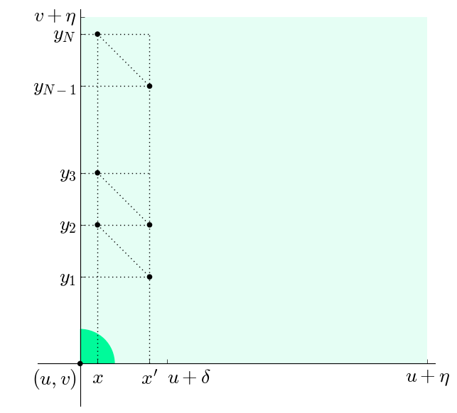
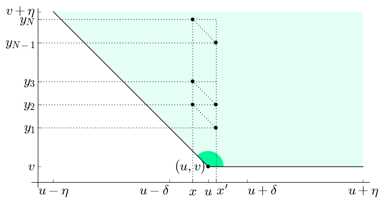
Case 1 (right-angle corner, first quadrant, Figure 3 left): Then $C_{\eta}=[u,u+\eta]\times[v,v+\eta]\subseteq F$. Define $U:=(u,u+\delta)$, $V:=(v,v+\delta)$, and $W:=(u+v,\allowbreak u+v+\delta)$.

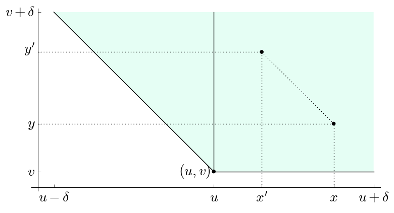
Case 2 (obtuse-angle corner, Figure 3 bottom): Then the quadrilateral $C_{\eta}=\operatorname{conv}\Bigl{(}\binom{u}{v},\binom{u-\eta}{v+\eta},\allowbreak\binom{u+\eta}{v+\eta},\binom{u+\eta}{v}\Bigr{)}$ is contained in $F$. Define $U:=(u-\delta,u+\delta)$, $V:=(v,v+\delta)$, and $W:=(u+v,\allowbreak u+v+\delta)$.

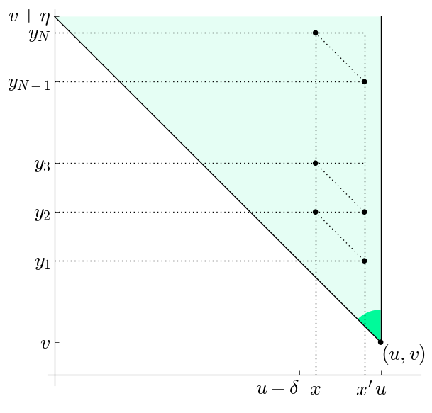
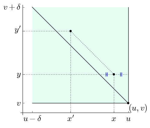
Case 3a (sharp-angle corner, Figure 3 right): Then $C_{\eta}=\operatorname{conv}\left(\binom{u}{v},\binom{u-\eta}{v+\eta},\binom{u}{v+\eta}\right)$ is contained in $F$. Define $U:=(u-\delta,u)$, $V:=(v,v+\delta)$, and $W:=(u+v,u+v+\delta)$.

Case 3b (right-angle corner, second quadrant): The sharp-angle corner of Case 3a appears as a subcone. Define $U$ and $V$ as in Case 3a and $W:=(u+v-\delta/2,\allowbreak u+v+\delta/2)$.

Note that in all cases, $U$, $V$, and $W$ are sets of the form $N_{i}\cap\operatorname{int}(p_{i}(F))$ for $i=1,2,3$, respectively, as in the claim.

We now show that

for all $$x,x^{\prime}\in U=N_{1}\cap\operatorname{int}(p_{1}(F)) \left|\tilde{\pi}_{1}(x)-\tilde{\pi}_{1}(x^{\prime})\right|\leq\varepsilon<2\varepsilon$$, we have . (4)

Let $x,x^{\prime}\in U$, without loss of generality $x<x^{\prime}$. Define a sequence $y_{n}=v+\delta+(n-1)(x^{\prime}-x)$ for $1\leq n\leq N$. Note that $\left|x-u\right|\leq\delta<\eta$, $\left|x^{\prime}-u\right|\leq\delta<\eta$ and $\left|y_{n}-v\right|=\left|\delta+(n-1)(x^{\prime}-x)\right|\leq(2n-1)\delta<\eta$ for $1\leq n\leq N$. For each $n\in\{1,2,\dots,N-1\}$, since $(x,y_{n+1}),(x^{\prime},y_{n})\in\operatorname{int}(F)$, $\|(x,y_{n+1})-(u,v)\|_{\infty}<\eta$ and $\|(x^{\prime},y_{n})-(u,v)\|_{\infty}<\eta$, we have $\left|\tilde{\pi}_{1}(x)+\tilde{\pi}_{2}(y_{n+1})-\tilde{\pi}_{3}(x+y_{n+1})\right|\leq\varepsilon/4$ and $\left|\tilde{\pi}_{1}(x^{\prime})+\tilde{\pi}_{2}(y_{n})-\tilde{\pi}_{3}(x^{\prime}+y_{n})\right|\leq\varepsilon/4$. Note that $x+y_{n+1}=x^{\prime}+y_{n}$ for $n\in\{1,2,\dots,N-1\}$, so by the triangle inequality,

$$\left|\tilde{\pi}_{1}(x)-\tilde{\pi}_{1}(x^{\prime})+\tilde{\pi}_{2}(y_{n+1})-\tilde{\pi}_{2}(y_{n})\right|\leq\varepsilon/2.$$

It follows from summing over $n=1,2,\dots,N-1$ and the triangle inequality that

$$\bigl{|}(N-1)\bigl{(}\tilde{\pi}_{1}(x)-\tilde{\pi}_{1}(x^{\prime})\bigr{)}+\tilde{\pi}_{2}(y_{N})-\tilde{\pi}_{2}(y_{1})\bigr{|}\leq(N-1)\varepsilon/2.$$

Therefore,

$$\left|\tilde{\pi}_{1}(x)-\tilde{\pi}_{1}(x^{\prime})\right| \leq\left|\tilde{\pi}_{2}(y_{N})-\tilde{\pi}_{2}(y_{1})\right|/(N-1)+\varepsilon/2$$

$$\leq 2M/(N-1)+\varepsilon/2\leq\varepsilon<2\varepsilon.$$

Case 1 and Case 2

Case 3

Figure 4. Illustration of the proof of 3.1 for $V$, equation (5).

Next we show that

for all $$y,y^{\prime}\in V=N_{2}\cap\operatorname{int}(p_{2}(F)) \left|\tilde{\pi}_{2}(y)-\tilde{\pi}_{2}(y^{\prime})\right|<2\varepsilon$$, we have . (5)

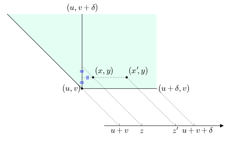
Let $y,y^{\prime}\in V$, without loss of generality $y<y^{\prime}$. In Case 1 and 2, define $x=u+(y^{\prime}-v)$; in Case 3a and 3b, define $x=u-(y-v)/2$. Let $x^{\prime}=x+y-y^{\prime}$. See Figure 4. Then $x,x^{\prime}\in U$, and hence $|\tilde{\pi}_{1}(x)-\tilde{\pi}_{1}(x^{\prime})|\leq\varepsilon$. We have $|\Delta\tilde{\pi}(x,y)|<\varepsilon/4$ and $|\Delta\tilde{\pi}(x^{\prime},y^{\prime})|<\varepsilon/4$. Then

$$\left|\tilde{\pi}_{2}(y)-\tilde{\pi}_{2}(y^{\prime})\right| =\left|\Delta\tilde{\pi}(x,y)-\Delta\tilde{\pi}(x^{\prime},y^{\prime})-(\tilde{\pi}_{1}(x)-\tilde{\pi}_{1}(x^{\prime}))\right|$$

$$\leq\varepsilon/4+\varepsilon/4+\varepsilon<2\varepsilon.$$

Case 1 and Case 2

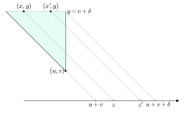
Case 3a

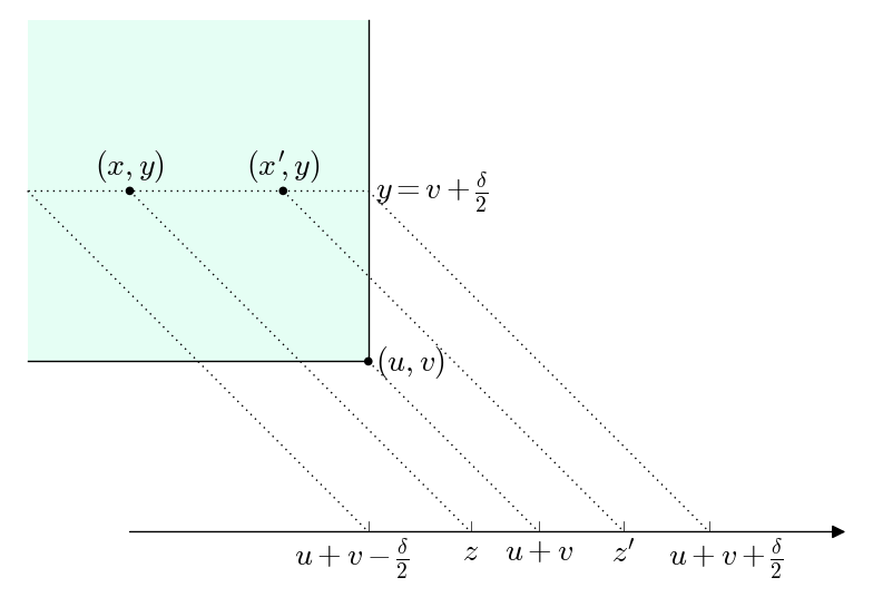
Case 3b

Figure 5. Illustration of the proof of 3.1 for $W$, equation (6).

Finally, we show that

for all $$z,z^{\prime}\in W=N_{3}\cap\operatorname{int}(p_{3}(F)) \left|\tilde{\pi}_{3}(z)-\tilde{\pi}_{3}(z^{\prime})\right|<2\varepsilon$$, we have . (6)

Let $z,z^{\prime}\in W$, without loss of generality $z<z^{\prime}$. In Case 1 and 2, define $y=v+(z-(u+v))/2$; in Case 3a, $y=v+\delta$; and in Case 3b, $y=v+\delta/2$. Let $y^{\prime}=y$. Define $x=z-y$ and $x^{\prime}=z^{\prime}-y^{\prime}$. See Figure 5. Then $x,x^{\prime}\in U$, and hence $|\tilde{\pi}_{1}(x)-\tilde{\pi}_{1}(x^{\prime})|\leq\varepsilon$. Since $(x,y),(x^{\prime},y^{\prime})\in\operatorname{int}(F)$ and $y-v=y^{\prime}-v<\eta$, we have $|\Delta\tilde{\pi}(x,y)|<\varepsilon/4$ and $|\Delta\tilde{\pi}(x^{\prime},y^{\prime})|<\varepsilon/4$. Then

$$\left|\tilde{\pi}_{3}(z)-\tilde{\pi}_{3}(z^{\prime})\right| =\left|-\Delta\tilde{\pi}(x,y)+\Delta\tilde{\pi}(x^{\prime},y^{\prime})+(\tilde{\pi}_{1}(x)-\tilde{\pi}_{1}(x^{\prime}))\right|$$

$$\leq\varepsilon/4+\varepsilon/4+\varepsilon<2\varepsilon.$$

Now we consider the tangent cones that arise when $(u,v)$ is not a vertex of $F$. Then by transformation using the same mappings, one can assume that the tangent cone $C$ is one of the following three cases:

Case 4 (upper halfplane, $y\geq v$): The obtuse-angle corner of Case 2 above is a subcone of the tangent cone. Thus, (4) and (5) hold for $U:=(u-\delta,u+\delta)$ and $V:=(v,v+\delta)$ by the same proofs. Also the 2nd quadrant of Case 3b appears as a subcone of $C$. Thus, (6) holds for $W:=(u+v-\delta/2,u+v+\delta/2)$ by the same proof. Note that $U$, $V$, and $W$ are sets of the form $N_{i}\cap\operatorname{int}(p_{i}(F))$ for $i=1,2,3$, respectively.

Case 5 (upper-right halfplane, $x+y\geq u+v$): Again the obtuse-angle corner of Case 2 above is a subset of the tangent cone. Thus, (4) and (6) hold for $U:=(u-\delta,u+\delta)$ and $W:=(u+v,u+v+\delta)$ by the same proofs. By using the transformation $(x,y)\mapsto(y,x)$ and applying the proof of (4) for Case 2 again, we also get (5) for $V:=(v-\delta,v+\delta)$. Again $U$, $V$, and $W$ are sets of the form $N_{i}\cap\operatorname{int}(p_{i}(F))$ for $i=1,2,3$, respectively.

Case 6 (entire plane). Applying Case 4, we get (4) and (5) for $U:=(u-\delta,u+\delta)$ and $W:=(u+v-\delta/2,u+v+\delta/2)$. Applying Case 4 using the transformation $(x,y)\mapsto(y,x)$, we get (5) for $V:=(v-\delta,v+\delta)$. Again $U$, $V$, and $W$ are sets of the form $N_{i}\cap\operatorname{int}(p_{i}(F))$ for $i=1,2,3$, respectively. ∎

Now we prove the theorem.

Proof of Theorem 3.1.

Let $F$ be a two-dimensional face of $\Delta\mathcal{P}$. Let $(u,v)\in F$ such that $\Delta\pi_{F}(u,v)=0$. By 2.0, $\Delta\pi_{F}(u,v)=0$ implies that

$$\Delta\tilde{\pi}_{F}(u,v)=\lim_{\begin{subarray}{c}(x,y)\to(u,v)\\ (x,y)\in\operatorname{int}(F)\end{subarray}}{\tilde{\pi}(x)+\tilde{\pi}(y)-\tilde{\pi}(x+y)}=0.$$

Because minimal valid functions take values in $[0,1]$, the effective perturbation $\tilde{\pi}$ is bounded. Thus, we can apply 3.1 to $\tilde{\pi}_{1}=\tilde{\pi}_{2}=\tilde{\pi}_{3}=\tilde{\pi}$, which gives the existence of the limits. ∎

As a consequence we obtain the following theorem regarding additive edges. It is a common generalization of [3, Lemma 4.5] by removing the assumption that all the breakpoints of $\pi$ are rational numbers; and of [15, Theorem 6.3] by removing the assumption of one-sided continuity.

Theorem 3.2.

Let $\pi$ be a minimal function that is piecewise linear over $\mathcal{P}$. Let $F$ be a one-dimensional additive face (edge) of $\Delta\mathcal{P}$. Let $\{i,j\}\subset\{1,2,3\}$ such that $p_{i}(F)$ and $p_{j}(F)$ are proper intervals. Let $E\subseteq F$ be a sub-interval. For $\theta=\pi$ or $\theta=\tilde{\pi}\in\tilde{\Pi}^{\pi}(\mathbb{R},\mathbb{Z})$, if $\theta$ is affine in $I=\operatorname{int}(p_{i}(E))$, then $\theta$ is affine in $I^{\prime}=\operatorname{int}(p_{j}(E))$ as well with the same slope.

Proof.

The proof is identical to the one of [15, Theorem 6.3], replacing the use of [15, Corollary 6.5] regarding the existence of limits by our Theorem 3.1. ∎

In the situation of the theorem, the two proper intervals $p_{i}(E)$ and $p_{j}(E)$ are said to be connected through a translation (when $F$ is a vertical or horizontal edge) or through a reflection (when $F$ is a diagonal edge). An interval $I^{\prime}$ that is connected to a covered interval $I$ is said to be (indirectly) covered and in the same connected covered component as $I$.

4. An algorithm for a restricted class of locally quasimicroperiodic perturbations

In the following, consider a finitely generated additive subgroup $T$ of the real numbers, $T=\langle t_{1},t_{2},\dots,t_{n}\rangle_{\mathbb{Z}}$, that is dense in $\mathbb{R}$.

Definition 4.0.

We define a restricted class of locally quasimicroperiodic functions as follows. Let $\bar{B}$ be a finite set of breakpoints in $[0,1]$. Consider a (perturbation) function written as $\bar{\pi}=\bar{\pi}^{\mathrm{pwl}}+\bar{\pi}^{\mathrm{micro}}$ that is periodic modulo $\mathbb{Z}$, where $\bar{\pi}^{\mathrm{pwl}}$ is (possibly discontinuous) piecewise linear over $\mathcal{P}_{\bar{B}}$, and $\bar{\pi}^{\mathrm{micro}}$ is a locally microperiodic function satisfying that

1. $\bar{\pi}^{\mathrm{micro}}(x)=0$ on any breakpoint $x\in\bar{B}$.

2. For a closed interval $I$ in $\mathcal{P}_{\bar{B}}$, $\bar{\pi}^{\mathrm{micro}}$ restricted to $\operatorname{int}(I)$ is defined as

   $$\bar{\pi}^{\mathrm{micro}}_{I}(x)=\begin{cases}c_{1}^{I}&\text{if }x\in b_{1}^{I}+T;\\ &\vdots\\ c_{m_{I}}^{I}&\text{if }x\in b_{m_{I}}^{I}+T;\\ 0&\text{otherwise},\end{cases}$$

   where $m_{I}\in\mathbb{Z}_{+}$.

(Thus, the function deviates from the piecewise linear function $\bar{\pi}^{\mathrm{pwl}}$ only on finitely many of the infinitely many additive cosets. This restriction is in place to enable computations with this class of functions.) We assume that $c^{I}_{i}\neq 0$ and $b^{I}_{i}-b^{I}_{j}\not\in T$ for $i,j\in\{1,\dots,m_{I}\},i\neq j$. If $m_{I}=0$, then $\bar{\pi}^{\mathrm{micro}}\equiv 0$ on $I$, and so $\bar{\pi}$ is linear on $\operatorname{int}(I)$. If $m_{I}>0$, we say that $\bar{\pi}^{\mathrm{micro}}$ is locally microperiodic, or, more precisely, microperiodic on the open interval $\operatorname{int}(I)$. Since $\bar{\pi}$, restricted to $\operatorname{int}(I)$, differs from $\bar{\pi}^{\mathrm{micro}}$ by a linear function, we say that it is quasimicroperiodic on $\operatorname{int}(I)$.

The perturbation function $\bar{\pi}$ that we will discuss in section 5 belongs to this restricted class.

We now consider the following algorithmic problem.

Problem 4.0.

Given (i) a minimal valid function $\pi$ that is piecewise linear over $\mathcal{P}_{B}$, (ii) a restricted locally quasimicroperiodic function $\bar{\pi}$ over $\mathcal{P}_{\bar{B}}$, determine whether $\bar{\pi}$ is an effective perturbation function for $\pi$, i.e., $\bar{\pi}\in\tilde{\Pi}^{\pi}(\mathbb{R},\mathbb{Z})$, and if yes, find an $\varepsilon>0$ such that $\pi\pm\varepsilon\bar{\pi}$ are minimal valid functions.

(By taking the union of the breakpoints and thus defining a common refinement of the complexes $\mathcal{P}_{B}$ and $\mathcal{P}_{\bar{B}}$, we can assume that $\mathcal{P}_{B}=\mathcal{P}_{\bar{B}}$.)

Consider the two-dimensional polyhedral complex $\Delta\mathcal{P}_{B}$ and its faces $F$ introduced in section 2. Theorem 4.1 below solves the decision problem of 4.0. Its proof explains how to find $\varepsilon$.

Theorem 4.1.

Let $\pi$ and $\bar{\pi}$ be as above, with $\bar{\pi}(0)=\bar{\pi}(f)=0$. The perturbation $\bar{\pi}\in\tilde{\Pi}^{\pi}(\mathbb{R},\mathbb{Z})$ if and only if

1. for any face $F$ of $\Delta\mathcal{P}_{B}$ and $(u,v)\in F$ satisfying $\Delta\pi_{F}(u,v)=0$, we have $\Delta\bar{\pi}_{F}(u,v)=0$; and

2. for any face $F$ of $\Delta\mathcal{P}_{B}$ of positive dimension such that there exists $(u,v)\in F$ satisfying $\Delta\pi_{F}(u,v)=0$, we have $\Delta\bar{\pi}^{\mathrm{micro}}_{F}(x,y)=0$ for all $(x,y)\in F$.

Proof for the $\Rightarrow$ direction:.

Assume $\bar{\pi}\in\tilde{\Pi}^{\pi}(\mathbb{R},\mathbb{Z})$. Let $\varepsilon>0$ such that $\pi+\varepsilon\bar{\pi}$ and $\pi-\varepsilon\bar{\pi}$ are minimal valid functions. Let $F$ be a face of $\Delta\mathcal{P}_{B}$ and let $(u,v)\in F$ satisfying $\Delta\pi_{F}(u,v)=0$. By 2.0, we have $\Delta\bar{\pi}_{F}(u,v)=0$. It remains to prove the second necessary condition when $F$ is not a vertex (zero-dimensional face) of $\Delta\mathcal{P}_{B}$.

Case 1: Assume that $F$ is a two-dimensional face of $\Delta\mathcal{P}_{B}$. The projections $p_{i}(F)$ ($i\in\{1,2,3\}$) are proper intervals. Assume that $p_{1}(F)\subseteq I$, $p_{2}(F)\subseteq J$, and $p_{3}(F)\subseteq K$, where $I,J,K\in\mathcal{P}_{B}$. By Theorem 3.1, the limits $\lim_{t\to p_{i}(u,v),\;t\in\operatorname{int}(p_{i}(F))}\bar{\pi}(t)$ exist. Hence, from the definitions of $\bar{\pi}^{\mathrm{micro}}_{I},\bar{\pi}^{\mathrm{micro}}_{J}$, and $\bar{\pi}^{\mathrm{micro}}_{K}$, we know that $m_{I}=m_{J}=m_{K}=0$. Then $\bar{\pi}^{\mathrm{micro}}(x)=0$ for $x\in I$, $x\in J$, or $x\in K$, which implies that $\Delta\bar{\pi}^{\mathrm{micro}}_{F}(x,y)=0$ for any $(x,y)\in F$.

Case 2: Assume that $F$ is a one-dimensional face of $\Delta\mathcal{P}_{B}$. Without loss of generality, we may assume that $F$ is a horizontal edge, i.e., $p_{1}(F)$ and $p_{3}(F)$ are closed intervals and $p_{2}(F)$ is a singleton. Let $I,J,K\in\mathcal{P}_{B}$ such that $p_{1}(F)\subseteq I$, $p_{3}(F)\subseteq K$ and $J=p_{2}(F)=\{v\}$. By hypothesis, $(u,v)\in F$, so $u\in p_{1}(F)\subseteq I$ and $u+v\in p_{3}(F)\subseteq K$.

Since the function $x\mapsto\Delta\pi_{F}(x,v)$ is affine linear over $p_{1}(F)$, there exists a constant $\alpha>0$ such that $\Delta\pi_{F}(x,v)\leq\Delta\pi_{F}(u,v)+\alpha\left|x-u\right|$ for all $x\in p_{1}(F)$. Let $x\in p_{1}(F)$. By the hypothesis $\Delta\pi_{F}(u,v)=0$, we have $\Delta\pi_{F}(x,v)\leq\alpha\left|x-u\right|$. It follows from the subadditivity of $\pi\pm\varepsilon\bar{\pi}$ that

$$\left|\Delta\bar{\pi}_{F}(x,v)\right|\leq\frac{1}{\varepsilon}\Delta\pi_{F}(x,v)\leq\frac{\alpha}{\varepsilon}\left|x-u\right|.$$

Therefore, the function $\Delta\bar{\pi}_{F}(\cdot,v)\colon p_{1}(F)\to\mathbb{R}$ is continuous at $u$, with $\Delta\bar{\pi}_{F}(u,v)=0$.

Let $x\in\operatorname{int}(p_{1}(F))\subseteq\operatorname{int}(I)$, then $x+v\in\operatorname{int}(p_{3}(F))\subseteq\operatorname{int}(K)$. We can write $\bar{\pi}^{\mathrm{micro}}(x)$ and $\bar{\pi}^{\mathrm{micro}}(x+v)$ explicitly.

$$\bar{\pi}^{\mathrm{micro}}(x)=\bar{\pi}^{\mathrm{micro}}_{I}(x)=\begin{cases}c_{i}^{I}&\text{if }x\in b_{i}^{I}+T,\;i\in\{1,\dots,m_{I}\};\\ 0&\text{otherwise},\end{cases}$$

$$\bar{\pi}^{\mathrm{micro}}(x+v)=\bar{\pi}^{\mathrm{micro}}_{K}(x+v)=\begin{cases}c_{k}^{K}&\text{if }x+v\in b_{k}^{K}+T,\;k\in\{1,\dots,m_{K}\};\\ 0&\text{otherwise}.\end{cases}$$

We also know that $\bar{\pi}^{\mathrm{micro}}(v)=0$ since $v$ is a breakpoint. Thus for $x\in\operatorname{int}(p_{1}(F))$, we have that

$$\Delta\bar{\pi}^{\mathrm{micro}}_{F}(x,v)=\Delta\bar{\pi}^{\mathrm{micro}}(x,v)=\bar{\pi}^{\mathrm{micro}}(x)-\bar{\pi}^{\mathrm{micro}}(x+v).$$ (7)

Pick a constant $b$ such that $\forall i\in\{1,\dots,m_{I}\}$, $b\not\equiv b^{I}_{i}\pmod{T}$ and $\forall k\in\{1,\dots,m_{K}\}$, $b+v\not\equiv b^{K}_{k}\pmod{T}.$ Consider a sequence $\{u_{j}\}_{j\in\mathbb{N}}$ that converges to $u$ with $u_{j}\in\operatorname{int}(p_{1}(F))$, $u_{j}\equiv b\pmod{T}$ for each $j$. The sequence $\{u_{j}\}$ exists, since $T$ is dense in $\mathbb{R}$. We have $\bar{\pi}^{\mathrm{micro}}(u_{j})=\bar{\pi}^{\mathrm{micro}}_{I}(u_{j})=0$ and $\bar{\pi}^{\mathrm{micro}}(u_{j}+v)=\bar{\pi}^{\mathrm{micro}}_{K}(u_{j}+v)=0.$ We know that $\Delta\bar{\pi}^{\mathrm{pwl}}_{F}(u_{j},v)=\Delta\bar{\pi}_{F}(u_{j},v)-\Delta\bar{\pi}^{\mathrm{micro}}_{F}(u_{j},v)$ and by (7), $\Delta\bar{\pi}^{\mathrm{micro}}_{F}(u_{j},v)=\bar{\pi}^{\mathrm{micro}}(u_{j})-\bar{\pi}^{\mathrm{micro}}\allowbreak(u_{j}+v)=0.$ Therefore, $\Delta\bar{\pi}^{\mathrm{pwl}}_{F}(u_{j},v)=\Delta\bar{\pi}_{F}(u_{j},v).$ Since $\{u_{j}\}_{j\in\mathbb{N}}$ converges to $u$, and the functions $\Delta\bar{\pi}^{\mathrm{pwl}}_{F}(\cdot,v)\colon p_{1}(F)\to\mathbb{R}$ and $\Delta\bar{\pi}_{F}(\cdot,v)\colon p_{1}(F)\to\mathbb{R}$ are continuous at $u$, by letting $j\to\infty$ in the equation above, we obtain that $\Delta\bar{\pi}^{\mathrm{pwl}}_{F}(u,v)=\Delta\bar{\pi}_{F}(u,v)=0.$

Suppose there exists $x\in\operatorname{int}(p_{1}(F))$ such that $\Delta\bar{\pi}^{\mathrm{micro}}_{F}(x,v)\neq 0$. Since $T$ is dense in $\mathbb{R}$, we can find a sequence $\{u_{j}\}_{j\in\mathbb{N}}$ converging to $u$, with $u_{j}\in\operatorname{int}(p_{1}(F))$, $u_{j}\equiv x\pmod{T}$. It follows from $\Delta\bar{\pi}^{\mathrm{micro}}_{F}(u_{j},v)=\Delta\bar{\pi}_{F}(u_{j},v)-\Delta\bar{\pi}^{\mathrm{pwl}}_{F}(u_{j},v)$ and $\Delta\bar{\pi}^{\mathrm{micro}}_{F}(u_{j},v)=\bar{\pi}^{\mathrm{micro}}(u_{j})-\bar{\pi}^{\mathrm{micro}}(u_{j}+v)=\bar{\pi}^{\mathrm{micro}}(x)-\bar{\pi}^{\mathrm{micro}}(x+v)=\Delta\bar{\pi}^{\mathrm{micro}}_{F}(x,v)$ that $\Delta\bar{\pi}_{F}(u_{j},v)-\Delta\bar{\pi}^{\mathrm{pwl}}_{F}(u_{j},v)=\Delta\bar{\pi}^{\mathrm{micro}}_{F}(x,v).$ By letting $j\to\infty$ in the above equation, we have a contradiction:

$$0=\Delta\bar{\pi}_{F}(u,v)-\Delta\bar{\pi}^{\mathrm{pwl}}_{F}(u,v)=\Delta\bar{\pi}^{\mathrm{micro}}_{F}(x,v)\neq 0.$$

Therefore, $\Delta\bar{\pi}^{\mathrm{micro}}_{F}(x,v)=0$ for all $x\in\operatorname{int}(p_{1}(F))$. The constant $\Delta\bar{\pi}^{\mathrm{micro}}_{F}(x,v)=0$ extends to the endpoints of $p_{1}(F)$. We obtain that the statement holds for all $x\in p_{1}(F)$. This concludes the proof of the $\Rightarrow$ direction. ∎

Proof for the $\Leftarrow$ direction:.

Let $\pi$ and $\bar{\pi}=\bar{\pi}^{\mathrm{pwl}}+\bar{\pi}^{\mathrm{micro}}$ be given. Assume that conditions (1) and (2) are satisfied. We want to find $\varepsilon>0$ such that $\pi^{+}=\pi+\varepsilon\bar{\pi}$ and $\pi^{-}=\pi-\varepsilon\bar{\pi}$ are both minimal valid functions. Define

$$m:=\min\{\,\Delta\pi_{F}(x,y)\mid{} (x,y)\in\operatorname{vert}(\Delta\mathcal{P}_{B}),\,F\text{ is a face of }\Delta\mathcal{P}_{B}$$

$$\text{ such that }(x,y)\in F\text{ and }\Delta\pi_{F}(x,y)\neq 0\,\};$$

$$M:=\sup_{(x,y)\in\mathbb{R}^{2}}\left|\Delta\bar{\pi}(x,y)\right|.$$

Note that $M$ is well defined since $\bar{\pi}$ is bounded. If $M=0$, for any $\varepsilon>0$, $\pi^{+}$ and $\pi^{-}$ are subadditive. In the following, we assume $M>0$. Define $\varepsilon=\frac{m}{M}.$ We also have $m>0$, since $\pi$ is subadditive and $\Delta\pi$ is non-zero somewhere. Thus, $\varepsilon>0$.

We claim that $\pi^{+}$ and $\pi^{-}$ are subadditive. Let $F$ be a face of $\Delta\mathcal{P}_{B}$ and let $(x,y)\in F$. We need to show that $\Delta\pi_{F}^{\pm}(x,y)\geq 0$. Let $S=\{\,(u,v)\in F\mid\Delta\pi_{F}(u,v)=0\,\}$. If $S=\emptyset$, then $\Delta\pi_{F}(u,v)\geq m$ for any $(u,v)\in\operatorname{vert}(F)$. Since $\Delta\pi_{F}$ is affine over $F$, we have that $\Delta\pi_{F}(x,y)\geq m$. Hence,

$$\Delta\pi_{F}^{\pm}(x,y) =\Delta\pi_{F}(x,y)\pm\varepsilon\Delta\bar{\pi}_{F}(x,y)$$ (8)

$$\geq\Delta\pi_{F}(x,y)-\varepsilon\left|\Delta\bar{\pi}_{F}(x,y)\right|\geq m-\frac{m}{M}M=0.$$

If $S\neq\emptyset$ and $F$ is a zero-dimensional face. Then $\Delta\pi_{F}(x,y)=0$, and $\Delta\bar{\pi}_{F}(x,y)=0$ by condition (1). We have that $\Delta\pi_{F}^{\pm}(x,y)=0$. Now assume that $S\neq\emptyset$ and that the face $F$ has positive dimension. By condition (2), we have that $\Delta\bar{\pi}_{F}\equiv\Delta\bar{\pi}^{\mathrm{pwl}}_{F}$ on $F$. Therefore, $\Delta\pi_{F}^{\pm}$ is affine on $F$. For any vertex $(u,v)$ of $F$, if $(u,v)\not\in S$, then $\Delta\pi_{F}(u,v)\geq m$ and thus $\Delta\pi_{F}^{\pm}(u,v)\geq 0$ by (8); if $(u,v)\in S$, then $\Delta\bar{\pi}_{F}(u,v)=\Delta\pi_{F}(u,v)=0$ by condition (1), hence $\Delta\pi_{F}^{\pm}(u,v)=0$. Since $\Delta\pi_{F}^{\pm}$ is affine on $F$ and $(x,y)\in F$, we obtain that $\Delta\pi_{F}^{\pm}(x,y)\geq 0$.

We showed that $\pi^{\pm}$ are subadditive. It is clear that $\pi^{\pm}(0)=0$ and $\pi^{\pm}(f)=1$. Let $x\in\mathbb{R}$. Since $\Delta\pi(x,f-x)=0$, condition (1) implies that $\Delta\bar{\pi}(x,f-x)=0$. We have $\bar{\pi}(x)+\bar{\pi}(f-x)=\bar{\pi}(f)=0$, and thus the symmetry condition $\pi^{\pm}(x)+\pi^{\pm}(f-x)=\pi(x)+\pi(f-x)=1$ is satisfied. We know that $\pi$ and $\bar{\pi}$ are bounded functions, thus $\pi^{\pm}$ are also bounded. Suppose that $\pi^{+}(x)<0$ for some $x\in\mathbb{R}$. Then it follows from the subadditivity that $\pi^{+}(nx)\leq n\pi^{+}(x)$ for any $n\in\mathbb{Z}_{+}$, which contradicts the fact that $\pi^{+}$ is bounded. We obtain that the functions $\pi^{\pm}$ are non-negative.

Therefore, $\pi^{\pm}$ are minimal valid functions. Thus $\bar{\pi}\in\tilde{\Pi}^{\pi}(\mathbb{R},\mathbb{Z})$. ∎

Remark 4.1 (Implementation details).

Give functions $\pi$ and $\bar{\pi}$, face $F\in\Delta\mathcal{P}_{B}$, and $(u,v)\in F$ satisfying $\Delta\pi_{F}(u,v)=0$. Depending on the dimension of the face $F$, the conditions (1) and (2) of Theorem 4.1 for having $\varepsilon>0$ are equivalent to the following finitely checkable conditions.

Case 0: $F$ is a vertex (0-dimensional face) of $\Delta\mathcal{P}_{B}$. We just check if $\bar{\pi}(u)+\bar{\pi}(v)=\bar{\pi}(u+v)$.

Case 1: $F$ is a one-dimensional face of $\Delta\mathcal{P}_{B}$. Here we consider the case that $F$ is a horizontal edge, $p_{1}(F)\subseteq I$ and $p_{3}(F)\subseteq K$ are closed intervals in $\mathcal{P}_{B}$ and $J=p_{2}(F)=\{v\}$ is a singleton in $\mathcal{P}_{B}$. The other cases are similar. We need to check

1. $\bar{\pi}^{\mathrm{pwl}}_{I}(u)+\bar{\pi}^{\mathrm{pwl}}(v)=\bar{\pi}^{\mathrm{pwl}}_{K}(u+v)$ and

2. $\bar{\pi}^{\mathrm{micro}}_{I}(x)=\bar{\pi}^{\mathrm{micro}}_{K}(x+v)$ for $x\in\operatorname{int}(p_{1}(F))$.

The latter condition is equivalent to

1. for $i\in\{1,\dots,m_{I}\}$, there is $k\in\{1,\dots,m_{K}\}$ such that $b^{I}_{i}+v-b^{K}_{k}\in T$ and $c^{I}_{i}=c^{K}_{k}$; and

2. for $k\in\{1,\dots,m_{K}\}$, there is $i\in\{1,\dots,m_{I}\}$ such that $b^{I}_{i}+v-b^{K}_{k}\in T$ and $c^{I}_{i}=c^{K}_{k}$.

Note that it suffices to consider the vertices $(u,v)$ of $F$, since $\Delta\pi_{F}(u,v)=0$ for some $(u,v)\in\operatorname{int}(F)$ implies that the same holds for vertices.

Case 2: $F$ is a two-dimensional face of $\Delta\mathcal{P}_{B}$. Assume that $p_{1}(F)\subseteq I,p_{2}(F)\subseteq J$ and $p_{3}(F)\subseteq K$, where $I,J,K\in\mathcal{P}_{B}$. The program checks if $\bar{\pi}^{\mathrm{pwl}}_{I}(u)+\bar{\pi}^{\mathrm{pwl}}_{J}(v)=\bar{\pi}^{\mathrm{pwl}}_{K}(u+v)$, and $\bar{\pi}^{\mathrm{micro}}_{I}=\bar{\pi}^{\mathrm{micro}}_{J}=\bar{\pi}^{\mathrm{micro}}_{K}\equiv 0$, i.e., $m_{I}=m_{J}=m_{K}=0$. In this case again, it suffices to consider the vertices $(u,v)$ of $F$ satisfying $\Delta\pi_{F}(u,v)=0$.

Remark 4.1.

Theorem 4.1 generalizes to a more general class of functions, in which $\bar{\pi}^{\mathrm{pwl}}$ is only required to be Lipschitz continuous (but not necessarily affine linear) over $\operatorname{rel\,int}(I)$ for each $I\in\mathcal{P}_{\bar{B}}$.

Remark 4.1.

Theorem 4.1 also generalizes immediately to a more general class of locally quasimicroperiodic functions, in which different dense subgroups $T_{I}$ of $\mathbb{R}$ are taken in different pieces $\bar{\pi}^{\mathrm{micro}}_{I}(x)$, such that the intersection $T_{I}\cap T_{J}$ is dense in $\mathbb{R}$ for any intervals $I,J\in\mathcal{P}_{\bar{B}}$.

Open question 4.1.

It is an open question whether the conditions (1) and (2) of Theorem 4.1 can be checked finitely for the generalized class of 4.1.

5. The example

Consider the piecewise linear function $\pi$ defined by its values and limits at its breakpoints $0=x_{0}<x_{1}<\dots<x_{17}=l=\frac{219}{800}<x_{18}=u=\frac{269}{800}<x_{19}=f-u=\frac{371}{800}<x_{20}=f-l=\frac{421}{800}<\dots<x_{37}=f=\frac{4}{5}<\dots<x_{40}=1$ in Table 1. We have made it available as kzh_minimal_has_only_crazy_perturbation_1.

Theorem 5.1.

The function $\pi$ defined in Table 1 has the following properties.

1. $\pi$ is a minimal valid function.

2. It cannot be written as a convex combination of piecewise continuous minimal valid functions. In particular, it cannot be written as a convex combination of piecewise linear minimal valid functions.

3. It is not extreme because it admits effective locally microperiodic perturbations. In particular, define a perturbation as follows.

   $$\bar{\pi}(x)=\begin{cases}1&\text{if }x\in(l,u)\text{ such that }x-l\in\langle t_{1},t_{2}\rangle_{\mathbb{Z}}\text{, or}\\ &\text{if }x\in(f-u,f-l)\text{ such that }x-f+u\in\langle t_{1},t_{2}\rangle_{\mathbb{Z}};\\ -1&\text{if }x\in(l,u)\text{ such that }x-u\in\langle t_{1},t_{2}\rangle_{\mathbb{Z}}\text{, or}\\ &\text{if }x\in(f-u,f-l)\text{ such that }x-f+l\in\langle t_{1},t_{2}\rangle_{\mathbb{Z}};\\ 0&\text{otherwise},\end{cases}$$ (9)

   where $f=\frac{4}{5}$, $l=\frac{219}{800}$, $u=\frac{269}{800}$, $t_{1}=\frac{77}{7752}\sqrt{2}$, $t_{2}=\frac{77}{2584}$; see Figure 2, magenta. Let $\varepsilon=0.0003$. Then $\pi\pm\varepsilon\bar{\pi}$ are minimal valid functions.

Table 1. The piecewise linear function kzh_minimal_has_only_crazy_perturbation_1, defined by its values and limits at the breakpoints. If a limit is omitted, it equals the value.

$\begin{array}[]{c@{\quad}*5c}\hline\cr\hline\cr i&x_{i}&\pi(x_{i}^{-})&\pi(x_{i})&\pi(x_{i}^{+})&\text{slope}\\ \hline\cr 0&0&\frac{101}{650}&0&\frac{101}{650}&\smash{\raisebox{-5.81247pt}{$c_{3}=-5$}}\\ 1&\frac{101}{5000}&\frac{707}{13000}&\frac{2727}{13000}&\frac{707}{13000}&\smash{\raisebox{-5.81247pt}{$c_{1}=\frac{35}{13}$}}\\ 2&\frac{60153}{369200}&&\frac{421071}{959920}&&\smash{\raisebox{-5.81247pt}{$c_{3}=-5$}}\\ 3&\frac{849}{5000}&\frac{4851099}{11999000}&-\frac{1925}{71994}\sqrt{2}+\frac{4851099}{11999000}&\frac{4851099}{11999000}&\smash{\raisebox{-5.81247pt}{$c_{1}=\frac{35}{13}$}}\\ 4&\frac{1925}{298129}\sqrt{2}+\frac{849}{5000}&&\frac{67375}{3875677}\sqrt{2}+\frac{4851099}{11999000}&&\smash{\raisebox{-5.81247pt}{$c_{3}=-5$}}\\ 5&\frac{77}{7752}\sqrt{2}+\frac{849}{5000}&\frac{385}{93016248}\sqrt{2}+\frac{4851099}{11999000}&\frac{2695}{100776}\sqrt{2}+\frac{4851099}{11999000}&\frac{385}{93016248}\sqrt{2}+\frac{4851099}{11999000}&\smash{\raisebox{-5.81247pt}{$c_{1}=\frac{35}{13}$}}\\ 6&\hbox to0.0pt{\hss$a_{0}={}$}\frac{19}{100}&-\frac{1925}{71994}\sqrt{2}+\frac{275183}{599950}&\frac{18196}{59995}&-\frac{1925}{71994}\sqrt{2}+\frac{275183}{599950}&\smash{\raisebox{-5.81247pt}{$c_{1}=\frac{35}{13}$}}\\ 7&\frac{77}{22152}\sqrt{2}+\frac{281986521}{1490645000}&&-\frac{385}{22152}\sqrt{2}+\frac{10467633}{22933000}&&\smash{\raisebox{-5.81247pt}{$c_{3}=-5$}}\\ 8&\frac{40294}{201875}&\frac{848837}{2099500}&\frac{795836841}{1937838500}&\frac{848837}{2099500}&\smash{\raisebox{-5.81247pt}{$c_{1}=\frac{35}{13}$}}\\ 9&\frac{36999}{184600}&&\frac{975607}{2399800}&&\smash{\raisebox{-5.81247pt}{$c_{3}=-5$}}\\ 10&\hbox to0.0pt{\hss$a_{1}={}$}\frac{77}{7752}\sqrt{2}+\frac{19}{100}&-\frac{385}{7752}\sqrt{2}+\frac{275183}{599950}&\frac{385}{93016248}\sqrt{2}+\frac{18196}{59995}&-\frac{385}{7752}\sqrt{2}+\frac{275183}{599950}&\smash{\raisebox{-5.81247pt}{$c_{3}=-5$}}\\ 11&\frac{1051}{5000}&\frac{4291761}{11999000}&-\frac{1925}{71994}\sqrt{2}+\frac{4291761}{11999000}&\frac{4291761}{11999000}&\smash{\raisebox{-5.81247pt}{$c_{1}=\frac{35}{13}$}}\\ 12&\frac{1925}{298129}\sqrt{2}+\frac{1051}{5000}&&\frac{67375}{3875677}\sqrt{2}+\frac{4291761}{11999000}&&\smash{\raisebox{-5.81247pt}{$c_{3}=-5$}}\\ 13&\hbox to0.0pt{\hss$a_{2}={}$}\frac{14199}{64600}&\frac{192500}{3875677}\sqrt{2}+\frac{240046061}{775135400}&\frac{50943}{167960}&\frac{192500}{3875677}\sqrt{2}+\frac{240046061}{775135400}&\smash{\raisebox{-5.81247pt}{$c_{3}=-5$}}\\ 14&\frac{77}{7752}\sqrt{2}+\frac{1051}{5000}&\frac{385}{93016248}\sqrt{2}+\frac{4291761}{11999000}&\frac{2695}{100776}\sqrt{2}+\frac{4291761}{11999000}&\frac{385}{93016248}\sqrt{2}+\frac{4291761}{11999000}&\smash{\raisebox{-5.81247pt}{$c_{1}=\frac{35}{13}$}}\\ 15&\frac{77}{22152}\sqrt{2}+\frac{342208579}{1490645000}&&-\frac{385}{22152}\sqrt{2}+\frac{122181831}{298129000}&&\smash{\raisebox{-5.81247pt}{$c_{3}=-5$}}\\ 16&\frac{193799}{807500}&&\frac{187742}{524875}&&\smash{\raisebox{-5.81247pt}{$c_{1}=\frac{35}{13}$}}\\ 17&\hbox to0.0pt{\hss$l=A={}$}\frac{219}{800}&&\frac{933}{2080}&\frac{51443}{147680}&\smash{\raisebox{-5.81247pt}{$c_{2}=\frac{5}{11999}$}}\\ 18&\hbox to0.0pt{\hss$u=A_{0}={}$}\frac{269}{800}&\frac{668809}{1919840}&\frac{683}{2080}&&\smash{\raisebox{-5.81247pt}{$c_{1}=\frac{35}{13}$}}\\ 19&\hbox to0.0pt{\hss$f-u={}$}\frac{371}{800}&&\frac{1397}{2080}&\frac{1251031}{1919840}&\smash{\raisebox{-5.81247pt}{$c_{2}=\frac{5}{11999}$}}\\ 20&\hbox to0.0pt{\hss$f-l={}$}\frac{421}{800}&\frac{96237}{147680}&\frac{1147}{2080}&&\smash{\raisebox{-5.81247pt}{$c_{1}=\frac{35}{13}$}}\\ 21&\frac{452201}{807500}&&\frac{337133}{524875}&&\smash{\raisebox{-5.81247pt}{$c_{3}=-5$}}\\ 22&-\frac{77}{22152}\sqrt{2}+\frac{850307421}{1490645000}&&\frac{385}{22152}\sqrt{2}+\frac{175947169}{298129000}&&\smash{\raisebox{-5.81247pt}{$c_{1}=\frac{35}{13}$}}\\ 23&-\frac{77}{7752}\sqrt{2}+\frac{2949}{5000}&-\frac{385}{93016248}\sqrt{2}+\frac{7707239}{11999000}&-\frac{2695}{100776}\sqrt{2}+\frac{7707239}{11999000}&-\frac{385}{93016248}\sqrt{2}+\frac{7707239}{11999000}&\smash{\raisebox{-5.81247pt}{$c_{3}=-5$}}\\ 24&\frac{37481}{64600}&-\frac{192500}{3875677}\sqrt{2}+\frac{535089339}{775135400}&\frac{117017}{167960}&-\frac{192500}{3875677}\sqrt{2}+\frac{535089339}{775135400}&\smash{\raisebox{-5.81247pt}{$c_{3}=-5$}}\\ 25&-\frac{1925}{298129}\sqrt{2}+\frac{2949}{5000}&&-\frac{67375}{3875677}\sqrt{2}+\frac{7707239}{11999000}&&\smash{\raisebox{-5.81247pt}{$c_{1}=\frac{35}{13}$}}\\ 26&\frac{2949}{5000}&\frac{7707239}{11999000}&\frac{1925}{71994}\sqrt{2}+\frac{7707239}{11999000}&\frac{7707239}{11999000}&\smash{\raisebox{-5.81247pt}{$c_{3}=-5$}}\\ 27&-\frac{77}{7752}\sqrt{2}+\frac{61}{100}&\frac{385}{7752}\sqrt{2}+\frac{324767}{599950}&-\frac{385}{93016248}\sqrt{2}+\frac{41799}{59995}&\frac{385}{7752}\sqrt{2}+\frac{324767}{599950}&\smash{\raisebox{-5.81247pt}{$c_{3}=-5$}}\\ 28&\frac{110681}{184600}&&\frac{1424193}{2399800}&&\smash{\raisebox{-5.81247pt}{$c_{1}=\frac{35}{13}$}}\\ 29&\frac{121206}{201875}&\frac{1250663}{2099500}&\frac{1142001659}{1937838500}&\frac{1250663}{2099500}&\smash{\raisebox{-5.81247pt}{$c_{3}=-5$}}\\ 30&-\frac{77}{22152}\sqrt{2}+\frac{910529479}{1490645000}&&\frac{385}{22152}\sqrt{2}+\frac{12465367}{22933000}&&\smash{\raisebox{-5.81247pt}{$c_{1}=\frac{35}{13}$}}\\ 31&\frac{61}{100}&\frac{1925}{71994}\sqrt{2}+\frac{324767}{599950}&\frac{41799}{59995}&\frac{1925}{71994}\sqrt{2}+\frac{324767}{599950}&\smash{\raisebox{-5.81247pt}{$c_{1}=\frac{35}{13}$}}\\ 32&-\frac{77}{7752}\sqrt{2}+\frac{3151}{5000}&-\frac{385}{93016248}\sqrt{2}+\frac{7147901}{11999000}&-\frac{2695}{100776}\sqrt{2}+\frac{7147901}{11999000}&-\frac{385}{93016248}\sqrt{2}+\frac{7147901}{11999000}&\smash{\raisebox{-5.81247pt}{$c_{3}=-5$}}\\ 33&-\frac{1925}{298129}\sqrt{2}+\frac{3151}{5000}&&-\frac{67375}{3875677}\sqrt{2}+\frac{7147901}{11999000}&&\smash{\raisebox{-5.81247pt}{$c_{1}=\frac{35}{13}$}}\\ 34&\frac{3151}{5000}&\frac{7147901}{11999000}&\frac{1925}{71994}\sqrt{2}+\frac{7147901}{11999000}&\frac{7147901}{11999000}&\smash{\raisebox{-5.81247pt}{$c_{3}=-5$}}\\ 35&\frac{235207}{369200}&&\frac{538849}{959920}&&\smash{\raisebox{-5.81247pt}{$c_{1}=\frac{35}{13}$}}\\ 36&\frac{3899}{5000}&\frac{12293}{13000}&\frac{10273}{13000}&\frac{12293}{13000}&\smash{\raisebox{-5.81247pt}{$c_{3}=-5$}}\\ 37&\hbox to0.0pt{\hss$f={}$}\frac{4}{5}&\frac{549}{650}&1&\frac{549}{650}&\smash{\raisebox{-5.81247pt}{$c_{1}=\frac{35}{13}$}}\\ 38&\frac{4101}{5000}&\frac{899}{1000}&\frac{9667}{13000}&\frac{899}{1000}&\smash{\raisebox{-5.81247pt}{$c_{3}=-5$}}\\ 39&\frac{4899}{5000}&\frac{101}{1000}&\frac{3333}{13000}&\frac{101}{1000}&\smash{\raisebox{-5.81247pt}{$c_{1}=\frac{35}{13}$}}\\ 40&1&\frac{101}{650}&0&\frac{101}{650}&\smash{\raisebox{-5.81247pt}{$$}}\\ \hline\cr\hline\cr\end{array}$

Proof.

Our proof is computer-assisted. The reader may verify it independently.

Part (i). Verifying minimality is a routine task, following the algorithm of [3, Theorem 2.5]; see also [15, section 5]. (The algorithm is equivalent to the one described, in the setting of discontinuous pseudo-periodic superadditive functions, in Richard, Li, and Miller [18, Theorem 22].) It is implemented in [13] as minimality_test.

    sage: h = kzh_minimal_has_only_crazy_perturbation_1()
    sage: minimality_test(h)
    True

We remark that the software uses exact computations only. For our example, these take place in the field $\mathbb{Q}(\sqrt{2})$; see Appendix A. The minimality test amounts to verifying subadditivity and symmetry on vertices of the complex $\Delta\mathcal{P}$. The reader is invited to inspect the complex $\Delta\mathcal{P}$ by using the optional argument show_plots=True in the call to minimality_test.

Part (ii). Suppose $\tilde{\pi}$ is a piecewise continuous perturbation such that $\pi\pm\tilde{\pi}$ are both minimal valid functions. We will prove that $\tilde{\pi}\equiv 0$.

The first step is to compute the directly and indirectly covered intervals, by applying Theorem 2.1 and Theorem 3.2 a total of 38 times to various additive faces of $\Delta\mathcal{P}$. This computation is implemented in generate_covered_components_strategically as a part of extremality_test. See Appendix C for a protocol of this computation. Again the reader is invited to use the optional argument show_plots=True to follow the steps of the proof visually. In steps $1$, $2$, $3$, and $6$, two-dimensional additive faces of $\Delta\mathcal{P}$ are considered via Theorem 2.1, so their projections are directly covered intervals. In the other steps, $4,5,7,8,\dots,38$, one-dimensional additive faces are considered via Theorem 3.2, and the indirectly covered intervals are found. As a result, all the intervals in $\mathcal{P}$, except for $(l,u)$ and $(f-u,f-l)$ are covered intervals belonging to two connected components. Thus the perturbation $\tilde{\pi}$ is affine linear with two independent slope parameters $\tilde{c}_{1}$ and $\tilde{c}_{3}$ on these intervals.

Next, we show that $\tilde{\pi}$ must be affine linear with some slope $\tilde{c}_{2}$ on the two remaining intervals $(l,u)$ and $(f-u,f-l)$ as well, where $l=x_{17}$, $u=x_{18}$ and $f=x_{37}$. We reuse a lemma regarding “reachability” that was used in [3, section 5] to establish the extremality of the bhk_irrational function. To this end, we introduce the following notation. Let $a_{0}=x_{6}=\frac{19}{100}$, $a_{1}=x_{10}=\frac{77}{7752}\sqrt{2}+\frac{19}{100}$ and $a_{2}=x_{13}=\frac{14199}{64600}$. Define $A=l$, $A_{0}=u$, $A_{1}=A_{0}+a_{0}-a_{1}$ and $A_{2}=A_{0}+a_{0}-a_{2}$. Let $t_{1}=a_{1}-a_{0}=\frac{77}{7752}\sqrt{2}$, $t_{2}=a_{2}-a_{0}=\frac{101}{5000}$. Then the numbers $a_{0},a_{1},a_{2},t_{1},t_{2},f,A,A_{0},A_{1},A_{2}\in(0,1)$ satisfy the condition (i) $t_{1},t_{2}$ are linearly independent over $\mathbb{Q}$, and also the conditions (ii) and (iii) of [3, Assumption 5.1]. Condition (i) implies that the group $\langle t_{1},t_{2}\rangle_{\mathbb{Z}}$ is dense in $\mathbb{R}$. One can verify that for all $x\in(A,A_{i})$, $\pi(a_{i})+\pi(x)=\pi(a_{i}+x)$ for $i=0,1,2$. Thus, the same additive equations hold for the perturbation $\tilde{\pi}$, i.e., for all $x\in(A,A_{i})$, $\tilde{\pi}(a_{i})+\tilde{\pi}(x)=\tilde{\pi}(a_{i}+x)$ for $i=0,1,2$. Let $\hat{x}$ be an arbitrary point in the interval $[l+t_{2},u-t_{2}]$. Define $k_{1}=\tilde{\pi}(a_{1})-\tilde{\pi}(a_{0})$ and $k_{2}=\tilde{\pi}(a_{2})-\tilde{\pi}(a_{0})$. By a generalization of [3, Lemma 5.2] (B.0), if $x\in(l,u)$ satisfies that $x-\hat{x}=\lambda_{1}t_{1}+\lambda_{2}t_{2}$ with $\lambda_{1},\lambda_{2}\in\mathbb{Z}$, then $\tilde{\pi}(x)-\tilde{\pi}(\hat{x})=\lambda_{1}k_{1}+\lambda_{2}k_{2}$. The piecewise continuous perturbation function $\tilde{\pi}$ is bounded. An arithmetic argument using continued fractions (B.0) then implies that $\frac{k_{1}}{t_{1}}=\frac{k_{2}}{t_{2}}$. Denote $s:=\frac{k_{1}}{t_{1}}=\frac{k_{2}}{t_{2}}$. Consider $x\in(l,u)$ such that $x-\hat{x}\in\langle t_{1},t_{2}\rangle_{\mathbb{Z}}$, i.e., $x-\hat{x}=\lambda_{1}t_{1}+\lambda_{2}t_{2}$ with $\lambda_{1},\lambda_{2}\in\mathbb{Z}$; then we have

$$\frac{\tilde{\pi}(x)-\tilde{\pi}(\hat{x})}{x-\hat{x}}=\frac{\lambda_{1}k_{1}+\lambda_{2}k_{2}}{\lambda_{1}t_{1}+\lambda_{2}t_{2}}=s.$$

Therefore, $\tilde{\pi}$ is affine linear with constant slope $s$ over each coset $\hat{x}+\langle t_{1},t_{2}\rangle_{\mathbb{Z}}$ within the interval $(l,u)$, for $\hat{x}\in[l+t_{2},u-t_{2}]$. Since $\langle t_{1},t_{2}\rangle_{\mathbb{Z}}$ is dense in $\mathbb{R}$ and the function $\tilde{\pi}$ is piecewise continuous on $(l,u)$, we conclude that $\tilde{\pi}$ is affine linear over the interval $(l,u)$ with slope $s$. The perturbation $\tilde{\pi}$ is also affine linear on the interval $(f-u,f-l)$ by the symmetry condition.

Now we can set up a “symbolic” piecewise linear function $\tilde{\pi}$ with 43 parameters, representing the 3 slopes of $\tilde{\pi}$ and 40 possible jump values at the breakpoints, taking the symmetry condition into consideration, as in [15, section 7] and similar to [3, Theorem 3.2, Remark 3.6]. The 43-dimensional homogeneous linear system implied by the additivity constraints has a full-rank subsystem. Hence the solution space has dimension 0. See again Appendix C for a protocol of this computation, which shows the 43 equations that give the full-rank system.

Part (iii). We use the algorithm of section 4. It is implemented as find_epsilon_for_crazy_perturbation. The function $\bar{\pi}=\textsf{cp}$ is defined in the doctests of kzh_minimal_has_only_crazy_perturbation_1.

    sage: find_epsilon_for_crazy_perturbation(h, cp)
    0.0003958663221935161?

This concludes the proof of the theorem. ∎

Appendix A Exact computations with algebraic field extensions

The software [13] is written in SageMath [19], a comprehensive Python-based open source computer algebra system. By default it works with (arbitrary-precision) rational numbers; but when parameters of a function are irrational algebraic numbers, it constructs a suitable number field, embedded into the real numbers, and makes exact computations with the elements of this number field.

These number fields are algebraic field extensions (in the case of the example function discussed in section 5, of degree $d=2$) of the field $\mathbb{Q}$ of rational numbers, in much the same way that the field $\mathbb{C}$ of complex numbers is an algebraic field extension (of degree $d=2$) of the field $\mathbb{R}$ of real numbers. Elements of the field are represented as a rational coordinate vector of dimension $d$ over the base field $\mathbb{Q}$, and all arithmetic computations are done by manipulating these vectors. The number fields can be considered either abstractly or as embedded subfields of an enclosing field. When we say that the number fields are embedded into the enclosing field of real numbers, this means in particular that they inherit the linear order from the real numbers. To decide whether $a<b$, one computes sufficiently many digits of both numbers using a rigorous version of Newton’s method; this is guaranteed to terminate because $a=b$ can be decided by just comparing the coordinate vectors.

The program [13] includes a function nice_field_values that provides convenient access to the standard facilities of SageMath that construct such an embedded number field.

Appendix B Arithmetic argument in the proof of Theorem 5.1 (ii)

Lemma B.0 (Generalization of [3, Lemma 5.2]).

Using the notations and under the conditions of [3, Assumption 5.1], suppose that for all $x\in[A,A_{i}]$, $\tilde{\pi}(a_{i})+\tilde{\pi}(x)=\tilde{\pi}(a_{i}+x)$ for $i=0,1,2$. Let $\hat{x}\in[A,A_{0}]$ such that $\hat{x}\pm t_{i}\in[A,A_{0}]$ for $i=1,2$. If $x=\hat{x}+\lambda_{1}t_{1}+\lambda_{2}t_{2}\in[A,A_{0}]$ with $\lambda_{1},\lambda_{2}\in\mathbb{Z}$, then

$$\tilde{\pi}(x)-\tilde{\pi}(\hat{x})=\lambda_{1}\left(\tilde{\pi}({a_{1}})-\tilde{\pi}({a_{0}})\right)+\lambda_{2}\left(\tilde{\pi}({a_{2}})-\tilde{\pi}({a_{0}})\right).$$

Proof.

The proof appears in [3] for the case $\hat{x}=(A+A_{0})/2$; this is called $x_{0}$ in [3]. The proof extends verbatim to general $\hat{x}$ as in our hypothesis. ∎

Lemma B.0.

Let $\theta\colon\mathbb{R}\to\mathbb{R}$ be a bounded function that is piecewise continuous on the interval $(l,u)$. Denote $\bar{x}:=\frac{l+u}{2}$. Let $t_{1},t_{2}$ be positive numbers that are linearly independent over $\mathbb{Q}$, and let $k_{1},k_{2}\in\mathbb{R}$. Assume that for any $x\in(l,u)$ such that $x-\bar{x}=\lambda_{1}t_{1}+\lambda_{2}t_{2}$ with $\lambda_{1},\lambda_{2}\in\mathbb{Z}$, we have $\theta(x)-\theta(\bar{x})=\lambda_{1}k_{1}+\lambda_{2}k_{2}$. Then, $\frac{k_{1}}{t_{1}}=\frac{k_{2}}{t_{2}}$.

Proof.

Suppose for the sake of contradiction that $k_{1}t_{2}=k_{2}t_{1}+\sigma$ where $\sigma\neq 0$. Let $U\in\mathbb{R}$ such that $|\theta(x)|\leq U$ for any $x$. Let $N$ be an integer such that $N>(|k_{2}|(u-l)/2+2Ut_{2})/|\sigma|$. Since $t_{1}$ and $t_{2}$ are linearly independent over $\mathbb{Q}$, $t_{1}/t_{2}$ is irrational. The continued fraction approximations for $t_{1}/t_{2}$ form an infinite sequence $\{p_{n}/q_{n}\}_{n\in\mathbb{N}}$ of successive convergents with the property that $|t_{1}/t_{2}-p_{n}/q_{n}|\leq 1/(q_{n}q_{n+1})$. Let $(\lambda_{1},\lambda_{2})=(q_{n},-p_{n})$ for some large enough index $n$, then $\lambda_{1},\lambda_{2}\in\mathbb{Z}$ satisfy that $\lambda_{1}>N$ and $|\lambda_{1}t_{1}+\lambda_{2}t_{2}|<(u-l)/2$. Let $x=\bar{x}+\lambda_{1}t_{1}+\lambda_{2}t_{2}$. Then $x\in(l,u)$, and hence $\theta(x)-\theta(\bar{x})=\lambda_{1}k_{1}+\lambda_{2}k_{2}$. We have on the one hand, $|\lambda_{1}k_{1}+\lambda_{2}k_{2}|\leq 2U$. On the other hand,

$$|\lambda_{1}k_{1}t_{2}+\lambda_{2}k_{2}t_{2}| =|\lambda_{1}(k_{2}t_{1}+\sigma)+\lambda_{2}k_{2}t_{2}|$$

$$=|k_{2}(\lambda_{1}t_{1}+\lambda_{2}t_{2})+\lambda_{1}\sigma|\geq\bigl{\lvert}\lvert\lambda_{1}\sigma\rvert-\lvert k_{2}(\lambda_{1}t_{1}+\lambda_{2}t_{2})\rvert\bigr{\rvert}.$$

Since $|\lambda_{1}\sigma|>N|\sigma|>|k_{2}|(u-l)/2+2Ut_{2}$ and $|\lambda_{1}t_{1}+\lambda_{2}t_{2}|<(u-l)/2$, we have $|\lambda_{1}k_{1}t_{2}+\lambda_{2}k_{2}t_{2}|>2Ut_{2}$. By dividing both sides by $t_{2}>0$, we obtain $|\lambda_{1}k_{1}+\lambda_{2}k_{2}|>2U$, a contradiction. Therefore, $k_{1}t_{2}=k_{2}t_{1}$. ∎

Appendix C Protocol of the automatic proof

The following is a protocol of the automatic extremality test implemented in [13]. The protocol provides the details for the proof of Theorem 5.1 (ii). We remark that by invoking extremality_test with the optional argument crazy_perturbations=False, the code is asked to test extremality relative to the space of piecewise continuous functions, which is why it computes True.

⬇

sage: import igp; from igp import *

INFO: Welcome to the infinite-group-relaxation-code. DON’T PANIC. See demo.sage for instructions.

sage: igp.show_values_of_fastpiecewise = False; igp.show_RNFElement_by_embedding = False

sage: igp.strategical_covered_components = True; logging.getLogger().setLevel(logging.DEBUG)

sage: h = kzh_minimal_has_only_crazy_perturbation_1()

INFO: Coerced into real number field: Real Number Field in ‘a‘ as the root of the defining polynomial y^2 - 2 near 1.414213562373095?

sage: extremality_test(h, crazy_perturbations=False)

INFO: pi(0) = 0. pi is subadditive. pi is symmetric. Thus pi is minimal.

INFO: Computing maximal additive faces… done

DEBUG: Step 1: Consider the 2d additive <Face ([101/5000, 1317379/9230000], [235207/369200, 1899/2500], [6066621/9230000, 3899/5000])>. [<Int(101/5000, 1317379/9230000)>, <Int(235207/369200, 3899/5000)>] is directly covered.

DEBUG: Step 2: Consider the 2d additive <Face ([2101/2500, 4899/5000], [2101/2500, 4899/5000], [9101/5000, 4899/2500])>. [<Int(4101/5000, 4899/5000)>] is directly covered.

DEBUG: Step 3: Consider the 2d additive <Face ([101/5000, 51/400], [269/800, 8871/20000], [7129/20000, 371/800])>. [<Int(101/5000, 51/400)>, <Int(269/800, 371/800)>] is directly covered. We obtain a new covered component [<Int(101/5000, 1317379/9230000)>, <Int(269/800, 371/800)>, <Int(235207/369200, 3899/5000)>], with overlapping components merged in.

DEBUG: Step 4: Consider the 1d additive <Face ([101/5000, 13941/258400], [14199/64600], [193799/807500, 219/800])>. [<Int(193799/807500, 219/800)>] is indirectly covered. We obtain a new covered component [<Int(101/5000, 1317379/9230000)>, <Int(193799/807500, 219/800)>, <Int(269/800, 371/800)>, <Int(235207/369200, 3899/5000)>], with overlapping components merged in.

DEBUG: Step 5: Consider the 1d additive <Face ([421/800, 452201/807500], [14199/64600], [192779/258400, 3899/5000])>. [<Int(421/800, 452201/807500)>] is indirectly covered. We obtain a new covered component [<Int(101/5000, 1317379/9230000)>, <Int(193799/807500, 219/800)>, <Int(269/800, 371/800)>, <Int(421/800, 452201/807500)>, <Int(235207/369200, 3899/5000)>], with overlapping components merged in.

DEBUG: Step 6: Consider the 2d additive <Face ([101/5000, 1317379/9230000], [101/5000, 1317379/9230000], [101/2500, 60153/369200])>. [<Int(101/5000, 60153/369200)>] is directly covered. We obtain a new covered component [<Int(101/5000, 60153/369200)>, <Int(193799/807500, 219/800)>, <Int(269/800, 371/800)>, <Int(421/800, 452201/807500)>, <Int(235207/369200, 3899/5000)>], with overlapping components merged in.

DEBUG: Step 7: Consider the 1d additive <Face ([101/5000, 101/2500], [3899/5000], [4/5, 4101/5000])>. [<Int(4/5, 4101/5000)>] is indirectly covered. We obtain a new covered component [<Int(101/5000, 60153/369200)>, <Int(193799/807500, 219/800)>, <Int(269/800, 371/800)>, <Int(421/800, 452201/807500)>, <Int(235207/369200, 3899/5000)>, <Int(4/5, 4101/5000)>], with overlapping components merged in.

DEBUG: Step 8: Consider the 1d additive <Face ([4899/5000, 1], [3899/5000], [4399/2500, 8899/5000])>. [<Int(4899/5000, 1)>] is indirectly covered. We obtain a new covered component [<Int(101/5000, 60153/369200)>, <Int(193799/807500, 219/800)>, <Int(269/800, 371/800)>, <Int(421/800, 452201/807500)>, <Int(235207/369200, 3899/5000)>, <Int(4/5, 4101/5000)>, <Int(4899/5000, 1)>], with overlapping components merged in.

DEBUG: Step 9: Consider the 1d additive <Face ([0, 101/5000], [4101/5000], [4101/5000, 2101/2500])>. [<Int(0, 101/5000)>] is indirectly covered. We obtain a new covered component [<Int(0, 101/5000)>, <Int(4101/5000, 4899/5000)>], with overlapping components merged in.

DEBUG: Step 10: Consider the 1d additive <Face ([0, 101/5000], [3899/5000], [3899/5000, 4/5])>. [<Int(3899/5000, 4/5)>] is indirectly covered. We obtain a new covered component [<Int(0, 101/5000)>, <Int(3899/5000, 4/5)>, <Int(4101/5000, 4899/5000)>], with overlapping components merged in.

DEBUG: Step 11: Consider the 1d additive <Face ([101/5000, -1925/298129*a + 58986029/1490645000], [77/7752*a + 19/100], [77/7752*a + 1051/5000, 77/22152*a + 342208579/1490645000])>. [<Int(77/7752*a + 1051/5000, 77/22152*a + 342208579/1490645000)>] is indirectly covered. We obtain a new covered component [<Int(101/5000, 60153/369200)>, <Int(77/7752*a + 1051/5000, 77/22152*a + 342208579/1490645000)>, <Int(193799/807500, 219/800)>, <Int(269/800, 371/800)>, <Int(421/800, 452201/807500)>, <Int(235207/369200, 3899/5000)>, <Int(4/5, 4101/5000)>, <Int(4899/5000, 1)>], with overlapping components merged in.

DEBUG: Step 12: Consider the 1d additive <Face ([-77/22152*a + 850307421/1490645000, -77/7752*a + 2949/5000], [77/7752*a + 19/100], [1925/298129*a + 1133529971/1490645000, 3899/5000])>. [<Int(-77/22152*a + 850307421/1490645000, -77/7752*a + 2949/5000)>] is indirectly covered. We obtain a new covered component [<Int(101/5000, 60153/369200)>, <Int(77/7752*a + 1051/5000, 77/22152*a + 342208579/1490645000)>, <Int(193799/807500, 219/800)>, <Int(269/800, 371/800)>, <Int(421/800, 452201/807500)>, <Int(-77/22152*a + 850307421/1490645000, -77/7752*a + 2949/5000)>, <Int(235207/369200, 3899/5000)>, <Int(4/5, 4101/5000)>, <Int(4899/5000, 1)>], with overlapping components merged in.

DEBUG: Step 13: Consider the 1d additive <Face ([101/5000, 1925/298129*a + 101/5000], [19/100], [1051/5000, 1925/298129*a + 1051/5000])>. [<Int(1051/5000, 1925/298129*a + 1051/5000)>] is indirectly covered. We obtain a new covered component [<Int(101/5000, 60153/369200)>, <Int(1051/5000, 1925/298129*a + 1051/5000)>, <Int(77/7752*a + 1051/5000, 77/22152*a + 342208579/1490645000)>, <Int(193799/807500, 219/800)>, <Int(269/800, 371/800)>, <Int(421/800, 452201/807500)>, <Int(-77/22152*a + 850307421/1490645000, -77/7752*a + 2949/5000)>, <Int(235207/369200, 3899/5000)>, <Int(4/5, 4101/5000)>, <Int(4899/5000, 1)>], with overlapping components merged in.

DEBUG: Step 14: Consider the 1d additive <Face ([-1925/298129*a + 2949/5000, 2949/5000], [19/100], [-1925/298129*a + 3899/5000, 3899/5000])>. [<Int(-1925/298129*a + 2949/5000, 2949/5000)>] is indirectly covered. We obtain a new covered component [<Int(101/5000, 60153/369200)>, <Int(1051/5000, 1925/298129*a + 1051/5000)>, <Int(77/7752*a + 1051/5000, 77/22152*a + 342208579/1490645000)>, <Int(193799/807500, 219/800)>, <Int(269/800, 371/800)>, <Int(421/800, 452201/807500)>, <Int(-77/22152*a + 850307421/1490645000, -77/7752*a + 2949/5000)>, <Int(-1925/298129*a + 2949/5000, 2949/5000)>, <Int(235207/369200, 3899/5000)>, <Int(4/5, 4101/5000)>, <Int(4899/5000, 1)>], with overlapping components merged in.

DEBUG: Step 15: Consider the 1d additive <Face ([-1925/298129*a + 3151/5000, 3151/5000], [19/100], [-1925/298129*a + 4101/5000, 4101/5000])>. [<Int(-1925/298129*a + 3151/5000, 3151/5000)>] is indirectly covered. We obtain a new covered component [<Int(101/5000, 60153/369200)>, <Int(1051/5000, 1925/298129*a + 1051/5000)>, <Int(77/7752*a + 1051/5000, 77/22152*a + 342208579/1490645000)>, <Int(193799/807500, 219/800)>, <Int(269/800, 371/800)>, <Int(421/800, 452201/807500)>, <Int(-77/22152*a + 850307421/1490645000, -77/7752*a + 2949/5000)>, <Int(-1925/298129*a + 2949/5000, 2949/5000)>, <Int(-1925/298129*a + 3151/5000, 3151/5000)>, <Int(235207/369200, 3899/5000)>, <Int(4/5, 4101/5000)>, <Int(4899/5000, 1)>], with overlapping components merged in.

DEBUG: Step 16: Consider the 1d additive <Face ([4899/5000, 1925/298129*a + 4899/5000], [19/100], [5849/5000, 1925/298129*a + 5849/5000])>. [<Int(849/5000, 1925/298129*a + 849/5000)>] is indirectly covered. We obtain a new covered component [<Int(101/5000, 60153/369200)>, <Int(849/5000, 1925/298129*a + 849/5000)>, <Int(1051/5000, 1925/298129*a + 1051/5000)>, <Int(77/7752*a + 1051/5000, 77/22152*a + 342208579/1490645000)>, <Int(193799/807500, 219/800)>, <Int(269/800, 371/800)>, <Int(421/800, 452201/807500)>, <Int(-77/22152*a + 850307421/1490645000, -77/7752*a + 2949/5000)>, <Int(-1925/298129*a + 2949/5000, 2949/5000)>, <Int(-1925/298129*a + 3151/5000, 3151/5000)>, <Int(235207/369200, 3899/5000)>, <Int(4/5, 4101/5000)>, <Int(4899/5000, 1)>], with overlapping components merged in.

DEBUG: Step 17: Consider the 1d additive <Face ([3151/5000, 235207/369200], [19/100], [4101/5000, 61071/73840])>. [<Int(3151/5000, 235207/369200)>] is indirectly covered. We obtain a new covered component [<Int(0, 101/5000)>, <Int(3151/5000, 235207/369200)>, <Int(3899/5000, 4/5)>, <Int(4101/5000, 4899/5000)>], with overlapping components merged in.

DEBUG: Step 18: Consider the 1d additive <Face ([71841/73840, 4899/5000], [19/100], [429353/369200, 5849/5000])>. [<Int(60153/369200, 849/5000)>] is indirectly covered. We obtain a new covered component [<Int(0, 101/5000)>, <Int(60153/369200, 849/5000)>, <Int(3151/5000, 235207/369200)>, <Int(3899/5000, 4/5)>, <Int(4101/5000, 4899/5000)>], with overlapping components merged in.

DEBUG: Step 19: Consider the 1d additive <Face ([77/7752*a, 101/5000], [19/100], [77/7752*a + 19/100, 1051/5000])>. [<Int(77/7752*a + 19/100, 1051/5000)>] is indirectly covered. We obtain a new covered component [<Int(0, 101/5000)>, <Int(60153/369200, 849/5000)>, <Int(77/7752*a + 19/100, 1051/5000)>, <Int(3151/5000, 235207/369200)>, <Int(3899/5000, 4/5)>, <Int(4101/5000, 4899/5000)>], with overlapping components merged in.

DEBUG: Step 20: Consider the 1d additive <Face ([2949/5000, -77/7752*a + 61/100], [19/100], [3899/5000, -77/7752*a + 4/5])>. [<Int(2949/5000, -77/7752*a + 61/100)>] is indirectly covered. We obtain a new covered component [<Int(0, 101/5000)>, <Int(60153/369200, 849/5000)>, <Int(77/7752*a + 19/100, 1051/5000)>, <Int(2949/5000, -77/7752*a + 61/100)>, <Int(3151/5000, 235207/369200)>, <Int(3899/5000, 4/5)>, <Int(4101/5000, 4899/5000)>], with overlapping components merged in.

DEBUG: Step 21: Consider the 1d additive <Face ([61/100, -77/7752*a + 3151/5000], [77/7752*a + 19/100], [77/7752*a + 4/5, 4101/5000])>. [<Int(61/100, -77/7752*a + 3151/5000)>] is indirectly covered. We obtain a new covered component [<Int(101/5000, 60153/369200)>, <Int(849/5000, 1925/298129*a + 849/5000)>, <Int(1051/5000, 1925/298129*a + 1051/5000)>, <Int(77/7752*a + 1051/5000, 77/22152*a + 342208579/1490645000)>, <Int(193799/807500, 219/800)>, <Int(269/800, 371/800)>, <Int(421/800, 452201/807500)>, <Int(-77/22152*a + 850307421/1490645000, -77/7752*a + 2949/5000)>, <Int(-1925/298129*a + 2949/5000, 2949/5000)>, <Int(61/100, -77/7752*a + 3151/5000)>, <Int(-1925/298129*a + 3151/5000, 3151/5000)>, <Int(235207/369200, 3899/5000)>, <Int(4/5, 4101/5000)>, <Int(4899/5000, 1)>], with overlapping components merged in.

DEBUG: Step 22: Consider the 1d additive <Face ([4899/5000, -77/7752*a + 1], [77/7752*a + 19/100], [77/7752*a + 5849/5000, 119/100])>. [<Int(77/7752*a + 849/5000, 19/100)>] is indirectly covered. We obtain a new covered component [<Int(101/5000, 60153/369200)>, <Int(849/5000, 1925/298129*a + 849/5000)>, <Int(77/7752*a + 849/5000, 19/100)>, <Int(1051/5000, 1925/298129*a + 1051/5000)>, <Int(77/7752*a + 1051/5000, 77/22152*a + 342208579/1490645000)>, <Int(193799/807500, 219/800)>, <Int(269/800, 371/800)>, <Int(421/800, 452201/807500)>, <Int(-77/22152*a + 850307421/1490645000, -77/7752*a + 2949/5000)>, <Int(-1925/298129*a + 2949/5000, 2949/5000)>, <Int(61/100, -77/7752*a + 3151/5000)>, <Int(-1925/298129*a + 3151/5000, 3151/5000)>, <Int(235207/369200, 3899/5000)>, <Int(4/5, 4101/5000)>, <Int(4899/5000, 1)>], with overlapping components merged in.

DEBUG: Step 23: Consider the 1d additive <Face ([77/22152*a + 22549/2307500, 101/5000], [14199/64600], [77/22152*a + 342208579/1490645000, 193799/807500])>. [<Int(77/22152*a + 342208579/1490645000, 193799/807500)>] is indirectly covered. We obtain a new covered component [<Int(0, 101/5000)>, <Int(60153/369200, 849/5000)>, <Int(77/7752*a + 19/100, 1051/5000)>, <Int(77/22152*a + 342208579/1490645000, 193799/807500)>, <Int(2949/5000, -77/7752*a + 61/100)>, <Int(3151/5000, 235207/369200)>, <Int(3899/5000, 4/5)>, <Int(4101/5000, 4899/5000)>], with overlapping components merged in.

DEBUG: Step 24: Consider the 1d additive <Face ([452201/807500, -77/22152*a + 850307421/1490645000], [14199/64600], [3899/5000, -77/22152*a + 1823451/2307500])>. [<Int(452201/807500, -77/22152*a + 850307421/1490645000)>] is indirectly covered. We obtain a new covered component [<Int(0, 101/5000)>, <Int(60153/369200, 849/5000)>, <Int(77/7752*a + 19/100, 1051/5000)>, <Int(77/22152*a + 342208579/1490645000, 193799/807500)>, <Int(452201/807500, -77/22152*a + 850307421/1490645000)>, <Int(2949/5000, -77/7752*a + 61/100)>, <Int(3151/5000, 235207/369200)>, <Int(3899/5000, 4/5)>, <Int(4101/5000, 4899/5000)>], with overlapping components merged in.

DEBUG: Step 25: Consider the 1d additive <Face ([121206/201875, -77/22152*a + 910529479/1490645000], [14199/64600], [4101/5000, -77/22152*a + 958337/1153750])>. [<Int(121206/201875, -77/22152*a + 910529479/1490645000)>] is indirectly covered. We obtain a new covered component [<Int(0, 101/5000)>, <Int(60153/369200, 849/5000)>, <Int(77/7752*a + 19/100, 1051/5000)>, <Int(77/22152*a + 342208579/1490645000, 193799/807500)>, <Int(452201/807500, -77/22152*a + 850307421/1490645000)>, <Int(2949/5000, -77/7752*a + 61/100)>, <Int(121206/201875, -77/22152*a + 910529479/1490645000)>, <Int(3151/5000, 235207/369200)>, <Int(3899/5000, 4/5)>, <Int(4101/5000, 4899/5000)>], with overlapping components merged in.

DEBUG: Step 26: Consider the 1d additive <Face ([77/22152*a + 1118413/1153750, 4899/5000], [14199/64600], [77/22152*a + 1772631521/1490645000, 242169/201875])>. [<Int(77/22152*a + 281986521/1490645000, 40294/201875)>] is indirectly covered. We obtain a new covered component [<Int(0, 101/5000)>, <Int(60153/369200, 849/5000)>, <Int(77/22152*a + 281986521/1490645000, 40294/201875)>, <Int(77/7752*a + 19/100, 1051/5000)>, <Int(77/22152*a + 342208579/1490645000, 193799/807500)>, <Int(452201/807500, -77/22152*a + 850307421/1490645000)>, <Int(2949/5000, -77/7752*a + 61/100)>, <Int(121206/201875, -77/22152*a + 910529479/1490645000)>, <Int(3151/5000, 235207/369200)>, <Int(3899/5000, 4/5)>, <Int(4101/5000, 4899/5000)>], with overlapping components merged in.

DEBUG: Step 27: Consider the 1d additive <Face ([-77/7752*a + 3151/5000, -1925/298129*a + 3151/5000], [77/7752*a + 19/100], [4101/5000, 77/22152*a + 4101/5000])>. [<Int(-77/7752*a + 3151/5000, -1925/298129*a + 3151/5000)>] is indirectly covered. We obtain a new covered component [<Int(0, 101/5000)>, <Int(60153/369200, 849/5000)>, <Int(77/22152*a + 281986521/1490645000, 40294/201875)>, <Int(77/7752*a + 19/100, 1051/5000)>, <Int(77/22152*a + 342208579/1490645000, 193799/807500)>, <Int(452201/807500, -77/22152*a + 850307421/1490645000)>, <Int(2949/5000, -77/7752*a + 61/100)>, <Int(121206/201875, -77/22152*a + 910529479/1490645000)>, <Int(-77/7752*a + 3151/5000, -1925/298129*a + 3151/5000)>, <Int(3151/5000, 235207/369200)>, <Int(3899/5000, 4/5)>, <Int(4101/5000, 4899/5000)>], with overlapping components merged in.

DEBUG: Step 28: Consider the 1d additive <Face ([-77/22152*a + 4899/5000, 4899/5000], [77/7752*a + 19/100], [1925/298129*a + 5849/5000, 77/7752*a + 5849/5000])>. [<Int(1925/298129*a + 849/5000, 77/7752*a + 849/5000)>] is indirectly covered. We obtain a new covered component [<Int(0, 101/5000)>, <Int(60153/369200, 849/5000)>, <Int(1925/298129*a + 849/5000, 77/7752*a + 849/5000)>, <Int(77/22152*a + 281986521/1490645000, 40294/201875)>, <Int(77/7752*a + 19/100, 1051/5000)>, <Int(77/22152*a + 342208579/1490645000, 193799/807500)>, <Int(452201/807500, -77/22152*a + 850307421/1490645000)>, <Int(2949/5000, -77/7752*a + 61/100)>, <Int(121206/201875, -77/22152*a + 910529479/1490645000)>, <Int(-77/7752*a + 3151/5000, -1925/298129*a + 3151/5000)>, <Int(3151/5000, 235207/369200)>, <Int(3899/5000, 4/5)>, <Int(4101/5000, 4899/5000)>], with overlapping components merged in.

DEBUG: Step 29: Consider the 1d additive <Face ([-77/7752*a + 77/2584, 101/5000], [77/7752*a + 19/100], [14199/64600, 77/7752*a + 1051/5000])>. [<Int(14199/64600, 77/7752*a + 1051/5000)>] is indirectly covered. We obtain a new covered component [<Int(0, 101/5000)>, <Int(60153/369200, 849/5000)>, <Int(1925/298129*a + 849/5000, 77/7752*a + 849/5000)>, <Int(77/22152*a + 281986521/1490645000, 40294/201875)>, <Int(77/7752*a + 19/100, 1051/5000)>, <Int(14199/64600, 77/7752*a + 1051/5000)>, <Int(77/22152*a + 342208579/1490645000, 193799/807500)>, <Int(452201/807500, -77/22152*a + 850307421/1490645000)>, <Int(2949/5000, -77/7752*a + 61/100)>, <Int(121206/201875, -77/22152*a + 910529479/1490645000)>, <Int(-77/7752*a + 3151/5000, -1925/298129*a + 3151/5000)>, <Int(3151/5000, 235207/369200)>, <Int(3899/5000, 4/5)>, <Int(4101/5000, 4899/5000)>], with overlapping components merged in.

DEBUG: Step 30: Consider the 1d additive <Face ([-77/7752*a + 2949/5000, 37481/64600], [77/7752*a + 19/100], [3899/5000, 77/7752*a + 9951/12920])>. [<Int(-77/7752*a + 2949/5000, 37481/64600)>] is indirectly covered. We obtain a new covered component [<Int(0, 101/5000)>, <Int(60153/369200, 849/5000)>, <Int(1925/298129*a + 849/5000, 77/7752*a + 849/5000)>, <Int(77/22152*a + 281986521/1490645000, 40294/201875)>, <Int(77/7752*a + 19/100, 1051/5000)>, <Int(14199/64600, 77/7752*a + 1051/5000)>, <Int(77/22152*a + 342208579/1490645000, 193799/807500)>, <Int(452201/807500, -77/22152*a + 850307421/1490645000)>, <Int(-77/7752*a + 2949/5000, 37481/64600)>, <Int(2949/5000, -77/7752*a + 61/100)>, <Int(121206/201875, -77/22152*a + 910529479/1490645000)>, <Int(-77/7752*a + 3151/5000, -1925/298129*a + 3151/5000)>, <Int(3151/5000, 235207/369200)>, <Int(3899/5000, 4/5)>, <Int(4101/5000, 4899/5000)>], with overlapping components merged in.

DEBUG: Step 31: Consider the 1d additive <Face ([101/5000, 77/22152*a + 5775/298129], [849/5000], [19/100, 77/22152*a + 281986521/1490645000])>. [<Int(19/100, 77/22152*a + 281986521/1490645000)>] is indirectly covered. We obtain a new covered component [<Int(101/5000, 60153/369200)>, <Int(849/5000, 1925/298129*a + 849/5000)>, <Int(77/7752*a + 849/5000, 19/100)>, <Int(19/100, 77/22152*a + 281986521/1490645000)>, <Int(1051/5000, 1925/298129*a + 1051/5000)>, <Int(77/7752*a + 1051/5000, 77/22152*a + 342208579/1490645000)>, <Int(193799/807500, 219/800)>, <Int(269/800, 371/800)>, <Int(421/800, 452201/807500)>, <Int(-77/22152*a + 850307421/1490645000, -77/7752*a + 2949/5000)>, <Int(-1925/298129*a + 2949/5000, 2949/5000)>, <Int(61/100, -77/7752*a + 3151/5000)>, <Int(-1925/298129*a + 3151/5000, 3151/5000)>, <Int(235207/369200, 3899/5000)>, <Int(4/5, 4101/5000)>, <Int(4899/5000, 1)>], with overlapping components merged in.

DEBUG: Step 32: Consider the 1d additive <Face ([-77/22152*a + 910529479/1490645000, 61/100], [849/5000], [-77/22152*a + 1163641/1490645, 3899/5000])>. [<Int(-77/22152*a + 910529479/1490645000, 61/100)>] is indirectly covered. We obtain a new covered component [<Int(101/5000, 60153/369200)>, <Int(849/5000, 1925/298129*a + 849/5000)>, <Int(77/7752*a + 849/5000, 19/100)>, <Int(19/100, 77/22152*a + 281986521/1490645000)>, <Int(1051/5000, 1925/298129*a + 1051/5000)>, <Int(77/7752*a + 1051/5000, 77/22152*a + 342208579/1490645000)>, <Int(193799/807500, 219/800)>, <Int(269/800, 371/800)>, <Int(421/800, 452201/807500)>, <Int(-77/22152*a + 850307421/1490645000, -77/7752*a + 2949/5000)>, <Int(-1925/298129*a + 2949/5000, 2949/5000)>, <Int(-77/22152*a + 910529479/1490645000, 61/100)>, <Int(61/100, -77/7752*a + 3151/5000)>, <Int(-1925/298129*a + 3151/5000, 3151/5000)>, <Int(235207/369200, 3899/5000)>, <Int(4/5, 4101/5000)>, <Int(4899/5000, 1)>], with overlapping components merged in.

DEBUG: Step 33: Consider the 1d additive <Face ([77/7384, 77/7752*a], [19/100], [36999/184600, 77/7752*a + 19/100])>. [<Int(36999/184600, 77/7752*a + 19/100)>] is indirectly covered. We obtain a new covered component [<Int(0, 101/5000)>, <Int(60153/369200, 849/5000)>, <Int(1925/298129*a + 849/5000, 77/7752*a + 849/5000)>, <Int(77/22152*a + 281986521/1490645000, 40294/201875)>, <Int(36999/184600, 77/7752*a + 19/100)>, <Int(77/7752*a + 19/100, 1051/5000)>, <Int(14199/64600, 77/7752*a + 1051/5000)>, <Int(77/22152*a + 342208579/1490645000, 193799/807500)>, <Int(452201/807500, -77/22152*a + 850307421/1490645000)>, <Int(-77/7752*a + 2949/5000, 37481/64600)>, <Int(2949/5000, -77/7752*a + 61/100)>, <Int(121206/201875, -77/22152*a + 910529479/1490645000)>, <Int(-77/7752*a + 3151/5000, -1925/298129*a + 3151/5000)>, <Int(3151/5000, 235207/369200)>, <Int(3899/5000, 4/5)>, <Int(4101/5000, 4899/5000)>], with overlapping components merged in.

DEBUG: Step 34: Consider the 1d additive <Face ([-77/7752*a + 61/100, 110681/184600], [19/100], [-77/7752*a + 4/5, 29151/36920])>. [<Int(-77/7752*a + 61/100, 110681/184600)>] is indirectly covered. We obtain a new covered component [<Int(0, 101/5000)>, <Int(60153/369200, 849/5000)>, <Int(1925/298129*a + 849/5000, 77/7752*a + 849/5000)>, <Int(77/22152*a + 281986521/1490645000, 40294/201875)>, <Int(36999/184600, 77/7752*a + 19/100)>, <Int(77/7752*a + 19/100, 1051/5000)>, <Int(14199/64600, 77/7752*a + 1051/5000)>, <Int(77/22152*a + 342208579/1490645000, 193799/807500)>, <Int(452201/807500, -77/22152*a + 850307421/1490645000)>, <Int(-77/7752*a + 2949/5000, 37481/64600)>, <Int(2949/5000, -77/7752*a + 61/100)>, <Int(-77/7752*a + 61/100, 110681/184600)>, <Int(121206/201875, -77/22152*a + 910529479/1490645000)>, <Int(-77/7752*a + 3151/5000, -1925/298129*a + 3151/5000)>, <Int(3151/5000, 235207/369200)>, <Int(3899/5000, 4/5)>, <Int(4101/5000, 4899/5000)>], with overlapping components merged in.

DEBUG: Step 35: Consider the 1d additive <Face ([110681/184600, 121206/201875], [14199/64600], [1221391/1490645, 4101/5000])>. [<Int(110681/184600, 121206/201875)>] is indirectly covered. We obtain a new covered component [<Int(101/5000, 60153/369200)>, <Int(849/5000, 1925/298129*a + 849/5000)>, <Int(77/7752*a + 849/5000, 19/100)>, <Int(19/100, 77/22152*a + 281986521/1490645000)>, <Int(1051/5000, 1925/298129*a + 1051/5000)>, <Int(77/7752*a + 1051/5000, 77/22152*a + 342208579/1490645000)>, <Int(193799/807500, 219/800)>, <Int(269/800, 371/800)>, <Int(421/800, 452201/807500)>, <Int(-77/22152*a + 850307421/1490645000, -77/7752*a + 2949/5000)>, <Int(-1925/298129*a + 2949/5000, 2949/5000)>, <Int(110681/184600, 121206/201875)>, <Int(-77/22152*a + 910529479/1490645000, 61/100)>, <Int(61/100, -77/7752*a + 3151/5000)>, <Int(-1925/298129*a + 3151/5000, 3151/5000)>, <Int(235207/369200, 3899/5000)>, <Int(4/5, 4101/5000)>, <Int(4899/5000, 1)>], with overlapping components merged in.

DEBUG: Step 36: Consider the 1d additive <Face ([4899/5000, 292354/298129], [14199/64600], [242169/201875, 221599/184600])>. [<Int(40294/201875, 36999/184600)>] is indirectly covered. We obtain a new covered component [<Int(101/5000, 60153/369200)>, <Int(849/5000, 1925/298129*a + 849/5000)>, <Int(77/7752*a + 849/5000, 19/100)>, <Int(19/100, 77/22152*a + 281986521/1490645000)>, <Int(40294/201875, 36999/184600)>, <Int(1051/5000, 1925/298129*a + 1051/5000)>, <Int(77/7752*a + 1051/5000, 77/22152*a + 342208579/1490645000)>, <Int(193799/807500, 219/800)>, <Int(269/800, 371/800)>, <Int(421/800, 452201/807500)>, <Int(-77/22152*a + 850307421/1490645000, -77/7752*a + 2949/5000)>, <Int(-1925/298129*a + 2949/5000, 2949/5000)>, <Int(110681/184600, 121206/201875)>, <Int(-77/22152*a + 910529479/1490645000, 61/100)>, <Int(61/100, -77/7752*a + 3151/5000)>, <Int(-1925/298129*a + 3151/5000, 3151/5000)>, <Int(235207/369200, 3899/5000)>, <Int(4/5, 4101/5000)>, <Int(4899/5000, 1)>], with overlapping components merged in.

DEBUG: Step 37: Consider the 1d additive <Face ([-77/22152*a + 101/5000, -77/7752*a + 77/2584], [77/7752*a + 19/100], [1925/298129*a + 1051/5000, 14199/64600])>. [<Int(1925/298129*a + 1051/5000, 14199/64600)>] is indirectly covered. We obtain a new covered component [<Int(0, 101/5000)>, <Int(60153/369200, 849/5000)>, <Int(1925/298129*a + 849/5000, 77/7752*a + 849/5000)>, <Int(77/22152*a + 281986521/1490645000, 40294/201875)>, <Int(36999/184600, 77/7752*a + 19/100)>, <Int(77/7752*a + 19/100, 1051/5000)>, <Int(1925/298129*a + 1051/5000, 14199/64600)>, <Int(14199/64600, 77/7752*a + 1051/5000)>, <Int(77/22152*a + 342208579/1490645000, 193799/807500)>, <Int(452201/807500, -77/22152*a + 850307421/1490645000)>, <Int(-77/7752*a + 2949/5000, 37481/64600)>, <Int(2949/5000, -77/7752*a + 61/100)>, <Int(-77/7752*a + 61/100, 110681/184600)>, <Int(121206/201875, -77/22152*a + 910529479/1490645000)>, <Int(-77/7752*a + 3151/5000, -1925/298129*a + 3151/5000)>, <Int(3151/5000, 235207/369200)>, <Int(3899/5000, 4/5)>, <Int(4101/5000, 4899/5000)>], with overlapping components merged in.

DEBUG: Step 38: Consider the 1d additive <Face ([37481/64600, -1925/298129*a + 2949/5000], [77/7752*a + 19/100], [77/7752*a + 9951/12920, 77/22152*a + 3899/5000])>. [<Int(37481/64600, -1925/298129*a + 2949/5000)>] is indirectly covered. We obtain a new covered component [<Int(0, 101/5000)>, <Int(60153/369200, 849/5000)>, <Int(1925/298129*a + 849/5000, 77/7752*a + 849/5000)>, <Int(77/22152*a + 281986521/1490645000, 40294/201875)>, <Int(36999/184600, 77/7752*a + 19/100)>, <Int(77/7752*a + 19/100, 1051/5000)>, <Int(1925/298129*a + 1051/5000, 14199/64600)>, <Int(14199/64600, 77/7752*a + 1051/5000)>, <Int(77/22152*a + 342208579/1490645000, 193799/807500)>, <Int(452201/807500, -77/22152*a + 850307421/1490645000)>, <Int(-77/7752*a + 2949/5000, 37481/64600)>, <Int(37481/64600, -1925/298129*a + 2949/5000)>, <Int(2949/5000, -77/7752*a + 61/100)>, <Int(-77/7752*a + 61/100, 110681/184600)>, <Int(121206/201875, -77/22152*a + 910529479/1490645000)>, <Int(-77/7752*a + 3151/5000, -1925/298129*a + 3151/5000)>, <Int(3151/5000, 235207/369200)>, <Int(3899/5000, 4/5)>, <Int(4101/5000, 4899/5000)>], with overlapping components merged in.

INFO: Completing 11 functional directed moves and 2 covered components…

INFO: Completing 26 functional directed moves and 2 covered components…

INFO: New dense move from strip lemma: [<Int(219/800, 269/800)>, <Int(371/800, 421/800)>]

INFO: Completing 0 functional directed moves and 3 covered components…

INFO: Completion finished. Found 0 directed moves and 3 covered components.

INFO: All intervals are covered (or connected-to-covered). 3 components.

DEBUG: The covered components are [[<Int(101/5000, 60153/369200)>, <Int(849/5000, 1925/298129*a + 849/5000)>, <Int(77/7752*a + 849/5000, 19/100)>, <Int(19/100, 77/22152*a + 281986521/1490645000)>, <Int(40294/201875, 36999/184600)>, <Int(1051/5000, 1925/298129*a + 1051/5000)>, <Int(77/7752*a + 1051/5000, 77/22152*a + 342208579/1490645000)>, <Int(193799/807500, 219/800)>, <Int(269/800, 371/800)>, <Int(421/800, 452201/807500)>, <Int(-77/22152*a + 850307421/1490645000, -77/7752*a + 2949/5000)>, <Int(-1925/298129*a + 2949/5000, 2949/5000)>, <Int(110681/184600, 121206/201875)>, <Int(-77/22152*a + 910529479/1490645000, 61/100)>, <Int(61/100, -77/7752*a + 3151/5000)>, <Int(-1925/298129*a + 3151/5000, 3151/5000)>, <Int(235207/369200, 3899/5000)>, <Int(4/5, 4101/5000)>, <Int(4899/5000, 1)>], [<Int(0, 101/5000)>, <Int(60153/369200, 849/5000)>, <Int(1925/298129*a + 849/5000, 77/7752*a + 849/5000)>, <Int(77/22152*a + 281986521/1490645000, 40294/201875)>, <Int(36999/184600, 77/7752*a + 19/100)>, <Int(77/7752*a + 19/100, 1051/5000)>, <Int(1925/298129*a + 1051/5000, 14199/64600)>, <Int(14199/64600, 77/7752*a + 1051/5000)>, <Int(77/22152*a + 342208579/1490645000, 193799/807500)>, <Int(452201/807500, -77/22152*a + 850307421/1490645000)>, <Int(-77/7752*a + 2949/5000, 37481/64600)>, <Int(37481/64600, -1925/298129*a + 2949/5000)>, <Int(2949/5000, -77/7752*a + 61/100)>, <Int(-77/7752*a + 61/100, 110681/184600)>, <Int(121206/201875, -77/22152*a + 910529479/1490645000)>, <Int(-77/7752*a + 3151/5000, -1925/298129*a + 3151/5000)>, <Int(3151/5000, 235207/369200)>, <Int(3899/5000, 4/5)>, <Int(4101/5000, 4899/5000)>], [<Int(219/800, 269/800)>, <Int(371/800, 421/800)>]].

DEBUG: Let v in R^43. The i-th entry of v represents the slope parameter on the i-th component of [[<Int(101/5000, 60153/369200)>, <Int(849/5000, 1925/298129*a + 849/5000)>, <Int(77/7752*a + 849/5000, 19/100)>, <Int(19/100, 77/22152*a + 281986521/1490645000)>, <Int(40294/201875, 36999/184600)>, <Int(1051/5000, 1925/298129*a + 1051/5000)>, <Int(77/7752*a + 1051/5000, 77/22152*a + 342208579/1490645000)>, <Int(193799/807500, 219/800)>, <Int(269/800, 371/800)>, <Int(421/800, 452201/807500)>, <Int(-77/22152*a + 850307421/1490645000, -77/7752*a + 2949/5000)>, <Int(-1925/298129*a + 2949/5000, 2949/5000)>, <Int(110681/184600, 121206/201875)>, <Int(-77/22152*a + 910529479/1490645000, 61/100)>, <Int(61/100, -77/7752*a + 3151/5000)>, <Int(-1925/298129*a + 3151/5000, 3151/5000)>, <Int(235207/369200, 3899/5000)>, <Int(4/5, 4101/5000)>, <Int(4899/5000, 1)>], [<Int(0, 101/5000)>, <Int(60153/369200, 849/5000)>, <Int(1925/298129*a + 849/5000, 77/7752*a + 849/5000)>, <Int(77/22152*a + 281986521/1490645000, 40294/201875)>, <Int(36999/184600, 77/7752*a + 19/100)>, <Int(77/7752*a + 19/100, 1051/5000)>, <Int(1925/298129*a + 1051/5000, 14199/64600)>, <Int(14199/64600, 77/7752*a + 1051/5000)>, <Int(77/22152*a + 342208579/1490645000, 193799/807500)>, <Int(452201/807500, -77/22152*a + 850307421/1490645000)>, <Int(-77/7752*a + 2949/5000, 37481/64600)>, <Int(37481/64600, -1925/298129*a + 2949/5000)>, <Int(2949/5000, -77/7752*a + 61/100)>, <Int(-77/7752*a + 61/100, 110681/184600)>, <Int(121206/201875, -77/22152*a + 910529479/1490645000)>, <Int(-77/7752*a + 3151/5000, -1925/298129*a + 3151/5000)>, <Int(3151/5000, 235207/369200)>, <Int(3899/5000, 4/5)>, <Int(4101/5000, 4899/5000)>], [<Int(219/800, 269/800)>, <Int(371/800, 421/800)>]] if i<=3, or the function value jump parameter at breakpoint if i>3. (The symmetry condition is considered so as to reduce the number of jump parameters). Set up the symbolic function sym: [0,1] -> R^43, so that pert(x) = sym(x) * v. The symbolic function sym is <FastPiecewise with 81 parts,

<Int{0}> <FastLinearFunction 0>

<Int(0, 101/5000)> <FastLinearFunction ((0,1,0,0,0,0,0,0,0,0,0,0,0,0,0,0,0,0,0,0,0,0,0,0,0,0,0,0,0,0,0,0,0,0,0,0,0,0,0,0,0,0,0))*x + ((0,0,0,1,0,0,0,0,0,0,0,0,0,0,0,0,0,0,0,0,0,0,0,0,0,0,0,0,0,0,0,0,0,0,0,0,0,0,0,0,0,0,0))>

<Int{101/5000}> <FastLinearFunction ((0,101/5000,0,1,1,0,0,0,0,0,0,0,0,0,0,0,0,0,0,0,0,0,0,0,0,0,0,0,0,0,0,0,0,0,0,0,0,0,0,0,0,0,0))> ……

<Int{1}> <FastLinearFunction ((3/5,11/40,1/8,2,2,2,2,2,2,2,2,2,2,2,2,2,2,2,2,2,2,2,2,2,2,2,2,2,2,2,2,2,2,2,2,2,2,2,2,2,2,2,2))>>.

DEBUG: Condition pert(f) = 0 gives the equation (1399/2500, 577/5000, 1/8, 2, 2, 2, 2, 2, 2, 2, 2, 2, 2, 2, 2, 2, 2, 2, 2, 2, 2, 2, 2, 2, 2, 2, 2, 2, 2, 2, 2, 2, 2, 2, 2, 2, 2, 2, 2, 2, 0, 0, 0) * v = 0.

DEBUG: Condition pert(1) = 0 gives the equation (3/5, 11/40, 1/8, 2, 2, 2, 2, 2, 2, 2, 2, 2, 2, 2, 2, 2, 2, 2, 2, 2, 2, 2, 2, 2, 2, 2, 2, 2, 2, 2, 2, 2, 2, 2, 2, 2, 2, 2, 2, 2, 2, 2, 2) * v = 0.

DEBUG: Condition pert(421/800+) + pert(13941/258400-) = pert(37481/64600) gives the equation (1925/298129*a - 5775/298129, -1925/298129*a + 5775/298129, 0, 1, 1, 1, 0, 0, 0, 0, 0, 0, 0, 0, 0, 0, 0, 0, 0, 0, 0, 0, 0, 0, 0, 0, 0, 0, 0, -1, -1, -1, -1, -1, -1, -1, 0, 0, 0, 0, 0, 0, 0) * v = 0.

DEBUG: Condition pert(421/800) + pert(5071/20000-) = pert(3899/5000-) gives the equation (-101/5000, 101/5000, 0, 1, 1, 1, 0, 0, 0, 0, 0, 0, 0, 0, 0, 0, 0, 0, 0, 0, 0, 0, 0, 0, 0, 0, 0, 0, 0, 0, 0, 0, 0, 0, 0, 0, -1, 0, 0, 0, 0, 0, 0) * v = 0.

DEBUG: Condition pert(19/100) + pert(1925/298129*a + 101/5000+) = pert(1925/298129*a + 1051/5000+) gives the equation (-77/22152*a, 77/22152*a, 0, 1, 1, 1, 0, 0, 0, 0, 0, 0, 0, 0, 0, -1, -1, -1, -1, -1, -1, -1, -1, -1, -1, -1, -1, -1, 0, 0, 0, 0, 0, 0, 0, 0, 0, 0, 0, 0, 0, 0, 0) * v = 0.

DEBUG: Condition pert(101/5000+) + pert(849/5000) = pert(19/100+) gives the equation (77/22152*a - 101/5000, -77/22152*a + 101/5000, 0, 1, 1, 1, 0, 0, 0, -1, -1, -1, -1, -1, -1, -1, 0, 0, 0, 0, 0, 0, 0, 0, 0, 0, 0, 0, 0, 0, 0, 0, 0, 0, 0, 0, 0, 0, 0, 0, 0, 0, 0) * v = 0.

DEBUG: Condition pert(101/5000-) + pert(4899/5000+) = pert(1+) gives the equation (2899/5000, 369/1250, 1/8, 2, 2, 2, 2, 2, 2, 2, 2, 2, 2, 2, 2, 2, 2, 2, 2, 2, 2, 2, 2, 2, 2, 2, 2, 2, 2, 2, 2, 2, 2, 2, 2, 2, 2, 2, 2, 2, 1, 2, 2) * v = 0.

DEBUG: Condition pert(101/5000-) + pert(1+) = pert(5101/5000) gives the equation (0, 0, 0, 1, -1, 0, 0, 0, 0, 0, 0, 0, 0, 0, 0, 0, 0, 0, 0, 0, 0, 0, 0, 0, 0, 0, 0, 0, 0, 0, 0, 0, 0, 0, 0, 0, 0, 0, 0, 0, 0, 0, 0) * v = 0.

DEBUG: Condition pert(269/800) + pert(63037/258400) = pert(37481/64600) gives the equation (1925/298129*a + 67129/11925160, -1925/298129*a + 1356387/23850320, -1/16, 1, 1, 1, 1, 1, 1, 1, 1, 1, 1, 1, 1, 1, 1, 1, 1, 1, 1, 1, 1, 1, 1, 1, 1, 1, 1, 0, 0, 0, 0, 0, 0, 0, -1, -1, -1, -2, 0, 0, 0) * v = 0.

DEBUG: Condition pert(14199/64600) + pert(-77/22152*a + 910529479/1490645000-) = pert(-77/22152*a + 958337/1153750-) gives the equation (1925/298129*a - 5775/298129, -1925/298129*a + 5775/298129, 0, 0, 0, 0, 0, 0, 0, 0, 0, 0, 0, 0, 0, 0, 0, 0, 1, 1, 1, 1, 1, 1, 1, 1, 1, 1, 1, 0, 0, 0, 0, 0, 0, 0, 0, 0, 0, 0, -1, -1, -1) * v = 0.

DEBUG: Condition pert(61/100+) + pert(4899/5000-) = pert(7949/5000) gives the equation (77/22152*a + 2899/5000, -77/22152*a + 369/1250, 1/8, 2, 2, 2, 2, 2, 2, 2, 2, 2, 2, 2, 3, 3, 3, 3, 3, 3, 3, 3, 3, 3, 3, 2, 2, 2, 2, 2, 2, 2, 2, 2, 2, 2, 2, 2, 2, 2, 1, 1, 1) * v = 0.

DEBUG: Condition pert(19/100) + pert(2949/5000-) = pert(3899/5000-) gives the equation (-77/22152*a, 77/22152*a, 0, 1, 1, 1, 0, 0, 0, 0, 0, 0, 0, 0, 0, -1, -1, -1, -1, -1, -1, -1, -1, -1, -1, -1, 0, 0, 0, 0, 0, 0, 0, 0, 0, 0, 0, 0, 0, 0, 0, 0, 0) * v = 0.

DEBUG: Condition pert(14199/64600) + pert(-77/22152*a + 850307421/1490645000-) = pert(-77/22152*a + 1823451/2307500-) gives the equation (1925/298129*a - 5775/298129, -1925/298129*a + 5775/298129, 0, 1, 0, 0, 0, 0, 0, 0, 0, 0, 0, 0, 0, 0, 0, 0, 0, 0, 0, 0, 0, 0, 0, 0, 0, 0, 0, -1, -1, -1, -1, -1, 0, 0, 0, 0, 0, 0, 0, 0, 0) * v = 0.

DEBUG: Condition pert(-77/22152*a + 850307421/1490645000+) + pert(77/22152*a + 22549/2307500-) = pert(37481/64600) gives the equation (1925/298129*a - 5775/298129, -1925/298129*a + 5775/298129, 0, 1, 0, 0, 0, 0, 0, 0, 0, 0, 0, 0, 0, 0, 0, 0, 0, 0, 0, 0, 0, 0, 0, 0, 0, 0, 0, -1, -1, -1, 0, 0, 0, 0, 0, 0, 0, 0, 0, 0, 0) * v = 0.

DEBUG: Condition pert(-77/22152*a + 910529479/1490645000) + pert(77/22152*a + 1118413/1153750) = pert(102081/64600) gives the equation (1925/298129*a + 865512/1490645, -1925/298129*a + 3510419/11925160, 1/8, 2, 2, 2, 2, 2, 2, 2, 2, 2, 2, 2, 2, 2, 2, 3, 3, 3, 3, 3, 3, 3, 3, 3, 3, 3, 3, 2, 2, 2, 2, 2, 2, 2, 2, 2, 2, 2, 1, 1, 1) * v = 0.

DEBUG: Condition pert(14199/64600) + pert(292354/298129) = pert(221599/184600) gives the equation (1925/298129*a + 865512/1490645, -1925/298129*a + 3510419/11925160, 1/8, 2, 2, 2, 2, 2, 2, 2, 2, 2, 2, 2, 2, 2, 2, 2, 2, 2, 2, 3, 3, 3, 3, 3, 3, 3, 3, 2, 2, 2, 2, 2, 2, 2, 2, 2, 2, 2, 1, 2, 2) * v = 0.

DEBUG: Condition pert(269/800) + pert(8871/20000-) = pert(3899/5000-) gives the equation (-101/5000, 101/5000, 0, 1, 1, 1, 0, 0, 0, 0, 0, 0, 0, 0, 0, 0, 0, 0, 0, 0, 0, 0, 0, 0, 0, 0, 0, 0, 0, 0, 0, 0, 0, 0, 0, 0, 0, 0, 0, -1, 0, 0, 0) * v = 0.

DEBUG: Condition pert(101/5000+) + pert(101/5000+) = pert(101/2500+) gives the equation (-101/5000, 101/5000, 0, 1, 1, 1, 0, 0, 0, 0, 0, 0, 0, 0, 0, 0, 0, 0, 0, 0, 0, 0, 0, 0, 0, 0, 0, 0, 0, 0, 0, 0, 0, 0, 0, 0, 0, 0, 0, 0, 0, 0, 0) * v = 0.

DEBUG: Condition pert(14199/64600) + pert(549427/1615000+) = pert(452201/807500+) gives the equation (1925/298129*a + 67129/11925160, -1925/298129*a + 1356387/23850320, -1/16, 1, 1, 1, 1, 1, 1, 1, 1, 1, 1, 1, 1, 1, 1, 1, 1, 1, 1, 1, 1, 1, 1, 1, 1, 1, 1, 0, 0, 0, 0, 0, -1, -1, -1, -1, -1, -1, 0, 0, 0) * v = 0.

DEBUG: Condition pert(19/100) + pert(-1925/298129*a + 3151/5000+) = pert(-1925/298129*a + 4101/5000+) gives the equation (-77/22152*a, 77/22152*a, 0, 0, 0, 0, 0, 0, 0, 0, 1, 1, 1, 1, 1, 0, 0, 0, 0, 0, 0, 0, 0, 0, 0, 0, 0, 0, 0, 0, 0, 0, 0, 0, 0, 0, 0, 0, 0, 0, -1, 0, 0) * v = 0.

DEBUG: Condition pert(-77/22152*a + 910529479/1490645000+) + pert(77/22152*a + 1118413/1153750-) = pert(102081/64600) gives the equation (1925/298129*a + 865512/1490645, -1925/298129*a + 3510419/11925160, 1/8, 2, 2, 2, 2, 2, 2, 2, 2, 2, 2, 2, 2, 2, 3, 3, 3, 3, 3, 3, 3, 3, 3, 3, 3, 3, 3, 2, 2, 2, 2, 2, 2, 2, 2, 2, 2, 2, 1, 1, 1) * v = 0.

DEBUG: Condition pert(77/7752*a + 19/100) + pert(-77/22152*a + 4899/5000+) = pert(1925/298129*a + 5849/5000+) gives the equation (-1925/298129*a + 3/5, 1925/298129*a + 11/40, 1/8, 2, 2, 2, 2, 2, 2, 2, 2, 2, 3, 3, 3, 3, 3, 3, 3, 3, 3, 3, 3, 2, 2, 2, 2, 2, 2, 2, 2, 2, 2, 2, 2, 2, 2, 2, 2, 2, 1, 1, 1) * v = 0.

DEBUG: Condition pert(219/800+) + pert(269/800-) = pert(61/100) gives the equation (-77/22152*a + 327/9230, 77/22152*a + 1999/73840, -1/16, 1, 1, 1, 1, 1, 1, 1, 1, 1, 1, 1, 1, 0, 0, 0, 0, 0, 0, 0, 0, 0, 0, 0, 0, 0, 0, 0, 0, 0, 0, 0, 0, 0, 0, 0, -2, -2, 0, 0, 0) * v = 0.

DEBUG: Condition pert(14199/64600) + pert(110681/184600-) = pert(1221391/1490645-) gives the equation (1925/298129*a - 5775/298129, -1925/298129*a + 5775/298129, 0, 0, 0, 0, 0, 0, 0, 0, 0, 0, 0, 0, 0, 0, 0, 0, 0, 0, 0, 0, 1, 1, 1, 1, 1, 1, 1, 0, 0, 0, 0, 0, 0, 0, 0, 0, 0, 0, -1, 0, 0) * v = 0.

DEBUG: Condition pert(101/5000-) + pert(1317379/9230000+) = pert(60153/369200) gives the equation (-101/5000, 101/5000, 0, 1, 0, 0, -1, 0, 0, 0, 0, 0, 0, 0, 0, 0, 0, 0, 0, 0, 0, 0, 0, 0, 0, 0, 0, 0, 0, 0, 0, 0, 0, 0, 0, 0, 0, 0, 0, 0, 0, 0, 0) * v = 0.

DEBUG: Condition pert(77/7752*a + 19/100) + pert(37481/64600-) = pert(77/7752*a + 9951/12920-) gives the equation (-1925/298129*a, 1925/298129*a, 0, 1, 0, 0, 0, 0, 0, 0, 0, 0, 0, 0, 0, 0, 0, 0, 0, 0, 0, 0, 0, -1, -1, -1, -1, -1, -1, -1, 0, 0, 0, 0, 0, 0, 0, 0, 0, 0, 0, 0, 0) * v = 0.

DEBUG: Condition pert(19/100) + pert(2949/5000+) = pert(3899/5000+) gives the equation (-77/22152*a, 77/22152*a, 0, 1, 0, 0, 0, 0, 0, 0, 0, 0, 0, 0, 0, -1, -1, -1, -1, -1, -1, -1, -1, -1, 0, 0, 0, 0, 0, 0, 0, 0, 0, 0, 0, 0, 0, 0, 0, 0, 0, 0, 0) * v = 0.

DEBUG: Condition pert(-1925/298129*a + 3151/5000-) + pert(1925/298129*a + 4899/5000+) = pert(161/100) gives the equation (-77/22152*a + 3/5, 77/22152*a + 11/40, 1/8, 2, 2, 2, 2, 2, 2, 2, 2, 2, 3, 3, 3, 2, 2, 2, 2, 2, 2, 2, 2, 2, 2, 2, 2, 2, 2, 2, 2, 2, 2, 2, 2, 2, 2, 2, 2, 2, 1, 2, 2) * v = 0.

DEBUG: Condition pert(19/100) + pert(110681/184600) = pert(29151/36920) gives the equation (-77/22152*a, 77/22152*a, 0, 1, 0, 0, 0, 0, 0, 0, 0, 0, 0, 0, 0, -1, -1, -1, -1, -1, -1, 0, 0, 0, 0, 0, 0, 0, 0, 0, 0, 0, 0, 0, 0, 0, 0, 0, 0, 0, 0, 0, 0) * v = 0.

DEBUG: Condition pert(4101/5000) + pert(1+) = pert(9101/5000+) gives the equation (0, 0, 0, 1, 0, 0, 0, 0, 0, 0, 0, 0, 0, 0, 0, 0, 0, 0, 0, 0, 0, 0, 0, 0, 0, 0, 0, 0, 0, 0, 0, 0, 0, 0, 0, 0, 0, 0, 0, 0, 0, 0, -1) * v = 0.

DEBUG: Condition pert(19/100) + pert(235207/369200) = pert(61071/73840) gives the equation (-77/22152*a, 77/22152*a, 0, 0, 0, 0, 0, 1, 1, 1, 1, 1, 1, 1, 1, 0, 0, 0, 0, 0, 0, 0, 0, 0, 0, 0, 0, 0, 0, 0, 0, 0, 0, 0, 0, 0, 0, 0, 0, 0, -1, -1, -1) * v = 0.

DEBUG: Condition pert(19/100) + pert(4899/5000-) = pert(5849/5000-) gives the equation (-77/22152*a + 3/5, 77/22152*a + 11/40, 1/8, 2, 2, 2, 2, 2, 3, 3, 3, 3, 3, 3, 3, 2, 2, 2, 2, 2, 2, 2, 2, 2, 2, 2, 2, 2, 2, 2, 2, 2, 2, 2, 2, 2, 2, 2, 2, 2, 1, 1, 1) * v = 0.

DEBUG: Condition pert(61/100+) + pert(-77/7752*a + 1-) = pert(-77/7752*a + 161/100) gives the equation (-1925/298129*a + 3/5, 1925/298129*a + 11/40, 1/8, 2, 2, 2, 2, 2, 2, 2, 2, 2, 2, 2, 3, 3, 3, 3, 3, 3, 3, 3, 3, 2, 2, 2, 2, 2, 2, 2, 2, 2, 2, 2, 2, 2, 2, 2, 2, 2, 1, 2, 2) * v = 0.

DEBUG: Condition pert(421/800) + pert(218033/6460000) = pert(452201/807500) gives the equation (-101/5000, 101/5000, 0, 1, 1, 1, 0, 0, 0, 0, 0, 0, 0, 0, 0, 0, 0, 0, 0, 0, 0, 0, 0, 0, 0, 0, 0, 0, 0, 0, 0, 0, 0, 0, 0, -1, -1, 0, 0, 0, 0, 0, 0) * v = 0.

DEBUG: Condition pert(77/7752*a + 19/100) + pert(-1925/298129*a + 1489408971/1490645000+) = pert(77/22152*a + 1772631521/1490645000+) gives the equation (-1925/298129*a + 3/5, 1925/298129*a + 11/40, 1/8, 2, 2, 2, 2, 2, 2, 2, 2, 2, 2, 2, 2, 2, 2, 2, 3, 3, 3, 3, 3, 2, 2, 2, 2, 2, 2, 2, 2, 2, 2, 2, 2, 2, 2, 2, 2, 2, 1, 2, 2) * v = 0.

DEBUG: Condition pert(19/100) + pert(-77/7752*a + 2949/5000) = pert(-77/7752*a + 3899/5000) gives the equation (0, 0, 0, 1, 1, 1, 0, 0, 0, 0, 0, 0, 0, 0, 0, -1, -1, -1, -1, -1, -1, -1, -1, -1, -1, -1, -1, -1, -1, -1, -1, 0, 0, 0, 0, 0, 0, 0, 0, 0, 0, 0, 0) * v = 0.

DEBUG: Condition pert(-77/22152*a + 850307421/1490645000) + pert(-1925/298129*a + 58986029/1490645000) = pert(-77/7752*a + 61/100) gives the equation (-1925/298129*a, 1925/298129*a, 0, 1, 1, 1, 0, 0, 0, 0, 0, 0, 0, 0, 0, 0, 0, 0, 0, 0, 0, 0, 0, -1, -1, -1, -1, -1, -1, -1, -1, -1, -1, 0, 0, 0, 0, 0, 0, 0, 0, 0, 0) * v = 0.

DEBUG: Condition pert(77/7752*a + 19/100) + pert(-1925/298129*a + 2949/5000) = pert(77/22152*a + 3899/5000) gives the equation (-1925/298129*a, 1925/298129*a, 0, 1, 0, 0, 0, 0, 0, 0, 0, 0, 0, 0, 0, 0, 0, 0, 0, 0, 0, 0, 0, -1, -1, -1, -1, 0, 0, 0, 0, 0, 0, 0, 0, 0, 0, 0, 0, 0, 0, 0, 0) * v = 0.

DEBUG: Condition pert(77/7752*a + 19/100) + pert(-77/7752*a + 269/800-) = pert(421/800-) gives the equation (327/9230, 77/7752*a + 1999/73840, -77/7752*a - 1/16, 1, 1, 1, 1, 1, 1, 1, 1, 1, 1, 1, 1, 1, 1, 1, 1, 1, 1, 1, 1, 0, 0, 0, 0, 0, 0, 0, 0, 0, 0, 0, 0, 0, 0, 0, -2, -2, 0, 0, 0) * v = 0.

DEBUG: Condition pert(110681/184600+) + pert(77/7384-) = pert(61/100) gives the equation (-77/22152*a, 77/22152*a, 0, 1, 0, 0, 0, 0, 0, 0, 0, 0, 0, 0, 0, -1, -1, -1, -1, -1, 0, 0, 0, 0, 0, 0, 0, 0, 0, 0, 0, 0, 0, 0, 0, 0, 0, 0, 0, 0, 0, 0, 0) * v = 0.

DEBUG: Condition pert(19/100) + pert(1925/298129*a + 4899/5000) = pert(1925/298129*a + 5849/5000) gives the equation (-77/22152*a + 3/5, 77/22152*a + 11/40, 1/8, 2, 2, 2, 2, 2, 2, 2, 2, 3, 3, 3, 3, 2, 2, 2, 2, 2, 2, 2, 2, 2, 2, 2, 2, 2, 2, 2, 2, 2, 2, 2, 2, 2, 2, 2, 2, 2, 1, 2, 2) * v = 0.

DEBUG: Condition pert(19/100) + pert(7751/807500) = pert(40294/201875) gives the equation (-77/22152*a + 1236029/1490645000, 77/22152*a - 1236029/1490645000, 0, 1, 0, 0, 0, 0, 0, 0, 0, 0, 0, 0, 0, -1, -1, -1, -1, 0, 0, 0, 0, 0, 0, 0, 0, 0, 0, 0, 0, 0, 0, 0, 0, 0, 0, 0, 0, 0, 0, 0, 0) * v = 0.

DEBUG: Condition pert(19/100) + pert(-77/7752*a + 3151/5000) = pert(-77/7752*a + 4101/5000) gives the equation (0, 0, 0, 0, 0, 0, 0, 0, 0, 0, 0, 0, 0, 1, 1, 0, 0, 0, 0, 0, 0, 0, 0, 0, 0, 0, 0, 0, 0, 0, 0, 0, 0, 0, 0, 0, 0, 0, 0, 0, -1, 0, 0) * v = 0.

DEBUG: Solve the linear system of equations: 43 x 43 dense matrix over Real Number Field in ‘a‘ as the root of the defining polynomial y^2 - 2 near 1.414213562373095? * v = 0.

INFO: Finite dimensional test: Solution space has dimension 0. Thus the function is extreme.

True

References

- [1] A. Basu, M. Conforti, G. Cornuéjols, and G. Zambelli, A counterexample to a conjecture of Gomory and Johnson, Mathematical Programming Ser. A 133 (2012), no. 1–2, 25–38, doi:10.1007/s10107-010-0407-1.
- [2] A. Basu, M. Conforti, M. Di Summa, and J. Paat, Extreme functions with an arbitrary number of slopes, Integer Programming and Combinatorial Optimization: 18th International Conference, IPCO 2016, Liège, Belgium, June 1–3, 2016, Proceedings (Q. Louveaux and M. Skutella, eds.), Springer International Publishing, Cham, 2016, pp. 190–201, doi:10.1007/978-3-319-33461-5_16, ISBN 978-3-319-33461-5.
- [3] A. Basu, R. Hildebrand, and M. Köppe, Equivariant perturbation in Gomory and Johnson’s infinite group problem. I. The one-dimensional case, Mathematics of Operations Research 40 (2014), no. 1, 105–129, doi:10.1287/moor.2014.0660.
- [4] by same author, Light on the infinite group relaxation I: foundations and taxonomy, 4OR 14 (2016), no. 1, 1–40, doi:10.1007/s10288-015-0292-9.
- [5] by same author, Light on the infinite group relaxation II: sufficient conditions for extremality, sequences, and algorithms, 4OR 14 (2016), no. 2, 107–131, doi:10.1007/s10288-015-0293-8.
- [6] by same author, Equivariant perturbation in Gomory and Johnson’s infinite group problem—III: Foundations for the -dimensional case with applications to , Mathematical Programming 163 (2017), no. 1, 301–358, doi:10.1007/s10107-016-1064-9.
- [7] M. Conforti, G. Cornuéjols, A. Daniilidis, C. Lemaréchal, and J. Malick, Cut-generating functions and S-free sets, Mathematics of Operations Research 40 (2013), no. 2, 253–275, doi:10.1287/moor.2014.0670.
- [8] S. Dash and O. Günlük, Valid inequalities based on simple mixed-integer sets, Mathematical Programming 105 (2006), 29–53, doi:10.1007/s10107-005-0599-y.
- [9] S. S. Dey, J.-P. P. Richard, Y. Li, and L. A. Miller, On the extreme inequalities of infinite group problems, Mathematical Programming 121 (2010), no. 1, 145–170, doi:10.1007/s10107-008-0229-6.
- [10] R. E. Gomory, Some polyhedra related to combinatorial problems, Linear Algebra and its Applications 2 (1969), 451–558.
- [11] R. E. Gomory and E. L. Johnson, Some continuous functions related to corner polyhedra, I, Mathematical Programming 3 (1972), 23–85, doi:10.1007/BF01584976.
- [12] by same author, Some continuous functions related to corner polyhedra, II, Mathematical Programming 3 (1972), 359–389, doi:10.1007/BF01585008.
- [13] C. Y. Hong, M. Köppe, and Y. Zhou, SageMath program for computation and experimentation with the -dimensional Gomory–Johnson infinite group problem, 2014–2017, available from https://github.com/mkoeppe/infinite-group-relaxation-code.
- [14] by same author, Software for cut-generating functions in the Gomory–Johnson model and beyond, Mathematical Software – ICMS 2016: 5th International Conference, Berlin, Germany, July 11–14, 2016, Proceedings (G.-M. Greuel, T. Koch, P. Paule, and A. Sommese, eds.), Springer International Publishing, 2016, pp. 284–291, doi:10.1007/978-3-319-42432-3_35, ISBN 978-3-319-42432-3.
- [15] by same author, Equivariant perturbation in Gomory and Johnson’s infinite group problem (V). Software for the continuous and discontinuous 1-row case, Optimization Methods and Software (2017), 1–24, doi:10.1080/10556788.2017.1366486.
- [16] M. Köppe and Y. Zhou, On the notions of facets, weak facets, and extreme functions of the Gomory–Johnson infinite group problem, Integer Programming and Combinatorial Optimization: 19th International Conference, IPCO 2017, Waterloo, ON, Canada, June 26–28, 2017, Proceedings (F. Eisenbrand and J. Koenemann, eds.), Springer International Publishing, Cham, 2017, pp. 330–342, doi:10.1007/978-3-319-59250-3_27, ISBN 978-3-319-59250-3.
- [17] A. N. Letchford and A. Lodi, Strengthening Chvátal–Gomory cuts and Gomory fractional cuts, Operations Research Letters 30 (2002), no. 2, 74–82, doi:10.1016/S0167-6377(02)00112-8.
- [18] J.-P. P. Richard, Y. Li, and L. A. Miller, Valid inequalities for MIPs and group polyhedra from approximate liftings, Mathematical Programming 118 (2009), no. 2, 253–277, doi:10.1007/s10107-007-0190-9.
- [19] W. A. Stein et al., Sage Mathematics Software (Version 7.1), The Sage Development Team, 2016, http://www.sagemath.org.
- [20] Y. Zhou, Infinite-dimensional relaxations of mixed-integer optimization problems, Ph.D. thesis, University of California, Davis, May 2017.