Manipulation of optical-pulse-imprinted memory in a $\Lambda$ system

Abstract

We examine coherent memory manipulation in a $\Lambda$-type medium, using the second order solution presented by Groves, Clader and Eberly [J. Phys. B: At. Mol. Opt. Phys. 46, 224005 (2013)] as a guide. The analytical solution obtained using the Darboux transformation and a nonlinear superposition principle describes complicated soliton-pulse dynamics which, by an appropriate choice of parameters, can be simplified to a well-defined sequence of pulses interacting with the medium. In this report, this solution is reviewed and put to test by means of a series of numerical simulations, encompassing all the parameter space and adding the effects of homogeneous broadening due to spontaneous emission. We find that even though the decohered results deviate from the analytical prediction they do follow a similar trend that could be used as a guide for future experiments.

I Introduction

The seminal work by McCall and Hahn McCall and Hahn (1967, 1969) showed the relevance of a semiclassical treatment of light-matter interactions for strong fields with intensities far above the one-photon limit. In this regime, disagreements with quantum electrodynamics are not noticeable. Their discovery of self-induced transparency (SIT) showed that new kinds of interactions beyond the well-known Beer’s law were possible. This paved the way for a number of interesting phenomena such as coherent population trapping Gray et al. (1978), electromagnetically induced transparency (EIT) Kasapi et al. (1995); Harris (1997), and slow and fast light Garrett and McCumber (1970); Boyd and Gauthier (2002); Milonni (2005), to mention a few. There have been a number of discussions dealing with the validity of the semiclassical theory against a full QED treatment (see for example Milonni (1976)), but no one argues about its utility. Even today we continue to reap the benefits from this “incomplete” theory.

Some of these phenomena have been used to achieve light storage and manipulation Grobe et al. (1994). Light can be slowed up to the point where it stops and is stored in the medium Fleischhauer and Lukin (2000). Then it can be regenerated as was observed in Liu et al. (2001). Some other schemes have been employed such as a combination of EIT and four-wave mixing in hot atomic vapor Camacho et al. (2009). The main potential application of the storage and retrieval of light is towards quantum memories. Quantum optical systems are desirable for this purpose as they have small decoherence and short interaction times Milonni (2005). Here we test the fidelity of the complicated atom-pulse dynamics given by the second order solution derived in Groves et al. (2013) to one of the major sources of decoherence: spontaneous emission.

The interaction of strong electromagnetic fields with atomic systems leads to nonlinear dynamics, which makes it difficult to solve analytically, but it is worth the effort. The SIT solution to the Maxwell-Bloch equation for a two-level atom made clear the importance of the pulse area for the interaction. This is defined as

$$\theta(x,t)=\int^{t}_{-\infty}\Omega(x,t)dt.$$ (1)

When one takes the limit of infinite time we get the entire area of the given pulse which follows the predictions of the area theorem, namely, the pulse area tends to the closest even multiple of $\pi$. This results from the smoothing properties of Doppler broadening Allen and Eberly (1987) by taking the average over the corresponding inhomogeneous distribution function of the atomic part in the evolution equation for the field. Here we further explore the usage of nonlinear optical interaction for light storage and memory manipulation in a $\Lambda$-type system (see Fig. 1) of ultra cold atoms, where it is appropriate to neglect the effects of collisional and Doppler broadening.

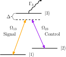
Figure 1: (Color online) Three-level atom in a $\Lambda$ configuration interacting with two fields in two-photon resonance via the common detuning $\Delta$, with spontaneous emission $\Gamma_{3}$ from the excited state.

II Mathematical Model

We consider the interaction of two fields with a $\Lambda$-system in two-photon resonance with each field addressing a different atomic transition as shown in Fig. 1. Each field interacts with the atomic system via the dipole moment operator which only links levels 1 to 3 and 2 to 3; $\hat{\vec{d}}=\vec{d}_{13}\left|1\right>\left<3\right|+\vec{d}_{23}\left|2\right>\left<3\right|+\vec{d}_{31}\left|3\right>\left<1\right|+\vec{d}_{32}\left|3\right>\left<2\right|$. We write the fields in carrier-envelope form:

$$\vec{E}(x,t)= \vec{\mathcal{E}}_{13}(x,t)e^{i(k_{13}x-\omega_{13}t)}$$

$$+\vec{\mathcal{E}}_{23}(x,t)e^{i(k_{23}x-\omega_{23}t)}+c.c$$ (2)

where $\omega_{13}$ and $\omega_{23}$ are the field frequencies, $k_{13}$ and $k_{23}$ the vacuum wave numbers and $\vec{\mathcal{E}}_{13}(x,t)$ and $\vec{\mathcal{E}}_{23}(x,t)$ the slowly-varying field envelopes. We assume that the envelopes change slowly over many cycles of the optical frequency, thus justifying the slow-varying envelope approximation (SVEA). Following Groves et al. (2013) we refer to the 1-3 field as the signal pulse and the 2-3 field as the control pulse. In the rotating-wave approximation (RWA) the bare frequencies $\omega_{13}$ and $\omega_{23}$ are eliminated in favor of $\Delta$, their common detuning, and the total Hamiltonian takes the form:

$$\hat{H}=-\frac{\hbar}{2}\left(\begin{array}[]{ccc}0&0&\Omega_{13}^{*}\\ 0&0&\Omega_{23}^{*}\\ \Omega_{13}&\Omega_{23}&-2\Delta\end{array}\right),$$ (3)

where we defined the Rabi frequencies, $\Omega_{13}(x,t)=2\vec{d}_{31}\cdot\vec{\mathcal{E}}_{13}(x,t)/\hbar$ and $\Omega_{23}(x,t)=2\vec{d}_{32}\cdot\vec{\mathcal{E}}_{23}(x,t)/\hbar$, and the detuning $\Delta=(E_{3}-E_{1})/\hbar-\omega_{13}=(E_{3}-E_{2})/\hbar-\omega_{23}$ ($E_{i}$ corresponds to the energy of level $\left|i\right>$). The dynamics of the system are dictated by the von Neumann equation for the density matrix of the atomic sample:

$$i\hbar\frac{\partial\hat{\rho}}{\partial t}=[\hat{H},\hat{\rho}],$$ (4)

and by Maxwell’s wave equation in the SVEA for the field evolution:

$$\left(\frac{\partial}{\partial x}+\frac{1}{c}\frac{\partial}{\partial t}\right)\Omega_{13} =i\mu_{13}\rho_{31}$$ (5a)

and

$$\left(\frac{\partial}{\partial x}+\frac{1}{c}\frac{\partial}{\partial t}\right)\Omega_{23} =i\mu_{23}\rho_{32}.$$ (5b)

Here, we defined the atom-field coupling parameters $\mu_{j3}=N\omega_{j3}|d_{j3}|^{2}/\hbar\epsilon_{0}c$ with $j=1,\,2$.

We consider the case of coherent short pulses for which it is justified to neglect homogeneous relaxation processes due to the fast interaction with the medium. This gives us a set of eight nonlinear partial differential equations that need to be solved simultaneously. As has been shown by Park and Shin Park and Shin (1998) and Clader and Eberly Clader and Eberly (2007), for the case of two-photon resonance and equal atom-field coupling parameters, $\mu_{13}=\mu_{23}=\mu$, the system of equations given by Eqs. (4) and (5) become integrable and thus can be solved by methods such as inverse scattering Lamb (1980), the Bäcklund transformation Miura (1976), and the Darboux transformation Gu et al. (2005); Cieśliński (2009). This can be easily shown by the introduction of the constant matrix

$$\hat{W}=i\left|3\right>\left<3\right|=\left(\begin{array}[]{ccc}0&0&0\\ 0&0&0\\ 0&0&i\end{array}\right),$$ (6)

so that Eqs. (4) and (5) in the traveling-wave coordinates $T=t-x/c$ and $Z=x$ can be expressed as:

$$i\hbar\frac{\partial\hat{\rho}}{\partial T}=[\hat{H},\hat{\rho}]$$ (7a)

and

$$\frac{\partial\hat{H}}{\partial Z}=-\frac{\hbar\mu}{2}[\hat{W},\hat{\rho}].$$ (7b)

By combining these two equations it is clear that the Lax equation,

$$\partial_{Z}\hat{U}-\partial_{T}\hat{V}+[\hat{U},\hat{V}]=0,$$ (8)

is satisfied where the Lax operators are defined as $\hat{U}=-(i/\hbar)\hat{H}-\lambda\hat{W}$ and $\hat{V}=(i\mu/2\lambda)\hat{\rho}$, and $\lambda$ is a constant known as the spectral parameter. This effectively shows that the Maxwell-Bloch equations (7) are integrable.

The solution obtained in Groves et al. (2013) is a second-order solution obtained from the nonlinear superposition of two first-order solutions, which in turn were obtained by means of the Darboux transformation from the trivial solution of a quiescent medium, $\hat{\rho}=\left|1\right>\left<1\right|$, and no fields, $\Omega_{13}=\Omega_{23}=0$. With an appropriate choice of parameters, this complicated solution can be reduced to a well-defined sequence of pulses interacting with the medium (see Fig. 2), transferring information back and forth.

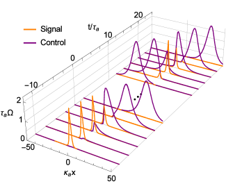
Figure 2: (Color online)Pulse evolution dictated by the second order analytical solution obtained by Groves et al. Groves et al. (2013). Appropriate parameters were chosen so that the intricate analytical solution could be simplified into a well-defined sequence of pulses, composed of two steps (separated by the ellipsis). In the first step, at $t/\tau_{a}=-10$, a $2\pi$-signal pulse comes in; and as it interacts with the medium, it gives way to a control pulse while storing its information at $\kappa_{a}x_{1}=0$. During the storage process, which takes place between $t/\tau_{a}=-7.5$ and $2.5$, the areas of the individual pulses are no longer equal to $2\pi$ but the total pulse area [see Eq. (9)] remains constant and equal to $2\pi$. At $t/\tau_{a}=2.5$ we can see that the initial $2\pi$ signal pulse is gone and has been taken over by a $2\pi$ control pulse propagating away at the speed of light. The second step starts at $t/\tau_{a}=12.5$ as a $2\pi$ control pulse comes in and collides with the information imprint left by the signal pulse. During the collision, which takes place between times $t/\tau_{a}=15$ and $22.5$, the initial signal pulse is retrieved and redeposited at $\kappa_{a}x_{2}=3$, effectively pushing the imprint farther into the medium. Here again, during the interaction the total pulse area is conserved and equal to $2\pi$. When the re-encoding has taken place, the control pulse recovers its original pulse area of $2\pi$ and propagates away at the speed of light. The corresponding imprint is depicted in Fig. 3.

As was done in Clader and Eberly (2007) we will define the total pulse area as

$$\theta_{\text{tot}}=\sqrt{|\theta_{13}|^{2}+|\theta_{23}|^{2}},$$ (9)

and we have that $\theta_{\text{tot}}=2\pi$ for the two first-order solutions. This concept can be extended to the second-order solution by applying it to the pulses in each step of the sequence, as long as they are sufficiently separated, as in Fig. 2 where the two steps are separated by an ellipsis. We will label the parameters pertaining to different steps of the sequence of pulses by the letters $a$ and $b$. For the first step, in the limit $t/\tau_{a}\ll-1$ we have a SIT-like signal pulse propagating, driving population from the ground state $\left|1\right>$ into the excited state $\left|3\right>$ and coherently driving it back, thus obtaining the characteristic $2\pi$ pulse shaped as an hyperbolic secant. As the control pulse is only zero in the limit of infinite negative time, some of the excited population is coherently driven into the ground state $\left|2\right>$, thus amplifying the seed of the control pulse and depleting the signal pulse. During this transfer the signal pulse encodes its information into the ground-state elements $\rho_{11}$, $\rho_{22}$, and $\rho_{12}$ of the density matrix. This encoding we refer to as an imprint. After the storage process is over we get a $2\pi$ control pulse propagating away at the speed of light as it is decoupled from the medium. Both signal and control pulses have a duration of $\tau_{a}$, and they are time-matched. Therefore the ratio between their Rabi frequencies is independent of time and given by:

$$\frac{\Omega_{13}^{a}(x,t)}{\Omega_{23}^{a}(x,t)}=e^{-\kappa_{a}(x-x_{1})},$$ (10)

where the absorption coefficient is given by $\kappa_{a}=\mu\tau_{a}/2$, since we are neglecting the effects of Doppler broadening, and $x_{1}$ is the location of the imprint. This relation shows us how we should map the analytical solution to appropriate initial conditions for the numerical computation. It is easy to see that, by integrating the previous equation with respect to $T$ and by considering that our medium starts at $x=0$, we can get $x_{1}$ in terms of the pulse areas:

$$\kappa_{a}x_{1}=\ln\left(\frac{\theta_{13}^{a}(x=0)}{\theta_{23}^{a}(x=0)}\right).$$ (11)

For the second step we start with a $2\pi$-control pulse of duration $\tau_{b}$ decoupled from the medium. When this control pulse collides with the imprint, the signal pulse is retrieved which, upon interaction with the medium, stores its information in a displaced location. When the re-encoding has taken place, the control pulse recovers its original pulse area of $2\pi$ and propagates away at the speed of light. The end result is the displacement of the imprint farther into the medium with a $\pi$-phase shift for $\rho_{12}$ if $\tau_{b}<\tau_{a}$. The displacement is controlled by the phase-lag parameter defined as:

$$\delta^{ab}=\kappa_{a}x_{2}-\kappa_{a}x_{1}=\ln\left|\frac{\tau_{a}+\tau_{b}}{\tau_{a}-\tau_{b}}\right|,$$ (12)

where $x_{2}$ is the new location of the imprint. Note that the addition of Doppler broadening would affect the definition of the absorption coefficient and thus change the group velocity of the pulses in the medium as was shown in Clader and Eberly (2007), but the storage procedure would carry through. The results of creation and displacement of the imprint are shown in Fig. 3. Continuous lines show the first imprinted density matrix elements, and the dashed lines show their displacements.

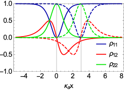
Figure 3: (Color online) Information encoding into a $\Lambda$-system: Imprint as it has been encoded in the ground state density matrix elements before (continuous lines) and after (dashed lines) the displacement. The imprint was generated by the pulse sequence depicted in Fig. 2, the snapshots were taken at times $t/\tau_{a}=5$ for the initial imprint and $t/\tau_{a}=25$ for the displaced one.

Having reviewed the main results of the analytical solution we now address the question of how these ideas can be used for storage and retrieval of optical pulses. The first step is to consider media of finite length and use Eq. (11) to determine the pulses’ input areas in order to store the signal pulse at the desired location. This location must be chosen so that most of the imprint fits inside the medium for optimal information storage. Signal pulse storage takes place as described by the dynamics of the first step in the sequence of pulses, where the control pulse overtakes the signal pulse. Now that we have the information stored inside the medium we want to be able to retrieve it. To do this we inject a second control pulse of area $2\pi$ and duration such that according to Eq. (12) the imprint is pushed outside the medium. When the control pulse collides with the imprint it retrieves the signal pulse that was stored in the medium, as described by the second step in the sequence. According to the previous results, the signal pulse travels until it reaches the location where the imprint is supposed to be re-encoded. However, this never takes place because the location lies outside the medium. Thus by frustrating the signal pulse re-storage by means of the end face of the medium we are able to retrieve it. Of course this retrieval can be done in any number of steps, displacing the imprint closer to the end face before retrieving it.

III Numerical Results

III.1 Initial considerations

The analytical solution is fairly restrictive because it assumes an infinite medium and $2\pi$ pulses with asymptotic hyperbolic secant shape with infinitely long tails. Additionally, we have neglected the effects of homogeneous relaxation phenomena and the atom-field coupling parameters were kept equal. Since we are considering the propagation of pulses in an ultra-cold atomic system, we can safely omit the effects of collisional and Doppler broadening, but spontaneous emission $\Gamma_{3}$ is still present and could have a noticeable effect. We modify the von Neumann equation (7a) to account for this:

$$\frac{\partial\rho_{11}}{\partial T}= \frac{i}{2}\Omega_{13}^{*}\rho_{31}-\frac{i}{2}\Omega_{13}\rho_{13}+\frac{\Gamma_{3}}{2}\rho_{33}$$ (13a)

$$\frac{\partial\rho_{22}}{\partial T}= \frac{i}{2}\Omega_{23}^{*}\rho_{32}-\frac{i}{2}\Omega_{23}\rho_{23}+\frac{\Gamma_{3}}{2}\rho_{33}$$ (13b)

$$\frac{\partial\rho_{33}}{\partial T}= -\frac{i}{2}\Omega_{13}^{*}\rho_{31}+\frac{i}{2}\Omega_{13}\rho_{13}-\frac{i}{2}\Omega_{23}^{*}\rho_{32}+\frac{i}{2}\Omega_{23}\rho_{23}$$

$$-\Gamma_{3}\rho_{33}$$ (13c)

$$\frac{\partial\rho_{12}}{\partial T}= \frac{i}{2}\Omega_{13}^{*}\rho_{32}-\frac{i}{2}\Omega_{23}\rho_{13}$$ (13d)

$$\frac{\partial\rho_{13}}{\partial T}= i\Delta\rho_{13}-\frac{i}{2}\Omega_{23}^{*}\rho_{12}+\frac{i}{2}\Omega_{13}^{*}(\rho_{33}-\rho_{11})-\frac{\Gamma_{3}}{2}\rho_{13}$$ (13e)

$$\frac{\partial\rho_{23}}{\partial T}= i\Delta\rho_{23}-\frac{i}{2}\Omega_{13}^{*}\rho_{21}+\frac{i}{2}\Omega_{23}^{*}(\rho_{33}-\rho_{22})-\frac{\Gamma_{3}}{2}\rho_{23}$$ (13f)

and for the field:

$$\frac{\partial\Omega_{13}}{\partial Z} =i\mu_{13}\rho_{31}$$ (14a)

$$\frac{\partial\Omega_{23}}{\partial Z} =i\mu_{23}\rho_{32}.$$ (14b)

The time and length scales are respectively defined in terms of the duration and absorption coefficient associated with the first signal pulse. We abandon the idealized conditions of infinitely long media and pulses by considering a medium ten absorption lengths long (unless otherwise noted) and setting the Rabi frequencies to zero when $|\tau_{a}\Omega|<10^{-5}$. For each simulation we will consider three cases: hyperbolic-secant-shaped pulses with no decay channels, Gaussian-shaped pulses with no decay channels, and hyperbolic-secant shaped pulses with decay channels. This allows the effects of shape and homogeneous broadening to be studied separately. The shape of the pulses we will use throughout are:

$$\Omega=\frac{\theta}{\pi\tau}\text{sech}\left(\frac{T}{\tau}\right)$$ (15a)

and

$$\Omega=\frac{\theta}{\sqrt{2\pi}\tau}e^{-\frac{T^{2}}{2\tau^{2}}}.$$ (15b)

For the simulations, we consider a sample of ⁸⁷Rb using the $D_{2}$ line and consider a pulse duration such that $\tau_{a}\Gamma_{3}=0.01$, so $\tau_{a}\approx 0.26\,\text{ns}$. For the atom-field coupling parameters we have that $\mu_{23}/\mu_{13}=0.99998$ Steck (2010a). From these estimates we clearly see that the approximations made in order to get the analytical solution were justified. Nonetheless we need to study their effects to determine whether these pulse dynamics are an experimentally realizable scenario. For simplicity the detuning is taken to be zero. Another thing worth noting is that we cannot choose an arbitrary pulse duration because we need to be able to resolve the hyperfine splitting of the ground state but not of the excited state in order to have a $\Lambda$-system. For the case of Rb we have the condition that $0.15\,\text{ns}<\tau_{a}<2\,\text{ns}$. We could have considered Cs atoms to attain smaller values for $\tau_{a}\Gamma_{3}$ by using shorter pulses, down to $0.1\,\text{ns}$ Steck (2010b). Or if we want to use longer pulses, we could use K but with the compromise of a larger value for $\tau_{a}\Gamma_{3}$($>0.03$) Tiecke (2011). Note that the important quantity is $\tau_{a}\Gamma_{3}$ and not just $\Gamma_{3}$, because what matters here is how long the spontaneous decay time is with respect to the interaction time between the pulses and the atomic system.

III.2 Location of initial imprint

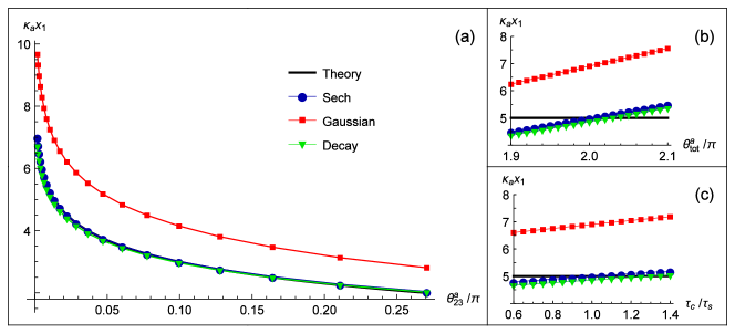
Figure 4: (Color online) Location of the initial imprint: (a) as a function of the control pulse area with a $2\pi$ signal pulse, (b) as a function of the total pulse area keeping the ratio of the pulses’ areas constant so that the predicted location is $\kappa_{a}x_{1}=5$, and (c) as a function of the duration of the control pulse with a $2\pi$ signal pulse and a predicted location of $\kappa_{a}x_{1}=5$. These plots compare the location of the initial imprint for four different cases. The black solid line is the formula given by the analytical solution, Eq. (11). The three plots with the markers represent the results of the numerical simulations for which we considered a medium ten absorption lengths long, finite pulses taking $\Omega=0$ when $|\tau_{a}\Omega|<10^{-5}$, and an initial $2\pi$ signal pulse. The plot with blue circle markers represents the case of a hyperbolic-secant pulse shape with $\tau_{a}\Gamma_{3}=0$, the one with green upside down triangle markers adds the effects of spontaneous emission to the previous one with $\tau_{a}\Gamma_{3}=0.01$, and finally the plot with red square markers considers a Gaussian-shaped pulse with $\tau_{a}\Gamma_{3}=0$.

First, we consider how the shape and finiteness of the pulses, as well as the effects of homogeneous relaxation, affect the location of the first imprint. The results of the numerical simulations are summarized in Fig. 4. For the dependence on the control pulse area, Fig. 4(a), we notice that the hyperbolic secant-shaped pulse completely overlaps the curve given by the theory. We see that the effect of spontaneous emission is to lower the curve very slightly while maintaining the same shape. The Gaussian-shaped pulse clearly deviates from the expected behavior, but keeps a predictable trend and in the grand scheme has the same dependence, i.e., the location of the imprint increases when the control pulse area decreases. The effects of spontaneous emission on the Gaussian-shaped pulse curve are analogous to those of the hyperbolic secant-shaped pulse, namely, to lower the curve while keeping the same type of dependence (the data for this case are not presented for the sake of clarity in the figures).

The analytical solution sets the total pulse area of each step of the process equal to $2\pi$, but we are free to change that in the simulations. From an experimental point of view, it is important to know this dependence, since it might be difficult to control the area of the pulses with much precision. Setting the ratio of the signal to control pulse area such that Eq. (11) predicts an imprint location of $\kappa_{a}x_{1}=5$, we vary the total pulse area [see Fig. 4(b)]. We find that for all three cases there appears to be a linear dependence with similar positive slope, $\Delta(\kappa_{a}x_{1})/\Delta\theta_{\text{tot}}^{a}\approx 5/\pi$ for the hyperbolic secant shaped- and $\Delta(\kappa_{a}x_{1})/\Delta\theta_{\text{tot}}^{a}\approx 6.5/\pi$ for the Gaussian-shaped pulses. Here we only consider small variations inherent to any realistic experimental scenario and so this behavior cannot be extrapolated to arbitrarily large and small pulse areas. In particular, if we consider areas smaller than $\pi$ then the pulses are not strong enough to promote the necessary population transfer for the initial SIT propagation and then the transfer from signal to control pulses. For pulse areas larger than $3\pi$ we would get pulse breakup and thus a different kind of interaction.

Another restriction from the solution is that signal and control pulses are time matched (this might not be ideal for an experiment because one would have to change the duration of the control pulses between consecutive steps). Relaxing this condition we find a behavior similar to the previous case [see Fig. 4(c)]: the imprint location increases with the duration of the control pulse. Once again all three cases seem to have similar positive slopes, $\Delta(\kappa_{a}x_{1})/\Delta(\tau_{c}/\tau_{s})\approx 0.5$ for the hyperbolic secants and $\Delta(\kappa_{a}x_{1})/\Delta(\tau_{c}/\tau_{s})\approx 0.73$ for the Gaussian. It is also worth mentioning that the shape of the imprint is the same as the one predicted theoretically (Fig. 3) for the two cases where the pulses are hyperbolic secants, but for the Gaussian-shaped pulse it is approximately $1.4$ times wider. This is a consequence of the reshaping of the Gaussian pulse to a corresponding hyperbolic-secant-shaped pulse with slightly different time duration.

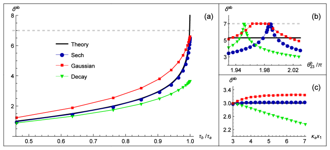
Figure 5: (Color online) Displacement of the imprint as a function of: (a) the duration of the second control pulse, (b) the control pulse area, and (c) the location of the initial imprint. We consider the same three cases as those described in Fig. 4, represented by the same markers. For (a) and (b) we considered an initial $2\pi$ signal pulse with the necessary pulse area of the corresponding control pulse so that the location of the first imprint is at $\kappa_{a}x_{1}=3$. Then for (a) we kept the area of the second control pulse equal to $2\pi$. The dashed light gray line marks the end of the medium and the black solid line is the result predicted by Eq. (12). For (c) we considered a longer medium, 15 absorption lengths long, and we chose the control pulse duration so that we had a displacement of $\delta^{ab}=3$ when the initial imprint was at $\kappa_{a}x_{1}=3$.

III.3 Displacement of the imprint

Now that we know we can imprint the information of the signal pulse into the atomic system given non-idealized conditions, we have to study the next step of the pulse sequence: the displacement of the imprint. To do this, we select the initial pulse area of the control pulse for each case using the results from the previous section, so that the initial imprint is made at $\kappa_{a}x_{1}=3$ combined with a $2\pi$ signal pulse. Then we vary the control pulse duration and find the new position of the imprint. The results are summarized in Fig. 5(a).

As predicted by the theory, the closer $\tau_{b}$ is to $\tau_{a}$, the more the imprint is displaced. Additionally, the new imprint is identical to the initial one except for a $\pi$ phase shift when the control pulse duration is smaller than the signal pulse. We also notice that the different parameters affect the displacement in a similar way regarding the location of the initial imprint. The hyperbolic-secant-shaped pulse closely follows the behavior dictated by Eq. (12), while the addition of decay causes a decrease in the displacement. However, the Gaussian-shaped pulse causes a displacement that is typically larger than that given by the analytical solution (here again the effects of spontaneous emission for the Gaussian-shaped pulse are analogous to those of the hyperbolic-secant-shaped pulse). The biggest difference from the theoretical prediction is that there is an upper limit in how much the imprint can be moved (this is true for all three cases). This will define how close the imprint must be to the end face so that the signal pulse can be retrieved. Another feature is that if we consider the case $\tau_{b}>\tau_{a}$ we get similar results but the imprint does not present the $\pi$ phase shift. This might be desirable if we want the retrieved signal pulse to have the same phase as the original (as we will see in the next section), but one must be careful because homogeneous relaxation will affect the displacement even more if the pulses interact with the medium for a longer time.

We also explore the dependence of the displacement with respect to the control pulse area $\theta_{23}^{b}$ as noted before, a parameter not accessible from the analytical solution. As shown in Fig. 5(b), the results are quite surprising. We find that the displacement increases as we decrease the pulse area, until it reaches a maximum (these are hidden by the plateaus which represent that the imprint has been pushed outside the medium) and then starts decreasing again. For all three cases, the “optimal” pulse area is actually less than the $2\pi$ predicted by the theory, and not only do we have maxima for these smaller areas but also the displacement can be much greater than the one predicted in Eq. (12).

There is also some dependence on the first imprint location, and there are two possible tendencies as shown in Fig. 5(c). The first is an increase in the displacement as we increase $x_{1}$ until it reaches a steady value. This behavior is obtained when there are no decay channels and is due to the finiteness of the medium which cuts off part of the information deposited by the signal pulse, so the closer we get to the center of the medium the more room there is for the imprint to be made. As for the Gaussian-shaped pulse, it is affected the most because the imprint is wider. When we consider spontaneous emission, another process takes over: The further into the medium the first imprint is made, the less it will be displaced by the second control pulse. This can be understood by the fact that the longer it takes to deposit the information of the signal pulse, the longer the decay is effective, provoking some information loss and this ultimately leads to less displacement.

III.4 Retrieval of the signal pulse

One of the most important effects of the boundaries in the medium is to cut off the pulse transfer process of the analytical solution, thus providing a way to retrieve the initial signal pulse. To quantify the accuracy of the retrieval process we define the retrieval efficiency as

$$\eta=\frac{I_{13}^{\text{out}}}{I_{13}^{\text{in}}}=\frac{\int|\Omega_{13}^{\text{out}}|^{2}dt}{\int|\Omega_{13}^{\text{in}}|^{2}dt}.$$ (16)

Clearly this quantity only gives information about the output signal pulse intensity but does not take into account any possible reshaping of the pulse. To account for this we calculate the correlation coefficient $r$ between the input and output signal pulses. This is particularly important for the Gaussian-shaped pulses which are reshaped into hyperbolic secants as they propagate through the medium. This has already been noted in the case of atomic vapors at room temperature Clader and Eberly (2007, 2008). From the previous sections it should be clear that the retrieval process can take place in any number of steps, but for the sake of clarity we will treat only two cases: two- and three-step retrieval. Additionally, we will only consider control pulses of areas equal to $2\pi$ and of duration times equal to or smaller than that of the initial signal pulse for the displacement and retrieval steps.

Table 1: Retrieval efficiency and correlation coefficient for one- and two-step processes.

Case	1 step		2 steps
	$\eta$	$r$	$\eta$	$r$
Sech	98%	1.0000	98%	1.0000
Decay	65%	0.9998	66%	0.9998
Gaussian	94%	0.9940	94%	0.9941

Let us first consider the one-step process. Here we want to make the imprint somewhere in the medium such that it can be retrieved without having to move it closer to the boundary (this limit is set by the case where we consider homogeneous relaxation). For this we consider the necessary pulse areas for each case so that the initial imprint is made at $\kappa_{a}x_{1}=8$, and for the second step we consider a control pulse with the same duration as the signal pulse, giving us the maximum displacement. For the two-step process we will make the initial imprint at $\kappa_{a}x_{1}=5$, then tailor the time duration of the following control pulse so that we displace the imprint by $\delta^{ab}=3$ and finally push the imprint outside the medium by means of another control pulse of duration equal to the original signal pulse. The results are summarized in Table 1. We notice that, when no decay is present, the efficiency is high (larger than 90%) but as soon as homogeneous relaxation is added it drops to 65% for one-step and 66% for two-step processes. As for the correlation coefficient, it is fairly close to unity in all cases, indicating that the shape of the pulse is mostly preserved throughout the storage and retrieval procedure. The Gaussian-shaped pulses are the ones that have the lowest $r$ values as could have been expected because of the reshaping during propagation. In any case, we are able to retrieve a good portion of the initial signal pulse and see that this does not depend on the number of steps involved. In the one-step case, the retrieved signal pulse has a $\pi$ phase shift with respect to the original. The correct phase can be obtained by inverting the initial storing control pulse or by increasing the duration of the second control pulse as discussed in Sec. III.3. In the two-step process, the signal pulse comes out with the same phase due to the $\pi$-phase shift in the displacement step.

IV Conclusions

In this report we have shown that previously predicted memory manipulation by means of idealized atomic pulse dynamics is plausible even in non-idealized conditions. The shape of the pulse and the effects of spontaneous emission have an impact on the quantitative results but the storage and retrieval of the signal pulse are achieved in all cases. We have quantified the deviations in each case and even shown some features that could add more control to the process and lift some restrictions. The length of the medium has no effect on the memory manipulation, but should be chosen so that most of the information can be deposited into the medium. This may no longer be true if we consider the reflection of the pulses at the end face.

Another aspect that we noticed throughout this work, and that has been noted elsewhere, is the stability against the total pulse area. When considering pulses of different area than $2\pi$, be it bigger or smaller, the pulses are reshaped as they propagate in an effort to obtain a $2\pi$ total area. This is completely analogous to the predictions of the area theorem McCall and Hahn (1967, 1969) for a homogeneously broadened two-level atom. Additionally, we can ask which is the appropriate extension of the total pulse area for higher order solutions, particularly when the two first- order solutions overlap.

We can also think of extending this analysis to more complicated pulse sequences. This would be the same as simulating higher-order solutions of the Maxwell-Bloch equations obtained by further applications of the nonlinear superposition rule. This could possibly pave the way for making multiple imprints belonging to different signal pulses and then manipulating them by means of control pulses.