Description of light nuclei in pionless effective field theory using the stochastic variational method

Abstract

We construct a coordinate-space potential based on pionless effective field theory (EFT) with a Gaussian regulator. Charge-symmetry breaking is included through the Coulomb potential and through two- and three-body contact interactions. Starting with the effective field theory potential, we apply the stochastic variational method to determine the ground states of nuclei with mass number $A\leq 4$. At next-to-next-to-leading order, two out of three independent three-body parameters can be fitted to the three-body binding energies. To fix the remaining one, we look for a simultaneous description of the binding energy of ⁴He and the charge radii of ³He and ⁴He. We show that at the order considered we can find an acceptable solution, within the uncertainty of the expansion. We find that the EFT expansion shows good agreement with empirical data within the estimated uncertainty, even for a system as dense as ⁴He.

I Introduction

The idea of an effective field theory (EFT) is now firmly entrenched in physics: it provides a systematic way to describe a quantum system using the relevant degrees of freedom at some low-energy scale, combined with a systematic expansion in powers of that scale divided by a reference scale. The use of such theories in nuclear physics takes its cue from the work of Weinberg Weinberg:1990rz ; Weinberg:1991um . The original formulation is in terms of nucleons and pions and is based on expansions in ratios of small momenta or the pion mass to a typical QCD scale, such as the mass of the $\rho$ meson .

For momentum scales that are even smaller than the pion mass $m_{\pi}$, as they are in the ground states of the lightest nuclei, we can reduce the degrees of freedom still further and work with a pionless EFT Kaplan:1998xu ; Chen:1999tn ; Bedaque:2002mn . This is constructed in terms of contact interactions involving two or more nucleons, ordered in powers of $Q=p/m_{\pi}$, where $p$ is a typical nucleon momentum. At each order in the expansion new counter terms appear, and these need to be fixed from experimental data. A similar approach should also be applied to other observables to derive effective operators that are consistent with the effective interactions.

A key feature of the nucleon-nucleon interaction is the strong attraction in $S$-waves. This is signalled by the scattering lengths which are unnaturally large compared to the scale of the underlying physics, $1/m_{\pi}$. This means that the inverses of these scattering lengths provide additional low-energy scales and the power counting must be modified to take account of these scales. The leading $S$-wave contact terms are then of order $Q^{-1}$, which means that they can not be treated perturbatively, and have to be resummed to all orders. The resulting expansion of the scattering amplitude is just the long-established effective range expansion Bethe .

The first applications of this EFT to few-nucleon systems were to the triton Bedaque:1998kg , and used the Skorniakov–Ter-Martirosian equation Skorniakov . A disadvantage of this approach is that it does not provide easy access to the full wave function of the system. Calculations of observables in the framework can become somewhat complex, as can be seen, for example, in the recent work of Vanasse Vanasse:2015fph .

One alternative is to use an approach based on a Hamiltonian formulation of the EFT. The pionless EFT has previously been treated by Platter et al. Platter:2004zs using the Yakubovsky equations, and by Kirscher et al. Kirscher:2009aj using a variational approach based on the resonating-group method Tang:1978zz ; Hoffmann:1987 . Such variational methods have a long tradition in studies of few-nucleon systems with finite-range forces. (For a review, see Ref. Kievsky:2008es .)

In our calculations, we employ one of these approaches, the stochastic variational method (SVM) Suzuki:1998bn . This is a method for finding bound-state solutions to the Schrödinger equation, which has proved powerful in a variety of contexts. As in the case of the resonating-group method, this starts from a Hamiltonian formulation of the EFT, rather than a Lagrangian one. It is also easiest to apply when the short-range interactions are expressed in the form of a local potential in coordinate space. Kirscher et al. achieved this by employing a Gaussian regulator Kirscher:2009aj . We follow the same approach here since such a regulator is especially well suited to the SVM.

We work at next-to-next-to-leading order (NNLO) in the pionless EFT, with a Hamiltonian that contains two- and three-nucleon interactions and the Coulomb potential. Using the SVM to solve the Schrödinger equation provides bound-state wave functions as well as energies for nuclei with $A=3$ and $4$. With these wave functions, we calculate charge radii to the same order in the expansion. The basic calculations of the ground-state energies are similar to those of Kirscher et al. Kirscher:2009aj ; the main difference between our approaches is that we explore a consistent description of energies and other observables at the same level of truncation. We also look more closely at ambiguities in the parameter fits.

Solving an EFT by use of the Schrödinger equation implicitly iterates all terms in the interaction to all orders. This is rather different from the strict perturbative expansion that has been implemented within the Lagrangian approach, e.g., Konig:2015aka . Iterating the potential in this way generates higher-order contributions to observables that are in principle beyond the accuracy of our treatment. However, provided that the expansion of the EFT is converging, these contributions should be within the uncertainty of our truncation of the theory. The iteration also means that the parameters are only implicitly renormalised by fitting them to observables. One has to be careful: such a procedure can break down if the regulator scale is taken above the scale of the underlying physics Epelbaum:2009sd ; Birse:2009my .

In our approach we first fit two-body potentials to low-energy nucleon-nucleon phase shifts. The short-range potentials are regulated by a Gaussian function whose width plays the role of a cut-off scale. Varying this width generates a set of potentials that all describe the same two-body data. We use the dependence on the cut-off scale to determine where our approach breaks down and to estimate the uncertainties on our results. We also include charge-symmetry breaking (CSB), in particular from the Coulomb potential, but also from the contact interaction that is needed to renormalise the $pp$ scattering length Kong:1998sx ; Kong:1999sf .

We then add a three-body potential and examine the three-nucleon systems ³H and ³He. When Coulomb effects are included, a CSB three-body interaction is also required Vanasse:2014kxa , leading to a potential with three free parameters. Only two of these can be determined from the ground-state energies. Varying the remaining parameter allows us to explore parametric relations between the energies and charge radii of nuclei with $A=3$ and $4$.

The article is structured as follows. First we set out, in Sec. II, the details of the effective theory that we use, and give expressions for the relevant two- and three-body potentials. We then outline, in Sec. III, the important features of the stochastic variational method (SVM), which we use to solve the Schrödinger equation for the bound states of three- and four-nucleon systems. The determination of the two-body parameters from scattering phase shifts is discussed in Sec. IV. Then, in Sec. V, we apply the SVM to the ground states of ³H, ³He and ⁴He, and we present our results for their properties. We finally discuss some implications of our results in Sec. VI. Details of the Kohn variational principle used in the two-nucleon sector and an analysis of convergence are contained in the appendices.

II Pionless EFT

We work with the pionless EFT at next-to-next-to-leading order (NNLO), using the power counting for systems with anomalously large $S$-wave scattering lengths Kaplan:1998xu ; Bedaque:2002mn . To NNLO, the effective Lagrangian consists of two- and three-body contact interactions containing up to two derivatives. The resulting nucleon-nucleon interaction can be expressed as a momentum-space potential with the following form (see, for example, Refs. Ordonez:1995rz ; Kirscher:2009aj ):

$$\begin{split}V_{NN}=&\,\frac{1}{2}\sum_{i\neq j}\Bigl{[}C_{1}+C_{2}\,\boldsymbol{\sigma}_{i}\cdot\boldsymbol{\sigma}_{j}+D_{1}q^{2}+D_{2}k^{2}+\boldsymbol{\sigma}_{i}\cdot\boldsymbol{\sigma}_{j}\left(D_{3}q^{2}+D_{4}k^{2}\right)\\ &+\frac{1}{2}D_{5}\left(\boldsymbol{\sigma}_{i}+\boldsymbol{\sigma}_{j}\right)\cdot\boldsymbol{q}\times\boldsymbol{k}+D_{6}(\boldsymbol{q}\cdot\boldsymbol{\sigma}_{i})(\boldsymbol{q}\cdot\boldsymbol{\sigma}_{j})+D_{7}(\boldsymbol{k}\cdot\boldsymbol{\sigma}_{i})(\boldsymbol{k}\cdot\boldsymbol{\sigma}_{j})\Bigr{]}\,,\end{split}$$ (1)

where for each pair $ij$, $\boldsymbol{q}=\boldsymbol{p}_{i}-\boldsymbol{p}_{i}^{\prime}$ and $\boldsymbol{k}=(\boldsymbol{p}_{i}+\boldsymbol{p}_{i}^{\prime})/2$ are defined in terms of the initial and final centre-of-mass momenta of one of the nucleons, $\boldsymbol{p}_{i}$ and $\boldsymbol{p}_{i}^{\prime}$. Note that $\boldsymbol{q}$ is just the difference between the relative momenta of the two nucleons before and after the interaction, whereas in the two-body centre-of-mass frame $\boldsymbol{k}$ is the average of these momenta.

For systems with very strong $S$-wave scattering at low energies, the large scattering lengths should be counted as of order $Q^{-1}$ Kaplan:1998xu ; Bedaque:2002mn . That is the case for nucleon-nucleon scattering, and thus the leading-order (LO) $S$-wave contact interactions ($C_{1}$ and $C_{2}$) are of order $Q^{-1}$ and hence need to be treated nonperturbatively. The higher-order interactions are also enhanced relative to a naïve power counting, and their orders can be obtained from an expansion around a non-trivial fixed point of the renormalisation group Birse:1998dk . In particular, the subleading $S$-wave contact interactions are promoted by two powers of $Q$ relative to naïve dimensional analysis, and terms that couple $S$-waves to other channels, such as the $S$–$D$ mixing, are promoted by one power.

At next-to-leading order (NLO), we find the momentum-dependent $S$-wave interactions, $D_{1}$ to $D_{4}$, which enter at $\mathcal{O}(Q^{0})$. At NNLO or $\mathcal{O}(Q^{1})$, the tensor interactions $D_{6}$ and $D_{7}$ contribute to $S$–$D$ mixing. The $D_{5}$ term describes the spin-orbit interaction, and so does not contribute in $S$-waves interactions, hence we ignore it as it enters only at $\mathcal{O}(Q^{2})$. We also omit the $D_{7}$ term, which generates a non-local tensor interaction, since its effects cannot be distinguished from those of the local $D_{6}$ term to the order we work here; disentangling them would require data on $P$ waves, whose amplitudes start at $\mathcal{O}(Q^{2})$.

As a further simplification, we also make use of the fact that the total spin and isospin of the nucleon-nucleon partial waves are correlated and so there is some freedom in the choice of the spin and isospin operators, as pointed out in, for example, Refs. Weinberg:1990rz ; Ordonez:1995rz . A recent discussion can be found in Ref. Gezerlis:2014zia , which makes a slightly different choice from ours. Since the tensor interaction couples $S$ and $D$ waves with spin-1 and isospin-0, we choose an isospin structure that projects the $D_{6}$ term onto isospin-0. Finally, for the central interactions, we keep only terms with the isospin-dependent form $\boldsymbol{\tau}_{i}\cdot\boldsymbol{\tau}_{j}$. These choices simplify the fitting of the potential to empirical data.

In order to to make use of this potential in the SVM, which works in coordinate space, we take its Fourier transform. At this step we introduce a local Gaussian regulator,

$$G(r,\sigma)=\exp\left(-\frac{1}{2}\frac{r^{2}}{\sigma^{2}}\right),$$ (2)

similar to that used by Kirscher et al. Kirscher:2009aj . The resulting coordinate-space potential has the form

$$\begin{split}V_{NN}=&\sum_{i<j}\Bigl{\{}G(r_{ij},\sigma)\left(A_{1}+A_{2}\boldsymbol{\tau_{i}}\cdot\boldsymbol{\tau_{j}}\right)+r_{ij}^{2}G(r_{ij},\sigma)\left(A_{3}+A_{4}\boldsymbol{\tau_{i}}\cdot\boldsymbol{\tau_{j}}\right)\\ &\qquad+\left\{\nabla_{ij}^{2},G(r_{ij},\sigma)\right\}\left(A_{5}+A_{6}\boldsymbol{\tau_{i}}\cdot\boldsymbol{\tau_{j}}\right)\\ &\qquad+G(r_{ij},\sigma)A_{7}\left(1-\boldsymbol{\tau_{i}}\cdot\boldsymbol{\tau_{j}}\right)\left[3(\hat{\boldsymbol{r}}_{ij}\cdot\boldsymbol{\sigma}_{i})(\hat{\boldsymbol{r}}_{ij}\cdot\boldsymbol{\sigma}_{j})-(\boldsymbol{\sigma}_{i}\cdot\boldsymbol{\sigma}_{j})\right]\Bigr{\}}\,,\end{split}$$ (3)

where $\boldsymbol{r}_{ij}=\boldsymbol{r}_{i}-\boldsymbol{r}_{j}$, $\hat{\boldsymbol{r}}_{ij}$ is the corresponding unit vector, and $\{\nabla^{2},G(r,\sigma)\}$ stands for the commutator of the two operators acting on the wave function. The parameters $A_{i}$ are linear combinations of the $C_{i}$ and $D_{i}$, showing the mixing between orders in a potential model. Note that the tensor interaction has been explicitly projected out of the isospin-1 channel. The non-local terms give rise to derivative operators in Eq. (3), see, for example, Ref. Nagels:1977ze .

We also include the long-range Coulomb potential that acts between protons,

$$V_{pp}^{\mathrm{C}}=\frac{\alpha_{\mathrm{em}}}{r_{ij}}\,,$$ (4)

where $\alpha_{\mathrm{em}}$ is the fine structure constant. Two choices of power counting are possible for this potential. For the first choice one identifies the scale related to its strength, $\alpha_{\mathrm{em}}M$, with $M$ being the nucleon mass, as a low-energy scale, of order $Q$. This makes the Coulomb potential $\mathcal{O}(Q^{-1})$ and so it should be resummed to all orders, as required in order to properly describe, for instance, very-low-energy proton-proton scattering Kong:1998sx ; Kong:1999sf . In this scheme, there is a $pp$ CSB contact interaction proportional to $\alpha_{\mathrm{em}}$ which also appears at order $\mathcal{O}(Q^{-1})$ and is needed to renormalise the $pp$ scattering length. This approach was used in Ref. Ando:2010wq and more recently by Vanasse Vanasse:2014kxa in studies of three-nucleon systems. Applications to these systems require an additional CSB three-body force of order $\mathcal{O}(Q^{0})$.

However the typical momenta in the three-body bound states are significantly larger than $\alpha_{\mathrm{em}}M$, suggesting a second choice where the Coulomb interaction can be treated perturbatively, as proposed by Rupak and Kong Rupak:2001ci and confirmed in more detailed work by König et al. Konig:2015aka . This can be implemented in the EFT framework by taking $\alpha_{\mathrm{em}}M$ to be $\mathcal{O}(Q^{2})$, making the Coulomb potential itself of order $Q^{0}$. In this counting scheme the CSB two- and three-body contact interactions appear at one order higher in $Q$ than in the Kong and Ravndal version: $\mathcal{O}(Q^{0})$ and $\mathcal{O}(Q^{1})$ respectively.

In either case, we need to take account of the CSB contact interactions. In the two-nucleon sector, we add the following interactions to the $pp$ channel:

$$V_{pp}^{\mathrm{CSB}}=G(r_{ij},\sigma)A_{1}^{\mathrm{CSB}}+r_{ij}^{2}G(r_{ij},\sigma)A_{3}^{\mathrm{CSB}}+\left\{\nabla_{ij}^{2},G(r_{ij},\sigma)\right\}A_{5}^{\mathrm{CSB}}\,.$$ (5)

These forces modify the strong interaction between two protons and renormalise the effects of the Coulomb potential. Since we implicitly treat that potential to all orders, we include a CSB contribution to the $pp$ effective range and we find that it is needed to give a good description of the low-energy $pp$ phase shift. However, in the counting scheme where the Coulomb potential is treated perturbatively, that term would be of order $Q^{2}$ and so, strictly speaking, it would be beyond the accuracy of our current treatment.

We solve the Schrödinger equation with the regulated potential and fit the coefficients $A_{i}$ and $A_{i}^{\mathrm{CSB}}$ to data from low-energy nucleon-nucleon scattering. Since the potential is treated to all orders in this procedure, we rely on an implicit renormalisation of the parameters, as outlined by Gasser and Leutwyler Gasser:1982ap and discussed further in Ref. Epelbaum:2009sd . Resumming the potential generates terms in the amplitude that are beyond the order of our truncation. It has long been known that these can cause problems if the regulator has too short a range Scaldeferri:1996nx ; Phillips:1996ae . However, provided the momentum scale of the regulator is not taken above the breakdown scale of the EFT, these higher order terms are within the error of the truncation. On the other hand regulating the theory at much lower scales or longer distances can generate large artefacts of the cut-off. Reconciling these conflicting demands suggests that the regulator scale should be chosen just below the breakdown scale of the EFT Epelbaum:2009sd ; Birse:2009my .

In the case of the pionless EFT, we expect the appropriate scale to be of the order of $1/m_{\pi}$. The precise value will depend on the the chosen form of the regulator. For instance, a lower bound of $R=1.3$ fm was found for a sharp radial cut-off in Ref. Scaldeferri:1996nx . Here we explore several choices for the parameter $\sigma$ in the range 0.6 to 1.2 fm. We examine how the fitted values of the coefficients vary with the width of the Gaussian regulator, $\sigma$, and exclude the region where these coefficients start to become “unnaturally” large. This is contrast to the recent work by Kirscher and Gazit Kirscher:2015zoa who use a similar potential to ours but with cut-offs corresponding to $\sigma$ in the range 0.08 to 0.25 fm. Treating the NLO potential to all orders with such cut-offs requires a high degree of fine-tuning, and runs the risk of generating unphysical features such as producing an additional, deeply bound, three-nucleon state.

We now turn our attention to three-nucleon systems. In these, three-body forces have been shown to be needed at leading order in the pionless EFT in order to renormalise observables such as the triton binding energy Bedaque:1998kg . This, in turn, can be related to the Efimov effect — a geometric sequence of bound states seen in the symmetric $S$-wave channels of three particles interacting via contact interactions Efimov:1970zz . In EFT treatments of such systems, the leading three-nucleon interaction exhibits limit-cycle behaviour Bedaque:1998kg and so has an anomalous power counting of $\mathcal{O}(Q^{-1})$ Barford:2004fz .

At LO there is only one independent spin-isospin structure in the three-body contact interaction since all possible combinations of spin and isospin operators give equivalent results when they act on antisymmetrised wave functions Bedaque:2002yg ; Epelbaum:2002vt . Taking advantage of this equivalence, we work with the isospin- and spin-independent expression,

$$V_{3N}^{\mathrm{LO}}=\sum_{i<j<k}E_{1}\,,$$ (6)

for the LO three-body potential. We fix the strength of this interaction, $E_{1}$, by fitting it to the triton binding energy.

At NLO, a $\mathcal{O}(Q^{0})$ three-nucleon force is needed only in order to properly renormalise the effects of the two-body effective range; since this does not introduce either new spin-isospin structures or dependence on the nucleon momenta, it cannot be separated from the LO potential.

Finally, at NNLO we need to include three-nucleon forces that are quadratic in the nucleon momenta. The corresponding potential contains ten independent structures Girlanda:2011fh :

$$\begin{split}V_{3N}^{\mathrm{NNLO}}=&\sum_{i\neq j\neq k}\Bigl{[}\ q_{i}^{2}\left(F_{1}+F_{2}\boldsymbol{\tau}_{i}\cdot\boldsymbol{\tau}_{j}+F_{3}\boldsymbol{\sigma}_{i}\cdot\boldsymbol{\sigma}_{j}+F_{4}\boldsymbol{\sigma}_{i}\cdot\boldsymbol{\sigma}_{j}\boldsymbol{\tau}_{i}\cdot\boldsymbol{\tau}_{j}\right)\\ &\qquad+\left[3(\boldsymbol{q}_{i}\cdot\boldsymbol{\sigma}_{i})(\boldsymbol{q}_{i}\cdot\boldsymbol{\sigma}_{j})-q_{i}^{2}\right](F_{5}+F_{6}\boldsymbol{\tau}_{i}\cdot\boldsymbol{\tau}_{j})\\ &\qquad+\frac{1}{2}(\boldsymbol{\sigma}_{i}+\boldsymbol{\sigma}_{j})\cdot\boldsymbol{q}_{i}\times(\boldsymbol{k}_{i}-\boldsymbol{k}_{j})(F_{7}+F_{8}\boldsymbol{\tau}_{j}\cdot\boldsymbol{\tau}_{k})\\ &\qquad+(\boldsymbol{k}_{i}\cdot\boldsymbol{\sigma}_{i})(\boldsymbol{k}_{j}\cdot\boldsymbol{\sigma}_{j})(F_{9}+F_{10}\boldsymbol{\tau}_{i}\cdot\boldsymbol{\tau}_{j})\Bigr{]}\,,\end{split}$$ (7)

where $\boldsymbol{q}_{i}=\boldsymbol{p}_{i}-\boldsymbol{p}_{i}^{\prime}$ and $\boldsymbol{k}_{i}=(\boldsymbol{p}_{i}+\boldsymbol{p}_{i}^{\prime})/2$ are defined in terms of the centre-of-mass momenta of one nucleon, as in the two-body case. However, some of these structures couple only to higher partial waves which do not receive the enhancement present in the spatially symmetric $S$-wave channel Griesshammer:2005ga . They therefore contribute only at higher orders and we neglect them. These are the terms proportional to $F_{5,6}$ and $F_{9,10}$, the three-body tensor interaction and its recoil corrections, and the ones containing $F_{7,8}$, the three-body spin-orbit force.

This leaves four momentum-dependent structures proportional to $F_{1\dots 4}$. These are equivalent if the nuclear wave function is symmetric under exchange of the momenta of any two nucleons. Since the ground-state wave functions of the nuclei we study — ³H, ³He, ⁴He — are dominated by the spatially symmetric $S$-wave channel, we can choose one of the terms $F_{1\dots 4}$ to represent the effect of the $\mathcal{O}(Q^{1})$ three-nucleon potential. Guided by this, we choose the following symmetric form,

$$V_{3N}^{\mathrm{NNLO}}=\sum_{i<j<k}F_{1}(q_{i}^{2}+q_{j}^{2}+q_{k}^{2})\,.$$ (8)

As in the two-body case, we express this potential in coordinate space using a Gaussian regulator, with the additional requirement that it should depend on relative momenta only and be symmetric with respect to interchange of any two particles. The use of a local form for the regulator can break the equivalence of the different possible spin-isospin structures, as observed by Lynn et al. Lynn:2015jua . More specifically, as those authors point out, this dependence on the spin-isospin structure shows up in the $P$-wave states, where three-body forces are of higher-order than considered here.

For simplicity, we choose the range parameter of our regulator to be the same as in the two-body potential. This leads to the following coordinate-space form for the three-body potential, including both LO and NNLO terms:

$$V_{3N}=\sum_{i<j<k}\left[B_{1}+B_{2}\frac{1}{\sigma^{2}}\left(r_{ij}^{2}+r_{ik}^{2}+r_{jk}^{2}\right)\right]\exp\left(-\frac{1}{2\sigma^{2}}\left(r_{ij}^{2}+r_{ik}^{2}+r_{jk}^{2}\right)\right)\,,$$ (9)

This can also be expressed in Jacobi coordinates,

$$\boldsymbol{\xi}_{1}=\frac{1}{\sqrt{2}}(\boldsymbol{r}_{i}-\boldsymbol{r}_{j}),\quad\boldsymbol{\xi}_{2}=\sqrt{\frac{2}{3}}\left(\frac{1}{2}(\boldsymbol{r}_{i}+\boldsymbol{r}_{j})-\boldsymbol{r}_{k}\right)\,;$$ (10)

with the help of the relation

$$\xi_{1}^{2}+\xi_{2}^{2}=\left(r_{ij}^{2}+r_{ik}^{2}+r_{jk}^{2}\right)/3\,.$$ (11)

Finally, the inclusion of the Coulomb potential in the proton-proton sector leads to CSB in the three-nucleon interaction. In particular, renormalising the three-body interaction in the presence of a Coulomb force leads to a contact term proportional to $\alpha_{\mathrm{em}}$. As discussed above, iterating the Coulomb potential corresponds to treating $\alpha_{\mathrm{em}}M$ as being of order $Q$, and so this interaction appears at NLO or $\mathcal{O}(Q^{0})$, as in the work of Vanasse Vanasse:2014kxa . Alternatively, in a purely perturbative treatment like that of König et al. Konig:2015aka , $\alpha_{\mathrm{em}}M$ would be assigned an order $Q^{2}$, which would demote this term to NNLO or $\mathcal{O}(Q^{1})$.

Again, in either scheme, this CSB interaction should be included in our Hamiltonian. It has the same form as the leading three-nucleon interaction but acts only if any two of the three nucleons involved are protons:

$$V_{ppn}^{\mathrm{CSB}}=B_{\mathrm{CSB}}\exp\left(-\frac{3}{2}\frac{\xi_{1}^{2}+\xi_{2}^{2}}{\sigma^{2}}\right)\,.$$ (12)

We thus have, in addition to the seven parameters from the two-nucleon sector, three three-nucleon strengths. Determining these uniquely would require not just three-body ground states but also scattering observables, and these are not accessible to our current variational method. We therefore choose to fit two of the three-body parameters to the ground-state energies of ³H and ³He. For example, for any value of $B_{1}$, we can fix $B_{2}$ from the triton binding energy and $B_{\mathrm{CSB}}$ from the binding energy of ³He. This leads to parametric relationships between the quantities involved in the calculation, for example the values of $B_{1}$ and $B_{2}$, and between the results for observables such as charge radii and the binding energy of ⁴He. Going further and fixing the remaining three-body parameter from three-nucleon strong-interaction observables will require an extension of our method to describe scattering states.

III Stochastic variational method

We use the stochastic variational method (SVM) Suzuki:1998bn to solve the Schrödinger equation for few-nucleon systems. It is one of the very accurate methods that can be brought to bear on such problems, and has a proven track record. A particularly useful feature is that its trial functions can be expressed in a Gaussian basis, which greatly simplifies the calculations when working with a Gaussian potential. The method is based on a stochastic algorithm that determines the parameters of a set of trial wave functions. These wave functions form a (non-orthogonal) basis in which the Hamiltonian is diagonalised to give the ground-state energy.

We set up our basis of trial functions for a system of $N$ nucleons such that they all have the appropriate total angular momentum, total spin (in the absence of spin-orbit forces), and total momentum. For the work described here we choose the form

$$\left|\psi_{JJ_{z}LS}^{\alpha}\right\rangle=\sum\limits_{M,S_{z}}\langle LM\,SS_{z}|JJ_{z}\rangle\,\left|f_{LM}\right\rangle\left|SS_{z},\alpha\right\rangle\,,$$ (13)

where the orbital angular momentum $L$ and the spin $S$ are coupled to a total $J$ with $z$-projection $J_{z}$. Here, the index $\alpha$ reflects the fact that there are multiple different ways to couple $N$ spin-$\frac{1}{2}$ states to a total spin of $S$. The parity of the trial functions is fixed by the choice of appropriate orbital angular momenta $L$.

We choose to work in a proton-neutron basis as opposed to an isospin basis. This means that we treat protons and neutrons as distinct species of particles, characterised only by coordinate and spin degrees of freedom. The inclusion of the Coulomb and CSB forces is thus straightforward. This choice also saves some calculational effort as the few-nucleon wave functions need to be antisymmetrised only over protons and neutrons separately. On the other hand, this calculational gain is offset by the fact that the isospin-dependent potentials in Eq. (3) need to be expressed in the form of proton-neutron exchange potentials.

The spin part of the wave function is constructed in two steps: first, the allowed spins of $N_{p}$ protons and $N_{n}=N-N_{p}$ neutrons are coupled to total proton and neutron spins, $S_{p}$ and $S_{n}$. These individual spin states have the form ($\mu=p,n$)

$$\left|S_{\mu}S_{\mu z},\,N_{\mu},\,\alpha_{\mu}\right\rangle=\sum\limits_{\left\{\lambda\right\}}D^{S_{\mu}S_{\rho z}(N_{\mu},\,\alpha_{\mu})}_{\left\{\lambda\right\}}\bigotimes_{i=1}^{N_{\mu}}\left|\lambda_{i}\right\rangle\,.$$ (14)

Here the sum runs over all sets $\left\{\lambda\right\}=\{\lambda_{1},\ldots,\lambda_{N_{\mu}}\}$ of single-particle spin projections $\lambda_{i}$ such that $\sum\lambda_{i}=S_{\mu z}$, and $\alpha_{\mu}$ enumerates the different coupling schemes. The coefficients $D^{SS_{z}(N,\ \alpha)}$ can be calculated either by using Clebsch-Gordan coefficients to add spins one at a time, or by diagonalising the operator $S^{2}$ in the space of all possible sets $\{\lambda\}$. In the second step the functions $\left|S_{p}S_{pz},\,N_{p},\,\alpha_{p}\right\rangle$ and $\left|S_{n}S_{nz},\ N_{n},\ \alpha_{n}\right\rangle$ are coupled to the required total spin $S$ and projection $S_{z}$,

$$\left|SS_{z},\,\alpha\right\rangle=\sum\limits_{S_{pz}\,S_{nz}}\langle S_{p}S_{pz}\,S_{n}S_{nz}|SS_{z}\rangle\,\left|S_{p}S_{pz},\,N_{p},\,\alpha_{p}\right\rangle\left|S_{n}S_{nz},\ N_{n},\ \alpha_{n}\right\rangle\,.$$ (15)

To allow for easy evaluation of overlap integrals and potential matrix elements, we choose a generalised Gaussian for the coordinate part of each trial function. This has the form

$$\left\langle\{\boldsymbol{x}\}\vphantom{f_{LM}}\right|\left.\vphantom{\{\boldsymbol{x}\}}f_{LM}\right\rangle_{\mathsf{A},u,K}=f_{LM}(\{\boldsymbol{x}\},\mathsf{A},u,K)=v^{2K}\mathbb{Y}_{LM}(\boldsymbol{v})\exp\left(-\frac{1}{2}\mathsf{A}^{ij}{\boldsymbol{x}^{\mathsf{T}}_{i}}\boldsymbol{x}_{j}\right),$$ (16)

where $\{\boldsymbol{x}\}=\{\boldsymbol{x}_{i},\,i=1,\dots,N-1\}$ are the Jacobi coordinates describing the relative motion, and $\mathsf{A}$ is a symmetric positive-definite $(N-1)\times(N-1)$ matrix. Here the $\mathbb{Y}_{LM}$ are the solid spherical harmonics, $\mathbb{Y}_{LM}(\boldsymbol{v})=v^{L}Y_{LM}(\boldsymbol{\hat{v}})$, with $\boldsymbol{v}=\sum_{i}u^{i}\boldsymbol{x}_{i}$. The “direction vector” $u=\left(u^{i},\ i=1,\dots,N-1\right)$ provides a way to add angular dependence to the variational wave functions and leads to a rather simple form for ones that have non-zero orbital angular momentum. The factor $v^{2K}$ with $K$ being a non-negative integer is an additional means to adjust the shape of the variational wave functions. Variational parameters are provided by the elements of the matrix $\mathsf{A}$, the vector $u$, and the integer $K$.

The trial functions thus constructed are then antisymmetrised, as required by the Pauli exclusion principle. The antisymmetrisation operator acts on $\left|\psi_{JJ_{z}LS}^{\alpha}\right\rangle$ to generate a sum of terms analogous to (14)-(16), but with $\mathsf{A}$ and $u$ replaced by $\mathsf{P}^{\mathsf{T}}\mathsf{A}\mathsf{P}$ and $\mathsf{P}^{\mathsf{T}}u$, respectively, where $\mathsf{P}=\mathsf{J}\mathsf{C}_{\mathcal{P}}\mathsf{J}^{-1}$ with $\mathsf{J}$ being the transformation from single-particle to Jacobi coordinates and $\mathsf{C}_{\mathcal{P}}$ the permutation matrix corresponding to a particular permutation $\mathcal{P}$ of the coordinates. Note that elements corresponding to the transformation of the centre-of-mass coordinate are omitted from $\mathsf{P}$ which thus is an $(N-1)\times(N-1)$ matrix. The spin indices $\{\lambda_{i}\}$ have to be permuted too; note, however, that they are spin labels as opposed to the spin coordinates and therefore they are transformed under the inverse of the permutation $\mathcal{P}$.

With these choices both the basis functions and potentials have a Gaussian (or Gaussian times a power) dependence on the relative coordinates. This allows for a very efficient calculation of the matrix elements. All of the integrals over Gaussians can be reduced to algebraic calculations involving the inverse of the matrix $\mathsf{A}$. Since the latter is a positive-definite matrix, it can also be inverted very efficiently using, for example, the Cholesky decomposition. Angular dependence as in Eq. (16) can also be taken into account analytically (see Ref. Suzuki:1998bn for details).

The individual trial functions (13) are labelled by the variational parameters $\{\alpha,\mathsf{A},u,K\}$, values for which are generated by the stochastic process. In general, a single wave function of this type is too simple to give a good approximation to the ground state, but they can be used as basis functions for a much richer variational Ansatz. The wave function for the ground state is taken to be a linear combination of these basis functions (note we select the stretched state, $J=J_{z}$),

$$\left|\Psi_{0}\right\rangle=\sum\limits_{i}c_{i}\left|\psi_{i}\right\rangle=\sum\limits_{i}c_{i}\left|\psi_{JJL_{i}S_{i}}^{\alpha_{i}}(\mathsf{A}_{i},u_{i},K_{i})\right\rangle.$$ (17)

Varying the coefficients $c_{i}$ is equivalent to solving the generalised eigenvalue problem

$$\mathsf{H}^{ij}c_{j}=E\mathsf{N}^{ij}c_{j},\quad i,j=1,\dots,m\,,$$ (18)

where $\mathsf{H}$ and $\mathsf{N}$ are the Hamiltonian and overlap matrices in a given basis,

$$\mathsf{H}^{ij}=\left\langle\psi_{i}\right|H\left|\psi_{j}\right\rangle,\quad\mathsf{N}^{ij}=\left\langle\psi_{i}\vphantom{\psi_{j}}\right|\left.\vphantom{\psi_{i}}\psi_{j}\right\rangle\,.$$ (19)

Note that two of these basis functions with different parameters are not, in general, orthogonal, and so $\mathsf{N}$ is not a diagonal matrix. This can lead to problems of approximately over-complete basis sets, as discussed below.

As the number of random parameters grows with the size of the basis (and also with the number of particles), it is as a rule too costly to vary the parameters of more than one basis state at a time. In the simplest implementation, we therefore assume that we have determined $m$ good basis states, and try to add one additional function of the same form but with different parameters. We therefore know the lowest eigenvalue $E_{0}$ of the generalised eigenvalue problem Eq. (18) for the current basis set. When a single state is added to the basis, there is a very efficient method for solving the resulting eigenvalue problem with $m+1$ basis states Suzuki:1998bn . This allows us to try several states, and keep the one that lowers the energy $E_{0}$ by the largest amount.

This approach can still lead to very large basis sets, where many states contribute very little to the overall binding. Another useful strategy is thus basis refinement: a stochastic process that removes basis states with a probability inversely proportional to their contribution in the wave function under study.

Even with basis refinement, we can find states that are quite similar in our basis. This can lead to numerical difficulties. States that are rather similar can nonetheless make important contributions to the wave function through their differences, but in the worst case such states lead to very small eigenvalues of the overlap matrix $\mathsf{N}$, which in turn lead to instability in calculation of the energy eigenvalues. An efficient way around this is to use the singular-value decomposition of $\mathsf{N}$ instead of attempting to find its inverse, and to only calculate the inverse in the subspace of singular values that are sufficiently different from zero.

Apart from this rather common effect from non-orthogonal basis states, a further problem can arise from the antisymmetrisation of our basis states. If a particular trial state is nearly Pauli-blocked, the norm of such a state, after antisymmetrisation, is extremely small. Due to the rounding errors present in any numerical calculation, this can result in negative eigenvalues of the overlap matrix $\mathsf{N}$, making the calculation unstable — anyway it leads to a high condition number for the matrix $\mathsf{N}$, which should be avoided. Therefore we reject such states whenever our stochastic principle suggests them.

IV Nucleon-nucleon potential

In the $pn$ sector, there are five physical observables we should be able to describe working to NNLO. These are: the singlet and triplet $pn$ scattering lengths $a_{s,t}$, the corresponding effective ranges $r_{s,t}$, and the strength of the triplet $S-D$ mixing. There is some freedom of choice for the last of these; here we take the value of the mixing angle $\epsilon_{1}$ at $T_{\mathrm{lab}}=10$ MeV (corresponding to a relative momentum of $k=0.347~{}\mathrm{fm}^{-1}$).

On the other hand, the potential in Eq. (3) has seven parameters, which means that, in order to fit it to these five quantities, we need to impose two constraints. Our local potential can generate scattering in the $P$-waves even though this is of higher than NNLO in our counting. Appropriate constraints should therefore require the $P$-wave phase shifts to be small. Similar constraints were imposed in Ref. Kirscher:2009aj . Taking advantage of the fact the $P$-wave scattering is weak at low energies, it is convenient to demand that the ${}^{1}P$ and ${}^{3}P$ scattering amplitudes in the Born approximation vanish at some small finite momentum, which we take to be $k=0.4~{}\mathrm{fm}^{-1}$. Since the $P$-wave phase shifts vanish as $k^{2}$ as $k\rightarrow 0$, these constraints ensure that they remain very small over the whole low-momentum region. (Note that since we take the tensor potential to be isoscalar, the scattering produced by our potential is the same in all the triplet $P$-waves, ${{}^{3}}P_{0,1,2}$.) This leaves us with two parameters to fit to the spin-singlet (${{}^{1}}S_{0}$) channel, and three to the spin-triplet (${{}^{3}}S_{1}-{{}^{3}}D_{1}$) channels.

With the Coulomb and CSB strong forces acting in the $pp$ channel, we also want to be able to reproduce two additional observables, namely, the $pp$ scattering length $a_{s}^{pp}$ and effective range $r_{s}^{pp}$. Our CSB potential, Eq. (5), has three additional parameters; to eliminate one of them, we demand that the ${}^{3}P$ scattering amplitude (which is again the same in all the triplet $P$-waves) in the Born approximation vanishes at $k=0.4~{}\mathrm{fm}^{-1}$ in the $pp$ channel as well. This leaves us with two CSB parameters to fit to the $pp$ channel.

We determine the parameters of the potential through the following fitting strategy. We solve the two-body Schrödinger equation to get the scattering amplitude using a complex version of the Kohn variational method Miller1987 ; McCurdy1987 ; Schneider:1988zz , as outlined in Appendix A. Starting from the smoothest cut-off (taken to be $\sigma=1.7$ fm), we adjust the parameters of the potential until the resulting values for the scattering observables match their empirical values Wiringa:1994wb ; Stoks:1993tb ; nn-online ,

$$a^{pn}_{{{}^{1}}S_{0}}=-23.75~{}\mathrm{fm},\ a^{pn}_{{{}^{3}}S_{1}}=5.42~{}\mathrm{fm},\ r^{pn}_{{{}^{1}}S_{0}}=2.81~{}\mathrm{fm},\ r^{pn}_{{{}^{3}}S_{1}}=1.76~{}\mathrm{fm},\ \epsilon_{1}(10\;\mathrm{MeV})=1.1592^{\circ}\,$$ (20)

and

$$a^{pp}_{{{}^{1}}S_{0}}=-7.806~{}\mathrm{fm},\ r^{pp}_{{{}^{1}}S_{0}}=2.79~{}\mathrm{fm}\,$$ (21)

in the $pn$ and the $pp$ channels, respectively. We then decrease the value of $\sigma$ in steps, using the previously determined potential parameters as the starting point for each new search. The results of this procedure are shown in Fig. 1. From this, one can see that the parameters depend relatively weakly on the cut-off $\sigma$ for the longer-range potentials, with $\sigma\gtrsim 0.8$ fm.

In contrast, for shorter-range potentials, the parameters become very strongly dependent on $\sigma$ and they grow rapidly to unnaturally large values for $\sigma\lesssim 0.6$ fm, with a slightly higher bound for the CSB interaction. For these cutoffs, there have to be very large cancellations in the scattering amplitude between the different terms in the potential. As a result there is a high degree of fine-tuning needed in order to reproduce the observables. (This is also the region in which the calculation becomes numerically more difficult, with the number of basis functions needed in the Kohn method for a converged solution growing from 12 to over 20.)

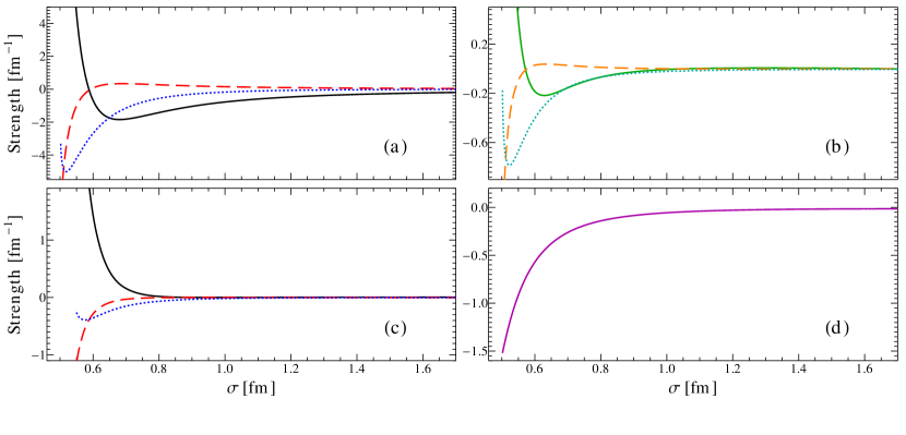
Figure 1: (Color online) Running of the parameters of the $NN$ potential as a function of the range $\sigma$. (a) $A_{1}$ (black solid curve), $A_{3}\sigma^{2}$ (red dashed curve), $A_{5}/\sigma^{2}$ (blue dotted curve). (b) $A_{2}$ (green solid curve), $A_{4}\sigma^{2}$ (orange dashed curve), $A_{6}/\sigma^{2}$ (cyan dotted curve). (c) $A_{1}^{\mathrm{CSB}}$ (black solid curve), $A_{3}^{\mathrm{CSB}}\sigma^{2}$ (red dashed curve), $A_{5}^{\mathrm{CSB}}/\sigma^{2}$ (blue dotted curve). (d) $A_{7}$ (solid magenta curve). All parameters have been multiplied with appropriate powers of $\sigma$ so that they have units of $\mathrm{fm}^{-1}$.

This unstable growth of the couplings signals the expected breakdown of this treatment when the cut-off is taken beyond the domain of validity of the EFT. For our Gaussian regulator, we can estimate the breakdown scale to be of the order of $\sigma\simeq 0.6$ fm. Noting that the Gaussian cut-off has an effective range of about $2$–$3\sigma$, this seems consistent with the scale of the underlying physics being $1/m_{\pi}$ and with the results of Scaldeferri et al. Scaldeferri:1996nx , who found a breakdown at $R\simeq 1.3$ fm for a sharp cut-off.

We therefore work with four values of $\sigma$ in our few-body calculations, namely, $\sigma=0.6,\ 0.8,\ 1.0$, and $1.2$ fm. The three larger values allow us to examine the sensitivity of our results to the choice of regulator and hence to estimate uncertainties on our results. The lowest value is there to check what happens at the breakdown point of our approach. The resulting values for the parameters $A_{i}$ and $A_{i}^{\mathrm{CSB}}$ from these fits are given in Table 1 and Table 2, respectively.

Note also that the CSB potential strengths, being very small at larger values of $\sigma$, grow even more rapidly as the range becomes shorter; indeed at $\sigma\simeq 0.6$ fm the CSB corrections become of the same size as the charge-symmetric potential. This hints at the possibility that the breakdown scale in the presence of the Coulomb interaction could be even lower than for pure short-range potentials.

Table 1: Potential strength parameters corresponding to $\sigma=0.6,\ 0.8,\ 1.0,$ and $1.2$ fm, see Eq. (3).

$\sigma$ [fm]	$A_{1}$ [fm-1]	$A_{2}$ [fm-1]	$A_{3}$ [fm-3]	$A_{4}$ [fm-3]	$A_{5}$ [fm]	$A_{6}$ [fm]	$A_{7}$ [fm-1]
$0.6$	$-0.677656$	$-0.183947$	$0.209219$	$0.078202$	$-0.967619$	$-0.144969$	$-0.571874$
$0.8$	$-1.421301$	$-0.068006$	$0.425644$	$0.017542$	$-0.355897$	$-0.044137$	$-0.140770$
$1.0$	$-0.776962$	$-0.006286$	$0.153822$	$-0.000171$	$-0.173443$	$-0.022155$	$-0.055884$
$1.2$	$-0.470719$	$0.005275$	$0.066913$	$-0.001572$	$-0.097818$	$-0.015785$	$-0.029482$

Table 2: CSB potential strength parameters corresponding to $\sigma=0.6,\ 0.8,\ 1.0,$ and $1.2$ fm, see Eq. (5).

$\sigma$ [fm]	$A_{1}^{\mathrm{CSB}}$ [fm-1]	$A_{3}^{\mathrm{CSB}}$ [fm-3]	$A_{5}^{\mathrm{CSB}}$ [fm]
$0.6$	$1.433500$	$-0.792231$	$-0.128230$
$0.8$	$0.018066$	$-0.006140$	$-0.042043$
$1.0$	$-0.000549$	$-0.000520$	$-0.017543$
$1.2$	$0.002286$	$-0.000815$	$-0.009687$

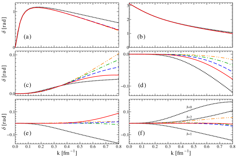
Figure 2: (Color online) Low-energy $pn$ phase shifts as described by our $NN$ potentials. The panels show the phase shifts as follows: (a) ${{}^{1}}S_{0}$; (b) ${{}^{3}}S_{1}$; (c) $\epsilon_{1}$; (d) ${{}^{3}}D_{1}$; (e) ${{}^{1}}P_{1}$; (f) ${{}^{3}}P_{0,1,2}$. Curves corresponding to the different values of $\sigma$ are: red solid: $\sigma=1.2~{}\mathrm{fm}$, blue dashed: $\sigma=1.0~{}\mathrm{fm}$, green dash-dotted: $\sigma=0.8~{}\mathrm{fm}$, orange double-dot-dashed: $\sigma=0.6~{}\mathrm{fm}$. The black dotted line shows the results of the Nijmegen PWA93 analysis Stoks:1993tb ; nn-online . Note that our calculation gives identical results for the ${{}^{3}}P_{0,1,2}$ phase shifts, see panel (f); the PWA93 curves for these phase shifts are labelled in the figure.

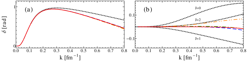
Figure 3: (Color online) Low-energy $pp$ phase shifts as described by our $NN$ potentials. The panels show the phase shifts as follows: (a) ${{}^{1}}S_{0}$; (b) ${{}^{3}}P_{0,1,2}$. The curves are denoted as in Fig. 2.

In Figs. 2 and 3 we show how closely the corresponding effective potentials reproduce the nucleon-nucleon phase shifts. The ${}^{3}S_{1}$ phase shift is reproduced very well by all four potentials. The ${}^{1}S_{0}$ phase shift is described well by our fits at low momenta, $k\lesssim 0.35~{}\mathrm{fm}^{-1}$, both in the $pn$ and in the $pp$ channel, while at larger momenta they start to deviate noticeably from the empirical values. The $S-D$ mixing angle is also reproduced rather well over this momentum range. We also show the ${{}^{3}}D_{1}$ phase shift and the $P$-wave ones (note that to this order the results for the three triplet $P$-wave phase shifts are identical, as described above). The constraints imposed on the $P$-waves mean that their phase shifts are close to zero for $k\lesssim 0.35~{}\mathrm{fm}^{-1}$, and remain much smaller than the empirical ones across the low-momentum region. The ${{}^{3}}D_{1}$ phase shift, which is not constrained, also remains smaller than the (already small) empirical shifts. Note that the plots show phases on a much bigger scale than the range of applicability of our EFT.

Table 3: Deuteron parameters resulting from the potentials with $\sigma=0.6,\ 0.8,\ 1.0,$ and $1.2$ fm, compared to experimental values.

Range $\sigma$ [fm]	Energy [MeV]	Charge radius [fm]
$0.6$	$-2.207$	$2.123$
$0.8$	$-2.207$	$2.120$
$1.0$	$-2.204$	$2.118$
$1.2$	$-2.198$	$2.116$
exp.	$-2.224$	$2.130\pm 0.010$ Sick

Table 3 shows the deuteron energy and charge radius resulting from the four selected potentials. (See Sec. V.2 for a discussion of nuclear charge radii.) As expected from the fact that these potentials describe the low-energy triplet scattering parameters very well, the results for the deuteron are very close to the experimental values. Note that the tensor potential, which is responsible for the $S-D$ mixing, is crucial for the deuteron binding (despite the mixing angle $\epsilon_{1}$ being very small). The bound state does not survive if this potential is set to zero.

V Three and four nucleons

Having determined the parameters of the two-body potentials, we now apply them to the three- and four-body nuclei. However, to do this, we first need to determine the parameters of the three-body potentials to be used in conjunction with them.

V.1 Ground-state energies

Our fitting procedure in the three- and four-nucleon sectors is as follows. First, we use the SVM to calculate the triton ground-state energy $E({{}^{3}}H)$ in an appropriate region of the plane of the three-body parameters $B_{1}$ and $B_{2}$, Eq. (9). Then, we identify those pairs of values of $B_{1}$ and $B_{2}$ that result in an energy that matches its observed value, $E({{}^{3}}H)=-8.48$ MeV. The locus of these points in the $B_{1}B_{2}$ plane is shown in Fig. 4.

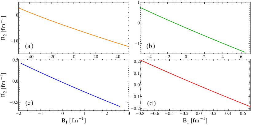
Figure 4: (Color online) Graphical representation of the relationship between the parameters $B_{1}$ and $B_{2}$ that reproduces the triton binding energy $E({{}^{3}}H)=-8.48$ MeV. Panels (a)–(d) correspond to $\sigma=0.6,\ 0.8,\ 1.0$, and $1.2$ fm, in order.

For each choice of the cut-off $\sigma$, these form almost straight lines. Another striking feature is the strong dependence of the typical sizes of these parameters on $\sigma$, with those for $\sigma=0.6$ fm being about two orders of magnitude larger than those for 1.2 fm. This is a signal that for $\sigma=0.6$ fm the expansion of our EFT is breaking down. The $\sigma=0.8$ fm potential is a borderline case: even though it does not show issues similar to those for the $\sigma=0.6$ fm potential as described below, the potential strengths show the tendency to become large already at this value of the cut-off.

The contributions, $\delta E_{B_{1}}$ and $\delta E_{B_{2}}$, of the two three-body potentials to the binding energy of ³H are shown in panel (a) of Fig. 5. It can be seen that, as a result of our use of an implicit renormalisation scheme, the contributions of these two three-body terms are of similar sizes for all potentials from the fits shown in Fig. 4. One can also see from Fig. 5 that the triton would be under-bound if only two-nucleon forces were included.

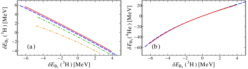
Figure 5: (Color online) (a) Correlation between the contributions of the two three-nucleon potentials, $B_{1}$ and $B_{2}$, to the triton ground-state energy for the values shown in Fig. 4. The behaviour for different values of $\sigma$ is represented by colour and line type as in Fig. 2. (b) Correlation between the contributions of $B_{1}$ to the triton and ⁴He ground-state energies. As explained in the main text, no calculation for $\sigma=0.6$ fm has been performed.

Panel (b) of Fig. 5 shows the contributions of the LO three-nucleon potential to the ³H and ⁴He binding energies. In the absence of the NLO potential, these lines would form the “Tjon lines” for our EFT Tjon:1974 . Note that they do not yet include the CSB three-body contribution in ⁴He. This figure does not show the $\sigma=0.6$ fm curve; as can be inferred from Tables 1 and 2, the CSB corrections are too big for the $\sigma=0.6$ fm potential, which expected to lead to troubles already in ³He. Furthermore, the large cancellations between the LO and NLO three-body contributions to ³H cannot be maintained in ⁴He even without the CSB corrections of Eq. (5). All this clearly signals that this cut-off is beyond the breakdown scale of the EFT; we will therefore present no further results for the $\sigma=0.6$ fm potential.

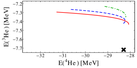
Figure 6: (Color online) Correlation between the results for the ground-state energies of ³He and ⁴He, calculated without the CSB three-nucleon force. The lines for different values of $\sigma$ are denoted as in Fig. 2. The cross marks the experimental values.

Figure 6 shows the relationship between the energies of the two helium isotopes obtained from our fitted potential, at this stage including the Coulomb and CSB nucleon-nucleon potentials but not yet the CSB three-body interaction. One can see that ³He binding energy is underestimated, whereas that of ⁴He tends to be overestimated along most of the length of the curves (even though the latter reach the experimental value at one end). The under-binding of ³He is rather small ($\sim 5\%$) but it does not depend strongly on the choice of three-body fit. In contrast the ⁴He energy varies by up to $10\%$ as the parameters are varied over the ranges shown in Fig. 4. The spread between the curves for the different values of $\sigma$ can be taken as an estimate of the uncertainties in our results due to omission of higher-order contributions. This is discussed further in Appendix B, which also contains a discussion of the numerical convergence of the SVM.

Finally we add the CSB three-nucleon interaction, fitting it to the observed ³He ground-state energy, $E({{}^{3}}\mathrm{He})=-7.718$ MeV. It is worth pointing out that this potential has a small effect on observables, in particular, the binding energy, and so, in principle, its contributions could be calculated perturbatively, by appropriately scaling the value of $B_{1}$ in the charge-symmetric ³He calculation:

$$\delta E_{\mathrm{CSB}}({{}^{3}}\mathrm{He})=\eta_{\mathrm{CSB}}\,\delta E_{B_{1}}({{}^{3}}\mathrm{He})\,,$$ (22)

where $\eta_{\mathrm{CSB}}$ is fitted to give the observed energy of ³He. With this value for $\eta_{\mathrm{CSB}}$, the contribution of the CSB interaction to ⁴He can also be estimated in the same spirit, from

$$\delta E_{\mathrm{CSB}}({{}^{4}}\mathrm{He})=\frac{1}{2}\eta_{\mathrm{CSB}}\,\delta E_{B_{1}}({{}^{4}}\mathrm{He})\,,$$ (23)

where the factor $1/2$ takes into account the symmetry of the ⁴He wave function with respect to interchange between protons and neutrons. This symmetry is only approximate since the Coulomb potential already leads to CSB at the two-nucleon level. For a precise determination of three-body CSB effects, we have used the SVM to solve Schrödinger equation with both the Coulomb potential and the CSB three-body force, using the results for ³He to determine the three-body strength $B_{\mathrm{CSB}}$. The results are within a few percent of the perturbative estimate (from $2\%$ to $4\%$ for $\sigma=1.2$ fm or $6\%$ to $9\%$ for $\sigma=0.8$ fm).

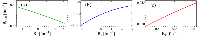
Figure 7: (Color online) Correlation of the strength $B_{\mathrm{CSB}}$ of the CSB three-nucleon potential with the value of $B_{1}$, for potentials fitted to the binding energies of ³H and ³He. Panels (a)–(c) correspond to $\sigma=0.8$, $1.0$, and $1.2$ fm, in order.

Fitting the ground-state energies of ³H and ³He leads to a one-parameter family of three-body potentials. The relationship between the strength of the CSB three-nucleon potential and that of the LO charge-symmetric potential, $B_{1}$, is shown in Fig. 7. For $\sigma=0.8$ fm and $\sigma=1.2$ fm, the correlation line is again indistinguishable from linear. For $\sigma=1.0$ fm, however, one can notice a visible deviation from straight line. This can be explained by noting that the $\sigma=0.8$ fm and the $\sigma=1.2$ fm lines have slopes of different signs; the transition from the negative to the positive slope must thus take place at some value of $\sigma$ between those two values. The $\sigma=1.0$ fm value is apparently close to that transition, therefore higher-order (quadratic) effects become visible in the corresponding curve.

This fit to both three-nucleon energies leaves only the binding energy of ⁴He as a prediction of our potentials. Including the CSB force removes the under-binding of ³He. At the same time it makes ⁴He over-bound for all our potentials: a simple combinatorial argument gives that the shift of about $-0.5$ MeV needed to correct for the under-binding of ³He translates into a shift of about $-1$ MeV in the energy of ⁴He; the latter shift will as a rule be even bigger since ⁴He is a denser system. However a single binding energy can provide only limited information on how well our EFT is describing the ground states of these light nuclei and so we now turn to calculations of their charge radii.

V.2 Charge radii

The SVM provides wave functions for the ground states of the three- and four-nucleon systems, as well as their binding energies. To test how well our EFT describes the structure of these states, we have used these wave functions to calculate charge radii. These are accessible experimentally through electron scattering Sick or isotopic shift measurements. They can be calculated by expanding the charge form factor

$$F_{C}(q^{2})=1-\frac{q^{2}r^{2}}{6}+\dots\,$$ (24)

where the $F_{C}(q^{2})$ are defined in terms of the spin-averaged matrix elements of the EM density by NED

$$F_{C}(q^{2})=\frac{1}{Z}\left\langle+\boldsymbol{q}/2\right|J^{0}_{\mathrm{em}}(\boldsymbol{q})\left|-\boldsymbol{q}/2\right\rangle\,.$$ (25)

The lowest-order coupling of the photon to the nucleon charge contributes to the form factor at $\mathcal{O}(Q^{0})$. To the order we work here, we also need operators that contribute to the form factor at two orders higher, $\mathcal{O}(Q^{2})$. The most important of these contain low-energy constants related to the charge radii of the nucleons. Two-body contributions to the charge radii appear first at $\mathcal{O}(Q^{3})$ Valderrama:2014vra , which is beyond the order considered here. As a result, we can write

$$r^{2}=\frac{1}{Z}\left\langle\Psi_{0}\right|\sum\limits_{j=1}^{A}\frac{1}{2}\left(1+\tau_{3}\right)_{j}\boldsymbol{r}_{j}^{2}\left|\Psi_{0}\right\rangle+r_{p}^{2}+\frac{3}{4M^{2}}+\frac{N}{Z}r_{n}^{2}\,,$$ (26)

where $\left|\Psi_{0}\right\rangle$ denotes the internal wave function of the ground state of the nucleus with $Z$ protons and $N=A-Z$ neutrons. Here $r_{p}=0.8751$ fm is the proton charge radius CODATA , $r_{n}^{2}=-0.1161~{}\mathrm{fm}^{2}$ is the neutron charge radius squared Kopecky:1995zz ; Kopecky:1997rw , and $3/(4M^{2})$ is the Foldy correction, which is omitted from the atomic-physics definition of the proton radius Friar:1997js .

In principle there are further relativistic recoil terms in the photon-nucleon vertex and in the nucleon propagators that are also of order $Q^{2}$. However, for the case of the deuteron it is known that these leading relativistic corrections to the charge radius are numerically very small Chen:1999tn . On dimensional grounds, the corrections to Eq. (26) must scale as $C/M^{2}$, where $C$ is a constant. If one takes $C$ to be of the order of one (and it is much smaller than that for the deuteron), these corrections result in shifts of less than $\pm 0.01$ fm in the values of the charge radii. We have also calculated some of these corrections for terms that stem from $1/M^{2}$ recoil corrections to the photon-nucleon vertex. We find that these make very small contributions to the nuclear charge radii, about $0.003$ fm for ⁴He and even less for the three-nucleon systems.

With the wave functions from the SVM, it is straightforward to evaluate Eq. (26) for the charge radii. The results are shown in Table 3 for the deuteron and in Fig. 8 for ³H, ³He, and ⁴He. In the case of the deuteron, they agree with the experimental value to better than $1\%$ for all four choices of regulator.

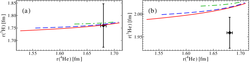
Figure 8: (Color online) (a): Correlation between ⁴He and ³H charge radii; (b): Correlation between ⁴He and ³He charge radii. The lines for different values of $\sigma$ are denoted as in Fig. 2. The experimental values are taken from Ref. Sick .

The results in Fig. 8 show that all families of three-body potentials are in remarkably good agreement with the experimental value for the ³H charge radius. The values for the charge radius of ³He are somewhat larger than the experimental one, but the discrepancy is never more than two standard deviations. The significance of the differences is further reduced if we take account of the theoretical uncertainties in our results, as indicated by the spread between the curves. It may also be worth noting that taking the value for the proton charge radius obtained from muonic hydrogen Antognini:1900ns , $r_{p}=0.8409$ fm, would shift the ³He results down to within $1.5$ standard deviations of the experimental value. Another interesting feature is that the three-nucleon CSB force that compensates for the under-binding of ³He is also quite important for the description of the ³He charge radius; without this force we would get larger radii (as expected), the typical values being about $2.05$ fm.

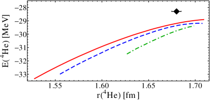
Figure 9: (Color online) Correlation between ⁴He charge radius and ground state energy. The notation is as in Fig. 4.

Finally, in Fig. 9, we present our results for the energy and the charge radius of ⁴He for our families of three-body potentials. For each family, the charge radius shows the expected correlation with energy, decreasing with increasing binding energy, as expected. As already mentioned, ⁴He is still over-bound, by about $1..1.5$ MeV for potentials that reproduce the observed charge radius. This difference is small (about $3\%$ to $5~{}\%$ of the binding energy) and within the expected truncation error of the EFT expansion.

As discussed further in Appendix B, we estimate the uncertainty from the spread of the results for different choices of cut-off. For the potentials that describe all four observables, this spread is typically about $3\%$, which is consistent with the expected error due to our truncation of the EFT at NNLO, which is $\sim(1/3)^{3}$ for an expansion parameter which we estimate to be $Q\simeq 1/3$.

VI Discussion

In this work we have studied nuclei with $A=3$ and $4$ in the framework of the pionless EFT, working at NNLO. We use a Hamiltonian formulation rather than the more usual Lagrangian version, expressing the interactions in the form of local potentials with a Gaussian regulator. As well as short-range two- and three-body forces, we also include the Coulomb potential. To the order we work, this also requires that we add CSB two- and three-body contact interactions.

The resulting Schrödinger equation is solved variationally using the SVM with a basis of Gaussian trial functions. This provides ground-state energies and wave functions for the nuclei with $A=3$ and $4$. Since our three-body potential contains three terms, fitting the energies of ³H and ³He leaves us with a one-parameter family of potential for each choice of cut-off.

In this approach, the whole potential is treated to all orders. This means that we cannot renormalise it perturbatively; instead we use an implicit renormalisation. If the regulator scale is taken above the breakdown scale of the EFT, this can lead to very large values for the parameters with extreme fine-tuning in order to reproduce observables. We find that the determination of parameters becomes unstable for potential with ranges $\sigma<0.8\text{ fm}$. Moreover, the higher-order effects of these fine-tuned potentials are large for nuclei with $A>2$, and thus the results for binding energies are actually quite poor. We therefore reject these unnatural solutions.

For each of these potentials we have calculated the binding energy of ⁴He and the charge radii of the nuclei with $A=3$ and $4$. The dependence of the results on the cut-off provides a measure of the uncertainties in our results. These are about $3\%$, which matches what we expect for our truncation of the EFT. We see some indications that the agreement with empirical data for $A=4$ is slightly poorer than for $A=3$, which is not a surprise given that ⁴He is a denser system, with higher typical momenta.

Within these uncertainties and those of the data, we are able to find potentials that give good agreement with the measured values of the ⁴He energy and the charge radii.

In this paper we have concentrated on the specific form of the interaction that applies to the (almost) Wigner-$\mathrm{SU}(4)$-symmetric $A\leq 4$ nuclei. Extending our method to mixed-symmetry nuclei with $A>4$ will require determination of many more parameters. A natural way to do this is through fitting scattering observables. This will require an extension of SVM using, for example, the Kohn variational principle.

Appendix A Kohn variational principle

In order to construct a low-energy nucleon-nucleon potential, we employ the complex variant of the Kohn variational method (see Refs. Miller1987 ; McCurdy1987 ; Schneider:1988zz ). The idea of this method is based on the fact that the Lippmann-Schwinger equation for the scattering operator $T$,

$$T(E)=V+VG^{(+)}(E)V\,,$$ (27)

can be recast into the problem of finding the stationary point of a functional involving either $T$ or the exact Green’s function with the outgoing-wave (radiation) boundary condition,

$$G^{(+)}(E)=\left[E-H+i0\right]^{-1}\,.$$ (28)

For a particular choice of the trial wave functions (see the above cited references for further details of the derivation which we omit), the resulting variational expression for the Green’s function projected onto partial waves reads:

$$G^{(+)}(r^{\prime},r)=\sum\limits_{i,j}\phi_{i}(r^{\prime})\left[\mathsf{E}-\mathsf{H}\right]^{-1}_{ij}\phi_{j}(r)\,,$$ (29)

where the matrix $\left[\mathsf{E}-\mathsf{H}\right]^{-1}$ is the inverse of the square matrix with entries $\left\langle\phi_{i}^{*}\right|\left[E-H\right]\left|\phi_{j}\right\rangle$. The radiation condition is carried by one of the wave functions, and the remainder remains finite and is square-integrable,

$$\begin{split}&\phi_{0}(r)\propto\frac{e^{ikr}}{r},\quad r\to\infty\,,\\ &\phi_{j}(r)\to 0,\quad r\to\infty\,,\ j>0\,,\\ &\phi_{j}(r)\propto r^{l},\quad r\to 0\,,\ j>0\,,\end{split}$$ (30)

with $k=\sqrt{ME}$ being the relative momentum and $l$ the angular momentum in the corresponding partial wave. Note that the vectors $\phi(r^{\prime})$ in Eq. (29) are not complex conjugated as one would naively expect; this follows from the radiation condition on the Green’s function Miller1987 .

As long as the basis functions satisfy the conditions given by Eq. 30, one can select them based on convenience of use in the particular calculation. The basis used by us is given by

$$\begin{split}&r\phi_{0}(r)=ik^{l+1}r\left(1-e^{-r/\alpha_{0}}\right)^{2l+1}h^{(+)}_{l}(kr)\,,\\ &r\phi_{j}(r)=\sqrt{\frac{2(j-1)!}{\alpha(j+2l-1)!}}\left(2r/\alpha\right)^{l+1}e^{-r/\alpha}L^{(2l+2)}_{j-1}(2r/\alpha)\,,\ j>0\,,\end{split}$$ (31)

where $h^{(+)}_{l}(x)$ is the spherical Hankel function of the first kind, $L^{(2l+2)}_{j}(x)$ are the associated Laguerre polynomials, and $\alpha_{0}$ and $\alpha$ are real parameters that can be fine-tuned so as to improve the convergence of the calculation. The results shown in this work were obtained with $\alpha_{0}=1$ fm, $\alpha=0.25$ fm. The free solutions to the wave equation are the spherical Bessel functions,

$$\psi_{l}(k,r)=j_{l}(kr)\,.$$ (32)

With this normalisation, the matrix elements of the scattering operator (27) are just minus the scattering amplitude between the corresponding partial waves:

$$f_{ll^{\prime}}(k)=-\left\langle\psi_{l}\right|V\left|\psi_{l^{\prime}}\right\rangle-\left\langle\psi_{l}\right|VG^{(+)}(E)V\left|\psi_{l^{\prime}}\right\rangle\,.$$ (33)

Equations (31–33) can be used to extract the nucleon-nucleon scattering parameters such as scattering lengths and effective ranges resulting from the specific potential $V$, and thus allow for fitting the parameters of the potential.

Proton-proton scattering can also be treated by this method, using a distorted-wave formulation Miller1987 . Namely, the radiation condition of Eq. (30) needs to be replaced by the Coulomb radiation condition:

$$\begin{split}&\phi_{0}(r)\propto\frac{e^{i\left(kr-\eta\ln 2kr+\delta_{l}\right)}}{r},\quad r\to\infty\,,\\ \end{split}$$ (34)

where

$$\eta=\frac{M\alpha_{\mathrm{em}}}{2k},\quad\delta_{l}=\operatorname{Arg}\Gamma(1+l+i\eta)\,.$$ (35)

The Coulomb-modified basis functions that we use are

$$\begin{split}&r\phi_{0}(r)=(-ik)^{l}e^{\pi\eta/2+i\delta_{l}}\left(1-e^{-r/\alpha_{0}}\right)^{2l+1}W_{-i\eta,l+1/2}(-2ikr)\,,\\ \end{split}$$ (36)

with $\phi_{j}(r)$ given by Eq. (31) for $j>0$, with the same values of $\alpha_{0}$ and $\alpha$. The free spherical Bessel functions, in turn, are replaced by the regular solutions to the Coulomb equation:

$$\psi^{C}_{l}(k,r)=\frac{C_{l}}{kr}(-i/2)^{l+1}M_{i\eta,l+1/2}(2ikr)\,,$$ (37)

where

$$C_{l}=\frac{2^{l}e^{-\pi\eta/2}\left|\Gamma(1+l+i\eta)\right|}{(2l+1)!}\,.$$ (38)

Here, $W_{a,b}(z)$ and $M_{a,b}(z)$ are the Whittaker functions (for details see, e.g., Refs. (dlmf, , Chapters 13, 33) and (Messiah, , Appendix B)). With these definitions, the strong scattering amplitude in the presence of the Coulomb interaction is given by

$$f_{ll^{\prime}}(k)=-\left\langle\psi^{C}_{l}\right|V\left|\psi^{C}_{l^{\prime}}\right\rangle-\left\langle\psi^{C}_{l}\right|VG^{(+)}(E)V\left|\psi^{C}_{l^{\prime}}\right\rangle\,,$$ (39)

where $V$ is now only the strong part of the potential, whereas $G^{(+)}(E)$ is the full Green’s function constructed as given by Eq. (29) with the full (strong $+$ Coulomb) potential.

Appendix B Convergence

B.1 Numerical convergence of the SVM

As a variational method, the SVM gives upper bounds for the energy eigenvalues, with each consecutive expansion of the basis, i.e., addition of a new trial function, lowering the energies Suzuki:1998bn . After having diagonalised the Hamiltonian for $m$ basis states, the $(m+1)^{\mathrm{th}}$ trial state is selected without solving the complete generalised eigenvalue problem (18). Only once this state is selected, the generalised eigenvalue problem is solved in the $m+1$-dimensional basis. When the basis size is very large, the energy gain achieved thanks to expanding it further from $m$ to $m+1$ functions can become smaller than the numerical error of the solution of the eigenvalue problem, usually indicating no further gain can be made.

We find that convergence with respect to the size of the basis is typically faster for smoother (longer-range) potentials, as well as for smaller systems. This can also be seen in the saturation of the basis mentioned above; this also occurs faster in smoother potentials and in smaller systems. Table 4 lists the bases sizes $m_{\mathrm{max}}$ used in this work, together with an estimate of the change in energy achievable by extending the basis size to infinity. These estimates are obtained by fitting the tail of the dependence of the lowest eigenvalue of (18) by a linear function in the reciprocal basis size $1/m$, $E_{0}(m)=E_{0}^{\mathrm{lim}}+\Delta E_{0}/m$. We used the values of $E_{0}(m)$ with $m>250$ for $A=3$ systems, and $m>400$ for $A=4$. The uncertainty estimate is then given by $\delta E_{0}=\left|E_{0}^{\mathrm{lim}}-E_{0}(m_{\mathrm{max}})\right|$. The quoted values are the maximal uncertainties for each potential.

Table 4: Basis sizes for $A=3$ and $4$ calculations used in this work and estimated uncertainties of the ground state energies.

	3H, 3He		4He
$\sigma$ [fm]	$m_{\mathrm{max}}$	$\delta E_{0}$[MeV]	$m_{\mathrm{max}}$	$\delta E_{0}$[MeV]
$0.8$	$500$	$0.03$	$1200$	$0.11$
$1.0$	$500$	$0.03$	$750$	$0.18$
$1.2$	$450$	$0.02$	$750$	$0.07$

B.2 Convergence of the EFT expansion

The method employed in this paper makes it harder to judge the convergence of the EFT series than it would be in a treatment based on a strict perturbation theory approach. The use of finite cut-off to regularise the Schrödinger equation, together with implicit renormalisation, means that there is no clean separation between orders, powers of $Q$, at the level of the potential. Nevertheless, one would expect that the changes in observables decrease as one includes terms that contain higher and higher pieces in the expansion of the potential. In addition, the dependence of the results on the regulator parameter $\sigma$, such as that in Figs. 8–9, can provide an estimate of the size of higher-order corrections.

In Table 5 we show a breakdown of the energies of the $A=2$, $3$ and $4$ systems into contributions of the various terms in the two- and three-nucleon potentials, Eqs. (3)-(5), (9), and (12). The first row again illustrates the problems that arise when using a regulator with too short a range. Although the $\sigma=0.6$ fm potential reproduces the nucleon-nucleon phase shifts and the deuteron binding energy with the same quality as the other three potentials, it gets its largest contribution to the binding of the deuteron from the tensor interaction. That interaction, although nominally of NNLO, is by far the most important at this scale, which clearly shows that one cannot keep higher-order effects under control when the cut-off is too short-ranged.

Table 5: Contributions to the ground-state energies of the deuteron, ³H, ³He, and ⁴He, from different components of the interaction are shown in Table 5. The column labelled $E$ contains the ground-energies; the one labelled $T$, the sums of the corresponding kinetic and Coulomb energies. The labels $A_{1\dots 7}$, $B_{1,2}$, and $B_{\mathrm{CSB}}$ indicate the contributions of those interactions to the energies. All quantities are in units of MeV (except $\sigma$). The three-body and four-body energies are given for the values of three-body parameters that reproduce the observed ⁴He charge radius ($1.680$ fm).

Deuteron
$\sigma$[fm]	$E$	$T$	$A_{1}$	$A_{2}$	$A_{3}$	$A_{4}$	$A_{5}$	$A_{6}$	$A_{7}$	$B_{1}$	$B_{2}$	$B_{\mathrm{CSB}}$
$0.6$	$-2.21$	$15.41$	$-5.13$	$4.18$	$1.72$	$-1.93$	$9.65$	$-4.33$	$-21.76$	$-$	$-$	$-$
$0.8$	$-2.21$	$12.90$	$-27.46$	$3.94$	$11.55$	$-1.42$	$13.28$	$-4.94$	$-10.05$	$-$	$-$	$-$
$1.0$	$-2.20$	$12.18$	$-24.51$	$0.60$	$8.88$	$0.03$	$9.70$	$-3.71$	$-5.36$	$-$	$-$	$-$
$1.2$	$-2.20$	$11.80$	$-20.37$	$-0.69$	$6.69$	$0.47$	$6.57$	$-3.17$	$-3.49$	$-$	$-$	$-$
3H
$0.8$	$-8.48$	$30.18$	$-85.43$	$6.13$	$38.14$	$-2.09$	$32.48$	$-8.87$	$-18.04$	$0.39$	$-1.36$	$0$
$1.0$	$-8.48$	$28.74$	$-79.59$	$0.89$	$30.61$	$0.04$	$26.83$	$-6.26$	$-9.32$	$1.57$	$-1.99$	$0$
$1.2$	$-8.48$	$28.21$	$-67.99$	$-1.00$	$23.40$	$0.62$	$19.71$	$-5.31$	$-5.96$	$1.31$	$-1.46$	$0$
3He
$0.8$	$-7.72$	$24.47$	$-63.40$	$7.10$	$27.18$	$-2.51$	$28.11$	$-9.40$	$-17.92$	$0.37$	$-1.28$	$-0.44$
$1.0$	$-7.72$	$22.86$	$-57.39$	$1.05$	$21.20$	$0.05$	$21.40$	$-6.89$	$-9.25$	$1.50$	$-1.90$	$-0.36$
$1.2$	$-7.72$	$22.19$	$-48.23$	$-1.20$	$15.94$	$0.79$	$15.16$	$-5.97$	$-5.91$	$1.25$	$-1.40$	$-0.33$
4He
$0.8$	$-29.74$	$55.22$	$-192.63$	$15.40$	$82.55$	$-5.23$	$82.06$	$-21.64$	$-37.53$	$2.63$	$-8.99$	$-1.57$
$1.0$	$-29.36$	$50.64$	$-171.82$	$2.30$	$63.12$	$0.10$	$63.30$	$-15.04$	$-18.33$	$9.72$	$-12.11$	$-1.15$
$1.2$	$-29.19$	$49.15$	$-143.97$	$-2.49$	$46.28$	$1.55$	$46.41$	$-13.07$	$-11.33$	$7.94$	$-8.63$	$-1.04$

For the other three values of the cut-off that we considered, the two-body contributions to the ground state energies do indeed decrease with increasing order of the potential. The ratio between NLO and LO contributions, as well as that between NNLO and NLO ones, is roughly $1/3$. This provides a concrete estimate of our expansion parameter $Q$. Higher-order corrections to our NNLO results are therefore expected to be of the order of $Q^{3}\simeq 3\%$. This estimate is confirmed by the spread between the values of, for example, the binding energy of ⁴He for different values of $\sigma$. This regulator dependence is also at the level of about $3\%$, cf. Fig. 9. The similarity between this dependence and the expected size of the higher-order contributions suggests that the higher-order terms are also under control for this range of cut-offs.

The three-nucleon forces, although formally of LO, give rather small contributions to three- and four-nucleon ground-state energies. This is consistent with what was observed long ago in phenomenological models (see, for example, Ref. Wiringa:2002ja ). In an EFT, however, the three-body forces serve not only to reproduce the three-body binding energies, but also to renormalise the latter or, in our approach, to cancel the regulator dependence of certain observables. Since the LO and NLO three-nucleon potentials are fitted to reproduce the ³H ground-state energy, one cannot use the latter observable to judge the regulator dependence. However, one can use other three-body observables such as the ³H and ³He charge radii. As shown in Fig. 8, the cut-off dependence of the three-body charge radii is numerically smaller than the expected $3\%$ spread, especially in the case of ³H. This indicates that the wave functions obtained for the combination of the LO and NLO three-nucleon forces fixed by fitting the ³H ground-state energy give consistent results for other three-body observables.

One can also see a mismatch between the sizes of the LO and NNLO three-nucleon potential contributions in Table 5 (the $B_{1}$ and $B_{2}$ terms): the subleading contribution is sometimes larger than the leading one, especially for the shortest-range potential. Nonetheless, the total contribution from these interactions seems to be well under control.

Finally, the CSB three-nucleon force, Eq. (12), which is fitted so as to reproduce ³He binding energy, gives a very small contribution to the ground-state energies (except in the case of $\sigma=0.8$ fm). One would also expect this contribution to be larger in ⁴He than in ³He, as the former nucleus is more dense. The numbers in Table 5 confirm this expectation.

Our analysis of the contributions at different orders thus suggests a value of the expansion parameter $Q\simeq 1/3$, which translates to an accuracy of about $3\%$ for our NNLO calculation. This estimate is compatible with the apparent mismatch between our result and the observed ⁴He ground-state energy. It is also consistent with the spread between the values of this energy obtained for choices of the regulator scale $\sigma$, which is also at the level of $3$–$5\%$. Three-body observables, such as the ³H and ³He charge radii, show even better agreement with empirical data, which is as expected since the three-nucleon potential strengths are fitted to the triton ground-state energy. CSB interactions, such as the NNLO CSB three-nucleon force, make rather small contributions, but are important in order to obtain a satisfactory description of the data.

References

- (1) S. Weinberg, Phys. Lett. B 251 (1990) 288.
- (2) S. Weinberg, Nucl. Phys. B 363 (1991) 3.
- (3) D. B. Kaplan, M. J. Savage and M. B. Wise, Phys. Lett. B 424 (1998) 390; Nucl. Phys. B 534 (1998) 329.
- (4) P. F. Bedaque and U. van Kolck, Annu. Rev. Nucl. Part. Sci. 52 (2002) 339 arXiv:nucl-th/0203055.
- (5) J. W. Chen, G. Rupak and M. J. Savage, Nucl. Phys. A 653 (1999) 386 arXiv:nucl-th/9902056.
- (6) H. A. Bethe, Phys. Rev. 76 (1949) 38.
- (7) P. F. Bedaque, H.-W. Hammer and U. van Kolck, Phys. Rev. Lett. 82 (1999) 463 arXiv:nucl-th/9809025.
- (8) G. V. Skorniakov and K. A. Ter-Martirosian, Zh. Eksp. Teor. Fiz. 31, 775 (1956) [Sov. Phys. JETP 4, 648 (1957)].
- (9) J. Vanasse, arXiv:1512.03805 [nucl-th].
- (10) L. Platter, H.-W. Hammer and U.-G. Meißner, Phys. Lett. B 607 (2005) 254 arXiv:nucl-th/0409040.
- (11) J. Kirscher, H. W. Grießhammer, D. Shukla and H. M. Hofmann, Eur. Phys. J. A 44 (2010) 239 arXiv:0903.5538 [nucl-th].
- (12) Y. C. Tang, M. Lemere and D. R. Thompson, Phys. Rept. 47 (1978) 167.
- (13) H. M. Hofmann, in Proceedings of Models and Methods in Few-Body Physics, Lisbon, Portugal 1986, Lecture Notes in Physics Vol. 273, edited by L. S. Ferreira, A. C. Fonseca, and L. Streit (Springer, New York, 1987), p. 243.
- (14) A. Kievsky, S. Rosati, M. Viviani, L. E. Marcucci and L. Girlanda, J. Phys. G 35 (2008) 063101 arXiv:0805:4688 [nucl-th].
- (15) Y. Suzuki and K. Varga, Lecture Notes in Physics Monographs Vol. 54, (Springer, Berlin Heidelberg, 1998).
- (16) S. König, H. W. Grießhammer, H.-W. Hammer and U. van Kolck, J. Phys. G 43 (2016) 055106 arXiv:1508.05085 [nucl-th].
- (17) E. Epelbaum and J. Gegelia, Eur. Phys. J. A 41 (2009) 341 arXiv:0906.3822 [nucl-th].
- (18) M. C. Birse, PoS CD 09 (2009) 078 arXiv:0909.4641 [nucl-th].
- (19) X. Kong and F. Ravndal, Phys. Lett. B 450 (1999) 320 arXiv:nucl-th/9811076.
- (20) X. Kong and F. Ravndal, Nucl. Phys. A 665 (2000) 137 arXiv:hep-ph/9903523.
- (21) J. Vanasse, D. A. Egolf, J. Kerin, S. König and R. P. Springer, Phys. Rev. C 89 (2014) 064003 arXiv:1402.5441 [nucl-th].
- (22) C. Ordonez, L. Ray and U. van Kolck, Phys. Rev. C 53 (1996) 2086 arXiv:hep-ph/9511380.
- (23) M. C. Birse, J. A. McGovern and K. G. Richardson, Phys. Lett. B 464 (1999) 169 arXiv:hep-ph/9807302.
- (24) A. Gezerlis, I. Tews, E. Epelbaum, M. Freunek, S. Gandolfi, K. Hebeler, A. Nogga and A. Schwenk, Phys. Rev. C 90 (2014) 054323 arXiv:1406.0454 [nucl-th].
- (25) M. M. Nagels, T. A. Rijken and J. J. de Swart, Phys. Rev. D 17 (1978) 768.
- (26) S. Ando and M. C. Birse, J. Phys. G 37 (2010) 105108 arXiv:1003.4383 [nucl-th].
- (27) G. Rupak and X. Kong, Nucl. Phys. A 717 (2003) 73 arXiv:nucl-th/0108059.
- (28) J. Gasser and H. Leutwyler, Phys. Rep. 87 (1982) 77.
- (29) K. A. Scaldeferri, D. R. Phillips, C. W. Kao and T. D. Cohen, Phys. Rev. C 56 (1997) 679 arXiv:nucl-th/9610049.
- (30) D. R. Phillips and T. D. Cohen, Phys. Lett. B 390 (1997) 7 arXiv:nucl-th/9607048.
- (31) J. Kirscher and D. Gazit, Phys. Lett. B 755 (2016) 253.
- (32) V. Efimov, Phys. Lett. B 33 (1970) 563.
- (33) T. Barford and M. C. Birse, J. Phys. A 38 (2005) 697 arXiv:nucl-th/0406008.
- (34) P. F. Bedaque, G. Rupak, H. W. Grießhammer and H.-W. Hammer, Nucl. Phys. A 714 (2003) 589 arXiv:nucl-th/0207034.
- (35) E. Epelbaum, A. Nogga, W. Glöckle, H. Kamada, U.-G. Meißner and H. Witala, Phys. Rev. C 66 (2002) 064001 arXiv:nucl-th/0208023.
- (36) L. Girlanda, A. Kievsky and M. Viviani, Phys. Rev. C 84 (2011) 014001 arXiv:1102.4799 [nucl-th].
- (37) H. W. Grießhammer, Nucl. Phys. A 760 (2005) 110 arXiv:nucl-th/0502039.
- (38) J. E. Lynn, I. Tews, J. Carlson, S. Gandolfi, A. Gezerlis, K. E. Schmidt and A. Schwenk, Phys. Rev. Lett. 116 (2016) 062501 arXiv:1509.03470 [nucl-th].
- (39) W. H. Miller and B. M. D. D. Jansen op de Haar, J. Chem. Phys. 86, 6213 (1987).
- (40) C. W. McCurdy, T. N. Rescigno, and B. I. Schneider, Phys. Rev. A 36 (1987) 2061.
- (41) B. I. Schneider and T. N. Rescigno, Phys. Rev. A 37 (1988) 3749.
- (42) R. B. Wiringa, V. G. J. Stoks and R. Schiavilla, Phys. Rev. C 51 (1995) 38 arXiv:nucl-th/9408016.
- (43) V. G. J. Stoks, R. A. M. Klomp, M. C. M. Rentmeester and J. J. de Swart, Phys. Rev. C 48 (1993) 792.
- (44) NN-Online, http://nn-online.org
- (45) I. Sick, in Precision Physics of Simple Atoms and Molecules, edited by S. G. Karshenboim, Lecture Notes in Physics Vol. 745 (Springer, Berlin Heidelberg, 2008), p. 57.
- (46) J. A. Tjon, Phys. Lett. B 56 (1975) 217.
- (47) A. Akhiezer, A. Sitenko, and V. Tartakovskii, Nuclear Electrodynamics, Springer Series in Nuclear and Particle Physics (Springer, New York, 1994).
- (48) M. P. Valderrama and D. R. Phillips, Phys. Rev. Lett. 114 (2015) 082502 arXiv:1407.0437 [nucl-th].
- (49) P. J. Mohr, D. B. Newell, B. N. Taylor, arXiv:1507.07956 [physics:atom-ph].
- (50) S. Kopecky, P. Riehs, J. A. Harvey and N. W. Hill, Phys. Rev. Lett. 74 (1995) 2427.
- (51) S. Kopecky, M. Krenn, P. Riehs, S. Steiner, J. A. Harvey, N. W. Hill and M. Pernicka, Phys. Rev. C 56 (1997) 2229.
- (52) J. L. Friar, J. Martorell and D. W. L. Sprung, Phys. Rev. A 56 (1997) 4579.
- (53) A. Antognini et al., Science 339 (2013) 417.
- (54) NIST Digital Library of Mathematical Functions, http://dlmf.nist.gov, release 1.0.10 of 2015-08-07.
- (55) A. M. L. Messiah, Quantum Mechanics (John Wiley and Sons, New York, 1961).
- (56) R. B. Wiringa and S. C. Pieper, Phys. Rev. Lett. 89 (2002) 182501 arXiv:nucl-th/0207050.