Poincaé type inequalities for vector functions with zero mean normal traces on the boundary and applications to interpolation methods

Abstract.

In the paper, we consider inequalities of the Poincaré–Steklov type for subspaces of $H^{1}$-functions defined in a bounded domain $\Omega\in\mathbb{R}^{d}$ with Lipschitz boundary $\partial\Omega$. For scalar valued functions, the subspaces are defined by zero mean condition on $\partial\Omega$ or on a part of $\partial\Omega$ having positive $d-1$ measure. For vector valued functions, zero mean conditions are imposed on components (e.g., normal components) of the function on certain $d-1$ dimensional manifolds (e.g., on plane or curvilinear faces of $\partial\Omega$). We find explicit and simply computable bounds of the respective constants for domains typically used in finite element methods (triangles, quadrilaterals, tetrahedrons, prisms, pyramids, and domains composed of them). The second part of the paper discusses applications of the estimates to interpolation of scalar and vector valued functions.

1. Introduction

1.1. Classical Poincaré inequality

H. Poincaré [22] proved that $L^{2}$ norms of functions with zero mean defined in a bounded domain $\Omega$ with smooth boundary $\partial\Omega$ are uniformly bounded by the $L^{2}$ norm of the gradient, i.e.,

(1.1) $$\|w\|_{2,\Omega}\leq C_{\rm P}(\Omega)\|\nabla w\|_{2,\Omega},\qquad\forall w\in\widetilde{H}^{1}(\Omega),$$

where

$$\widetilde{H}^{1}(\Omega):=\left\{w\in H^{1}(\Omega)\,\mid\,\left\{\!\!\left|\,w\,\right|\!\!\right\}_{\Omega}:=\frac{1}{|\Omega|}\int\limits_{\Omega}w\,dx=0\right\}.$$

Poincaré also deduced the very first estimates of $C_{\rm P}$:

(1.2) $$C_{\rm P}(\Omega)\leq\frac{3}{4}{\rm d}_{\Omega},\quad{\rm d}_{\Omega}:={\rm diam}\,\Omega\quad {\rm for}\;d=3\;$$

(1.3) $$\;C_{\rm P}(\Omega)\leq\,\sqrt{\frac{7}{24}}{\rm d}_{\Omega}\approx 0.5401{\rm d}_{\Omega}\quad {\rm for}\;d=2.$$

For piecewise smooth domains the inequality (1.1) (and a similar inequality for functions vanishing on the boundary) was independently established by V. Steklov [28], who proved that $C_{\rm P}=\lambda^{-\frac{1}{2}}$, where $\lambda$ is the smallest positive eigenvalue of the problem

(1.4) $$-\Delta u={\lambda}u \mbox{in}\quad\Omega;$$

(1.5) $$\partial_{{\bf n}}u=0 \mbox{on}\quad\partial\Omega.$$

Easily computable estimates of $C_{\rm P}(\Omega)$ are known for convex domains in $\mathbb{R}^{d}$. An upper bound

(1.6) $$\;C_{\rm P}(\Omega)\,\leq\,\frac{{\rm d}_{\Omega}}{\pi}\;\approx 0.3183\,{\rm d}_{\Omega}$$

was established in L. E. Payne and H. F. Weinberger [23] (notice that for $d=2$ the upper bound (1.3) found by Poincar e is not far from the sharp estimate (1.6)).

A lower bound of $C_{\rm P}(\Omega)$ was derived in S. Y. Cheng [6] (for $d=2$):

(1.7) $$C_{\rm P}(\Omega)\geq\,\frac{{\rm d}_{\Omega}}{2j_{0,1}}\;\approx 0.2079\,{\rm d}_{\Omega}.$$

Here $j_{0,1}\approx 2.4048$ is the smallest positive root of the Bessel function $J_{0}$.

For isosceles triangles an improvement of the upper bound (1.6) is presented in R. S. Laugesen and B. A. Siudeja [17]

(1.8) $$C_{\rm P}(\Omega)\leq\,\frac{d_{\Omega}}{j_{1,1}},$$

where $j_{1,1}\approx 3.8317$ is the smallest positive root of the Bessel function $J_{1}$.

Poincaré type inequalities also hold for $L^{q}$ norms if $1\leq q<+\infty$. In G. Acosta and R. Duran (2003), it was shown that for convex domains the constant in $L_{1}$ Poincaré type inequality satisfies the estimate

(1.9) $$\inf_{c\in{\mathbb{R}}}\|w-c\|_{L_{1}}\leq\frac{{\rm d}_{\Omega}}{2}\|\nabla w\|_{L_{1}}.$$

Estimates of the constant for other $q$ can be found in S.-K. Shua and R. L. Wheeden (2006) (also for convex domains).

1.2. Poincaré type inequalities for functions with zero mean boundary traces

Inequalities similar to (1.1) also hold for functions with zero mean traces on the boundary (or on a measurable part $\Gamma\subset\partial\Omega$) such that ${\rm meas}_{(d-1)}\Gamma>0$. For any

$$w\,\in\,\widetilde{H}^{1}_{\Gamma}(\Omega)=\Bigl{\{}w\in H^{1}(\Omega)\,\Bigl{|}\Bigr{.}\,\left\{\!\!\left|\,w\,\right|\!\!\right\}_{\Gamma}:=\frac{1}{|\Gamma|}\int\limits_{\Gamma}w\,ds=0\Bigr{\}},$$

we have two estimates for the $L^{2}(\Omega)$ norm of $w$

(1.10) $$\|w\|_{2,\Omega}\leq\;C_{\Gamma}(\Omega)\|\nabla w\|_{2,\Omega}$$

and and for its trace on the $\Gamma$

(1.11) $$\|w\|_{2,\Gamma}\leq\;C^{\rm Tr}_{\Gamma}(\Omega)\|\nabla w\|_{2,\Omega}.$$

Existence of positive constants $C_{\Gamma}(\Omega)$ and $C^{\rm Tr}_{\Gamma}(\Omega)$ is proved by standard compactness arguments. Inequality (1.10) arises in analysis of certain physical phenomena (the so called ”sloshing” frequencies, see D. W. Fox and J. R. Kuttler [8], V. Kozlov et al. [9, 10] and references therein). In the paper by I. Babuska and A. K. Aziz [3] it was used in proving sufficiency of the maximal angle condition for finite element meshes with triangular elements. Inequalities (1.10) and (1.11) can be useful in many other cases, e.g., for nonconforming approximations, a posteriori error estimates (see [19, 26, 18, 24]), and and advanced interpolation methods for scalar and vector valued functions. In this paper, we are mainly interested in the inequality (1.10) for functions with zero mean on $\Gamma$. For the sake of brevity, we will call it the boundary Poincaré inequality.

Exact constants $C_{\Gamma}$ and $C^{\rm Tr}_{\Gamma}$ are known only for a restricted number of ”simple” domains. Table 1 summarises some of the results presented in A. Nazarov and S. Repin [21], which are related to such domains as rectangle $\Pi_{h1\times h_{2}}:=(0,h_{1})\times(0,h_{2})$, parallelepiped $\Pi_{h1\times h_{2}\times h_{3}}:=(0,h_{1})\times(0,h_{2})\times(0,h_{3})$, and right triangle $\overline{T}_{h}:={\rm conv}\{(0,0),(h,0),(0,h)\}$.

$d$	$\Omega$	$\Gamma$	$C_{\Gamma}(\Omega)$
$2$	$\Pi_{h1\times h_{2}}$	face $x_{1}=0$	$c_{1}\max\{2h_{1};h_{2}\}$, $c_{1}=1/\pi$
$2$	$\Pi_{h1\times h_{2}}$	$\partial\Omega$	$c_{1}\max\{h_{1};h_{2}\}$
$3$	$\Pi_{h1\times h_{2}\times h_{3}}$	face $x_{1}=0$	$c_{1}\max\{2h_{1};h_{2};h_{3}\}$
$2$	$T_{h}$	leg	$c_{2}h$,  $c_{2}=1/\zeta$,  $\scriptstyle\zeta\approx 2.02876$
$2$	$T_{h}$	two legs	$c_{1}h$
$2$	$T_{h}$	hypothenuse	$\sqrt{2}c_{2}h$

Table 1. Sharp constants

In Section 2 we deduce easily computable majorants of $C_{\Gamma}$ for triangles, rectangles, tetrahedrons, polyhedrons, pyramides and prizmatic type domains. These results yield interpolation estimates (and respective constants) for interpolation of scalar valued functions on macrocells based on mean values on faces. As a result, we can deduce interpolation estimates for functions defined on meshes with very complicated (e.g., nonconvex) cells.

Section 3 is concerned with boundary Poincaré inequalities for vector valued functions. Certainly, (1.10) admits a straightforward extension to vector fields. We consider more sophisticated forms where zero mean conditions are imposed on mean values of different components of a vector valued function ${\bf v}$ on different $d-1$ dimensional manifolds (which are assumed to be sufficiently regular). In particular, it suffices to impose zero mean conditions on normal components of ${\bf v}$ on $d$ Lipschitz manifolds (e.g., on $d$ faces lying on $\partial\Omega$). Then,

(1.12) $$\|{\bf v}\|_{\Omega}\,\leq\,{\mathds{C}}(\Omega,\Gamma_{1},...,\Gamma_{d})\|\nabla{\bf v}\|_{\Omega}.$$

Theorem 3.1 proves (1.12) by compactness arguments. After that, we consider the case where the conditions are imposed on normal components of a vector field on $d$ different faces of polygonal domains in $\mathbb{R}^{d}$ and deduce (1.12) directly by applying (1.10) to normal components of the vector field. This method also yields easily computable majorants of the constant $\mathds{C}$.

The last part of the paper is devoted to interpolation of functions defined in a bounded Lipschitz domain $\Omega\in\mathbb{R}^{d}$, which are based on mean values of the function (or of mean values of normal components) on some set $\Gamma\in{\mathbb{R}}^{d-1}$. It should be noted that interpolation methods based on normal components of vector fields defined on edges of finite elements are widely used in numerical analysis of PDEs (see, e.g., [5, 27]). Raviart–Thomas (RT) type interpolation operators and their properties for approximations on polyhedral meshes has been deeply studied in papers of D. Arnold, D. Boffi and R. Falk [1, 2], A. Bermudes et. all [4] and other publications. The respective interpolants belong to the space $H(\Omega,{\rm div})$. Approximations of this type are often used in mixed and hybrid finite element methods (see, e.g., F. Brezzi and M. Fortin [5], J. E. Roberts and J.-M. Thomas [27], V. Girault and P. A. Raviart [7]).

This paper is concerned with coarser interpolation methods, which provide only $L^{2}$ approximation of fluxes (and $H^{-1}$ approximation for the divergence what is sufficient for treating balance equations in a weak sense!). Hopefully this type interpolation methods could be useful for numerical analysis of PDEs on highly distorted meshes. This challenging problem has been studying for many years by Yu. Kuznetsov and coauthors (see [11, 12, 13, 14, 15, 16] and other publications cited therein). Smooth (high order) methods are probably too difficult for the interpolation of vector valued functions on very irregular (distorted) meshes. Moreover, in the majority of cases smooth interpolants seem to be not really natural because exact solutions often have a very restricted regularity and because efficient numerical procedures (offered, e.g., by the above mentioned dual mixed and hybrid methods) operate with low order approximations for fluxes. If meshes are very irregular, then it is convenient to apply approximations of the lowest possible order and respective numerical methods with minimal regularity requirements. Poincaré type estimates for functions with zero mean conditions on manifolds of the dimension $d-1$ yield interpolants of exactly this type.

In Section 4 it is proved that in $\Omega$ the difference between $u$ and its interpolant ${\mathds{I}}_{\Gamma}u$ is controlled by the norm of $\nabla u$ with a constant, which depends on the maximal diameter of the cell (due to results of previous sections, realistic estimates the interpolation constants are known for ”typical” cells). Finally, we shortly discuss interpolation on meshes when a (global) domain $\Omega$ is decomposed into a collection of local subdomains (cells) $\Omega_{i}$. Using cell interpolation operators, we define the global interpolation operator ${\mathds{I}}_{{\mathcal{T}}_{h}}$ and prove the respective interpolation estimates for scalar and vector valued functions. The interpolation method operates with minimal amount of interpolation parameters related to mean values on a certain amount of faces and preserves mean values on faces (for scalar valued functions) and mean values of normal components (for vector valued functions).

2. Estimates of $C_{\Gamma}$ for typical mesh cells

2.1. Triangles

Consider a nondegenerate triangle ABC (Fig. 1 left) where $\Gamma$ coincides with the side AC.

  

Figure 1. Triangle and quadrilateral

2.1.1. Majorant of $C_{\Gamma}$

Our analysis is based upon the estimate

(2.1) $$C^{2}_{\Gamma}\leq\,C^{2}_{\rm P}+\frac{|\Omega|}{|\Gamma|^{2}}\inf\limits_{\tau\in Q(\Omega)}\|{\boldsymbol{\tau}}\|^{2}_{2,\Omega},$$

which is a special form of the upper bound of $C_{\Gamma}$ derived in S. Repin [25]. Here $Q(\Omega)$ is a subset of $H(\Omega,{\rm div})$ containing vector functions such that ${\rm div}{\boldsymbol{\tau}}=\frac{|\Gamma|}{|\Omega|}$, ${\boldsymbol{\tau}}\cdot{\bf n}=1\;{\rm on}\;\Gamma$, and ${\boldsymbol{\tau}}\cdot{\bf n}=0\;{\rm on}\;\partial\Omega\setminus\Gamma$. We set ${\boldsymbol{\tau}}$ as an affine field with values at the nodes A,B, and C $(-\cot\alpha,-1)$, $(0,0)$, and $(\cot\beta,-1)$, respectively. In this case,

$$\|{\boldsymbol{\tau}}\|^{2}_{2,\Omega}=\frac{1}{3}|\Omega|(\frac{3}{2}+\frac{1}{4}\cot^{2}\alpha+\frac{1}{4}\cot^{2}\beta+\frac{1}{4}(cot\beta-\cot\alpha)^{2})=\frac{|\Omega|}{6}\Sigma_{\alpha\beta}.$$

where

$$\Sigma_{\alpha\beta}=\cot^{2}\alpha+\cot^{2}\beta-\cot\alpha\cot\beta+3.$$

Since $|\Omega|=\frac{1}{2}h|\Gamma|$, we see that $\frac{|\Omega|^{2}}{|\Gamma|^{2}}=\frac{h^{2}}{4}$. In view of (1.6), the constant $C_{\rm P}$ is bounded from above by $\frac{d_{\Omega}}{\pi}$, where $d_{\Omega}=\max\{|AB|,|BC|,|CD|\}$, and we deduce an easily computable bound

(2.2) $$C^{2}_{\Gamma}\leq\,C^{2}_{\rm P}+\frac{h^{2}\Sigma_{\alpha\beta}}{24}\,\leq\,\frac{{\rm d}^{2}_{\Omega}}{\pi^{2}}+\frac{h^{2}\Sigma_{\alpha\beta}}{24}.$$

We can represent $\Sigma_{\alpha\beta}$ in a somewhat different form

$$\Sigma_{\alpha\beta}\,=\,\frac{|AB|^{2}+|BC|^{2}+\stackrel{{\scriptstyle\rightarrow}}{{AB}}\cdot\stackrel{{\scriptstyle\rightarrow}}{{BC}}}{h^{2}},$$

which yields the estimate

(2.3) $$C^{2}_{\Gamma}\leq\,\frac{{\rm d}^{2}_{\Omega}}{\pi^{2}}+\frac{|AB|^{2}+|BC|^{2}+\stackrel{{\scriptstyle\rightarrow}}{{BA}}\cdot\stackrel{{\scriptstyle\rightarrow}}{{BC}}}{24}.$$

Example.

If $\alpha=\frac{\pi}{2}$, then ${\rm d}^{2}_{\Omega}=h^{2}+|\Gamma|^{2}$, $|\Gamma|=h\cot\beta$,
${\rm d}^{2}_{\Omega}=h^{2}(1+\cot^{2}\beta)$ and we obtain

$$C_{\Gamma}\leq\,h\sqrt{\frac{1}{\pi^{2}}+\frac{1}{8}+\cot^{2}\beta\left(\frac{1}{\pi^{2}}+\frac{1}{24}\right)}\approx 0.4757\,h\sqrt{1+0.6354\cot^{2}\beta}$$

In particular, for $\beta=\frac{\pi}{4}$, we obtain $C_{\Gamma}\leq 0.6083h$ (exact constant for the riht triangle is $0.4929h$).

2.1.2. Minorant of $C_{\Gamma}$

A lower bound for $C_{\Gamma}$ follows from (1.7) and Irelations between $C_{\rm P}(\Omega)$ and $C_{\Gamma}(\Omega)$. Any function in $\widetilde{H}^{1}_{\Gamma}(\Omega)$ can be represented as $w-\left\{\!\!\left|\,w\,\right|\!\!\right\}_{\Gamma}$, where $w\in H^{1}(\Omega)$. Hence,

$$(C_{\Gamma}(\Omega))^{-2}=\inf\limits_{w\in H^{1}(\Omega)}\frac{\int\limits_{\Omega}|\nabla w|^{2}\,dx}{\int\limits_{\Omega}|w-\left\{\!\!\left|\,w\,\right|\!\!\right\}_{\Gamma}|^{2}\,dx}$$

and the constant $C_{\Gamma}(\Omega)$ can be defined as maximum of $\|w-\left\{\!\!\left|\,w\,\right|\!\!\right\}_{\Gamma}\|_{2,\Omega}$ for all $w\in H^{1}(\Omega)$ such that $\|\nabla w\|_{2,\Omega}=1$. Analogously, $C_{\rm P}$ can be defined as maximum of $\|w-\left\{\!\!\left|\,w\,\right|\!\!\right\}_{\Omega}\|_{2,\Omega}$ over the same set of functions. Since

$$\|w-\left\{\!\!\left|\,w\,\right|\!\!\right\}_{\Gamma}\|_{2,\Omega}\geq\,\inf\limits_{c\in{\mathbb{R}}}\|w-c\|_{2,\Omega}=\|w-\left\{\!\!\left|\,w\,\right|\!\!\right\}_{\Omega}\|_{2,\Omega},$$

we conclude that for any selection of $\Gamma$

(2.4) $$C_{\rm P}(\Omega)\;\leq\;C_{\Gamma}(\Omega).$$

From (1.7) and (2.4), it follows that $C_{\Gamma}\,\geq\,\frac{1}{2}\frac{{\rm d}_{\Omega}}{j_{0,1}}.$ In particular, for $\alpha=\frac{\pi}{2}$ we have $C_{\Gamma}\geq\,0.2079\,h\sqrt{1+\cot^{2}\beta}.$

2.2. Quadrilaterals

Using previous results, we deduce an estimate of $C_{\Omega}$ for a quadrilateral ABCD (Fig. 1 right). On $\Omega_{1}$ we set the same field $\tau$ as in the previous case and set $\tau=0$ on $\Omega_{2}$. Let $\kappa^{2}=\frac{|\Omega_{2}|}{|\Omega_{1}|}$. Then,

(2.5) $$C^{2}_{\Gamma}\,\leq\,C^{2}_{\rm P}+\left(\kappa\,C_{\rm P}+\frac{\Sigma^{1/2}_{\alpha\beta}|\Omega|}{\sqrt{6}\,|\Gamma|}\right)^{2}.$$

Note that (2.5) also holds for more general cases in which $\Omega_{2}$ is a bounded Lipschitz domain having only one common boundary with $\Omega_{1}$, which is $BC$.

2.3. Tetrahedrons

Consider a tetrahedron OABC (Fig. 2 left), where $\Gamma$ is the triangle ABC which lies in the plane $Ox_{1}x_{2}$.

  

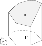
Figure 2. Tetrahedron, pyramide, and prizm

At vertexes A, B, and C, we define three constant vectors

$$\widehat{\boldsymbol{\tau}}_{A}=\frac{{{\boldsymbol{\eta}}}}{|{\boldsymbol{\eta}}|\sin\alpha},\quad\widehat{\boldsymbol{\tau}}_{A}=\frac{{{\boldsymbol{\zeta}}}}{|{\boldsymbol{\zeta}}|\sin\beta},\quad{\rm and}\quad\widehat{\boldsymbol{\tau}}_{A}=\frac{{{\boldsymbol{\sigma}}}}{|{\boldsymbol{\sigma}}|\sin\gamma}.$$

The vector field ${\boldsymbol{\tau}}(x_{1},x_{2},x_{3})$ is the affine field in $\Omega$ with zero value at the vertex O. We compute

$$\int\limits_{\Omega}|\tau|^{2}\,dx=\int\limits^{h}_{0}\left(\;\int\limits_{\omega(x_{3})}|\tau(x_{1},x_{2},x_{3})|^{2}dx_{1}dx_{2}\right)dx_{3}.$$

Notice that the cross section $\omega(x_{3})$ associated with the height $x_{3}$ has the measure $|\omega(x_{3})|=\left(1-\frac{x_{3}}{h}\right)^{2}|\Gamma|$ and at the respective point $A^{\prime}$ on $OA$ (which third coordinate is $x_{3}$) by linear proportion we have ${\boldsymbol{\tau}}_{A^{\prime}}=\left(1-\frac{x_{3}}{h}\right)\widehat{\boldsymbol{\tau}}_{A}$. Similar relations hold for the points $B^{\prime}$ and $C^{\prime}$ associated with the cross section on the height $x_{3}$. For the internal integral we apply the Gaussian quadrature for $|\tau|^{2}=\tau^{2}_{1}+\tau^{2}_{2}+\tau^{3}_{3}$ and obtain

(2.6) $$\displaystyle C^{2}_{\Gamma}\,\leq\,\frac{{\rm d}^{2}_{\Omega}}{\pi^{2}}+\frac{|{\boldsymbol{\eta}}|^{2}+|{\boldsymbol{\zeta}}|^{2}+|{\boldsymbol{\sigma}}|^{2}+{{\boldsymbol{\eta}}}\cdot{{\boldsymbol{\zeta}}}+{{\boldsymbol{\eta}}}\cdot{{\boldsymbol{\sigma}}}+{{\boldsymbol{\zeta}}}\cdot{{\boldsymbol{\sigma}}}}{90}$$

In particular, for the equilateral tetrahedron with all edges equal to $h$ we have

$${\boldsymbol{\eta}}\cdot{\boldsymbol{\zeta}}={\boldsymbol{\eta}}\cdot{\boldsymbol{\sigma}}={\boldsymbol{\zeta}}\cdot{\boldsymbol{\sigma}}=\frac{1}{2}h^{2},\quad{\rm d}_{\Omega}=h,$$

and, therefore, $C_{\Gamma}\,\leq\,h\sqrt{\frac{1}{\pi^{2}}+\frac{1}{20}}\approx 0.39h.$

For the right tetrahedron with nodes $(0,0,0)$, $(h,0,0)$, $(0,h,0)$, $(0,0,h)$ and face $\Gamma=\{x\in\overline{\Omega},\,x_{3}=0\}$, we have ${\rm d}_{\Omega}=h\sqrt{2}$, $|\eta|=h$, $|\zeta|=|\sigma|=h\sqrt{2}$, scalar products are equal to $h^{2}$ and (2.6) yields $C_{\Gamma}\,\leq\,h\sqrt{\frac{2}{\pi^{2}}+\frac{4}{45}}\approx 0.54h.$ Sharp constants $C_{\Gamma}$ for triangle and tetrahedrons has been recently evaluated in [20]. For the right tetrahedron, the constant computed in [20] numerically is $C_{\Gamma}\approx 0.3756h$.

2.4. Pyramide

We can apply (2.6) in order to evaluate $C_{\Gamma}$ for a pyramid OABCD, which can be divided into two tetrahedrons OABC and OACD (Fig. 2 middle, view from above). Assume that the triangles ABC and ACD have equal areas and $\Gamma$ is the pyramid basement ABCD. Then, we can use (2.1) with $\tau$ defined in each tetrahedron as in 2.3. We obtain

(2.7) $$C^{2}_{\Gamma}\,\leq\,\frac{{\rm d}^{2}_{\Omega}}{\pi^{2}}+\frac{2|{\boldsymbol{\eta}}|^{2}+|{\boldsymbol{\zeta}}|^{2}+2|{\boldsymbol{\sigma}}|^{2}+|{\boldsymbol{\chi}}|^{2}+2{{\boldsymbol{\eta}}}\cdot{{\boldsymbol{\sigma}}}+({{\boldsymbol{\eta}}}+{\boldsymbol{\sigma}})\cdot({{\boldsymbol{\chi}}}+{{\boldsymbol{\zeta}}})}{180}.$$

2.5. Prizmatic cells

Consider domains of the form (Fig. 2 right).

$$\Omega=\{x\in{\mathbb{R}}^{3}\,\mid\,(x_{1},x_{2})\in\Gamma,\quad 0\leq\,x_{3}\,\leq H(x_{1},x_{2}),\quad H(x_{1},x_{2})\geq H_{min}\}.$$

By the same method as in 2.1 we find that

(2.8) $$C^{2}_{\Gamma}\,\leq\,\overline{C}^{2}_{\Gamma}:=C^{2}_{\rm P}+\left(\frac{\left\{\!\!\left|\,H\,\right|\!\!\right\}_{\Gamma}}{\sqrt{3}}+C_{\rm P}\,\kappa\right)^{2}.$$

where $\kappa=\left(\frac{\left\{\!\!\left|\,H\,\right|\!\!\right\}_{\Gamma}}{H_{min}}-1\right)^{1/2}$ characterises variations of the mean height.

In particular, if $H=const$ (so that $\kappa=0$) and $\Gamma$ is a convex domain in ${\mathbb{R}}^{d-1}$, then

(2.9) $$C^{2}_{\Gamma}\,\leq\,\frac{{\rm d}^{2}_{\Gamma}+H^{2}}{\pi^{2}}+\frac{H^{2}}{3}=\frac{1}{\pi^{2}}\left({\rm d}^{2}_{\Gamma}+\left(1+\frac{\pi^{2}}{3}\right)H^{2}\right).$$

For a parallelepiped with $\Gamma=(0,a)\times(0,b)$, we know that the exact value of $C_{\Gamma}$ is $\frac{1}{\pi}\max\{2H,a,b\}$. In this case ${\rm d}^{2}_{\Gamma}=a^{2}+b^{2}$ and we can compare it with the upper bound that follows from (2.8):

(2.10) $$\frac{\overline{C}_{\Gamma}}{C_{\Gamma}}=\frac{\sqrt{a^{2}+b^{2}+4.29H^{2}}}{\max\{2H,a,b\}}\geq 1.$$

For the cases where one dimension of $\Omega$ dominates, $\overline{C}_{\Gamma}$ is a good approximation of $C^{2}_{\Gamma}$. If $a=b=H$ (cube), then we have $\frac{\overline{C}_{\Gamma}}{C_{\Gamma}}=\frac{\sqrt{6.29}}{2}\approx 1.25$. The largest ratio is for $a=b=2H$ ( $\approx 1.75$).

3. Boundary Poincaré inequalities for vector valued functions

Estimates (1.10) and (1.11) yield analogous estimates for vector valued functions in $H^{1}(\Omega,\mathbb{R}^{d})$. Let $\Omega\in\mathbb{R}^{d}$ ( $d\geq 1$) be a connected domain with $N$ plane faces $\Gamma_{i}\in{\mathbb{R}}^{d-1}$. Assume that we have $d$ unit vectors ${\bf n}^{(k)}$, (associated with some faces) that form a linearly independent system in $\mathbb{R}^{d}$, i.e.,

(3.1) $${\det{\bf N}\not=0},\qquad{\bf N}:=\left\{n^{(i)}_{j}\right\}\in{\mathbb{M}}^{d\times d},\quad i,j=1,2,...,d,$$

where $n^{(i)}_{j}={\bf n}^{(i)}\cdot{\bf e}_{j}$ and ${\bf e}_{i}$ denote the Cartesian orts. Then, ${\bf v}\in H^{1}(\Omega,\mathbb{R}^{d})$ satisfies a Poincaré type estimate provided that it satisfies zero mean conditions (3.2).

Theorem 3.1.

If (3.1) holds and

(3.2) $$\left\{\!\!\left|\,{\bf v}\cdot{\bf n}^{(i)}\,\right|\!\!\right\}_{\Gamma_{i}}=0\quad i=1,2,...,d,$$

then

(3.3) $$\|{\bf v}\|_{\Omega}\,\leq\,{\mathds{C}}(\Omega,\Gamma_{1},...,\Gamma_{d})\|\nabla{\bf v}\|_{\Omega},$$

where ${\mathds{C}}>0$ depends only on geometrical properties of the cell.

Proof.

Assume the opposite. Then, there exists a sequence $\{{\bf v}_{k}\}$ such that $\left\{\!\!\left|\,{\bf v}_{k}\cdot{\bf n}^{(i)}\,\right|\!\!\right\}_{\Gamma_{i}}=0$ and

(3.4) $$\|{\bf v}_{k}\|\geq\,k\,\|\nabla{\bf v}_{k}\|.$$

Without a loss of generality we can operate with a sequence of normalised functions, so that

(3.5) $$\|{\bf v}_{k}\|=1.$$

Hence,

(3.6) $$\|\nabla{\bf v}_{k}\|\leq\,\frac{1}{k}\,\rightarrow\,0\;{\rm as}\;k\rightarrow+\infty.$$

We conclude that there exists a subsequence (for simplicity we omit additional subindexes and keep the notation $\{{\bf v}_{k}\}$) such that

(3.7) $${\bf v}_{k}\,\rightharpoonup\,{\bf w}\; {\rm in}\;H^{1}(\Omega,\mathbb{R}^{d}),$$

(3.8) $${\bf v}_{k}\,\rightarrow\,{\bf w}\; {\rm in}\;L^{2}(\Omega,\mathbb{R}^{d}).$$

In view of (3.7),

$$0=\lim\inf_{k\rightarrow+\infty}\|\nabla{\bf v}_{k}\|\,\geq\,\|\nabla{\bf w}\|,$$

we see that ${\bf w}\in P^{0}(\Omega,\mathbb{R}^{d})$. For any face $\Gamma_{i}$ we have (in view of the trace theorem)

(3.9) $$\|{\bf v}_{k}-{\bf w}\|_{2,\Gamma_{i}}\leq C\left(\|{\bf v}_{k}-{\bf w}\|_{2,\Omega}+\|\nabla{\bf v}_{k}\|_{2,\Omega}\right).$$

We recall (3.6) and (3.8) and conclude that the traces of ${\bf v}_{k}$ on ${\Gamma_{i}}$ converge to the trace of ${\bf w}$. Since ${\bf v}_{k}\cdot{\bf n}^{(i)}$ have zero means,

(3.10) $${\bf w}\cdot{\bf n}_{i}|\Gamma_{i}|=\int\limits_{\Gamma_{i}}{\bf w}\cdot{\bf n}_{i}\,d\Gamma=0$$

and ${\bf w}$ is orthogonal to $d$ linearly independent vectors, i.e., ${\bf w}=0$. On the other hand, $\|{\bf w}\|=1$. We obtain a contradiction, which shows that the assumption is not true. ∎

We notice that conditions of the Theorem are very flexible with respect to choosing $\Gamma_{i}$ and vectors ${\bf n}^{(i)}$ entering the integral type conditions (3.2). Probably the most interesting case is where ${\bf n}^{(i)}$ are defined as unit outward normals to faces $\Gamma_{s}$. If $d=2$, then we can also define ${\bf n}^{(i)}$ as unit tangential vectors. Moreover, in the proof it is not essential that ${\bf n}^{(i)}$ is strictly related to one face $\Gamma_{i}$ (only the condition (3.1) is essential). For example, if $d=3$ then we can define two vectors as two mutually orthogonal tangential vectors of one face and the third one as a normal vector to another face. Theorem holds for this case as well. Henceforth, for the sake of definiteness we assume that ${\bf n}^{(i)}$ are normal vectors or mean normal vectors (for curvilinear faces) associated with faces $\Gamma_{i}$, $i=1,2,...,d$. Possible modifications of the results to other cases are rather obvious.

3.1. Value of the constant for $d=2$

Estimates of the constant ${\mathds{C}}(\Omega,\Gamma_{1},...,\Gamma_{d})$ follow from (1.10) and depend on the constants $C_{\Gamma_{i}}(\Omega)$. Now, our goal is to deduce explicit and easily computable bounds of ${\mathds{C}}(\Omega,\Gamma_{1},...,\Gamma_{d})$.

First, we consider a special, but important case where $\Omega$ is a polygonal domain in ${\mathbb{R}}^{2}$. Let $\Gamma_{1}$ and $\Gamma_{2}$ be two faces selected for the interpolation of ${\bf v}$. The respective normals ${\bf n}^{(1)}=(n^{(1)}_{1},n^{(1)}_{2})$ and ${\bf n}^{(2)}=(n^{(2)}_{1},n^{(2)}_{2})$ must satisfy the condition (3.1), which means that

(3.11) $$\angle({\bf n}^{(1)},{\bf n}^{(2)})=\beta\in(0,\pi).$$

Let the conditions (3.2) hold. Then

(3.12) $$\|n^{(1)}_{1}v_{1}+n^{(1)}_{2}v_{2}\|^{2}\leq C^{2}_{\Gamma_{1}}(\Omega)\|n^{(1)}_{1}\nabla v_{1}+n^{(1)}_{2}\nabla v_{2}\|^{2},$$

(3.13) $$\|n^{(2)}_{1}v_{1}+n^{(2)}_{2}v_{2}\|^{2}\leq C^{2}_{\Gamma_{2}}(\Omega)\|n^{(2)}_{1}\nabla v_{1}+n^{(2)}_{2}\nabla v_{2}\|^{2}.$$

Introduce the matrix

$${{\bf T}}:={\bf n}^{(1)}\otimes{\bf n}^{(1)}+\!{\bf n}^{(2)}\otimes{\bf n}^{(2)}\!=\!\left(\begin{array}[]{cc}(n^{(1)}_{1})^{2}+(n^{(2)}_{1})^{2}&\;n^{(1)}_{1}n^{(1)}_{2}+n^{(2)}_{1}n^{(2)}_{2}\\ n^{(1)}_{1}n^{(1)}_{2}+n^{(2)}_{1}n^{(2)}_{2}&(n^{(1)}_{2})^{2}+(n^{(2)}_{2})^{2}\end{array}\right).$$

Here and later on $\otimes$ denotes the diadic product of vectors. Summation of (3.12) and (3.13) yields

(3.15) $$\int\limits_{\Omega}{{\bf T}}{\bf v}\cdot{\bf v}dx_{1}dx_{2}\\ \leq C^{2}\int\limits_{\Omega}(T_{11}|\nabla v_{1}|^{2}+2T_{12}\nabla v_{1}\cdot\nabla v_{2}+T_{22}|\nabla v_{2}|^{2})dx_{1}dx_{2},$$

where

$$C=\max\{C_{\Gamma_{1}}(\Omega);C_{\Gamma_{2}}(\Omega)\}.$$

It is easy to see that ${\bf T}$ is a positive definite matrix. Indeed,

$$\det({\bf T}-\lambda{\bf E})\\ =((n^{(1)}_{1})^{2}+(n^{(2)}_{1})^{2}-\lambda)((n^{(1)}_{2})^{2}+(n^{(2)}_{2})^{2}-\lambda)-\bigl{(}n^{(1)}_{1}n^{(1)}_{2}+n^{(2)}_{1}n^{(2)}_{2}\bigr{)}^{2}\\ =\lambda^{2}-2\lambda+\bigl{(}n^{(1)}_{1}n^{(2)}_{2}-n^{(2)}_{1}n^{(1)}_{2}\bigr{)}^{2}=\lambda^{2}-2\lambda+\left(\det{{\bf N}}\right)^{2},$$

where

$${{\bf N}}:=\left(\begin{array}[]{c}{\bf n}^{(1)}\\ {\bf n}^{(2)}\end{array}\right).$$

Hence for any vector ${\bf b}$, we have $\lambda_{1}|{{\bf b}}|^{2}\leq\,{{\bf T}{\bf b}\cdot{\bf b}}\,\leq\,\lambda_{2}|{{\bf b}}|^{2},$ and

(3.17) $$\lambda_{1,2}=1\mp\sqrt{1-\left(\det{{\bf N}}\right)^{2}}.$$

If ${\bf n}^{(1)}$ and ${\bf n}^{(1)}$ are orthogonal, then $\det{{\bf N}}=1$ and the unique eigenvalue of ${\bf N}$ is $\lambda=1$. In this case, the left hand side of (3.15) coincides with $\|{\bf v}\|^{2}$. In all other cases $\det{{\bf N}}<1$ and $\lambda_{1}<\lambda_{2}$.

We can always select the coordinate system such that

$$n^{(1)}_{1}=1,\;n^{(1)}_{2}=0,\;n^{(2)}_{1}=-\cos\beta,\;n^{(2)}_{2}=\sin\beta.$$

Then,

$$T_{11}=1+\cos^{2}\beta,\;T_{22}=1-\cos^{2}\beta,\;T_{12}=-\sin\beta\cos\beta,$$

and the matrix is

$${{\bf N}}:=\left(\begin{array}[]{cc}1&\;0\\ -\cos\beta&\;\sin\beta\end{array}\right).$$

We see that $\det{{\bf N}}=\sin\beta$, and $\lambda_{1}=1-\left|\cos\beta\right|$.

Consider the right hand side of (3.15). It is bounded from above by the quantity

$$I({\bf v}):=C^{2}\int\limits_{\Omega}\left((T_{11}+\gamma|T_{12}|)|\nabla v_{1}|^{2}+(T_{22}+\gamma^{-1}|T_{12}|)|\nabla v_{2}|^{2}\right)dx,$$

where $\gamma$ is any positive number. We define $\gamma$ by means of the relation $T_{11}-T_{22}=(\gamma^{-1}-\gamma)|T_{12}|$, which yields $\gamma=\frac{1-|\cos\beta|}{\sin\beta}$. Then,

(3.19) $$I({\bf v})\,\leq\,(1+|\cos\beta|)\|\nabla{\bf v}\|^{2}.$$

From (3.15) and (3.19), we find that

(3.23)

This is the Poincaré type inequality for the vector valued function ${\bf v}$ with zero mean normal traces on $\Gamma_{1}$ and $\Gamma_{2}$. It is worth noting that for small $\beta$ (and for $\beta$ close to $\pi$) the constant blows up. Therefore, interpolation operators (considered in Sect. 4) should avoid such situations.

3.2. Value of the constant for $d\geq 3$

Now we are concerned with the general case and deduce the estimate valid for any dimension $d$.

In view of (3.2) we have

(3.24) $$\sum\limits^{d}_{k=1}\|{\bf n}^{(k)}\cdot{\bf v}\|^{2}_{2,\Omega}\,\leq\,C^{2}\,\sum\limits^{d}_{k=1}\int\limits_{\Omega}\Bigl{(}\sum\limits^{d}_{i=1}n^{(k)}_{i}\nabla v_{i}\Bigr{)}^{2}\,d{\bf x},2(\Omega,\Gamma_{3})\|n^{(3)}_{1}\nabla v_{1}+n^{(3)}_{2}\nabla v_{2}+n^{(3)}_{3}\nabla v_{3}\|^{2}$$

where

$$C=\max\limits_{k=1,2,...,d}\;\left\{C_{\Gamma_{k}}(\Omega)\right\}.$$

In view of the relation

$$({\bf n}^{(k)}\otimes{\bf n}^{(k)}){\bf v}\cdot{\bf v}=({\bf n}^{(k)}({\bf n}^{(k)}\cdot{\bf v}))\cdot{\bf v}=({\bf n}^{(k)}\cdot{\bf v})^{2},$$

the left hand side of (3.24) is $\int\limits_{\Omega}{{\bf T}}{\bf v}\cdot{\bf v},$ where

(3.25) $${\bf T}:=\sum\limits^{d}_{k=1}{\bf n}^{(k)}\otimes{\bf n}^{(k)}.\qquad$$

If ${\bf n}^{(k)}$ form a linearly independent system, then ${\bf T}$ is a positive definite matrix. Indeed, ${\bf T}{\bf b}\cdot{\bf b}=\sum\limits^{d}_{k=1}({\bf n}^{(k)}\cdot{\bf b})^{2}$. Hence, ${\bf T}{\bf b}\cdot{\bf b}=0$ if and only if ${\bf b}$ has zero projections to $d$ linearly independent vectors ${\bf n}^{(k)}$, i.e., ${\bf T}{\bf b}\cdot{\bf b}=0$ if and only if ${{\bf b}}=0$. Therefore,

(3.26) $$\lambda_{1}\,\|{\bf v}\|^{2}\,\leq\,\int\limits_{\Omega}{{\bf T}{\bf v}\cdot{\bf v}}\,d{\bf x},$$

where $\lambda_{1}>0$ is the minimal eigenvalue of ${\bf T}$.

Consider the right hand side of (3.24). We have

$$\int\limits_{\Omega}\Bigl{(}\sum\limits^{d}_{i=1}n^{(k)}_{i}\nabla v_{i}\Bigr{)}^{2}d{\bf x}=\int\limits_{\Omega}\sum\limits^{d}_{i,j=1}n^{(k)}_{i}n^{(k)}_{j}\nabla v_{i}\cdot\nabla v_{j}d{\bf x}\\ =\sum\limits^{d}_{i,j=1}n^{(k)}_{i}n^{(k)}_{j}\int\limits_{\Omega}\nabla v_{i}\cdot\nabla v_{j}d{\bf x}={\bf n}^{(k)}\otimes{\bf n}^{(k)}:{\bf G},$$

where

$${\bf G}({\bf v}):=\{G_{ij}\},\quad G_{ij}({\bf v})=\int\limits_{\Omega}\nabla v_{i}\cdot\nabla v_{j}d{\bf x}.$$

Hence,

(3.27) $$\sum\limits^{d}_{k=1}\int\limits_{\Omega}\Bigl{(}\sum\limits^{d}_{i=1}n^{(k)}_{i}\nabla v_{i}\Bigr{)}^{2}\,d{\bf x}={\bf T}:{\bf G}({\bf v})\,\leq\,|{\bf T}|\,|{\bf G}({\bf v})|.$$

Now (3.24), (3.25), (3.26), and (3.27) yield the estimate

$$\|{\bf v}\|^{2}\,\leq\,C^{2}\frac{1}{\lambda_{1}}|{\bf T}|\,|{\bf G}({\bf v})|\leq\,C^{2}\frac{d}{\lambda_{1}}\,|{\bf G}({\bf v})|.$$

Since $|{\bf G}({\bf v})|\leq\,\|\nabla{\bf v}\|^{2}$, for any ${\bf v}\in H^{1}(\Omega,\mathbb{R}^{d})$ satisfying (3.2) we have

(3.31)

In other words, the constant in (3.31) can be defined as follows:

(3.32) $$\mathds{C}(\Omega,\Gamma_{1},\Gamma_{2},...,\Gamma_{d})\,=\,\max\limits_{k=1,2,...,d}\{C_{\Gamma_{k}}(\Omega)\}\;\sqrt{\frac{d}{\lambda_{1}}},$$

where $\lambda_{1}$ is the minimal eigenvalue of ${\bf T}$.

For $d=2$ this estimate exposes a slightly worse constant than (3.23) with the factor $\sqrt{\frac{2}{1-|\cos\beta|}}$ instead of $\sqrt{\frac{1+|\cos\beta|}{1-|\cos\beta|}}$.

4. Interpolation of functions

The classical Poincaré inequality (1.1) yields a simple interpolation operator ${\mathbb{I}}_{\Omega}:H^{1}(\Omega)\,\rightarrow\,P^{0}(\Omega)$ defined by the relation ${\mathbb{I}}_{\Omega}w:=\left\{\!\!\left|\,w\,\right|\!\!\right\}_{\Omega}$. In view of (1.1), we know that

(4.1) $$\|w-{\mathbb{I}}_{\Omega}w\|_{2,\Omega}\,\leq\,C_{\rm P}(\Omega)\|\nabla w\|_{2,\Omega},$$

which means that the interpolation operator is stable and $C_{\rm P}(\Omega)$ is the respective constant.

Above discussed estimates for functions with zero mean traces yield somewhat different interpolation operators for scalar and vector valued functions. For a scalar valued function $w\in H^{1}(\Omega)$, we set ${\mathds{I}}_{\Gamma}(w):=\left\{\!\!\left|\,w\,\right|\!\!\right\}_{\Gamma}$, i.e., the interpolation operator uses mean values of $w$ a $d-1$ – dimensional set $\Gamma$. Since $\left\{\!\!\left|\,w-{\mathds{I}}_{\Gamma}w\,\right|\!\!\right\}_{\Gamma}=0$, we use (1.10) and obtain the interpolation estimate

(4.2) $$\|w-{\mathbb{I}}_{\Gamma}w\|_{2,\Omega}\,\leq\,C_{\Gamma}(\Omega)\|\nabla w\|_{2,\Omega},$$

where the constant $C_{\Gamma}$ appears as the interpolation constant. Analogously, (1.11) yields an interpolation estimate for the boundary trace

(4.3) $$\|w-{\mathbb{I}}_{\Gamma}w\|_{2,\Gamma}\,\leq\,C^{\rm Tr}_{\Gamma}\|\nabla w\|_{2,\Omega}.$$

Applying these estimates to cells of meshes we obtain analogous interpolation estimates for mesh interpolation of scalar functions with explicit constants depending on character diameter of cells.

For the interpolation of vector valued functions we use (3.31) and generalise this idea.

4.1. Cells with plane faces

Define the operator

$${\mathds{I}}_{\Gamma_{1},\Gamma_{2},...,\Gamma_{d}}:H^{1}(\Omega,\mathbb{R}^{d})\,\rightarrow\,P^{0}(\Omega,\mathbb{R}^{d})$$

that performs zero order interpolation of a vector valued function ${\bf v}$ using mean values of normal components on the faces $\Gamma_{i}$, $i=1,2,...,d$. In this case, we set

(4.4) $$\int\limits_{\Gamma_{i}}\left({\mathds{I}}_{\Gamma_{1},\Gamma_{2},...,\Gamma_{d}}{\bf v}\right)\cdot{\bf n}^{(i)}\,d\Gamma=\int\limits_{\Gamma_{i}}{\bf v}\cdot{\bf n}^{(i)}\,d\Gamma\qquad i=1,2,...,d.$$

This condition means that the intrpolant must preserve integral values of normal flux through $d$ selected faces. In general we may define several different operators associated with different collections of faces. However, once the set of $\Gamma_{1},\Gamma_{2},...,\Gamma_{d}$ satisfying (3.1) has been defined, the operator ${\mathds{I}}_{\Gamma_{1},\Gamma_{2},...,\Gamma_{d}}$ uniquely defines the vector ${\mathds{I}}_{\Gamma_{1},\Gamma_{2},...,\Gamma_{d}}\,{\bf v}$. In view of (4.4) and the identity

$$\left({\mathds{I}}_{\Gamma_{1},\Gamma_{2},...,\Gamma_{d}}{\bf v}\right)\cdot{\bf n}^{(i)}=({\mathds{I}}_{\Gamma_{1},\Gamma_{2},...,\Gamma_{d}}{\bf v})_{j}{\bf e}_{j}\cdot{\bf n}^{(i)},$$

we conclude that the components of the interpolant are uniquely defined by the system

(4.5) $$\sum\limits^{d}_{j=1}n^{(i)}_{j}({\mathds{I}}_{\Gamma_{1},\Gamma_{2},...,\Gamma_{d}}\,{\bf v})_{j}=\frac{1}{|\Gamma_{i}|}\int\limits_{\Gamma_{i}}{\bf v}\cdot{\bf n}^{(i)}\,d\Gamma\quad i=1,2,...,d.$$

Define ${\bf w}:={\bf v}-{\mathds{I}}_{\Gamma_{1},\Gamma_{2},...,\Gamma_{s}}{\bf v}$. From (4.4), it follows that

$$\left\{\!\!\left|\,{\bf w}\cdot{\bf n}^{(i)}\,\right|\!\!\right\}_{\Gamma_{i}}=0\qquad i=1,2,...,d.$$

Therefore, we can apply Theorem 3.1 to ${\bf w}$ and find that

(4.6) $$\|{\bf w}\|_{\Omega}\,\leq\,{\mathds{C}}(\Omega,\Gamma_{1},...,\Gamma_{d})\|\nabla{\bf w}\|_{\Omega}.$$

Since $\nabla{\bf w}=\nabla\bf v$, (4.6) yields the estimate

(4.10)

where ${\mathds{C}}(\Omega,\Gamma_{1},...,\Gamma_{d})$ depends on the constants $C_{\Gamma_{i}}$ (see section 3.2).

4.2. Cells with curvilinear faces

Let $\Omega$ be a Lipschitz domain with a piecewise smooth boundary consisting of smooth parts $\Gamma_{1}$, $\Gamma_{2}$,…,$\Gamma_{N}$ (see Fig. 3). In order to avoid complicated topological structures (which may lead to difficulties with definitions of ”mean normals”), we assume that all the faces are such that normal vectors can be defined at almost all points and impose an additional condition

$${\bf n}_{i}(x^{(1)})\cdot{\bf n}_{i}(x^{(2)})>0\qquad\forall x^{(1)},x^{(2)}\in\Gamma_{i},\quad i=1,2,...,d.$$

Then, we can define the mean normal vector associated with $\Gamma_{i}$:

$$\widehat{\bf n}{(i)}:=\left\{\frac{1}{|\Gamma_{i}|}\int\limits_{\Gamma_{i}}n^{(i)}_{1}\,d\Gamma,\frac{1}{|\Gamma_{i}|}\int\limits_{\Gamma_{i}}n^{(i)}_{2}\,d\Gamma,...,\frac{1}{|\Gamma_{i}|}\int\limits_{\Gamma_{i}}n^{(i)}_{d}\,d\Gamma\right\}.$$

    

Figure 3. Cells with curvilinear faces in 2D and 3D

It is not difficult to verify that Theorem 3.1 holds if ${\bf N}$ is replaced by $\widehat{\bf N}$ formed by mean normal vectors, i.e.,

(4.11) $$\;\det{\widehat{\bf N}}\not=0,\qquad{\rm where}\qquad\widehat{n}^{(i)}_{j}:=\widehat{\bf n}^{(i)}\cdot{\bf e}_{j},$$

and (3.2) is replaced by the condition

(4.12) $$\left\{\!\!\left|\,{\bf v}\cdot\widehat{\bf n}^{(i)}\,\right|\!\!\right\}_{\Gamma_{i}}=0\quad i=1,2,...,d.$$

In other words, for cells with curvilinear faces the necessary interpolation condition reads as follows: mean values of normal vectors averaged on faces must form a linearly independent system satisfying (4.11).

The operator ${\mathds{I}}_{\Gamma_{1},\Gamma_{2},...,\Gamma_{d}}\,{\bf v}$ is defined by modifying the condition (4.4). Since

$$\int\limits_{\Gamma_{i}}{\mathds{I}}_{\Gamma_{1},\Gamma_{2},...,\Gamma_{d}}{\bf v}\cdot{\bf n}^{(i)}\,d\Gamma={\mathds{I}}_{\Gamma_{1},\Gamma_{2},...,\Gamma_{d}}{\bf v}\cdot\widehat{\bf n}^{(i)}\,\bigl{|}\Gamma_{i}\bigr{|},$$

the interpolant ${\mathds{I}}_{\Gamma_{1},\Gamma_{2},...,\Gamma_{d}}\,{\bf v}$ is defined by the system

(4.13) $$\sum\limits^{d}_{j=1}\widehat{n}^{(i)}_{j}({\mathds{I}}_{\Gamma_{1},\Gamma_{2},...,\Gamma_{d}}\,{\bf v})_{j}=\frac{1}{|\Gamma_{i}|}\int\limits_{\Gamma_{i}}{\bf v}\cdot{\bf n}^{(i)}\,d\Gamma\quad i=1,2,...,d.$$

By repeating the same arguments, we obtain the estimate (4.10) for the interpolant ${\mathds{I}}_{\Gamma_{1},\Gamma_{2},...,\Gamma_{d}}{\bf v}$.

4.3. Comparison of interpolation constants for ${\mathds{I}}_{\Omega}$ and ${\mathds{I}}_{\Gamma}$

4.3.1. Triangles

First, we compare five different interpolation operators for the right triangle with equal legs (see Fig. 1). For the interpolation operator ${\mathds{I}}_{\Omega}$ (Fig. 1a) we have (1.9), where (1.6) yields the upper bound of the respective interpolation constant $C_{\rm P}(\Omega)\,\leq\,\sqrt{2}\frac{h}{\pi}\approx 0.4502h$.

  

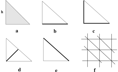
Figure 4. Triangular cells

Four different operators ${\mathds{I}}_{\Gamma}$ are generated by setting zero mean values on one leg (b), two legs (c), median (d), and hypothenuse (e)

$$\|w-{\mathbb{I}}_{\Gamma}(w)\|_{2,\Omega}\,\leq\;C_{\Gamma}(\Omega)h\|\nabla w\|_{2,\Omega}.$$

The respective constants follow from Tab. 1. For (b), $C_{\Gamma}(\Omega)=\frac{h}{\zeta}\approx 0.4929h$, for (c) $C_{\Gamma}(\Omega)=\frac{h}{\pi}\approx 0.3183h$, for (d) and (e) $C_{\Gamma}(\Omega)=\frac{h}{\zeta\sqrt{2}}\approx 0.3485h$.

We can use these data and compare the efficiency of ${\mathds{I}}_{\Gamma}$ and ${\mathds{I}}_{\Omega}$ for uniform meshes which cells are right equilateral triangles (Fig. 1 f). For a mesh with $2nm$ cells, the operator ${\mathds{I}}_{\Omega}$ uses $2nm$ parameters (mean values on triangles) and provides interpolation with the constant $C_{\rm P}$. The operator ${\mathds{I}}_{\Gamma}$ using mean values on diagonals (see (e)) has almost the same constant but needs only $mn$ parameters.

4.3.2. Squares

Similar results hold for square cells. For the interpolation operator ${\mathds{I}}_{\Omega}$ (Fig. 2a) we have the exact constant $C_{\rm P}=\frac{\pi}{h}$. The constants for ${\mathds{I}}_{\Gamma}$ are as follows. For (b), $C_{\Gamma}=\frac{h}{\pi}$, for (c) and (d) $C_{\Gamma}=\frac{2h}{\pi}$, and for (e) $C_{\Gamma}=\frac{h}{2.869}$. We see that for a uniform mesh with square cells ${\mathds{I}}_{\Gamma}$ and ${\mathds{I}}_{\Omega}$ have the same efficiency if $\Gamma$ is selected as on (d) or (e).

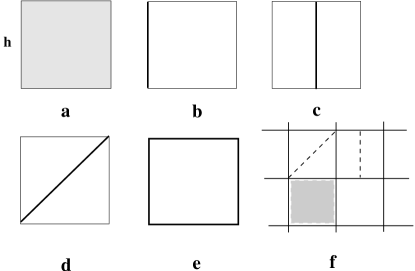
Figure 5. Square cells

4.4. Interpolation on macrocells

Advanced numerical approximations often operate with macrocells. Let $\Omega$ be a macrocell consisting of $N$ simple subdomains $\omega_{i}$ (e.g., simplexes). Let the boundary $\Gamma$ consist of faces $\Gamma_{i}$ (each $\Gamma_{i}$ is a part of some subdomain boundary $\partial\omega_{i}$). For $w\in H^{1}(\Omega)$ we define ${\mathds{I}}_{\Gamma}w$ as a piecewise constant function that satisfies the conditions

(4.14) $$\left\{\!\!\left|\,w-{\mathds{I}}_{\Gamma}w\,\right|\!\!\right\}_{\Gamma_{i}}=0\qquad i=1,2,...,N.$$

Then, we can apply interpolation operators ${\mathds{I}}_{\gamma_{i}}$ to any subdomain $\omega_{i}$ and find that for the whole cell

(4.15) $$\|w-{\mathds{I}}_{\Gamma}w\|^{2}_{2,\Omega}=\sum\limits^{N}_{i=1}\|w-{\mathds{I}}_{\Gamma}w\|^{2}_{2,\omega_{i}}\\ \leq\sum\limits^{N}_{i=1}C^{2}_{\gamma_{i}}\|\nabla w\|^{2}_{2,\omega_{i}}\,\leq\,C^{2}_{\Gamma}\|\nabla w\|^{2}_{2,\Omega},$$

where $C_{\Gamma}=\max\limits_{i}\{C_{\Gamma_{i}}\}$.

Estimates for vector valued functions are derived quite similarly. For example, let $d=2$ and $\Omega$ be a polygonal domain with $N$ faces. If $N$ is an odd number, then we form out of $\Gamma_{i}$ a set of $K$ pairs $\{\Gamma^{(l)}_{1},\Gamma^{(l)}_{2}\}$, $l=1,2,...,K$ such that the respective subdomains cover $\Omega$ and for each pair ${\bf n}^{(l)}_{1}$ and ${\bf n}^{(l)}_{2}$ satisfy (3.1). Then, the interpolant ${\mathds{I}}_{\Gamma}{\bf v}$ can be defined as a piece vise constant field in each pair of subdomains $\omega^{(l)}_{1}\cup\omega^{(l)}_{2}$ that satisfies

(4.16) $$\left\{\!\!\left|\,({\bf v}-{\mathds{I}}_{\Gamma}{\bf v})\cdot{\bf n}_{i}\,\right|\!\!\right\}_{\Gamma_{i}}=0\qquad i=1,2,...,N.$$

Analogously to (4.15, we obtain

(4.17) $$\|{\bf v}-{\mathds{I}}_{\Gamma}{\bf v}\|_{2,\Omega}\,\leq\,{\mathds{C}}\|\nabla{\bf v}\|_{2,\Omega}\qquad{\bf v}\in H^{1}(\Omega,{\mathbb{R}}^{2}),$$

where ${\mathds{C}}=\max\limits_{l=1,2,...,K}{\mathds{C}}_{\Gamma^{(l)}_{1},\Gamma^{(l)}_{2}}(\omega^{(l)}_{1}\cup\omega^{(l)}_{2})$.

4.5. Interpolation on meshes

Finally, we shortly discuss applications to mesh interpolation. It is clear that analogous operators ${\mathds{I}}_{\Gamma}$ can be constructed for scalar and vector valued functions defined in a bounded Lipschitz domain $\Omega$, which is covered by a mesh ${\mathcal{T}}_{h}$ with sells $\Omega_{i}$, $i=1,2,...,M_{h}$.

Let $\Omega_{i}$ be Lipschitz domains such that $\Omega_{i}\cup\Omega_{j}=\emptyset$ if $i\not=j$ and

(4.18) $$\overline{\Omega}=\bigcup^{M_{h}}_{i=1}\overline{\Omega}_{i}.$$

We assume that $c_{1}h\,\leq{\rm diam}\Omega_{i}\leq\,c_{2}h$ for all $i=1,2,...M_{h}$, where $c_{2}\geq c_{1}>0$ and $h$ is a small parameter. The intersection of $\overline{\Omega}_{i}$ and $\overline{\Omega}_{j}$ is either empty or a face $\Gamma_{ij}$ (which is a Lipschitz domain in ${\mathbb{R}}^{d-1}$). By ${\mathcal{E}}_{h}$ we denote the collection of all faces in ${\mathcal{T}}_{h}$.

It is easy to see that a function $w\in H^{1}({\mathcal{D}})$ can be interpolated by a piece vise constant function on cells of ${\mathcal{T}}_{h}$ if we set

(4.19) $${\mathds{I}}_{{\mathcal{T}}_{h}}(w)(x)={\mathds{I}}_{\Gamma_{i}}w(x)=\left\{\!\!\left|\,w\,\right|\!\!\right\}_{\Gamma_{i}}\qquad{\rm if}\quad x\in\Omega_{i}.$$

Here $\Gamma_{i}$ is a face of $\Omega_{i}$ selected for the local interpolation operator. Then,

(4.20) $$\|w-{\mathds{I}}_{{\mathcal{T}}_{h}}(w)\|_{2,\Omega}\;\leq\;C({\mathcal{T}}_{h})\,\|\nabla w\|_{2,\Omega},$$

where $C({\mathcal{T}}_{h})$ is the maximal constant in inequalities (1.10) associated with $\Omega_{i}$, $i=1,2,...,M_{h}$. We note that the amount of parameters used in such type interpolation is essentially smaller than the amount of faces in ${\mathcal{T}}_{h}$.

If ${\mathds{I}}_{{\mathcal{T}}_{h}}$ is constructed by means of averaging on each face $\Gamma_{ij}$ then (4.20) holds with a better constant and the interpolant ${\mathds{I}}_{{\mathcal{T}}_{h}}w$ possesses an important property: it preserves mean values of $w$.

Similar consideration is valid for vector valued functions. If we define the interpolation operator ${\mathds{I}}_{{\mathcal{T}}_{h}}({\bf v})(x)$ on ${\mathcal{T}}_{h}$ by the conditions

(4.21) $${\mathds{I}}_{{\mathcal{T}}_{h}}{\bf v}\cdot{\bf n}_{ij}=\left\{\!\!\left|\,{\bf v}\cdot{\bf n}_{{ij}}\,\right|\!\!\right\}_{\Gamma_{ij}}\qquad\forall\;\Gamma_{ij}\in{\mathcal{E}}_{h},$$

then

(4.22) $$\|{\bf v}-{\mathds{I}}_{{\mathcal{T}}_{h}}{\bf v}\|_{2,\Omega}\;\leq\;{\mathds{C}}({\mathcal{T}}_{h})\,\|\nabla{\bf v}\|_{2,\Omega},$$

where ${\mathds{C}}({\mathcal{T}}_{h})$ is the maximal constant in inequalities (4.17) used for $\Omega_{i}$, $i=1,2,...,N({\mathcal{T}}_{h})$. The interpolant ${\mathds{I}}_{{\mathcal{T}}_{h}}{\bf v}$ possesses an important property: it preserves mean values of ${\bf v}\cdot{\bf n}_{ij}$ on all the faces of ${\mathcal{T}}_{h}$.

References

- [1] D. Arnold, D. Boffi and R. Falk. Approximation by quadrilateral finite elements Math. Comp. 71 (2002), 909-922.
- [2] D. Arnold, D. Boffi and R. Falk. Quadrilateral H(div) finite elements. SIAM J. Numer. Anal. 42 (2005), no. 6, 2429–2451.
- [3] I. Babuška and A. Aziz. On the angle condition in the finite element method. SIAM J. Numer. Anal. 13 (1976), no. 2, 214–226.
- [4] A. Bermudez, P. Gamallo, M. R. Nogueiras, and R. Rodriguez. Approximation properties of lowest-order hexahedral Raviart–Thomas finite elements. Comptes Rendus Mathematique, 340 (2005), no 9, 687-692.
- [5] F. Brezzi and M. Fortin. Mixed and Hybrid Finite Element Methods. Springer, Berlin, 1991.
- [6] S. Y. Cheng. Eigenvalue comparison theorems and its geometric applications. Math. Z, 143 (1975), no. 3, 28–297.
- [7] V. Girault and P. A. Raviart. Finite element approximation of the Navier–Stokes equations. Springer-Verlag, Berlin, 1986.
- [8] D. W. Fox and J. R. Kuttler. Sloshing frequencies. Z. Angew. Math. Phys., 34 (1983), no. 5, 668–696.
- [9] V. Kozlov and N. Kuznetsov. The ice-fishing problem: the fundamental sloshing frequency versus geometry of holes. Math. Methods Appl. Sci., 27(2004), no. 3, 289–312.
- [10] V. Kozlov, N. Kuznetsov, and O. Motygin. On the two-dimensional sloshing problem. Proc. R. Soc. Lond. Ser. A Math. Phys. Eng. Sci., 460 (2004), 2587–2603.
- [11] Yu. Kuznetsov and A. Prokopenko. A new multilevel algebraic preconditioner for the diffusion equation in heterogeneous media. Numer. Linear Algebra Appl. 17 (2010), no. 5, 759–769.
- [12] Yu. Kuznetsov and S. Repin. New mixed finite element method on polygonal and polyhedral meshes, Russ. J. Numer. Anal. Math. Modelling, Vol. 18(2003), 261–278.
- [13] Yu. Kuznetsov. Mixed finite element method for diffusion equations on polygonal meshes with mixed cells. J. Numer. Math. 14 (2006), no. 4, 305 – 315.
- [14] Yu. Kuznetsov. Approximations with piece-wise constant fluxes for diffusion equations. J. Numer. Math., Vol. 19, No. 4, 309–328 (2011).
- [15] Yu. Kuznetsov Mixed FE method with piece-wise constant fluxes on polyhedral meshes. Russian J. Numer. Anal. Math. Modelling 29 (2014), no. 4, 231 – 237.
- [16] Yu. Kuznetsov. Error estimates for the RT0 and PWCF methods for the diffusion equations on triangular and tetrahedral meshes. Russian J. Numer. Anal. Math. Modelling 30 (2015), no. 2, 95 – 102.
- [17] R. S. Laugesen and B. A. Siudeja. Minimizing Neumann fundamental tones of triangles: an optimal Poincaré inequality. J Differential Equations 249 (2010), no. 1, 118–135.
- [18] O. Mali, P. Neittaanmäki and S. Repin. Accuracy Verification Methods. Theory and Algorithms, Computational Methods in Applied Sciences, 32, Springer, Dordrecht, 2014.
- [19] S. Matculevich, P. Neittaanmäki, and S. Repin. A posteriori error estimates for time-dependent reactiondiffusion problems based on the Payne–Weinberger inequality. AIMS, 35 (2015), no. 6, 2659 – 2677.
- [20] S. Matculevich and S. Repin. Sharp bounds of constants in Poincaré-type inequalities for simplicial domains. ArXiv:1504.03166v5 [math.NA], 2015 (to appear in Comput. Meth. Appl. Math., 2016).
- [21] A. Nazarov and S. Repin. Exact constants in Poincaré type inequalities for functions with zero mean boundary traces. Mathematical Methods in the Applied Sciences, 38 (2015), no. 15, 3195 – 3207.
- [22] H. Poincaré, Sur les equations de la physique mathematique. Rend. Circ. Mat. Palermo 8 (1894).
- [23] L. E. Payne and H. F. Weinberger. An optimal Poincaré inequality for convex domains, Arch. Rat. Mech. Anal., 5 (1960), 286–292.
- [24] S. Repin. A posteriori estimates for partial differential equations. Walter de Gruyter, Berlin, 2008.
- [25] S. Repin. Interpolation of functions based on mean values of boundary traces. Russ. J. Numer. Anal. Math. Modeling, 2015.
- [26] S. Repin. Estimates of Constants in Boundary Mean Trace Inequalities and Applications to Error Analysis. A. Abdulle et all (eds.) Numerical Mathematics and Advanced Applications–ENUMATH2013, Lecture Notes in Computational Science and Engineering, 215-223.
- [27] J. E. Roberts and J.-M. Thomas, Mixed and hybrid methods. In: Handbook of Numerical Analy- sis, Vol. II. North-Holland, Amsterdam, 1991, 523 – 639.
- [28] V. A. Steklov. On the expansion of a given function into a series of harmonic functions. Commun. Kharkov Math. Soc. Ser. 2 5 (1896), 60–73 (in Russian).