Holographic Shear Viscosity in Hyperscaling Violating Theories without Translational Invariance

Abstract

In this paper we investigate the ratio of shear viscosity to entropy density, $\eta/s$, in hyperscaling violating geometry with lattice structure. We show that the scaling relation with hyperscaling violation gives a strong constraint to the mass of graviton and usually leads to a power law of temperature, $\eta/s\sim T^{\kappa}$. We find the exponent $\kappa$ can be greater than two such that the new bound for viscosity raised in Hartnoll:2016tri is violated. Our above observation is testified by constructing specific solutions with UV completion in various holographic models. Finally, we compare the boundedness of $\kappa$ with the behavior of entanglement entropy and conjecture a relation between them.

I Introduction

I.1 Motivation

In holographic approach the Kovtun-Son-Starinets (KSS) bound for the ratio of shear viscosity to entropy density is formulated as Kovtun:2004de

$$\frac{\eta}{s}\geq\frac{1}{4\pi}.$$ (1)

Examples violating KSS bound have been proposed in the context of holographic models with anisotropy, for instance in Rebhan:2011vd ; Ge:2014aza ; Mateos:2011ix ; Mateos:2011tv , where a lower bound can be found for the longitudinal shear viscosity in a strongly coupled anisotropic plasma.

Recently, it is found in Hartnoll:2016tri ; Burikham:2016roo ; Liu:2016njg ; Alberte:2016xja ; Davison:2014lua that this ratio is also violated when the translational invariance is isotropically broken in holographic theories with lattices, massive gravity or magnetic charges, although in this circumstance the shear viscosity does not have a hydrodynamical interpretation and is defined by Kubo Formula (4), but quantifies the rate of entropy production Hartnoll:2016tri . A key observation in this direction is that the introduction of lattices is equivalent to give mass to graviton Hartnoll:2012rj ; Blake:2013owa , such that the fluctuations of metric components become massive, giving rise to a lower value for the viscosity bound at finite temperature. Especially, when the lattice effect is not vanishing in the far IR, the ratio of viscosity to entropy density approaches to zero with a power law of temperature at leading order

$$\frac{\eta}{s}\sim T^{\kappa},\quad\text{as}\quad T\to 0,$$ (2)

with $0<\kappa\leq 2$, where the upper bound for $\kappa$ being 2 comes from a suggested bound for the entropy production over ‘Planckian time’. In our current paper we will further disclose that this power law of $\eta/s$ is the reflection of scaling relation which emerges in the far IR.

It is very intriguing to testify whether the shear viscosity bound proposed in Hartnoll:2016tri holds in generic circumstances. Motivated by this, we intend to investigate this issue in holographic models whose background is the hyperscaling violating geometry. In the past few years, non-relativistic holography has extensively been studied in literature Kachru:2008yh ; Taylor:2008tg ; Gubser:2009cg , among of which gravitational geometry enjoys the symmetry of Lifshitz fixed point and is called Lifshitz geometry. Its time coordinate scales as the power of space coordinate with order $z$, where $z$ is the dynamical critical exponent. The scaling behavior has been found in some quantum critical phenomena Sachdev:1999QPT . Later, a more general scaling metric conformal to the Lifshitz one, has been realized in effective Einstein-Maxwell-Dilaton(EMD) theories Gubser:2009qt ; Cadoni:2009xm ; Goldstein:2009cv ; Charmousis:2010zz ; Gouteraux:2012yr ; Perlmutter:2010qu ; Gouteraux:2011ce ; Iizuka:2011hg ; Ogawa:2011bz ; Huijse:2011ef ; Alishahiha:2012cm ; Bhattacharya:2012zu ; Kiritsis:2015oxa ; Gouteraux:2011qh . Hyperscaling violation presents in those theories, since both actions and metrics are rescaled following to a rescaling of space, characterized by a hyperscaling violation exponent $\theta$. In the perspective of thermodynamics, a system with hyperscaling violation in $d$-dimensional space behaves like the system living in a space with an effective spatial dimension $d_{\text{eff}}=d-\theta$ Dong:2012se .

Furthermore, when adding isotropic axions to the EMD model, one finds that translational invariance is broken while hyperscaling violation still holds Donos:2014uba ; Gouteraux:2014hca . A finite DC conductivity at finite temperature is obtained. A power-law behavior of conductivity with respect to low frequency and low temperature is also found, which is controlled by the scaling relation in the IR.

In this paper we intend to investigate the scaling behavior of the shear viscosity in EMD-Axion models with hyperscaling violation. We will concentrate on the scaling relation of IR geometry at low temperature and then demonstrate that this relation controls the temperature behavior of $\eta/s$. Remarkably, we find that in a large class of holographic models with hyperscaling violation, the exponent $\kappa$ can be greater than 2 such that the new bound proposed in Hartnoll:2016tri for the viscosity is violated. To make our paper logically clear and concise, we would like to organize the paper as follows, with a brief summary on the results of each section.

I.2 Summary

In Section II, the scaling behavior of $\eta/s$ is studied in a generic holographic framework with hyperscaling violation. We prove that it is determined by a nontrivial scaling dimension of spatial parts of energy-momentum tensor operator $\hat{T}^{xy}$ in boundary theory when the breaking of translational invariance is relevant in the IR. This scaling dimension is determined by the mass of graviton.

In Section III, we focus on EMD-Axion theory with isotropic and relevant axion and derive the exponent $\kappa$ in (2). It turns out that $\kappa$ can be expressed as a function of spatial dimension $d$ of the boundary theory, dynamical critical exponent $z$, hyperscaling violating exponent $\theta$ and a positive number $e^{2}$, which is defined as the ratio of Maxwell term and one of the lattice terms in the Lagrangian. Specifically, we have

$$\frac{\eta}{s}\sim T^{\frac{d+z-\theta}{z}\left(-1+\sqrt{\frac{8(z-1)}{(d+z-\theta)(1+e^{2})}+1}\right)},$$ (3)

where parameters $(z,\theta)$ are subject to the constraints in hyperscaling violating theory such as the null energy condition. The above formula can reproduce the results presented in Hartnoll:2016tri when $\theta=0$. Novel phenomena emerge when $\theta\neq 0$. Firstly, the exponent $\kappa$ here can be greater than 2, violating the new bound (2) raised in Hartnoll:2016tri . Secondly, $\kappa$ can be negative. When $\kappa<0$, it describes the power law of the viscosity in high temperature limit.

In Section IV and V, we numerically construct specific background solutions which interpolate between $AdS_{4}$ in the UV and hyperscaling violating geometry in the IR in Einstein-Dilaton-Axion (ED-Axion) model. Our numerical results for the exponent $\kappa$ agree with the analytical formula (3).

In Section VI, we discuss the relation between the bound of $\eta/s$ and the behavior of entanglement entropy in hyperscaling violating theories, which may shed light on understanding the underlying reasons leading to the violation of the viscosity bound. Finally, we give some open questions for further investigation.

II Scaling behavior of viscosity in hyperscaling violating geometry

We adopt the following definition of shear viscosity in an isotropic system.

$$\eta=\lim_{\omega\to 0}\frac{1}{\omega}\text{Im}G^{R}_{\hat{T}^{xy}\hat{T}^{xy}}(\omega,k=0),$$ (4)

where $x,y$ are any two different spatial coordinates ($d\geq 2$) and $\hat{T}^{xy}$ is the corresponding spatial component of energy momentum tensor. As we mentioned before, although the hydrodynamical interpretation of this quantity is absent since the translational invariance is broken, the definition (4) is still valid and may be understood as the quantity of entropy production.

For simplicity, we assume that the background metric and energy-momentum tensor are homogenous and isotropic in spatial directions. Thus they can be diagonalized as

$$\begin{split}&ds^{2}=-g_{tt}(r)dt^{2}+g_{rr}(r)dr^{2}+g_{xx}(r)\sum_{i=1}^{d}dx_{i}^{2},\\ &T_{\mu\nu}=\text{diag}\left(T_{tt}(r),T_{rr}(r),T_{xx}(r),\cdots,T_{xx}(r)\right).\end{split}$$ (5)

However, we do not assume that matter fields are homogeneous. Translational invariance is broken by introducing some inhomogeneous matter fields.

The background fields satisfy the Einstein equations

$$R_{\mu\nu}+\frac{1}{d}{g_{\mu\nu}T}-T_{\mu\nu}=0,$$ (6)

where $T=g^{\mu\nu}T_{\mu\nu}$. As explained in Hartnoll:2016tri , we consider perturbation with the form as $(\delta g)^{x}{}_{y}=h(r)e^{-i\omega t}$, whose coefficients of boundary expansion give the Green function $G^{R}_{\hat{T}^{xy}\hat{T}^{xy}}$ in the boundary theory. The perturbation of the $(x,y)$ component of the Einstein equations gives the shear perturbation equation

$$\frac{1}{\sqrt{-g}}\partial_{r}(\sqrt{-g}g^{rr}\partial_{r}h(r))+(g^{tt}\omega^{2}-m(r)^{2})h(r)=0,$$ (7)

with a square of varying mass

$$m(r)^{2}=2(g^{xx}T_{xx}-\frac{\delta T_{xy}}{\delta g_{xy}}).$$ (8)

In standard holographic theories, there usually exists a nontrivial fixed point in the UV, which controls the high energy dynamics. Throughout this paper, we require the UV fixed point to be conformal, which is dual to AdS.

Here we are interested in shear viscosity, defined by (4), which is controlled by the low energy dynamics of a theory. In the holographic perspective, the scaling behavior of viscosity depends on the IR data. Here we adopt the logic of Charmousis:2010zz . In this section, we focus on the IR geometry with hyperscaling violation, and then study the scaling behavior of viscosity. We will come back to the issue of UV completion in Subsection IV.2.

II.1 Hyperscaling violating metrics

We consider a non-relativistic but isotropic boundary theory in $d+1$ dimensions, which is dual to a bulk geometry with hyperscaling violation in $d+2$ dimension. The hyperscaling violating metric for the bulk can be written as

$$ds^{2}=L^{2}r^{\frac{2\theta}{d}}\left(-\frac{dt^{2}}{r^{2z}}+\frac{dr^{2}+\sum_{i=1}^{d}dx_{i}^{2}}{r^{2}}\right),$$ (9)

where $z$ is the dynamical critical exponent, while $\theta$ is the hyperscaling violating exponent. $L$ is the radius of hyperscaling violating geometry and we demand that $L^{2}>0$. Under the scaling transformation $x\to\lambda x,\,r\to\lambda r,\,t\to\lambda^{z}t\,$, the metric behaves as $ds\to\lambda^{\theta/d}ds$. We may simply denote this relation as $x\sim r\sim t^{1/z}\sim(ds)^{d/\theta}$.

Firstly, we remark that the following considerations put constraints on the possible values of $(d,z,\theta)$ in this hyperscaling violating metric.

1. To have a well-defined IR in the bulk, we require $(\theta-d)(\theta-dz)>0$, or $\theta=d$ while $\theta\neq dz$. The condition of $\theta=d$ leads to a trivial $R^{d}$ in spatial directions.

2. The location of IR in $r$ direction is determined by the condition that the induced line element vanishes, which leads to $r\xrightarrow{IR}0,(\theta\geq d,\,\theta>dz)$ or $r\xrightarrow{IR}+\infty,(\theta\leq d,\,\theta<dz)$.

3. We expect that small perturbations with modes of $\delta_{0}=d+z-\theta$ will generate a flow to create a small black hole with finite temperature, whose metric has the form as

   $$ds^{2}=L^{2}r^{\frac{2\theta}{d}}\left(-\frac{f(r)dt^{2}}{r^{2z}}+\frac{dr^{2}}{r^{2}f(r)}+\frac{\sum_{i=1}^{d}dx_{i}^{2}}{r^{2}}\right),\,f(r)=1-\left(\frac{r}{r_{+}}\right)^{\delta_{0}},\,\delta_{0}=d+z-\theta.$$ (10)

   It demands that the mode must be relevant, leading to $(d+z-\theta<0)$ if $r\xrightarrow{IR}0$, or $(d+z-\theta>0)$ if $r\xrightarrow{IR}+\infty$. It is indeed the case in hyperscaling violation Perlmutter:2010qu ; Charmousis:2010zz ; Gouteraux:2012yr ; Donos:2014uba ; Gouteraux:2011ce ; Gouteraux:2014hca ; Dong:2012se . The Hawking temperature and black hole entropy density

   $$T=\frac{|\delta_{0}|}{4\pi}r_{+}^{-z},\quad s=4\pi r_{+}^{\theta-d}=4\pi\left(\frac{4\pi T}{|\delta_{0}|}\right)^{\frac{\delta_{0}}{z}-1}.$$ (11)

   is identified with the temperature and the entropy density of the dual boundary theory. It is worthwhile to point out that both temperature and frequency scale as the inverse of time, namely $T\sim\omega\sim t^{-1}$.

4. It is necessary to impose the Null Energy Condition (NEC), which gives rise to $(d-\theta)(d(z-1)-\theta)\geq 0$ and $(z-1)(d+z-\theta)\geq 0$ Dong:2012se .

As a result, we conclude that throughout this paper we will only consider the system subject to the following constraints.

$$\begin{split}&r\xrightarrow{IR}0\quad(d\leq\theta\leq d+1\land d+z<\theta)\lor(\theta>d+1\land z\leq 1),\\ &r\xrightarrow{IR}+\infty\quad(\theta\leq 0\land z\geq 1)\lor\left(0<\theta\leq d\land z\geq\frac{\theta}{d}+1\right).\end{split}$$ (12)

When the black hole becomes extremal, so called extremal limit, there are two cases for the limit of temperature .

• Low temperature limit: $(d+z-\theta)z>0$. For $d+z-\theta<0,z<0$, we have $r\xrightarrow{IR}0$ and $T\propto r_{+}^{-z}\to 0$; while for $d+z-\theta>0,z>0$, we have $r\xrightarrow{IR}+\infty$ and $T\propto r_{+}^{-z}\to 0$. For both cases we have $T\to 0$.

• High temperature limit: $(d+z-\theta)z<0$. Constraints (LABEL:constraint) give $d+z-\theta<0,z>0$, we have $r\xrightarrow{IR}0$ and $T\propto r_{+}^{-z}\to\infty$.

From $s\sim T^{\frac{d-\theta}{z}}$ in hyperscaling violating metric, we know that if the extremal limit is at $T\to\infty$, the small black hole has negative specific heat and is thermodynamically unstable Dong:2012se .

In addition, investigations on the behaviors of entanglement entropy suggest that the gravitational background with $\theta>d$ might be unstable Dong:2012se , which gives constraint stronger than (LABEL:constraint). In our paper we will ignore it first and then come back to this issue in Section VI.

II.2 Scaling behavior of viscosity

As assumed above, the hyperscaling violating metric (10) is the IR limit of the background metric in (LABEL:metricandemtensor). In the IR region, the Einstein equations (6) give a scale relation as $T^{x}{}_{x}\sim R^{x}{}_{x}\sim r^{-2\theta/d}$. If the breaking of translational symmetry is (marginally) relevant in the far IR, we have $m(r)^{2}\sim\nabla^{2}\sim g^{tt}\omega^{2}\sim r^{-2\theta/d}$ in (7). Similar scaling of graviton mass can be found in Donos:2014uba ; Gouteraux:2014hca ; Donos:2014oha ; Edalati:2012tc . It means that the breaking of translational invariance gives a mass of $m(r)$ to graviton but does not break the scaling relation above, which constrains the behavior of the mass strongly. Furthermore, the scaling relation of hyperscaling violation is preserved for the perturbation modes. If the breaking of translational invariance is irrelevant, $m(r)^{2}$ becomes subleading comparing to $\nabla^{2}$ in the IR. In other words, $m(r)^{2}=0$ at the leading order. While at subleading order, the irrelevant effect disturbs the $r$ dependence of $m(r)^{2}$ with the involvement of other scales, which goes beyond the following scaling analysis in the main text. For completeness, we give a perturbation analysis and numerical calculation on EMD-Axion model with irrelevant axion in Appendix B. In the remainder of our main text, we only consider the leading order effect. At zero frequency $\omega=0$, we find the following asymptotic expansion of $h_{0}(r)$

$$h_{0}(r)=h_{-}r^{\delta_{-}}+\cdots+h_{+}r^{\delta_{+}}+\cdots$$ (13)

where $\delta_{-},\delta_{+}$ are two roots of the equation

$$\delta(\delta-\delta_{0})=M^{2}L^{2},\quad\delta_{\pm}=\frac{1}{2}\left(\delta_{0}\pm\sqrt{\delta_{0}^{2}+4M^{2}L^{2}}\right),$$ (14)

with $M^{2}=r^{2\theta/d}m(r)^{2}$ being the scaleless mass square. The explicit form of (13) is derived in Appendix A. Eq.(14) gives the relation between the scaling dimension and graviton mass in the presence of hyperscaling violation. We remark that $M^{2}$ should be nonnegative ($M^{2}\geq 0$) to guarantee the stability of RG flow. Then one of the two branches in (13) is normalizable while another is non-normalizable. For IR region, the scaling dimension $\delta_{\hat{T}}$ of the operator $\hat{T}^{xy}$ in dual theory should be identified with either $\delta_{-}(r\xrightarrow{IR}0)$ or $\delta_{+}(r\xrightarrow{IR}+\infty)$. Taking the constraints in (LABEL:constraint) into account, we can write $\delta_{\hat{T}}$ in an explicit form,

$$\delta_{\hat{T}}=\frac{\delta_{0}}{2}\left(1+\sqrt{1+\left(\frac{2ML}{\delta_{0}}\right)^{2}}\right),$$ (15)

wherever the IR is located at.

Next we consider the perturbation of $h$ with frequency $\omega$. We will find the asymptotic expansion behaves as

$$h(r)=c\left(r^{\delta_{0}-\delta_{\hat{T}}}+\cdots+b\mathcal{G}^{R}_{\hat{T}^{xy}\hat{T}^{xy}}(\omega,T)r^{\delta_{\hat{T}}}+\cdots\right),$$ (16)

where constant $b$ plays no role in the study of scaling of Green function. Closely following the analysis presented in Dong:2012se , the corresponding retarded Green function with $k=0$ scales as $\mathcal{G}^{R}_{\hat{T}^{xy}\hat{T}^{xy}}(\omega,k=0)\sim\omega^{\frac{2\delta_{\hat{T}}-\delta_{0}}{z}}$, whose scaling dimension is $2\delta_{\hat{T}}-\delta_{0}$. A general UV-IR matching procedure has been presented in Donos:2012ra ; Faulkner:2009wj , which links the imaginary part of the UV and IR Green functions as $\text{Im}G^{R}_{\hat{T}^{xy}\hat{T}^{xy}}(\omega,T)\propto\text{Im}\mathcal{G}^{R}_{\hat{T}^{xy}\hat{T}^{xy}}(\omega,T)$ at low frequency when the black hole is near the extremal limit. Applying this relation, we have $\text{Im}G^{R}_{\hat{T}^{xy}\hat{T}^{xy}}(\omega,k=0)\sim\omega^{\frac{2\delta_{\hat{T}}-\delta_{0}}{z}}$. Then, by definition (4), shear viscosity scales as $\eta\sim\omega^{\frac{2\delta_{\hat{T}}-\delta_{0}}{z}-1}\sim T^{\frac{2\delta_{\hat{T}}-\delta_{0}}{z}-1}$, whose scaling dimension is $2\delta_{\hat{T}}-\delta_{0}-z$. Remind that the entropy density scales as $s\sim T^{\frac{d-\theta}{z}}$, thus we obtain the ratio of shear viscosity and entropy density which scales as

$$\frac{\eta}{s}\sim T^{\kappa}=T^{\frac{2(\delta_{\hat{T}}-\delta_{0})}{z}}=T^{\frac{d_{\text{eff}}+z}{z}\left(-1+\sqrt{1+\left(\frac{2ML}{d_{\text{eff}}+z}\right)^{2}}\right)},$$ (17)

where effective spatial dimension $d_{\text{eff}}=d-\theta$. A more detailed derivation is given in Appendix A.

For $M^{2}=0$, we have $\delta_{\hat{T}}=\delta_{0}$, $\eta/s\sim 1$, thus obtain the usual scaling dimension of $\hat{T}^{xy}$ Chemissany:2014xpa ; Taylor:2015glc and a constant $\eta/s$ bound Kovtun:2004de ; Kolekar:2016pnr ; Kuang:2015mlf . While for $M^{2}>0$, we have a nonzero exponent $\kappa$ and $\eta/s$ exhibits a power law of temperature. The value of $M^{2}$ is model-dependent. In the presence of hyperscaling violation, we find it is completely possible to have an exponent $\kappa$ greater than 2 or even less than 0, under the constraints (LABEL:constraint). We will push this point forward in next sections.

Moreover, according to the discussion on the limit of temperature above, when $(d+z-\theta)z>0$ ($(d+z-\theta)z<0$), we have $\kappa>0$ ($\kappa<0$), then Eq.(17) describes the low (high) temperature behavior of $\eta/s$.

In the end of this section, we remark that our results obtained in (17) is consistent with the (weaker) horizon formula for $\eta/s$ in $d+2$ dimension Lucas:2015vna ; Hartnoll:2016tri ,

$$\frac{\eta}{s}=\frac{1}{4\pi}h_{0}(r_{+})^{2},$$ (18)

where $h_{0}(r)$ is required to be equal to $1$ on the boundary. Since the IR regular branch of $h_{0}(r)$ behaves as $h_{0}(r)\sim r^{\delta_{0}-\delta_{\hat{T}}}$, after perturbing to finite temperature (10) we have $h_{0}(r_{+})\sim r_{+}^{\delta_{0}-\delta_{\hat{T}}},T\sim r_{+}^{-z}$ and then reproduce the result in (17).

In next section we will consider specific models in EMD-Axion theory in which the graviton mass can be evaluated out explicitly.

III Hyperscaling violating solution with lattices

We work on a $(d+2)$-dimensional EMD-Axion theory whose action reads as

$$\mathcal{S}=\int dtd^{d}xdr\sqrt{-g}(R+\mathcal{L}_{m}),\quad\mathcal{L}_{m}=-\frac{c}{2}(\partial\phi)^{2}-\frac{J(\phi)}{2}\sum_{i=1}^{d}(\partial\chi_{i})^{2}+V(\phi)-\frac{Z(\phi)}{4}F^{2},$$ (19)

where $i=1,2...d$ correspond to spatial directions and $c,J(\phi),Z(\phi)\geq 0$. The equations of motion can be written as the following forms

$$\begin{split}&R_{\mu\nu}+\frac{1}{d}{g_{\mu\nu}T}-T_{\mu\nu}=0,\quad T_{\mu\nu}=-\frac{1}{\sqrt{-g}}\frac{\delta(\sqrt{-g}\mathcal{L}_{m})}{\delta g^{\mu\nu}}=\frac{1}{2}g_{\mu\nu}\mathcal{L}_{m}-\frac{\delta\mathcal{L}_{m}}{\delta g^{\mu\nu}},\\ &c\nabla^{2}\phi-\frac{J^{\prime}(\phi)}{2}\sum_{i=1}^{d}(\partial\chi_{i})^{2}+V^{\prime}(\phi)-\frac{Z^{\prime}(\phi)}{4}F^{2}=0,\\ &\nabla^{\nu}(Z(\phi)F_{\mu\nu})=0,\quad\nabla^{\mu}(J(\phi)\partial_{\mu}\chi_{i})=0.\end{split}$$ (20)

Here we only consider the static and isotropic solutions with matter fields

$$\phi=\phi(r),\quad\chi_{i}=kx_{i},\quad A=A_{t}(r)dt$$ (21)

and metric (LABEL:metricandemtensor), where $k$ characterizes the lattices scale. The translational invariance is broken by the axions. Given the action above, the square of varying mass in (8) is

$$m(r)^{2}=-2g^{xx}\frac{\delta\mathcal{L}_{m}}{\delta g^{xx}}=J(\phi)(\partial\chi_{x})^{2},$$ (22)

where $x$ refers to any one of the $d$ spatial directions and $\chi_{x}=kx$. The first equality comes from that the metric is diagonal and $\mathcal{L}_{m}$ is linear to the spatial components of metric. Moreover, due to the isotropy of the background, we find that the Einstein equations in (LABEL:EOM) lead to

$$R^{x}{}_{x}-R^{t}{}_{t}=T^{x}{}_{x}-T^{t}{}_{t}=g^{tt}\frac{\delta\mathcal{L}_{m}}{\delta g^{tt}}-g^{xx}\frac{\delta\mathcal{L}_{m}}{\delta g^{xx}}=-\frac{Z(\phi)}{4}F^{2}+\frac{1}{2}J(\phi)(\partial\chi_{x})^{2}\equiv\frac{1+e(r)^{2}}{2}m(r)^{2},$$ (23)

where

$$e(r)^{2}=g^{tt}\frac{\delta\mathcal{L}_{m}}{\delta g^{tt}}\left/\left(-g^{xx}\frac{\delta\mathcal{L}_{m}}{\delta g^{xx}}\right)\right.=-\frac{Z(\phi)}{4}F^{2}\left/\left(\frac{1}{2}J(\phi)(\partial\chi_{x})^{2}\right)\right.\geq 0.$$ (24)

Note that the l.h.s. of (23) is a purely geometric quantity. When $e(r)^{2}=0$, namely the Maxwell term in $\mathcal{L}_{m}$ vanishing, both $m(r)^{2}$ and $h(r)$ in (7) depend only on the bulk geometry of the background as in appearance. It reflects a strong constraint to the mass of graviton, while the presence of the Maxwell field may modify it.

We assume that a hyperscaling violating solution to the equations of motion (LABEL:EOM) exists in the far IR

$$ds^{2}=L^{2}r^{\frac{2\theta}{d}}\left(-\frac{dt^{2}}{r^{2z}}+\frac{dr^{2}+\sum_{i=1}^{d}dx_{i}^{2}}{r^{2}}\right),\quad A=Qr^{\zeta-z}dt,\quad e^{\phi}=e^{\phi_{0}}r^{\phi_{1}},$$ (25)

where $\zeta$ is charge anomaly. This assumption is not difficult to reach. Hyperscaling violation emerges in the IR of many isotropic extremal solutions of the EMD-Axion Theory (19) above, except some (possibly) non-scaling solutions such as insulating phase of Q-lattices Donos:2013eha . Especially, solutions with ($\theta\neq 0$) can be found by choosing the form of potentials $V(\phi),J(\phi)$ and $Z(\phi)$ as

$$V(\phi)\propto e^{\alpha\phi},\quad J(\phi)\propto e^{\beta\phi},\quad Z(\phi)\propto e^{\gamma\phi},$$ (26)

when $\phi\to\pm\infty$ Gouteraux:2012yr ; Donos:2014uba ; Gouteraux:2014hca . If the potentials have some subleading exponential terms which deviate from an exponential form of $\phi$, the solution above is valid only at leading order Kiritsis:2015oxa . But for our purpose it is enough to discuss the scaling behavior of the leading terms here. It is natural to demand $Q^{2}\geq 0$ and $L^{2}>0$ which give more requirements to a certain model.

From the scaling relation of hyperscaling violation, it is reasonable to compare the scaling of the Maxwell term and axion term in the Lagrangian (19) or Eq.(23). If they have the same scaling, $e(r)^{2}$ reaches a finite and scaleless constant. Otherwise, at least one of them should be subleading, then $e(r)^{2}\to 0$ or $+\infty$ in the far IR. So we denote $e(r)^{2}=e^{2}$. Then with the use of the metric, it is easy to obtain

$$R^{x}{}_{x}=\frac{\delta_{0}(\theta-d)}{dL^{2}}r^{-2\theta/d},\quad R^{t}{}_{t}=\frac{\delta_{0}(\theta-dz)}{dL^{2}}r^{-2\theta/d}.$$ (27)

Substituting them into (23), we obtain the square of scaleless mass as

$$M^{2}=\frac{2\delta_{0}(z-1)}{(1+e^{2})L^{2}}.$$ (28)

The positivity of $M^{2}$ is guaranteed by one of the NEC, namely $(z-1)(d+z-\theta)\geq 0$. Finally, substituting the expression of mass into (17), we have

$$\frac{\eta}{s}\sim T^{\frac{d_{\text{eff}}+z}{z}\left(-1+\sqrt{1+\frac{8(z-1)}{(d_{\text{eff}}+z)(1+e^{2})}}\right)}.$$ (29)

Here we have obtained the specific form for the exponent $\kappa$ in hyperscaling violating solutions with the action (19), which in general is a function of effective spatial dimension $d_{\text{eff}}$, dynamical critical exponent $z$ and a number $e^{2}$, which is formally defined as the ratio of the Maxwell term and one of the lattice terms.

As a check, here we may immediately apply our formula in (29) to some specific models previously discussed in Hartnoll:2016tri .

• Neutral linear axion model. Its extremal IR geometry is neutral $AdS_{2}\times R^{2}$, corresponding to the situation of $(d=\theta=2,z\to+\infty,e^{2}=0)$. We get that $\frac{\eta}{s}\sim T^{2}$.

• Charged linear axion model. Its extremal IR geometry is charged $AdS_{2}\times R^{2}$, corresponding to the situation of $(d=\theta=2,z\to+\infty,e^{2}=\frac{4\mu^{2}}{\alpha^{2}\gamma^{2}})$. We get that $\frac{\eta}{s}\sim T^{-1+\sqrt{1+\frac{8}{1+4\mu^{2}/(\alpha^{2}\gamma^{2})}}}$.

• Neutral Q-lattices. Its extremal IR geometry is neutral $AdS_{4}$, where dilaton vanishes exponentially and the translational invariance is recovered. It corresponds to the situation of $(d=2,\theta=0,z=1,e^{2}=0)$. We get that $\frac{\eta}{s}\sim 1$.

• Metallic phase of charged Q-lattices. Its extremal IR geometry is charged $AdS_{2}\times R^{2}$ with irrelevant lattices, corresponding to the situation of $(d=\theta=2,z\to+\infty,e^{2}\to+\infty)$. We get that $\frac{\eta}{s}\sim 1$.

All the results above match the low temperature behavior as described in Hartnoll:2016tri . There is no surprise since their extremal IR geometries belong to the special class of hyperscaling violating geometry with $\theta=0$, and the mass of graviton is restricted by the scaling relation.

Definitely, we may provide more generic holographic models with attractive features in the framework of hyperscaling violating theory, among of which we would like to discuss several special situations as listed below.

• $z=1$. Geometries are conformal to $AdS_{d+2}$, whose lorentz symmetry is preserved but hyperscaling relation may be violated (if $\theta\neq 0$). We obtain $\eta/s\sim 1$ as a usual constant bound Kolekar:2016pnr .

• $\theta=0,e^{2}=0$. Geometries are Lifshitz and the constraints (LABEL:constraint) reduce to $z\geq 1$. When $d=2$, $\kappa$ is a monotonously increasing function of $z$ and reach its maximum with $\kappa=2$ at $z\to\pm\infty$, which is consistent with the new bound proposed in Hartnoll:2016tri . When $d>2$, $\kappa$ is not monotonous any more and its maximal value can be greater than $2$ at finite $z$, as shown in Figure 1, which is a signal of violating the new bound above. As a matter of fact, we remark that the vanishing of $e^{2}$ is not necessary here. A nonzero but small $e^{2}$ can make $\kappa$ greater than 2 as well. Solutions with relevant axions and the full Lifshitz symmetry have been found in Gouteraux:2014hca . Flows from AdS to this kind of fixed points are worth building.

• $e^{2}\geq 0$. Under the constraints (LABEL:constraint), we find $\kappa\frac{\partial\kappa}{\partial(e^{2})}\leq 0$, where the equality holds up if and only if $\kappa=0$. It means that in the low (high) temperature limit regions, the charge is always reducing (enlarging) the exponent, except $\kappa=0$.

• $z\to\infty$, while keeping $\theta$ finite. Geometry is $AdS_{2}\times R^{d}$, and we get $\frac{\eta}{s}\sim T^{-1+\sqrt{1+\frac{8}{1+e^{2}}}}$, whose exponent is not greater than 2.

• $z,\theta\to\infty$, while keeping $-\frac{\theta}{z}=\bar{\eta}$ fixed. Constraints (LABEL:constraint) lead to $\bar{\eta}\geq 0$. Geometry is conformal to $AdS_{2}\times R^{d}$, so called “$\eta$-geometry”, describing the semi-local quantum criticality Donos:2014uba ; Gouteraux:2012yr ; Gouteraux:2011ce ; Gouteraux:2014hca . We get $\frac{\eta}{s}\sim T^{(1+\bar{\eta})\left(-1+\sqrt{1+\frac{8}{\left(e^{2}+1\right)(1+\bar{\eta})}}\right)}$. We build model for this situation in Section V.

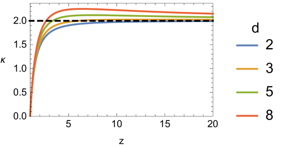
Figure 1: The exponent $\kappa$ of $\frac{\eta}{s}\sim T^{\kappa}$ as a function of $z$, with $\theta=0$ and $e^{2}=0$, for $d=2,3,5,8$. $\kappa$ can be greater than $2$ at finite $z$, when $d>2$.

In Figure 2, we plot the value of $\kappa$ as a function of $(z,\theta)$ in the allowed region with $d=2$. It is noticed that the value of $\kappa$ can be greater than $2$.

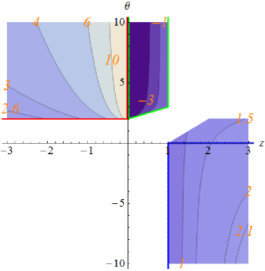
Figure 2: Contour plot of the exponent $\kappa$ of $\frac{\eta}{s}\sim T^{\kappa}$ over $(z,\theta)$ plane with $d=2$ and $e^{2}=0$. The left-upper region corresponds to $r\xrightarrow{IR}0$, which is divided into Region A (surrounded by red line) and Region B (surrounded by green line) as discussed in Section IV. The right-lower region corresponds to $r\xrightarrow{IR}+\infty$ and contains Region C (surrounded by blue line). The blank region violates the constraints (LABEL:constraint).

Up to now, we have only concentrated on the extremal IR geometry with hyperscaling violation by an analytical consideration, with a signal that the bound for $\kappa$ could be violated in some situations. It is still questionable if we could explicitly construct such kind of black hole solutions with UV completion at finite temperature. As a matter of fact, we point out with caution that model building may not be realized for all the parameters because the stability of the IR scaling solution and the existence of UV completion must be taken into account, as well as other natural requirements, such as $L^{2}>0,Q^{2}\geq 0$. Therefore, in next two sections we will address this issue by numerically solving the equations of motion and constructing explicit black hole solutions in which the new bound proposed in Hartnoll:2016tri is violated.

IV Isotropic dilaton-axion lattices with finite $(z,\theta)$

As explained in Section III, charge always reduces the exponent $\kappa$ for $\kappa>0$, so usually the charge plays no role in discussing the upper bound of $\kappa$. For simplicity, we continue to study on neutral backgrounds with relevant axion, which has already captured the power laws of $s\sim T^{\lambda}$ and $\frac{\eta}{s}\sim T^{\kappa}$. We immediately have $e^{2}=0$.

IV.1 Scaling solution and stability

We first consider the following 4-dimensional ED-Axion model

$$\mathcal{S}=\int dtd^{2}xdr\sqrt{-g}\left[R-\frac{c}{2}\left((\partial\phi)^{2}+e^{2\phi}\sum_{i=1,2}(\partial\chi_{i})^{2}\right)+n_{1}e^{\alpha\phi}\right],$$ (30)

in which we have chosen the potentials as $J(\phi)=ce^{2\phi},\,V(\phi)=n_{1}e^{\alpha\phi}$. Scaling solutions have been found in Donos:2014uba ; Gouteraux:2014hca . We deduce them in the hyperscaling violating ansatz (25) here. Looking for a solution of hyperscaling violation with relevant axions, we require that each term in the Lagrange should scale in the same way, i.e. $R\sim e^{2\phi}(\partial\chi_{i})^{2}\sim e^{\alpha\phi}$. So their exponents of $r$ satisfy equalities as

$$-\theta=2\phi_{1}+2-\theta=\alpha\phi_{1}.$$ (31)

We immediately have

$$\theta=\alpha,\quad\phi_{1}=-1.$$ (32)

Other parameters are deduced by solving the equations of motion. The result is

$$\begin{split}&z=\frac{\alpha^{2}-c-4}{2(\alpha-2)},\quad e^{\alpha\phi_{0}}L^{2}=\frac{((\alpha-6)(\alpha-2)+c)(-2\alpha+c+4)}{2(\alpha-2)^{2}n_{1}},\\ &e^{2\phi_{0}}k^{2}=\frac{((\alpha-6)(\alpha-2)+c)(c-(\alpha-2)\alpha)}{2(\alpha-2)^{2}c}.\end{split}$$ (33)

The above neutral solution is just the leading order solution with irrelevant current in Donos:2014uba ; Gouteraux:2014hca . It should give the same exponent $\kappa$ which only depends on the geometric parameters $(z,d_{\text{eff}})$. Besides, under the constraints (LABEL:constraint), $k^{2}\geq 0$ and $L^{2}>0$ are satisfied if $n_{1}>0$.

By using (32) and (LABEL:solution), the scaling behaviours (29) can be written in terms of $\alpha$ and $c$ as

$$s\sim T^{\frac{2(\alpha-2)^{2}}{-\alpha^{2}+c+4}},\quad\frac{\eta}{s}\sim T^{-\frac{(\alpha-8)\alpha-\sqrt{((\alpha-6)(\alpha-2)+c)\left(-7\alpha^{2}+8\alpha+9c+12\right)}+c+12}{-\alpha^{2}+c+4}}.$$ (34)

We now analyze the static modes by considering the following perturbation about the hyperscaling violating solution.

$$ds^{2}=L^{2}r^{\theta}\left(-\frac{(1+c_{t}r^{\delta})dt^{2}}{r^{2z}}+\frac{(1+c_{r}r^{\delta})dr^{2}+(1+c_{x}r^{\delta})(dx_{1}^{2}+dx_{2}^{2})}{r^{2}}\right),\quad e^{\phi}=e^{\phi_{0}}r^{-1}(1+c_{\phi}r^{\delta}).$$ (35)

By solving linearized perturbation equation, we find two pairs of modes after getting rid of the trivial modes . The two pairs of modes $\delta_{\pm}$ satisfying $\delta_{-}+\delta_{+}=\delta_{0}=2+z-\theta$. The first pair has $\delta^{(0)}_{-}=0$ and $\delta^{(0)}_{+}=\delta_{0}$ ($-c_{t}=c_{r}=r_{+}^{-\delta_{0}},c_{x}=c_{\phi}=0$), which correspond to rescaling of time and creating a small black hole (10) respectively. The other pair has

$$\delta_{\pm}^{(1)}=\frac{1}{2}\left(\delta_{0}\pm\frac{\sqrt{\delta_{0}(-\theta+2z-2)\left(\theta^{2}+8\theta-11\theta z+2z(9z-7)-4\right)}}{-\theta+2z-2}\right).$$ (36)

We point out that the relation $\delta_{+}>\delta_{-}$ is not implied for those two pairs of modes.

Since the location of the IR depends on $(z,\theta)$ or $(\alpha,c)$, we can not determine whether a mode is relevant or irrelevant from the sign of $\delta$. A plausible way is to check the sign of $\delta_{-}\delta_{+}$. If it is negative, then we always find that one of the pair of modes is irrelevant and stands for source, irrespective of the location of the IR. Here thanks to the constraints (LABEL:constraint), we have $\delta_{-}^{(1)}\delta_{+}^{(1)}=-\frac{2(z-1)(-\theta+z+2)(2z-\theta)}{-\theta+2z-2}\leq 0$, thus the scaling solution is RG stable.

The irrelevant mode among $\delta^{(1)}_{\pm}$ is adjusted to satisfy the boundary condition of $\phi$ on the UV boundary after UV completion; while the relevant mode of $\delta^{(0)}_{+}=\delta_{0}$ drives the extremal solution to a black hole with finite temperature. They are generally sufficient to construct a domain wall between AdS and hyperscaling violating geometry at finite temperature, which will be studied in the next subsection.

IV.2 UV completion and numerical results

As mentioned at the beginning of Section II, now we should do the UV completion to construct the bulk solution which is asymptotic to AdS. As explained in Charmousis:2010zz , the UV completing process can be achieved by demanding that $e^{\alpha\phi}\to 0$ in the UV of our previous solution and modifying the potential like $V(\phi)\to\frac{d(d+1)}{l^{2}}+n_{1}e^{\alpha\phi}$, where $l$ is the radius of AdS and is chosen to be 1 for convenience.

From solution (32), we have $e^{\alpha\phi}\propto r^{-\theta}$. The above UV completing process demands that $r^{-\theta}\to 0$ in the UV. For $r\xrightarrow{IR}0$, constraints (LABEL:constraint) lead to $\theta>0$, then the requirement $e^{\alpha\phi}\xrightarrow{UV}0$ is satisfied such that we can find a flow from $AdS_{4}$. On the other hand, for $r\xrightarrow{IR}+\infty$, we require $\theta<0$, which falls into a region of the constraints (LABEL:constraint), as shown in Figure 2. Notice that the UV completion process we adopt is not applicable to the region of $0\leq\theta<2$ . Nevertheless, we expect that other kind of UV completion is helpful, such as adopting a potential similar to the one in Ogawa:2011bz ; Huijse:2011ef . We expect to realize it in future.

Taking the different limits of temperature into account, we conclude that the allowed values for $(z,\theta)$ can be classified into three regions, as summarized in Table 1, among of which Region A and C have been mentioned in Donos:2014uba ; Gouteraux:2014hca . These three regions have been marked in Figure 2.

Regions	IR	Limit of $T$	$(z,\theta)$	$(\alpha,c)$	$\kappa$
Region A	$r\xrightarrow{IR}0$	$T\to 0$	$z<0\land\theta>2$	$2<\alpha<\sqrt{4+c}$	$\kappa>2$
Region B	$r\xrightarrow{IR}0$	$T\to+\infty$	$0<z\leq 1\land\theta>z+2$	$(2<\alpha\leq 3\land-\alpha^{2}+8\alpha-12<c<\alpha^{2}-4)$ $\lor(\alpha>3\land\alpha^{2}-2\alpha\leq c<\alpha^{2}-4)$	$\kappa\leq 0$
Region C	$r\xrightarrow{IR}+\infty$	$T\to 0$	$\theta<0\land z\geq 1$	$\alpha<0\land c\geq\alpha^{2}-2\alpha$	$0\leq\kappa<4$

Table 1: Three regions with different locations of IR and different limits of temperature when black holes become extremal. In the last column, we show the ranges of $\kappa$ by using (29).

As a result, we choose the following action with UV completion for Region A and Region B.

$$\mathcal{S}=\int dtd^{2}xdr\sqrt{-g}\left\{R+6+\frac{4c}{\alpha^{2}}\sinh(\frac{\alpha}{2}\phi)^{2}-\frac{c}{2}\left[(\partial\phi)^{2}+4\sinh^{2}(\phi)\sum_{i=1,2}(\partial\chi_{i})^{2}\right]\right\}.$$ (37)

The form of potential $V(\phi)$ imitates that in (6.1) in Kiritsis:2015oxa . When $\phi\to\infty$, we have $n_{1}=c/\alpha^{2}$.

The action admits an $AdS_{4}$ vacuum with unit radius. Since $V(\phi)=6+\frac{4c}{\alpha^{2}}\sinh(\frac{\alpha}{2}\phi)^{2}=6+c\phi^{2}+...$, the square of mass of dilaton is $-2$ on the boundary. Then we choose the conformal weight of its dual operator as $\Delta=1$.

The action does not allow a zero temperature solution with the near horizon geometry of $AdS_{2}\times R^{2}$ and $\phi=0$, since the term in front of axions, namely $\sinh^{2}(\phi)$, vanishes when the dilaton vanishes.

We adopt the following ansatz for numerical calculation.

$$ds^{2}=\frac{1}{u^{2}}\left(-(1-u)U(u)e^{-S(u)}dt^{2}+\frac{du^{2}}{(1-u)U(u)}+dx_{1}^{2}+dx_{2}^{2}\right),\quad\phi=\phi(u),\quad\chi_{1,2}=kx_{1,2}.$$ (38)

The AdS boundary is located at $u=0$. The horizon has been rescaled to $u=1$ such that the temperature and entropy density are $T=\frac{1}{4\pi}U(1)e^{-S(1)/2}$ and $s=4\pi$. The free energy density is $f=\epsilon-Ts$, where the energy density $\epsilon$ comes from the boundary expansion $(1-u)U(u)e^{-S(u)}=1+\cdots-\frac{\epsilon}{2}u^{3}+\cdots$. The dimensionless temperature, entropy density and free energy density are

$$\tilde{T}=\frac{T}{k},\quad\tilde{s}=\frac{s}{k^{2}},\quad\tilde{f}=\frac{f}{k^{3}},$$ (39)

where $k$ is the lattice number. We set the AdS boundary conditions as $U(0)=1,\,S(0)=0,\,\phi^{\prime\prime}(0)-\tau\phi^{\prime}(0)=0$, while impose the regularity boundary condition at horizon. As a result, each solution here is parameterized by two quantities, $(\tau,T/k)$, where $\tau$ is a dimensionless parameter specified by the AdS boundary condition of $\phi$.

Now we numerically build up the background solution and then solve the perturbation equation of $h(u)$ (7). Changing $T/k$ with a fixed $\tau$, we can numerically construct hyperscaling violating solutions in the IR only within a certain range of $\tau$. Finally we calculate $\eta/s$ numerically with the use of Eq. (18). We verify the power law behavior of $s$ and $\eta/s$ for some values of $(\alpha,c)$ in Region A and Region B, which is independent of the value for $\tau$. We find $\frac{\eta}{s}\leq\frac{1}{4\pi}$ in all the cases, and the equality holds up only when the black hole reaches the limit which is opposite to the extremal limit. We give some remarks as listed below.

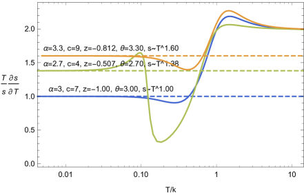
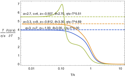
Figure 3: The scaling exponents of $s\sim T^{\lambda}$ (the left plot) and $\frac{\eta}{s}\sim T^{\kappa}$ (the right plot) as a function of $T/k$ in Region A. Solid lines represent the numerical results; dashed lines represent analytical results from (34). The extremal limit is at $T\to 0$.

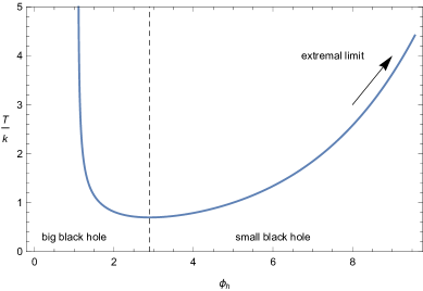
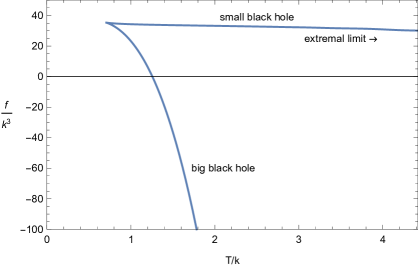
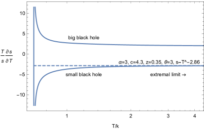
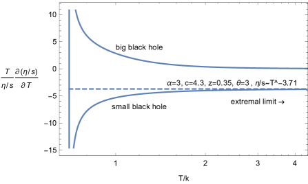
Figure 4: Numerical results in Region B with $\alpha=3$ and $\,c=4.3$. The left-upper plot shows $T/k$ as a function of $\phi_{h}=\phi(1)$. The right-upper plot shows the dimensionless free energy density $f/k^{3}$ as a function of $T/k$. The scaling exponents of $s\sim T^{\lambda}$ (the left-lower plot) and $\frac{\eta}{s}\sim T^{\kappa}$ (the right-lower plot) as a function of $T/k$. The extremal limit is at $T\to+\infty$ for small black hole.

• Figure 3 is a typical plotting for the temperature behavior of $s$ and $\eta/s$ in Region A. At low temperature, the scaling exponents of $s\sim T^{\lambda}$ and $\frac{\eta}{s}\sim T^{\kappa}$ through numerical calculation match the analytical results from Eq. (34) very well. In particular, the values of exponent $\kappa$ are greater than 2, in contrast to the results in Hartnoll:2016tri . At high temperature, the numerical results approach to $s\sim T^{2},\,\frac{\eta}{s}\sim 1$, which is the standard result for the usual AdS-Schwarzschild black hole.

• Figure 4 is a typical plotting for the temperature behavior of $s$ and $\eta/s$ in Region B. In the left-upper plot of Figure 4, we notice that above the minimal temperature $T_{min}$, there are two branches of black hole solutions, one corresponding to big black holes while the other to small black holes Gursoy:2008za ; Gursoy:2008bu ; Kiritsis:2015oxa . The $T\to+\infty$ limit of the big black hole is the AdS-Schwarzschild black hole. The extremal limit can be approached by heating the small black hole to $T\to+\infty$.

  The small black hole branch is thermodynamically unstable as expected, since its free energy density is greater than the one in big black hole branch with the same temperature, as shown in the right-upper plot of figure 4. Above certain a critical temperature $T_{c}>T_{min}$, the big black hole is thermodynamically dominated. While for $0<T<T_{c}$, the extremal limit with a periodical time of $t\sim t+iT^{-1}$ is dominated, which is the ground state of the system. A first order phase transition happens at $T_{c}$ between the ground state and the big black hole branch.

  Anyway, in the extremal limit we find that the scaling exponents from numerical calculation match the one of the hyperscaling violating solution (34), as shown in the bottom of Figure 4.

In the end of this section we turn to the temperature behavior of $s$ and $\eta/s$ for parameters in region C, in which the choice for UV completion is different. Since $\alpha<0$, if we expect that the term of $e^{\alpha\phi}$ in potential $V(\phi)$ is leading in the IR region, we need $\phi\to-\infty$. Thus we have to choose $J(\phi)=\frac{c}{4}\,\text{sech}^{2}(\phi)$ in order to reach the right hyperscaling violating solution above. Consequently, the modified action with UV completion for Region C is

$$\mathcal{S}=\int dtd^{2}xdr\sqrt{-g}\left\{R+6+\frac{4c}{\alpha^{2}}\sinh(\frac{\alpha}{2}\phi)^{2}-\frac{c}{2}\left[(\partial\phi)^{2}+\frac{1}{4}\,\text{sech}^{2}(\phi)\sum_{i=1,2}(\partial\chi_{i})^{2}\right]\right\}.$$ (40)

It should be noticed that though as $\phi\to-\infty$, $\text{sech}^{2}(\phi)\to 0$, we still have $\text{sech}^{2}(\phi)(\partial\chi_{i})^{2}\sim r^{-\alpha}\to+\infty$ to build up the ground state with relevant lattices.

Besides $AdS_{4}$ vacuum with unit radius, the action also admits a solution with extremal geometry of $AdS_{2}\times R^{2}$ and vanishing dilaton

$$ds^{2}=\frac{1}{3}ds^{2}_{AdS_{2}}+dx_{1}^{2}+dx_{2}^{2},\quad\chi_{i}=\sqrt{\frac{24}{c}}x_{i},\quad\phi=0.$$ (41)

Since $\frac{c}{8}\,\text{sech}^{2}(\phi)\sum_{i}(\partial\chi_{i})^{2}=6-6\phi^{2}+\cdots$, the square of effective mass of dilaton is $-(2+12/c)$, which violates the $AdS_{2}$ BF bound of $-\frac{3}{4}$. We expect that a condensation of dilaton occurs at relatively low temperature (but it is still at high temperature with respect to the emergence of hyperscaling violation).

Respect to the $AdS_{4}$ vacuum, the square of mass of dilaton is $-2$ as well. Here we choose the conformal weight of the dual operator of dilaton as $\Delta=2$ and demand its source to be zero by choosing one of the AdS boundary conditions as $\phi^{\prime}(0)=0$ for numerical convenience. The other boundary conditions are the same as those in Region A and B. Thus there is only one parameter $T/k$ remaining.

We numerically find that the dilaton condensates spontaneously at relatively low temperature. It leads to a second order phase transition between pure axion black hole and dilaton-axion black hole. By comparing the free energy, we find that the dilaton-axion black hole is thermodynamically dominated below the critical temperature. When we continuously drop down the temperature, the hyperscaling violating solution is approached and the power law is verified, as shown in Figure 5. We can see that $\kappa$ tends to the predicted number which is greater than 2.

Figure 5: The scaling exponents of $s\sim T^{\lambda}$ (the left plot) and $\frac{\eta}{s}\sim T^{\kappa}$ (the right plot) as a function of $T/k$ in Region C. The step at $T/k\approx 0.06$ results from the second order phase transition. The extremal limit is at $T\to 0$.

V Isotropic dilaton-linear axion lattices with infinite $(z,\theta)$: $\eta$-geometry

By rescaling the dilaton and parameters of (30) as in Donos:2014uba , we obtain the following action.

$$\mathcal{S}=\int dtd^{2}xdr\sqrt{-g}\left[R-\frac{1}{2}(\partial\phi)^{2}-\frac{1}{2}\sum_{i=1,2}(\partial\chi_{i})^{2}+n_{1}e^{\alpha\phi}\right],$$ (42)

where we have chosen the potentials as $J(\phi)=1,\,V(\phi)=n_{1}e^{\alpha\phi}$. It has a ground state which is conformal to $AdS_{2}\times R^{2}$ with lattices.

$$\begin{split}&ds^{2}=\frac{1}{r^{\bar{\eta}}}\left(L^{2}\frac{-dt^{2}+dr^{2}}{r^{2}}+dx_{1}^{2}+dx_{2}^{2}\right),\,e^{\phi}=r^{\phi_{1}},\,\chi_{1,2}=kx_{1,2},\\ &\bar{\eta}=\frac{2\alpha^{2}}{1-\alpha^{2}},\,k^{2}=n_{1}(1-\alpha^{2}),\,L^{2}=\frac{2(1+\alpha^{2})}{n_{1}(1-\alpha^{2})^{2}},\,\phi_{1}=\frac{2\alpha}{1-\alpha^{2}}.\end{split}$$ (43)

It corresponds to the situation of $z,\theta\to\infty$ while keeping $-\frac{\theta}{z}=\bar{\eta}$ fixed.

From $L^{2}>0,k^{2}>0$, we have $n_{1}>0,\alpha^{2}<1,\bar{\eta}>0$ and $r\xrightarrow{IR}+\infty$. We just choose $0<\alpha<1$ such that $\phi_{1}>0$ and $\phi\to+\infty$ at IR. Since $\bar{\eta}>0$, here the $\eta$-geometry can be obtained by taking the limit of $(z\to\mp\infty,\theta\to\pm\infty)$ in Region A or Region C.

Applying the following mode analysis

$$ds^{2}=\frac{1}{r^{\bar{\eta}}}\left[L^{2}\frac{-(1+c_{t}r^{\delta})dt^{2}+(1+c_{r}r^{\delta})dr^{2}}{r^{2}}+(1+c_{x}r^{\delta})(dx_{1}^{2}+dx_{2}^{2})\right],\,e^{\phi}=r^{\phi_{1}}(1+c_{\phi}r^{\delta}),$$ (44)

we find modes which are similar to Section IV. There are two pairs of modes which satisfy $\delta_{-}+\delta_{+}=1+\bar{\eta}$ after getting rid of the trivial modes . One pair has $\delta^{(0)}_{-}=0$ and $\delta^{(0)}_{+}=1+\bar{\eta}$ ($-c_{t}=c_{r}=r_{+}^{-1-\eta},c_{x}=c_{\phi}=0$), which correspond to rescaling of time and creating a small black hole with temperature $T\propto r_{+}^{-1}$. The other pair has

$$\delta^{(1)}_{\pm}=\frac{1}{2}\left(1+\bar{\eta}\pm\sqrt{(1+\bar{\eta})(9+\bar{\eta})}\right),$$ (45)

which satisfies $\delta^{(1)}_{-}\delta^{(1)}_{+}=-2(1+\bar{\eta})<0$. Then the scaling solution above are RG stable, for the same reason in Section IV.

As pointed out in Section III, the power law of $s$ and $\eta/s$ reads separately as

$$s\sim T^{\bar{\eta}},\quad\frac{\eta}{s}\sim T^{(1+\bar{\eta})\left(-1+\sqrt{1+\frac{8}{1+\bar{\eta}}}\right)}.$$ (46)

From $\bar{\eta}>0$, we have $2<\kappa<4$.

We adopt the following UV completing action.

$$\mathcal{S}=\int dtd^{2}xdr\sqrt{-g}\left\{R+6+\frac{4}{\alpha^{2}}\sinh(\frac{\alpha}{2}\phi)^{2}-\frac{1}{2}(\partial\phi)^{2}-\frac{1}{2}\sum_{i=1,2}(\partial\chi_{i})^{2}\right\}.$$ (47)

Similar to Region C in Section IV, the action admits $AdS_{4}$ vacuum with unit radius and $AdS_{2}\times R^{2}$ with radius of $1/\sqrt{3}$. The square of mass of dilaton is $-2$ and violates the $AdS_{2}$ BF of $-\frac{3}{4}$. We expect a condensation of dilaton.

Ansatz and the boundary conditions for numerical calculation are chosen to be the same as those in Region C. The hyperscaling violating solution is approached at low temperature and the power law is verified, as shown in Figure 6.

Figure 6: The scaling exponents of $s\sim T^{\lambda}$ (the left plot) and $\frac{\eta}{s}\sim T^{\kappa}$ (the right plot) as a function of $T/k$. The step at $T/k\approx 0.01$ results from the second order phase transition between pure axion black hole and dilaton-axion black hole. The extremal limit is at $T\to 0$.

VI Discussion and outlooks

VI.1 In comparison with the behavior of entanglement entropy

We have constructed specific models with the violation of the shear viscosity bound (2) in Section IV and V, which has been verified by numerical calculation. It becomes urgent to understand the underlying reasons leading to such violations. Apparently, the violation might be rooted in the nonzero exponent of hyperscaling violation $\theta$. But our analysis for higher dimension $d>2$ indicates that such kind of violation can occur even $\theta=0$, as shown in Figure 1.

As mentioned in the end of Subsection II.1, investigations of the behaviors of entanglement entropy give further constraint to the hyperscaling violating theories. We suggest that the bound violation may be related to the peculiar behavior of entanglement entropy in these theories. Explicitly,

• When $d_{\text{eff}}>1$ (containing Region C), we find $0\leq\kappa<4$, suggesting a new bound of 4 rather than 2. Within this region, the entanglement entropy is subject to the area law, implying that the dual local QFTs do not have large accidental degeneracies in low energy spectrum Huijse:2011ef . In addition, for $\eta$-geometry (LABEL:etageometry), the upper bound is 4 and the entanglement entropy satisfies the area law as well, under the condition that the width of the strip is large enough Liu:2013una .

• When $0\leq d_{\text{eff}}\leq 1$, we find $\kappa\leq 2$ from the power law (29), which just coincides with the bound (2). Within this region, the area law of entanglement entropy receives violations interpolating between the logarithmic and linear behavior Dong:2012se ; Huijse:2011ef . Especially, when $d_{\text{eff}}=1$, a logarithmic violation appears, signaling the existence of fermi surface; when $d_{\text{eff}}=0$, a linear violation appears and leads to a volume law, signaling an extensive ground state entropy. Recall that the known extremal IR geometries with nonvanishing lattices studied in Hartnoll:2016tri are $AdS_{2}\times R^{2}$, which belong to the case of $d_{\text{eff}}=0$, and the entanglement entropy shows volume law.

• When $d_{\text{eff}}<0$, we find $\kappa>2$ for $z<0\land e=0$ (containing Region A) and $\kappa\leq 0$ for $0<z\leq 1$ (containing Region B), which just violate the bound (2), neither more nor less, and suggesting the inexistence of the bound. Within this region, the entanglement entropy scales faster than the volume, which is not the behavior of QFT. Moreover, the stationary surface of entanglement entropy becomes a maximum, which suggests some instability of gravitational background Dong:2012se . So the violation of $0<\kappa<2$ in this region might be related to the abnormality of entanglement entropy and gravitational background.

From the analysis above, we give a conjecture that the bound of $\kappa$ depends on the behaviors of entanglement entropy, due to the different natures of ground states: when entanglement entropy shows area law, the bound is 4; when the area law have logarithmic to linear violation, the bound is 2; when the volume law is exceeded, then there is no bound.

VI.2 Conclusions and open questions

In this paper we have investigated the shear viscosity in a general holographic framework with hyperscaling violation. In the presence of isotropic and relevant lattices, we have demonstrated that the scaling relation in extremal IR region strongly constrains the mass term of graviton such that the ratio of shear viscosity to the entropy density always exhibits a power law behavior with temperature, $\eta/s\sim T^{\kappa}$. Significantly, we have found that in the EMD-Axion theory (19) the exponent $\kappa$ can be greater than 2 such that the bound (2) raised in Hartnoll:2016tri is violated. Our above observation has been verified by numerically constructing a large class of black hole solutions with UV completion in the EMD-Axion theory. On the other hand, when the axion is irrelevant, at subleading order, $k$ appears in the expression of $\eta/s$ as another scale and leads to a complicated behavior of temperature dependence (73) which is beyond the simple power law.

It is instructive to discuss the bound of entropy production rate in the holographic framework with hyperscaling violation, closely following the consideration presented in Hartnoll:2016tri . As analyzed in Section II, when breaking of translational invariance is relevant in the IR, operate $\hat{T}^{xy}$ acquires a scaling dimension of $\delta_{\hat{T}}$ in the IR, so as its dual source $\delta g_{xy}^{(0)}$ acquires $\delta_{0}-\delta_{\hat{T}}$, denoted as $[\delta g_{xy}^{(0)}]=\delta_{0}-\delta_{\hat{T}}$. Consider the source $\delta g_{xy}^{(0)}$ to be linear in time as proposed in Hartnoll:2016tri

$$\delta g_{xy}^{(0)}=tc^{(0)},$$ (48)

where $c^{(0)}$ is a time independent constant. Since $[t]=-[T]=-z$, then $[c^{(0)}]=\delta_{0}-\delta_{\hat{T}}+z$. On the other hand, from Eq.(17), we have $[\eta/s]=2(\delta_{\hat{T}}-\delta_{0})$. Then the equation about the rate of entropy density production

$$\frac{1}{T}\frac{d\log s}{dt}=\frac{\eta}{s}\left(\frac{c^{(0)}}{T}\right)^{2},$$ (49)

has scaling dimensions of zero on both sides, which is natural. Then the bound of entropy production rate is still allowable,

$$t_{\text{Pl}}\frac{d\log(s)}{dt}\gtrsim 1,$$ (50)

where $t_{\text{Pl}}=\frac{\hbar}{k_{B}T}$ is the ‘Planckian time’. Let us assume that temperature $T$ is still a dominating scale. Then $c^{(0)}=T^{\frac{\delta_{0}-\delta_{\hat{T}}}{z}+1}$ is the natural choice which satisfies the scaling dimension.

We have conjectured that the boundedness of $\kappa$ relates to the behavior of entanglement entropy. In particular, when the area law of entanglement entropy is satisfied, a higher bound of 4 for $\kappa$ has been suggested. The reason of the boundedness of $\kappa$ might be ascribed to the boundedness of scaling dimension of operator $\hat{T}^{xy}$.

Finally, a lot of open problems deserve for further investigation. Firstly, in this paper we have only considered the isotropic lattices due to the axion fields. In Section IV and V, we only do the calculation at the scaling solutions with vanishing current, and the UV complete solutions with (marginally) relevant current and (marginally) relevant lattices are worthy of investigation in future Gouteraux:2014hca ; Ling:2016yxy . On the other hand, the anisotropic situation is interesting as well, since an anisotropic scaling relation will emerge in the IR Donos:2014uba ; Donos:2014oha . Furthermore, by defining an effective (scaleless) mass of graviton, we expect that our scaling analysis on shear viscosity can be generalized to models in which the translational symmetry is broken by other effects, such as massive gravity Vegh:2013sk ; Andrade:2013gsa ; Alberte:2016xja , magnetic charge Liu:2016njg or disordering Hartnoll:2014cua ; Hartnoll:2015faa ; Hartnoll:2015rza , since the scaling relations emerged in the IR belong to one sort of hyperscaling violations.

Secondly, since other components of graviton are massive as well, Green functions associated with other components of energy-momentum tensor may exhibit similar scaling behaviors, then their susceptibilities, such as bulk viscosity, are expected to exhibit some power laws of temperature.

Thirdly, we stress that it is very crucial to understand the underlying reasons of boundedness or boundlessness of $\kappa$ in different regions. One may investigate it from the viewpoint of dimensional reduction, since the power law to the temperature may return to a more simple way in higher dimension. In EMD theories, the solutions of higher-dimensional theories reducing to $d_{\text{eff}}<0$ region are asymptotically flat p-branes Gouteraux:2011qh ; Gouteraux:2011ce . The boundlessness of $\kappa$ in this region may come from the absence of the scaling symmetry of AdS or Lifshitz in higher-dimensional spacetimes, although the exact dimensional reduction of the EMD-Axion theories is not clear yet.

The violation of the area law of entanglement entropy is related to the bound for entanglement entropy production rate Acoleyen:2013era , which has been studied during thermalization in holographic system Liu:2013qca ; Alishahiha:2014cwa . The relation between the shear viscosity bound and entanglement entropy calls for further investigation.

Appendix A Shear viscosity with (marginally) relevant axion

In this appendix we derive the shear viscosity $\eta$ through the retarded Green function explicitly. We will show that the result is consistent with that from the scale analysis (17). We start from the shear perturbation equation in hyperscaling violating metric (10) which reads as

$$\partial_{r}(r^{1-\delta_{0}}f(r)\partial_{r}h(r))+(\frac{r^{2z-\delta_{0}-1}\omega^{2}}{f(r)}-M^{2}L^{2}r^{-\delta_{0}-1})h(r)=0,$$ (51)

where

$$f(r)=1-\left(\frac{r}{r_{+}}\right)^{\delta_{0}},~{}~{}~{}~{}\delta_{0}:=d+z-\theta.$$ (52)

Note that we have used $m(r)^{2}=M^{2}r^{-\frac{2\theta}{d}}$ as discussed in Section II. We remind that $M^{2}\geq 0,L^{2}>0$ and temperature is $T=|\delta_{0}|r_{+}^{-z}/(4\pi)$.

To solve this equation, we change it into a transparent form by defining

$$\xi:=\frac{r^{\delta_{0}}}{r_{+}^{\delta_{0}}}\,,~{}~{}~{}~{}~{}a:=\frac{1}{2}\left(1-\sqrt{1+\left(\frac{2ML}{\delta_{0}}\right)^{2}}\right),$$ (53)

where $a\leq 0$. The new coordinate $\xi$ covers the region $1\geq\xi\geq 0$, with the horizon at $\xi=1$ and the boundary at $\xi=0$. Now, the perturbation equation (51) can be rewritten as

$$(1-\xi)\partial^{2}_{\xi}h(\xi)-\partial_{\xi}h(\xi)+\left(\frac{\xi^{\frac{2z}{\delta_{0}}-2}}{1-\xi}\left(\frac{\omega}{4\pi T}\right)^{2}-\frac{a(a-1)}{\xi^{2}}\right)h(\xi)=0.$$ (54)

As we will see below, the term of $\omega^{2}$ is not important for calculating the viscosity. With regularity condition at horizon, the zero frequency solution $h_{0}(\xi)$ can be obtained as

$$h_{0}(\xi)=\,\xi^{a}\,_{2}F_{1}(a,a;2a;\xi)-\frac{\Gamma(1-a)^{2}\Gamma(2a)}{\Gamma(2-2a)\Gamma(a)^{2}}\,\xi^{1-a}\,_{2}F_{1}(1-a,1-a;2-2a;\xi),$$ (55)

where ${}_{2}F_{1}(a,b;c;z)$ is the Gaussian hypergeometric function. Especially, at the horizon we have

$$h_{0}(1)=\frac{\pi^{2}\csc^{2}(\pi a)}{\Gamma(1-2a)\Gamma(a)^{2}},$$ (56)

while on the boundary, $h_{0}(\xi)$ behaves as

$$h_{0}(\xi\rightarrow 0)=\xi^{a}+\cdots-\frac{\Gamma(1-a)^{2}\Gamma(2a)}{\Gamma(2-2a)\Gamma(a)^{2}}\,\xi^{1-a}+\cdots,$$ (57)

which is the explicit form of (13).

We next introduce the in-falling boundary condition and expand the solution in power of the frequency as

$$\begin{split}h(\xi)&=(1-\xi)^{\frac{-i\omega}{4\pi T}}h_{0}(\xi)(1+i\omega H(\xi)+\mathcal{O}(\omega)^{2})\\ &=h_{0}(\xi)(1+i\omega\tilde{H}(\xi)+\mathcal{O}(\omega)^{2}),\end{split}$$ (58)

where $H(\xi)$ is regular at the horizon and $\tilde{H}(\xi)=H(\xi)-\frac{\ln(1-\xi)}{4\pi T}$. Then, substituting the above expansion into (54), we derive a conservation equation up to the first order of $\omega$

$$\partial_{\xi}(h_{0}(\xi)^{2}(1-\xi)\partial_{\xi}\tilde{H}(\xi))=0.$$ (59)

Now we evaluate the conserved quantity $h_{0}(\xi)^{2}(1-\xi)\partial_{\xi}\tilde{H}(\xi)$ at the horizon, leading to

$$\partial_{\xi}\tilde{H}(\xi)=\frac{h_{0}(1)^{2}}{4\pi T(1-\xi)h_{0}(\xi)^{2}}.$$ (60)

This result gives the asymptotic behavior of $\tilde{H}(\xi)$ on the boundary

$$\tilde{H}(\xi\rightarrow 0)=C+\frac{h_{0}(1)^{2}}{4\pi T(1-2a)}\xi^{-2a+1}+\cdots,$$ (61)

where (57) has been used and $C$ is an integration constant. Finally, we have the asymptotic behavior of $h(\xi)$ on the boundary

$$h(\xi\rightarrow 0)=\xi^{a}+\cdots+\left(i\omega\frac{h_{0}(1)^{2}}{(1-2a)4\pi T}-\frac{\Gamma(1-a)^{2}\Gamma(2a)}{\Gamma(2-2a)\Gamma(a)^{2}}\right)\xi^{-a+1}+\cdots+\mathcal{O}(\omega^{2}).$$ (62)

Next we derive the viscosity from the imaginary part of the retarded Green function in (16). To do that we change the coordinate $\xi$ in (62) back to the original one in (53). We find the viscosity takes the following form in hyperscaling violating geometry

$$\eta_{\text{HV}}=\lim_{\omega\to 0}\frac{\text{Im}\,\mathcal{G}^{R}_{\hat{T}^{xy},\hat{T}^{xy}}(\omega,k=0)}{\omega}=\frac{h_{0}(1)^{2}}{b|\delta_{0}|(1-2a)}\left(\frac{4\pi T}{|\delta_{0}|}\right)^{-1+\frac{\delta_{0}}{z}\sqrt{1+\left(\frac{2ML}{\delta_{0}}\right)^{2}}},$$ (63)

where (11) has been used and $h_{0}(1)$ is given by (56).

On the other hand, given the entropy density in (11), thus we have

$$\frac{\eta_{\text{HV}}}{s}=\frac{h_{0}(1)^{2}}{4\pi b|\delta_{0}|(1-2a)}\left(\frac{4\pi T}{|\delta_{0}|}\right)^{\frac{\delta_{0}}{z}\left(-1+\sqrt{1+\left(\frac{2ML}{\delta_{0}}\right)^{2}}\right)}.$$ (64)

By using the UV-IR matching explained in Section II, we have $\frac{\eta}{s}\propto\frac{\eta_{\text{HV}}}{s}$. Therefore, our result obtained from Green function confirms the temperature behavior of $\eta/s$ given by the scaling analysis (17). Besides, if hyperscaling violation is also valid in the UV, i.e. without the AdS-UV completion, the holographic renormalization for a certain hyperscaling violating theory is needed, and the constant $b$ in the expansion (16) could be determined, at least for EMD theory Chemissany:2014xpa ; Taylor:2015glc . While, for EMD-Axion theory, the holographic renormalization may be very different, since the scaling dimension of $\hat{T}^{xy}$ is $\delta_{\hat{T}}$ now, which can deviate from the usual value of $\delta_{0}=d-\theta+z$ in the translational invariance cases Chemissany:2014xpa ; Taylor:2015glc .

Appendix B Shear viscosity with irrelevant axion

We are going to study $\eta/s$ on EMD-Axion model with irrelevant axion at subleading order. We will consider the perturbation of $h_{0}(r)$ and find the solution up to ${\cal O}(k^{2})$ and then derive the temperature dependence of $\eta/s$. Finally, we come to numerical calculation to justify our formula.

B.1 Analytical consideration and approximation

We rewrite the action of EMD-Axion model in which the hyperscaling violation is allowable Gouteraux:2014hca

$$\mathcal{S}=\int dtd^{d}xdr\sqrt{-g}\left[R+V_{0}e^{\alpha\phi}-\frac{1}{2}(\partial\phi)^{2}-\frac{1}{2}e^{\beta\phi}\sum_{i=1}^{d}(\partial\chi_{i})^{2}-\frac{e^{\gamma\phi}}{4}F^{2}\right].$$ (65)

The black hole solution deformed by irrelevant axion up to ${\cal O}(k^{2})$ has the following form

$$\begin{split}&ds^{2}=r^{\frac{2\theta}{d}}\left[-\frac{L_{t}^{2}f(r)dt^{2}}{r^{2z}}(1+k^{2}S_{t}(r))+\frac{L_{r}^{2}dr^{2}}{r^{2}f(r)}(1+k^{2}S_{r}(r))+\frac{L_{x}^{2}\sum_{i=1}^{d}dx_{i}^{2}}{r^{2}}(1+k^{2}S_{x}(r))\right],\\ &A=Qr^{\zeta-z}f(r)dt,\quad e^{\phi}=e^{\phi_{0}}r^{\phi_{1}}(1+k^{2}S_{\phi}(r)),\quad\chi_{i}=kx_{i},\end{split}$$ (66)

where

$$\phi_{1}^{2}=\frac{2(d-\theta)((z-1)d-\theta)}{d},\quad\alpha\phi_{1}=-\frac{2\theta}{d},\quad L_{r}^{2}e^{\alpha\phi_{0}}=\frac{(d+z-\theta-1)(d+z-\theta)}{n_{1}}.$$ (67)

The axion back-reacts to the metric and the dilaton with modes $S_{J}(r)$ for $J=\{t,r,x,\phi\}$. $S_{J}(r)$ satisfy some nonhomogeneous second order differential equations with sources of axion. Since there are freedom for redefinition of $r$ as in usual mode analysis, we can choose the gauge condition of $S_{t}(r)=0$. Near the boundary, the asymptotic behaviors of other modes are $S_{J}(r)=s_{J,0}r^{\Delta}+s_{J,1}r^{\Delta}\left(\frac{r}{r_{+}}\right)^{\delta_{0}}+\cdots$, where $\Delta=2+\beta\phi_{1}$. Axion is irrelevant when $\delta_{0}\Delta<0$. At the horizon, $S_{r}(r_{+})=S_{x}(r_{+})=S_{\phi}(r_{+})=S_{r}^{\prime}(r_{+})=0$ are required to eliminate other modes. Then the temperature is $T=\frac{|\delta_{0}|L_{t}}{4\pi L_{r}}r_{+}^{-z}$. We have maintained the freedom of rescaling coordinates into $\{L_{t},L_{r},L_{x}\}$ for the convenience of numerical calculation in the next subsection.

Like the case in Appendix A, we can rewrite the shear perturbation equation for $\omega=0$ in (7) with coordinate $\xi=\left(r/r_{+}\right)^{\delta_{0}}$ and solve for $h_{0}(\xi)$ with $k^{2}$ expansion

$$h_{0}(\xi)=h_{0}^{(0)}(\xi)+k^{2}h_{0}^{(1)}(\xi)+\cdots,$$ (68)

which are subject to the following iterative equations

$$\partial_{\xi}((1-\xi)\partial_{\xi}h_{0}^{(0)}(\xi)) = 0,$$ (69)

$$\partial_{\xi}((1-\xi)\partial_{\xi}h_{0}^{(1)}(\xi)) = \frac{L_{r}^{2}}{\delta_{0}^{2}L_{x}^{2}}e^{\beta\phi_{0}}r_{+}^{\Delta}\xi^{b-2}h_{0}^{(0)}(\xi)-S_{1}(\xi)\partial_{\xi}h_{0}^{(0)}(\xi)+S_{2}(\xi)\partial_{\xi}^{2}h_{0}^{(0)}(\xi),$$ (70)

where $S_{1}(\xi)$ and $S_{2}(\xi)$ are some linear combinations of $S_{J}$ and their derivatives and $b=\Delta/\delta_{0}<0$. We expect ${\cal O}(k^{2})$ approximation is enough to fit the low temperature dependence of $\eta/s$ when $k$ is small. The solution to Eq.(69) which is regular at the horizon is $h_{0}^{(0)}(\xi)=C$, with $C$ being a constant. Plug it into (70), we find that the terms of $S_{1}(\xi)$ and $S_{2}(\xi)$ vanish and the horizon-regular solution is $h_{0}^{(1)}(\xi)=C\frac{L_{r}^{2}}{\delta_{0}^{2}L_{x}^{2}}e^{\beta\phi_{0}}r_{+}^{\Delta}\frac{\xi^{b}+b(B_{\xi}(b+1,0)+\log(1-\xi))}{(b-1)b}$. So the full solution up to ${\cal O}(k^{2})$ is

$$h_{0}(\xi)=C\left[1+K^{2}r_{+}^{\Delta}\frac{\xi^{b}+b(B(\xi;b+1,0)+\log(1-\xi))}{(b-1)b}\right]\quad\text{with}\quad K^{2}=\frac{k^{2}L_{r}^{2}}{\delta_{0}^{2}L_{x}^{2}}e^{\beta\phi_{0}},$$ (71)

where $B(\xi;b+1,0)$ is the incomplete beta function whose series definition is $B(\xi;b+1,0)=\sum_{i=0}^{\infty}\frac{\xi^{b+1+i}}{b+1+i}$. Formula (71) can tell us how temperature affects the value of $h_{0}(\xi)$ at horizon, namely $h_{0}(1)$. Let us focus on the cases in which the extremal limit is at $T\to 0$. At low temperature, hyperscaling violation emerges in the IR and (LABEL:HVirrelevant) is valid only within an interval between $r_{i}$ and $r_{+}$. It connects to AdS deformed by matter fields near an intermediate scale $r_{i}$. The constant $C$ can be determined by evaluating $h_{0}$ at $r_{i}$ as

$$h_{0}(\xi_{i})=\Gamma$$ (72)

where $\xi_{i}=(r_{i}/r_{+})^{\delta_{0}}$ and $\Gamma$ can be understood as the tunnelling rate. Such an idea was proposed in Hartnoll:2016tri , while here we just apply it to the intermediate scale $r_{i}$. When temperature is much lower than other scales, it becomes not important to the RG flow from AdS to hyperscaling violation. The tunnelling rate, which characterizes how $h_{0}$ decays from the conformal boundary to $r_{i}$, becomes insensitive to temperature and is expected to go to a constant at low temperature. So temperature mainly controls $h_{0}$ by varying $r_{+}$ in (71). Although we have no general analytical solution with UV completion and can not determine $C,\,\Gamma$ or $r_{i}$ analytically, we can estimate them by numerical fitting in the next subsection.

By working out $C$ from (72), we obtain the value of $h_{0}$ at horizon as

$$h_{0}(\xi=1) = \Gamma\frac{(b-1)b-K^{2}r_{+}^{\Delta}\left(bH_{b}-1\right)}{(b-1)b+K^{2}r_{+}^{\Delta}\left[\xi_{i}^{b}+b\left(B_{\xi_{i}}(b+1,0)+\log\left(1-\xi_{i}\right)\right)\right]}$$ (73)

$$\approx \Gamma\left[1+\frac{K^{2}}{1-b}\left(r_{i}^{\Delta}+\frac{bH_{b}-1}{b}r_{+}^{\Delta}+\frac{r_{i}^{\Delta+\delta_{0}}}{b+1}r_{+}^{-\delta_{0}}+\cdots\right)\right],$$ (74)

where $H_{b}$ is the $b^{\text{th}}$ harmonic number. Then $\eta/s$ can be obtained directly by the weaker horizon formula (18). As asserted in the main text, in the expansion (74), the leading term is constant $\Gamma$ while scales $k^{2}$ and $e^{\phi_{0}}$ appear at the subleading term. We find that when the axion becomes irrelevant, the temperature dependence of $\eta/s$ up to ${\cal O}(k^{2})$ is more complicated than the case with (marginally) relevant axion. The reason can be seen by rewriting the mass-like term as

$$K^{2}r_{+}^{\Delta}\propto\left\{\begin{array}[]{lll}k^{2}e^{\beta\phi_{0}},&\text{for}&\Delta=0,\\ \left(\frac{k}{T^{1/z}}\right)^{2}\left(\frac{e^{\phi_{0}}}{T^{\phi_{1}/z}}\right)^{\beta},&\text{for}&\Delta\neq 0,\end{array}\right.$$ (75)

where quantities $\{L_{t},L_{r},L_{x}\}$ have been absorbed in $\{T,e^{\phi_{0}},k\}$ by coordinate transformations. When axion is (marginally) relevant, namely, $\Delta=0$, the other two scales $k$ and $e^{\phi_{0}}$ are combined into a scaleless quantity $M^{2}$ and only enter the scaling dimension (15). While, when axion is irrelevant, namely, $\Delta\delta_{0}<0$, they enter $m(r)^{2}$ with a form coupling to $T$ and lead to a complicated behavior of temperature dependence. Nevertheless, since axion is irrelevant, $\eta/s$ is finally expected to converge to a nonzero constant at extremal low temperature Hartnoll:2016tri . But, as seen from the expansion (74), the rate of convergence behaves like $T^{\min(\frac{-\Delta}{z},\frac{\delta_{0}}{z})}$ that could happen to be too slow to be observed numerically. The full expression (73) goes beyond the simple power law and seems hard to obtain through scaling analysis.

In Eq.(73), there are two parameters $\{\Gamma,r_{i}\}$ which should be given by fitting in the next subsection.

B.2 Numerical calculation and fitting

Now we conduct numerical calculation for neutral background with positive specific heat and irrelevant axion. The allowed parameter space is $z=1,\theta<0$ and $\Delta<0$ Gouteraux:2014hca . Cases of $z\neq 1$ can be constructed with (marginally) relevant current Gouteraux:2014hca . For generality, we retain the freedom of $z$ in the following discussion. Different from subsection IV.2, the UV completive form of $V(\phi)$ is chosen as

$$V(\phi)=(d(d+1)-2n_{1})\left(1-\tanh^{2}(\alpha\phi)\right)+2n_{1}\cosh(\alpha\phi),\quad n_{1}=\frac{d\left(2\alpha^{2}+2\alpha^{2}d+1\right)}{6\alpha^{2}}$$ (76)

for the purpose that $V(\phi)$ approaches to $n_{1}e^{\alpha\phi}$ quickly even when $\phi$ is not too large. Other settings in (19) are $J(\phi)=e^{\beta\phi},Z(\phi)=0$ and $c=1$. The ansatz for the metric in numerical calculation is similar to (38)

$$ds^{2}=\frac{1}{u^{2}}\left(-\frac{(1-u)U(u)}{S(u)}dt^{2}+\frac{du^{2}}{(1-u)U(u)}+\sum_{i=1}^{d}dx_{i}^{2}\right),\quad\phi=\phi(u),\quad\chi_{i}=kx_{i}.$$ (77)

When $\phi$ is small, expansion $V(\phi)=d(d+1)+d\phi^{2}+\cdots$ gives boundary expansion $\phi=\tau u+\cdots+\nu u^{d}+\cdots$. The boundary conditions are $U(0)=1,\,S(0)=1,\,\phi^{\prime}(0)=\tau$ at $u=0$ and regular conditions at $u=1$. In this coordinate, temperature and entropy density are $T=\frac{U(1)}{4\pi\sqrt{S(1)}}$ and $s=4\pi$. The dimensions of $T$ and $k$ are chosen to be cancelled by unit $\tau$. Then our numerical solutions are parameterized by two dimensionless quantities $\{\frac{T}{\tau},\frac{k}{\tau}\}$.

When lowering down $T/\lambda$, we fix $k/\lambda$. Hyperscaling violation emerges near the horizon $u\to 1$ at low temperature. It can be directly observed by coordinate transformation $u\to r^{1-\frac{\theta}{d}}/\tau,\,t\to t/\tau,\,x_{i}\to x_{i}/\tau$ to the one used in (LABEL:HVirrelevant). Then we know the location of horizon is $r_{+}=\tau^{\frac{d}{d-\theta}}$ and the parameters accordingly transform as $T\to\tau T,\,k\to\tau k$ and $s\to\tau^{d}s$. It means that the temperature, lattices scale and entropy density in coordinate (LABEL:HVirrelevant) are equal to the dimensionless ones in (77). Then the quantities $\{L_{r}^{2},L_{t}^{2},e^{\phi_{0}}\}$ in (LABEL:HVirrelevant) can be extracted from ansatz (77) as

$$L_{r}^{2}=\frac{|d-\theta||\delta_{0}|}{dU(1)}\tau^{\frac{-2\theta}{d-\theta}},\quad L_{t}^{2}=\frac{|d-\theta|U(1)}{d|\delta_{0}|S(1)}\tau^{\frac{2d(z-1)}{d-\theta}},\quad e^{\phi_{0}}=e^{\phi(1)}\tau^{\frac{-d\phi_{1}}{d-\theta}}.$$ (78)

Then $K^{2}$ can be calculated by using (71).

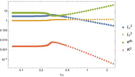
Figure 7: The exponent $\lambda$ of $s\sim T^{\lambda}$ as a function of $T/\tau$ is shown in the left plot, where solid line denotes numerical result and dashed line denotes analytical result. Quantities $\{L_{r}^{2},L_{t}^{2},e^{\phi_{0}},K^{2}\}$ as a function of $T/\tau$ is shown in the right plot. The parameters are $d=2,\,\alpha=0.8,\,\beta=-1$ and $k/\tau=0.5$, then $z=1,\,\theta=-3.56$ and $\Delta=-2.44$.

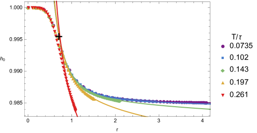
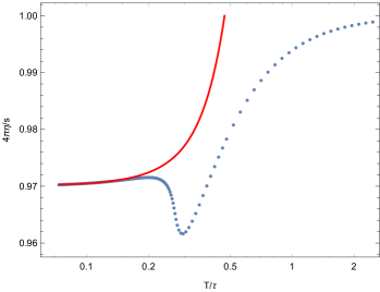
Figure 8: $h_{0}(r)$ at various temperatures are shown in the left plot, where the numerical solutions are denoted by points and the results from fitting (71) are denoted by lines. $4\pi\eta/s$ as a function of $T/\tau$ is shown in the right plot, where blue points denote numerical result and red line denotes result from fitting (73). The fitting values of $\{\Gamma,r_{i}\}$ are marked by the black cross in the left plot.

We demonstrate our numerical calculation in $d=2$. The exponent $\lambda$ of $s\sim T^{\lambda}$ converges to $\frac{d-\theta}{z}$ at low $T/\tau$, as shown in the left plot of Figure 7. Quantities $\{L_{r}^{2},L_{t}^{2},e^{\phi_{0}},K^{2}\}$ go to constants at low $T/\tau$ as well, as shown in the right plot of Figure 7. Numerical solutions for $h_{0}(r)$ at different temperatures $T/\tau$ are plotted in the left of Figure 8. As expected, $h_{0}(r\lesssim 1)$ in the UV region becomes insensitive to $T/\tau$ when $T/\tau$ is small, while in the IR region $h_{0}(r\gtrsim 1)$ matches well with (71) where constant $C$ is the fitting parameter. The temperature behavior of $\eta/s$ is illustrated in the right plot of Figure 8. From this figure we notice that $\eta/s$ falls off quickly at first which is controlled by AdS deformed by axion. It goes to the minimum at $T/\tau\approx 0.29$ then rises again because the axion begins to be suppressed in the IR, which is also hinted by the peak of $K^{2}$ at $T/\tau\approx 0.29$ in Figure 7. When $T/\tau\approx 0.2$, hyperscaling violation begins to emerge and then $\eta/s$ begins to satisfy (73). To fit the numerical data of $\eta/s$ by using (73), we fix the value of $K^{2}$ at lowest $T/\tau$ and select the fitting interval as $T/\tau<0.116$. $\{\Gamma,r_{i}\}$ are the two fitting parameters, whose fitting values are marked in the left plot of Figure 8. The fitting curves match the data well when $T/\tau$ is low. We remark that the fitting values of $\{\Gamma,r_{i}\}$ are sensitive to the fitting interval of $T/\tau$ but satisfy (72) pretty well at low $T/\tau$.

References

- (1) P. Kovtun, D. T. Son and A. O. Starinets, “Viscosity in strongly interacting quantum field theories from black hole physics,” Phys. Rev. Lett. 94, 111601 (2005) [hep-th/0405231].
- (2) D. Mateos and D. Trancanelli, “The anisotropic N=4 super Yang-Mills plasma and its instabilities,” Phys. Rev. Lett. 107, 101601 (2011) [arXiv:1105.3472 [hep-th]].
- (3) D. Mateos and D. Trancanelli, “Thermodynamics and Instabilities of a Strongly Coupled Anisotropic Plasma,” JHEP 1107, 054 (2011) [arXiv:1106.1637 [hep-th]].
- (4) A. Rebhan and D. Steineder, “Violation of the Holographic Viscosity Bound in a Strongly Coupled Anisotropic Plasma,” Phys. Rev. Lett. 108, 021601 (2012) [arXiv:1110.6825 [hep-th]].
- (5) X. H. Ge, Y. Ling, C. Niu and S. J. Sin, “Thermoelectric conductivities, shear viscosity, and stability in an anisotropic linear axion model,” Phys. Rev. D 92, no. 10, 106005 (2015) [arXiv:1412.8346 [hep-th]].
- (6) R. A. Davison and B. Gout raux, “Momentum dissipation and effective theories of coherent and incoherent transport,” JHEP 1501, 039 (2015) [arXiv:1411.1062 [hep-th]].
- (7) S. A. Hartnoll, D. M. Ramirez and J. E. Santos, “Entropy production, viscosity bounds and bumpy black holes,” JHEP 1603, 170 (2016) [arXiv:1601.02757 [hep-th]].
- (8) L. Alberte, M. Baggioli and O. Pujolas, “Viscosity bound violation in holographic solids and the viscoelastic response,” arXiv:1601.03384 [hep-th].
- (9) P. Burikham and N. Poovuttikul, “Shear viscosity in holography and effective theory of transport without translational symmetry,” arXiv:1601.04624 [hep-th].
- (10) H. S. Liu, H. Lu and C. N. Pope, “Magnetically-Charged Black Branes and Viscosity/Entropy Ratios,” arXiv:1602.07712 [hep-th].
- (11) S. A. Hartnoll and D. M. Hofman, “Locally Critical Resistivities from Umklapp Scattering,” Phys. Rev. Lett. 108, 241601 (2012) [arXiv:1201.3917 [hep-th]].
- (12) M. Blake, D. Tong and D. Vegh, “Holographic Lattices Give the Graviton an Effective Mass,” Phys. Rev. Lett. 112, no. 7, 071602 (2014) [arXiv:1310.3832 [hep-th]].
- (13) S. Kachru, X. Liu and M. Mulligan, “Gravity duals of Lifshitz-like fixed points,” Phys. Rev. D 78, 106005 (2008) [arXiv:0808.1725 [hep-th]].
- (14) M. Taylor, “Non-relativistic holography,” arXiv:0812.0530 [hep-th].
- (15) S. S. Gubser and A. Nellore, “Ground states of holographic superconductors,” Phys. Rev. D 80, 105007 (2009) [arXiv:0908.1972 [hep-th]].
- (16) S. Sachdev, “Quantum Phase Transitions,” 2nd Edition, Cambridge University Press (2011).
- (17) S. S. Gubser and F. D. Rocha, “Peculiar properties of a charged dilatonic black hole in ,” Phys. Rev. D 81, 046001 (2010) [arXiv:0911.2898 [hep-th]].
- (18) M. Cadoni, G. D’Appollonio and P. Pani, “Phase transitions between Reissner-Nordstrom and dilatonic black holes in 4D AdS spacetime,” JHEP 1003, 100 (2010) [arXiv:0912.3520 [hep-th]].
- (19) K. Goldstein, S. Kachru, S. Prakash and S. P. Trivedi, “Holography of Charged Dilaton Black Holes,” JHEP 1008, 078 (2010) [arXiv:0911.3586 [hep-th]].
- (20) C. Charmousis, B. Goutéraux, B. S. Kim, E. Kiritsis and R. Meyer, “Effective Holographic Theories for low-temperature condensed matter systems,” JHEP 1011, 151 (2010) [arXiv:1005.4690 [hep-th]].
- (21) E. Perlmutter, “Domain Wall Holography for Finite Temperature Scaling Solutions,” JHEP 1102, 013 (2011) [arXiv:1006.2124 [hep-th]].
- (22) B. Goutéraux, J. Smolic, M. Smolic, K. Skenderis and M. Taylor, “Holography for Einstein-Maxwell-dilaton theories from generalized dimensional reduction,” JHEP 1201, 089 (2012) [arXiv:1110.2320 [hep-th]].
- (23) B. Goutéraux and E. Kiritsis, “Generalized Holographic Quantum Criticality at Finite Density,” JHEP 1112, 036 (2011) [arXiv:1107.2116 [hep-th]].
- (24) N. Iizuka, N. Kundu, P. Narayan and S. P. Trivedi, “Holographic Fermi and Non-Fermi Liquids with Transitions in Dilaton Gravity,” JHEP 1201, 094 (2012) [arXiv:1105.1162 [hep-th]].
- (25) N. Ogawa, T. Takayanagi and T. Ugajin, “Holographic Fermi Surfaces and Entanglement Entropy,” JHEP 1201, 125 (2012) [arXiv:1111.1023 [hep-th]].
- (26) L. Huijse, S. Sachdev and B. Swingle, “Hidden Fermi surfaces in compressible states of gauge-gravity duality,” Phys. Rev. B 85, 035121 (2012) [arXiv:1112.0573 [cond-mat.str-el]].
- (27) X. Dong, S. Harrison, S. Kachru, G. Torroba and H. Wang, “Aspects of holography for theories with hyperscaling violation,” JHEP 1206, 041 (2012) [arXiv:1201.1905 [hep-th]].
- (28) M. Alishahiha and H. Yavartanoo, “On Holography with Hyperscaling Violation,” JHEP 1211, 034 (2012) [arXiv:1208.6197 [hep-th]].
- (29) J. Bhattacharya, S. Cremonini and A. Sinkovics, “On the IR completion of geometries with hyperscaling violation,” JHEP 1302, 147 (2013) [arXiv:1208.1752 [hep-th]].
- (30) B. Goutéraux and E. Kiritsis, “Quantum critical lines in holographic phases with (un)broken symmetry,” JHEP 1304, 053 (2013) [arXiv:1212.2625 [hep-th]].
- (31) E. Kiritsis and J. Ren, “On Holographic Insulators and Supersolids,” JHEP 1509, 168 (2015) [arXiv:1503.03481 [hep-th]].
- (32) A. Donos and J. P. Gauntlett, “Novel metals and insulators from holography,” JHEP 1406, 007 (2014) [arXiv:1401.5077 [hep-th]].
- (33) B. Goutéraux, “Charge transport in holography with momentum dissipation,” JHEP 1404, 181 (2014) [arXiv:1401.5436 [hep-th]].
- (34) J. Zaanen, Y. W. Sun, Y. Liu and K. Schalm, “Holographic Duality in Condensed Matter Physics.”
- (35) M. Edalati, J. F. Pedraza and W. Tangarife Garcia, “Quantum Fluctuations in Holographic Theories with Hyperscaling Violation,” Phys. Rev. D 87, no. 4, 046001 (2013) [arXiv:1210.6993 [hep-th]].
- (36) A. Donos, B. Goutéraux and E. Kiritsis, “Holographic Metals and Insulators with Helical Symmetry,” JHEP 1409, 038 (2014) [arXiv:1406.6351 [hep-th]].
- (37) A. Donos and S. A. Hartnoll, “Universal linear in temperature resistivity from black hole superradiance,” Phys. Rev. D 86, 124046 (2012) [arXiv:1208.4102 [hep-th]].
- (38) T. Faulkner, H. Liu, J. McGreevy and D. Vegh, “Emergent quantum criticality, Fermi surfaces, and AdS(2),” Phys. Rev. D 83, 125002 (2011) [arXiv:0907.2694 [hep-th]].
- (39) T. Faulkner, N. Iqbal, H. Liu, J. McGreevy and D. Vegh, “Holographic non-Fermi liquid fixed points,” Phil. Trans. Roy. Soc. A 369, 1640 (2011) doi:10.1098/rsta.2010.0354 [arXiv:1101.0597 [hep-th]].
- (40) W. Chemissany and I. Papadimitriou, “Generalized dilatation operator method for non-relativistic holography,” Phys. Lett. B 737, 272 (2014) [arXiv:1405.3965 [hep-th]].
- (41) M. Taylor, “Lifshitz holography,” Class. Quant. Grav. 33, no. 3, 033001 (2016) [arXiv:1512.03554 [hep-th]].
- (42) K. S. Kolekar, D. Mukherjee and K. Narayan, “Hyperscaling violation and the shear diffusion constant,” arXiv:1604.05092 [hep-th].
- (43) X. M. Kuang and J. P. Wu, “Transport coefficients from hyperscaling violating black brane: shear viscosity and conductivity,” arXiv:1511.03008 [hep-th].
- (44) A. Lucas, “Conductivity of a strange metal: from holography to memory functions,” JHEP 1503, 071 (2015) [arXiv:1501.05656 [hep-th]].
- (45) A. Donos and J. P. Gauntlett, JHEP 1404, 040 (2014) doi:10.1007/JHEP04(2014)040 [arXiv:1311.3292 [hep-th]].
- (46) U. Gursoy, E. Kiritsis, L. Mazzanti and F. Nitti, “Holography and Thermodynamics of 5D Dilaton-gravity,” JHEP 0905, 033 (2009) [arXiv:0812.0792 [hep-th]].
- (47) U. Gursoy, E. Kiritsis, L. Mazzanti and F. Nitti, “Deconfinement and Gluon Plasma Dynamics in Improved Holographic QCD,” Phys. Rev. Lett. 101, 181601 (2008) [arXiv:0804.0899 [hep-th]].
- (48) H. Liu and M. Mezei, “Probing renormalization group flows using entanglement entropy,” JHEP 1401, 098 (2014) [arXiv:1309.6935 [hep-th]].
- (49) Y. Ling, Z. Xian and Z. Zhou, “Power Law of Shear Viscosity in Einstein-Maxwell-Dilaton-Axion model,” arXiv:1610.08823 [hep-th].
- (50) D. Vegh, “Holography without translational symmetry,” arXiv:1301.0537 [hep-th].
- (51) T. Andrade and B. Withers, “A simple holographic model of momentum relaxation,” JHEP 1405, 101 (2014) [arXiv:1311.5157 [hep-th]].
- (52) S. A. Hartnoll and J. E. Santos, “Disordered horizons: Holography of randomly disordered fixed points,” Phys. Rev. Lett. 112, 231601 (2014) [arXiv:1402.0872 [hep-th]].
- (53) S. A. Hartnoll, D. M. Ramirez and J. E. Santos, “Emergent scale invariance of disordered horizons,” JHEP 1509, 160 (2015) [arXiv:1504.03324 [hep-th]].
- (54) S. A. Hartnoll, D. M. Ramirez and J. E. Santos, “Thermal conductivity at a disordered quantum critical point,” JHEP 1604, 022 (2016) [arXiv:1508.04435 [hep-th]].
- (55) Van Acoleyen, Karel, Michaël Mariën, and Frank Verstraete. “Entanglement rates and area laws,” Physical review letters 111.17 (2013): 170501.
- (56) H. Liu and S. J. Suh, “Entanglement growth during thermalization in holographic systems,” Phys. Rev. D 89, no. 6, 066012 (2014) [arXiv:1311.1200 [hep-th]].
- (57) M. Alishahiha, A. F. Astaneh and M. R. M. Mozaffar, “Thermalization in backgrounds with hyperscaling violating factor,” Phys. Rev. D 90, no. 4, 046004 (2014) [arXiv:1401.2807 [hep-th]].
- (58) J. Sadeghi and S. Tahery, “Validity check for imaginary part of potential of a moving quarkonia in plasma with hyperscaling violating backgrounds,” arXiv:1509.01309 [hep-th].