Phase coexistence and spatial correlations in reconstituting $k$-mer models

Abstract

In reconstituting $k$-mer models, extended objects which occupy several sites on a one dimensional lattice, undergo directed or undirected diffusion, and reconstitute -when in contact- by transferring a single monomer unit from one $k$-mer to the other; the rates depend on the size of participating $k$-mers. This polydispersed system has two conserved quantities, the number of $k$-mers and the packing fraction. We provide a matrix product method to write the steady state of this model and to calculate the spatial correlation functions analytically. We show that for a constant reconstitution rate, the spatial correlation exhibits damped oscillations in some density regions separated, from other regions with exponential decay, by a disorder surface. In a specific limit, this constant-rate reconstitution model is equivalent to a single dimer model and exhibits a phase coexistence similar to the one observed earlier in totally asymmetric simple exclusion process on a ring with a defect.

I Introduction

Driven diffusive systems (DDS) evolve under local stochastic dynamics where by some conserved quantity such as mass, energy or charge is being driven through the system zia_book ; dickman_book . Compared to their equilibrium counterparts, these systems exhibit rich steady state behaviour krug_asep ; derrida_mpa ; evans_asep including phase separation phase_separation_1 ; phase_separation_2 and condensation transition evans_zrp in one dimension, boundary layers B_layer , localized shocks shocks and have found a wide range of applications such as transport in super-ionic conductors KLS , protein synthesis in prokaryotic cells gibbs_protein ; zia_protein , traffic flowtraffic , biophysical transport chou_bio_transport ; frey_bio_transport etc. . Recently, DDS with two or more species have been studied multiSpcEP ; some of these systems with more than one conserved quantities ABC_model ; EKLS_model also exhibit phase transition even in one dimension. It is argued in phase_separation_2 that phase separation transition in DDS is related to the condensation transition in a corresponding zero-range process (ZRP ) evans_zrp .

Driven diffusive systems show interesting steady state behavior when the constituting objects are extended tonks in the sense that they occupy more than one lattice site and move together as a single object called $k$-mer, obeying hardcore constraints. In one dimension, a driven system involving monodispersed $k$-mers was studied to understand the physical mechanism of protein synthesis in prokaryotic cells gibbs_protein . For such a system, the time evolution of the conditional probabilities of the site occupation, starting from a known initial configuration has been calculated sasamoto , and phase diagram for such systems has also been reported lee_protein . Other works on such systems include studying hydrodynamic equations governing the local density evolution schutz1 and the effect of inhomogeneities and defects kolomeisky_inhomogeneity ; shaw_defect ; dong_defect . Microscopic processes like reconstitution, if present, can generate $k$-mers of arbitrary lengths and facilitates the possibility of phase separation.

In a recent article daga_kmers we have shown that diffusing and reconstituting $k$-mers can be mapped to an interacting box-particle system with two species of particles. This mapping helps us in finding the exact phase boundaries of the phase separation transition in $k$-mer dynamics. Depending on the rate of the re-constitution dynamics, one can obtain a macroscopic long polymer (which corresponds to condensation of particles). At the same time, since the motion of $k$-mers depends on their size, the system might go to a phase where a large $k$-mer moves so slow that it generates a large number of vacancies in front of it - this would lead to condensation of the holes ($0$s). Of course, in special situations, one may encounter simultaneous condensation of particles and holes. In this article, we aim at calculating spatial correlation in reconstituting $k$-mer models. Spatial correlation functions, up to now, has been calculated for models with monodispersity, i.e. when all $k$-mers are of equal size Menon1997 ; zia_protein ; gupta_kmer . It has been found that steady state of these models can be written in matrix product form and correlation function in these models oscillate in both space and time gupta_kmer . Interestingly, in the continuum limit, the scaling behavior of the spatial correlation is found to be same as obtained for a driven tonks gas tonks ; tonks_correlation . Various polydispersed models consisting of particles of different sizes and hence as many conservation laws have also been studied alcaraz_kmers ; dhar_pico_ensembles ; barma_kmers ; grynberg_kmers . Their phase behavior in general show strongly broken ergodicity and the dynamical critical behavior.

The above mentioned matrix formulation for fixed size $k$-mers can not describe the polydispersed systems where the $k$ mers change their lengths dynamically. In a mono-dispersed system, where all the $k$-mers are of equal length, the $k$-mer density automatically fixes the packing fraction of the lattice. In reconstituting $k$-mer models, however, the density of $k$-mers and packing fraction are unrelated and independently conserved. Thus, configurations on a lattice, though contain only $1$s and $0$s, can not be expressed as before by matrix strings containing just $D$s (for $1$s) and $E$s (for $0$s) - an additional matrix must be introduced to identify each $k$-mer and to keep track of the conservation of $k$-mer density. It turns out that the additional conservation law plays an important role in determining the stationary and dynamical properties of reconstituting $k$-mer models. In this article we provide a formalism to write the stationary state of polydispersed $k$-mers in matrix product from and calculate the spatial correlation functions analytically. We show that when reconstitution occurs between $k$-mers of size $k_{1}$ and $k_{2}$ with rate $w_{1}(k_{1})w_{2}(k_{2}),$ one can always write an infinite dimensional representation of matrices in terms of the rate functions. However, some specific cases can be represented by finite dimensional matrices. One such example is the constant-rate reconstitution (CRR) model where reconstitution occurs with constant rate and monomers diffuse with a rate different from the the other $k$-mers. We calculate spatial correlation functions of CRR model explicitly and find that they show damped oscillations in some parameter regime and decay exponentially in other regimes. The disorder line that separates these regimes is also calculated.

The article is organized as follows. In section II we introduce the reconstituting $k$-mer models and develop the matrix formulation to calculate the steady state weights of configurations from representing string of matrices. In section III, we introduce the CRR model, which has a finite dimensional matrix representation, and calculate the spatial correlation functions and the disorder line explicitly for a given diffusion rate. Also, in this section we show that the CRR model in a special limit, exhibits phase coexistence similar to the one observed in asymmetric exclusion process with a single defect. Finally, we conclude and summarize the results in section IV.

II The reconstituting $k$-mer model

Let us consider a driven diffusive system of polydispersed $k$-mers on a one dimensional periodic lattice involving the directed diffusion and reconstitution dynamics. Along with drift, the $k$-mers change their size through exchange of monomer units. It is assumed that the reconstitution dynamics does not allow complete fusion of monomers and thus, not only the mass (the total length of the $k$-mers) but also the number of $k$-mers is conserved.

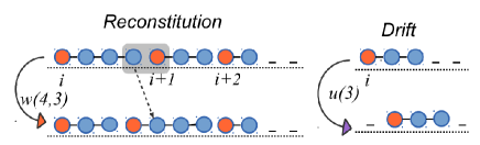
Figure 1: (Color online) Poly-dispersed $k$-mers in one dimension showing drift and reconstitution. Engine of the $k$-mers are marked as orange. The rate of drift $u(k)$ depends on the length of the corresponding $k$-mers. Reconstitution occurs only among consecutive immobile $k$-mers with a rate $w(k_{i},k_{i+1})$ which depends on their lengths. An additional constraint $w(k,k^{\prime})=0$ for $k<2$, conserves the number of $k$-mers in the system.

For completeness, we start with the model studied recently in daga_kmers . Let us consider $M$ number of $k$-mers on on a one dimensional periodic lattice of $L$ sites labeled by the index $i=1,2,...,L.$ The $k$-mers, each having different integer length, are also labeled sequentially as $m=1,2,\dots,M.$

A $k$-mer is a hard extended object which occupies $k$ consecutive sites on a lattice, and can be denoted by a string of $k$ consecutive $1$s (here represented by $1^{k}$). Thus, every configuration of the system can be represented by a binary sequence with each site $i$ carrying a variable $s_{i}=1$ or $0$ denoting respectively whether the lattice site is occupied by a $k$-mer or not. The total number of vacancies ($0$s) in the system is $N$ and thus, the total length of the $k$-mers is $K=\sum_{m=1}^{M}k_{m}=L-N$ (total number of $1$s). We define the free volume (or void density) as $\rho_{0}=N/L$ and the $k$-mer number density as $\rho=\frac{M}{L}$. Thus the packing fraction of the lattice (fraction of volume occupied by the $k$-mers) is $\eta=1-\rho_{0}=K/L.$

We consider directed diffusion of $k$-mers; a $k$-mer of size $k_{m}$ moves to its right with rate $u(k_{m}),$

$$k_{m}0\xrightarrow{u(k_{m})}0k_{m}~{}~{}\equiv~{}~{}1^{k_{m}}0\xrightarrow{u(k_{m})}01^{k_{m}}.$$ (1)

Along with this, reconstitution occurs among neighboring $k$-mers where one of the $k$-mers may release a single unit (or monomer) which instantly joins the other $k$-mer (see Fig. 1). Note that, reconstitution dynamics acts only at the interface of immobile $k$-mers which are expected to remain in contact for long,

$$(k_{m},~{}k_{m+1})\xrightleftharpoons[w(k_{m+1}+1,k_{m}-1)]{\,w(k_{m},k_{m+1})\,}(k_{m}-1,k_{m+1}+1).$$ (2)

The reconstitution rate $w(k_{m},k_{m+1})$ depends on the size of the participating $k$-mers and constrained by a condition $w(1,y)=0,$ which prohibits merging of $k$-mers and maintains the conservation of $k$-mer density $\rho.$ It is evident that Eqs. (1) and (2) also conserve $\rho_{0}.$

The dynamics of the model can be mapped exactly to a two-species generalization of misanthrope process (TMAP) footnote_TMAP by considering each $k$-mer as a box containing ${\kappa}=k-1$ particles of one kind ($k$-particles) and the number of consecutive vacancies (say $n$) in front of the $k$-mer as the number of particles of other type ($0$-particles). Thus, in TMAP, we have $M$ boxes containing $\tilde{K}=K-M$ number of $k$-particles and $N$ number of $0$-particles.

From a box $m$ containing $(n_{m},{\kappa}_{m})$ number of $0$- and $k$-particles respectively, the particles hop to one of the the neighboring boxes $m^{\prime}=m\pm 1$ having $(n_{m^{\prime}},{\kappa}_{m^{\prime}})$ particles with rates $u_{0}$ and $u_{k}$ (respectively for $0$- and $k$-particles),

$$u_{0}({\kappa}_{m})=u({\kappa}_{m}+1)\delta_{m^{\prime},m-1}$$ (3)

$$u_{k}({\kappa}_{m},{\kappa}_{m^{\prime}})=w({\kappa}_{m}+1,{\kappa}_{m^{\prime}}+1)\delta_{n_{m},0}\delta_{n_{m^{\prime}},0}.$$ (4)

The $\delta$-function in the first equation forces $0$-particles to move towards left (same as $k$-mers moving to the right neighbor on the lattice) and those in the last equation take care of the restrictions that reconstitution (or exchange of $k$-particles) occurs among boxes $m$ and $m^{\prime}$ only when they are devoid of $0$-particles (equivalently, when $k$-mers are immobile).

It is well known that misanthrope processes enjoy the luxury of factorized steady state EvansBeyondZRP for hop rates satisfying certain specific conditions. It is straight forward to derive similar conditions on hop rates of TMAP so that its steady state has a factorized form,

$$P({{\kappa}_{i},n_{i}})=\frac{1}{Q_{\tilde{K},N}}\prod_{i=1}^{M}f({\kappa}_{i},n_{i})\delta\small{\left(\sum_{i}{\kappa}_{i}-\tilde{K}\right)\delta\left(\sum_{i}n_{i}-N\right)},$$ (5)

where the $\delta$ functions ensure conservation of $\tilde{K},N,$ the total number of particles of each species, and $Q_{\tilde{K},N}$ is the canonical partition function. When the reconstitution rate in $k$-mer model has a product form $w(k,k^{\prime})=w_{1}(k)w_{2}(k^{\prime}),$ the hop rate of $k$-particles in corresponding TMAP (see Eq. (4)) also takes a product form $u_{k}({\kappa},{\kappa}^{\prime})=w_{1}({\kappa})w_{2}({\kappa}^{\prime}).$ For this simple choice, the weight function is given by daga_kmers ,

$$f({\kappa},n)=\frac{1}{[u_{0}({\kappa})]^{n}}\prod_{{\kappa}^{\prime}=1}^{{\kappa}}\frac{w_{2}({\kappa}^{\prime}-1)}{w_{1}({\kappa}^{\prime})}.$$ (6)

Once the functional forms of $u(.),w_{1}(.),w_{2}(.)$ are specified, one can calculate the steady state properties of the TMAP exactly from the partition function in grand canonical ensemble (GCE) using two fugacities $x$ and $z$ for the conservation of $\tilde{K}$ and $N$ respectively,

$$Z(x,z)=\sum_{\tilde{K}=0}^{\infty}\sum_{N=0}^{\infty}Q_{\tilde{K},N}x^{\tilde{K}}z^{N}.$$ (7)

From this partition function, one can further calculate one-point functions of the $k$-mer models analytically. However, spatial correlation functions can not be calculated straightforwardly. This is because the site variables $s_{i}=1,0$ on the $k$-mer model, which represent whether the site is occupied by a $k$-mer or not, are not so simple functions of the occupation numbers $\{n_{i},{\kappa}_{i}\}$ of TMAP. We have,

$$s_{i}=1-\sum_{j=1}^{M}\theta(g_{j}-i)\theta(i+2+n_{j}-g_{j});g_{j}=\sum_{l=1}^{j}(1+n_{l}+{\kappa}_{l});$$ (8)

where $\theta(x)$ is the Heaviside theta function. Clearly obtaining spatial correlation functions $C(r)=\langle s_{i}s_{i+r}\rangle-\langle s_{i}\rangle^{2}$ would be difficult (though not impossible) from the TMAP correspondence. In the following, we provide a matrix formulation to obtain the steady state weight of any configuration of the $k$-mer model from a matrix string which uniquely represents that configuration.

II.1 Matrix product steady state

To calculate the spatial correlation functions explicitly and conveniently, in this section, we provide a matrix formulation similar to the one obtained earlier for exclusion processes having ZRP correspondence OZRP . In OZRP , the authors showed that steady states of one dimensional exclusion models having ZRP correspondence can be written in matrix product form -they also provided an infinite dimensional representation of the matrices that can always be obtained from the corresponding ZRP weights footnote3 . In this article we try to obtain the spatial correlation functions of a polydispersed systems in a similar way, i.e., by writing the steady state weight of configuration as the trace of a representative matrix string.

How many matrices do we need ? In ZRP, or its equivalent exclusion process, there was only one conserved quantity, which is the density or the packing fraction $\eta.$ Here, we have an additional and independent conserved quantity $\rho,$ the $k$-mer density. Thus along with matrices $D$ and $E$ which represent the occupation status of a site we need another matrix, say $A$, that would appear once for every $k$-mer so that the $k$-mer number density is fixed appropriately. It is convenient to assign this matrix $A$ to the left most site (or an engine) of a $k$-mer. In other words, every $k$-mer ($1^{k}$ on a lattice) is represented by $AD^{k-1}.$ In summary, in the matrix formulation, all occupied sites except the engine $(A)$, are represented by matrix $D$s, and the vacant sites are represented by $E$s. Now, the steady state weight of a configuration $\{n_{i},k_{i}\}$ can be expressed (using ${\kappa}_{i}=k_{i}-1$ in Eq. (5)) as

$$\prod_{i=1}^{M}f(k_{i}-1,n_{i})=Tr\left[\prod_{i=1}^{M}AD^{k_{i}-1}E^{n_{i}}\right].$$ (9)

We further assume that $A$ can be expressed as an outer product of two vectors $A=|\alpha\rangle\langle\beta|$; the vectors $|\alpha\rangle,$ $\langle\beta|$ and matrices $D$ and $E$ need to be determined from the dynamics. With this choice, Eq. (9) results in,

$$f(k,n)=\langle\beta|D^{k}E^{n}|\alpha\rangle.$$ (10)

This equation is generic as long as the steady state of the TMAP corresponding to a reconstituting $k$-mer model has a factorized steady state. Now, any representation of $A=|\alpha\rangle\langle\beta|,D,E$ that satisfy Eq. (10) can provide a matrix product steady state for the $k$-mer model. One must, however, remember that any arbitrary matrix string does not necessarily represent a configuration of the $k$-mer model. Since every block of vacant sites (string of $E$s) must end with a $k$-mer represented by $AD^{k-1},$ all valid matrix strings must be devoid of $ED.$ This brings in an additional constraint,

$$ED=0$$ (11)

which must be accounted for while searching a suitable matrix representation.

We now restrict ourselves to specific $k$-mer dynamics which leads to a factorized steady state, as in Eq. (5). For the $k$-mer with hop rate $u(k)$ and reconstitution rate $\omega(k,k^{\prime})=w_{1}(k)w_{2}(k^{\prime})$, the steady state is given by Eq. (6). A set of matrices $\{\tilde{A},\tilde{D},\tilde{E}\}$ that satisfy Eq. (10)

$$\langle\tilde{\beta}|\tilde{D}^{k}\tilde{E}^{n}|\tilde{\alpha}\rangle=\frac{1}{[u(k+1)]^{n}}\prod_{k^{\prime}=1}^{k}\frac{w_{2}(k^{\prime}-1)}{w_{1}(k^{\prime})}$$ (12)

is

$$|\tilde{\alpha}\rangle=\sum_{i=1}^{\infty}|i\rangle;\langle\tilde{\beta}|=\langle 1|;\tilde{D}=\sum_{i=1}^{\infty}\frac{w_{2}(i-1)}{w_{1}(i)}|i\rangle\langle i+1|$$ (13)

$$\tilde{E}=|1\rangle\langle 1|+\sum_{i=2}^{\infty}\frac{1}{u(i-1)}|i\rangle\langle i|\;\;\;\;\;\;\;\;\;\;\;\;\;\;\;\;\;\;$$ (14)

where $\{|i\rangle\}$ with $i=1,2\dots$ are standard basis vectors in infinite dimension. These matrices, however, do not satisfy Eq. (11). One option is to discard this representation and look for a new one that satisfy both Eqs. (11) and (10), which can be done in certain specific cases (see next section). But Eq. (14) is a general representation for $k$-mer models where $k$-mers drift with rate $u(k)$ and reconstitute with a rate having product form $w(k,k^{\prime})=w_{1}(k)w_{2}(k^{\prime})$. Thus it would be beneficial to hold on to these matrices $\{\tilde{A},\tilde{D},\tilde{E}\},$ and to construct a new representation using them, which satisfy both Eqs. (10) and (11). In this context, the following representation works:

$$|\alpha\rangle=|\tilde{\alpha}\rangle\otimes(|\tilde{1}\rangle+|\tilde{2}\rangle),~{}~{}\langle\beta|=\langle\tilde{\beta}|\otimes\langle\tilde{2}|,$$ (15)

$$D=\tilde{D}\otimes|\tilde{2}\rangle\langle\tilde{2}|,~{}~{}E=\tilde{E}\otimes(|\tilde{1}\rangle+|\tilde{2}\rangle)\langle\tilde{1}|.$$ (16)

Here, $\{|\tilde{1}\rangle,|\tilde{2}\rangle\}$ are the standard (and complete) basis vectors in $2$-dimension. More explicitly, we have,

$$\begin{array}[]{ccc}A=\left(\begin{array}[]{cc}0&\tilde{A}\\ 0&\tilde{A}\\ \end{array}\right),&D=\left(\begin{array}[]{cc}0&0\\ 0&\tilde{D}\\ \end{array}\right),&E=\left(\begin{array}[]{cc}\tilde{E}&0\\ \tilde{E}&0\\ \end{array}\right)\\ \end{array}.$$ (17)

This infinite dimensional representation provides a matrix product steady state for drifting and reconstituting $k$-mers in one dimension as long as the re-constitution rate has a product form. In the following, we illustrate a specific case where the representation is finite dimensional.

III Constant-rate reconstitution (CRR) model

In this section we study a specific example of reconstituting $k$-mer model and illustrate the matrix product formulation presented in previous section. Let us consider that the $k$-mers drift to their right neighbor with rate $u(k)=1+(v-1)\delta_{k,1},$ i.e., the monomers ($k=1$) move with rate $v$ whereas other $k$-mers move with unit rate. Let the re-constitution rate be a constant $\omega,$ independent of the size of the $k$-mers. In this constant-rate reconstitution (CRR) model matrices $\{\tilde{A},\tilde{D},\tilde{E}\},$ which satisfy only Eq. (10), have two dimensional representations,

$$\begin{array}[]{ccc}\tilde{A}=\left(\begin{array}[]{cc}1&0\\ 1&0\\ \end{array}\right),&\tilde{D}=\omega\left(\begin{array}[]{cc}0&1\\ 0&1\\ \end{array}\right),&\tilde{E}=\left(\begin{array}[]{cc}\frac{1}{v}&0\\ 0&1\\ \end{array}\right)\\ \end{array}.$$ (18)

However, since these matrices do not satisfy Eq. (11), we now construct new matrices $\{A,D,E\},$ using Eq. (16), or (17),

$$A=\sum_{i=1}^{4}|i\rangle\langle 3|,\>\>D=\omega\sum_{i=3}^{4}|i\rangle\langle 4|,\;\;\;\;\;$$ (19)

$$E=\sum_{i=1}^{2}(\frac{1}{v}|2i-1\rangle\langle 2i-1|+|2i\rangle\langle 2i|)$$ (20)

which are 4-dimensional, and represent respectively the engine of the $k$-mer, any other unit of the $k$-mer and the vacancies $0$s.

To calculate the correlation function and the densities, as usual, we start with the partition function in GCE, $Z=Tr[T^{L}]$ where the transfer matrix $T=A+xD+zE.$ The fugacities $z$ and $x$ together control the densities $\rho_{0}$ and $\rho_{d}=1-\rho-\rho_{0}$, representing density of $E$s and $D$s respectively. In fact, in this problem, the transfer matrix $T\equiv T(z,x\omega,v)$ does not depend independently on $x$ and $\omega$, rather depends on their product. Thus, any particular value of $\omega$ only redefines the fugacity $x\to x\omega$ and we can set $\omega=1$ without loss of generality. Now, the partition function in GCE :

$$Z(z,x)=Tr(T^{L})~{};~{}T=A+xD+zE=\left(\begin{array}[]{cc}z\tilde{E}&\tilde{A}\\ z\tilde{E}&x\tilde{D}+\tilde{A}\\ \end{array}\right).$$ (21)

The characteristic equation for the eigenvalue of $T$ is $\lambda f(\lambda)=0,$ with

$$f(\lambda) = xz(1-v-z)+\{v+z+x(1+v)\}z\lambda$$ (23)

$$~{}~{}~{}~{}-\{z+v(1+x+z)\}\lambda^{2}+v\lambda^{3}.$$

Thus one of the eigenvalues of $T$ is $0$ and other three, denoted by the largest eigenvalue $\lambda_{max}$, and $\lambda_{1,2}$, are roots of the cubic polynomial $f(\lambda).$ The partition function in GCE is then,

$$Z(z,x) = \lambda_{max}(z,x)^{L}+\lambda_{1}(z,x)^{L}+\lambda_{2}(z,x)^{L}$$ (24)

$$\simeq \lambda_{max}(z,x)^{L}$$ (25)

where in the last step we have taken the thermodynamic limit $L\to\infty.$ The conserved densities of the canonical ensemble are now,

$$\rho_{d}=x\frac{\partial}{\partial x}\ln\lambda_{max},\,\,\rho_{0}=z\frac{\partial}{\partial z}\ln\lambda_{max}.$$ (26)

This density fugacity relation specify the values of $(z,x)$ which uniquely correspond to a particular pair of conserved densities $(\rho_{0},\rho_{d}).$ Any other observable in GCE, which are functions of $(z,x),$ can be expressed in terms of the densities $(\rho_{0},\rho_{d})$ using (26). We must mention that densities can also be obtained as follows.

$$\rho_{d}=\langle d_{i}\rangle = x\frac{Tr[DT^{L-1}]}{Tr[T^{L}]}~{};~{}\rho_{0}=\langle e_{i}\rangle=z\frac{Tr[ET^{L-1}]}{Tr[T^{L}]};$$ (27)

$$\rho = \langle a_{i}\rangle=\frac{Tr[AT^{L-1}]}{Tr[T^{L}]}.$$ (28)

Here $e_{i},a_{i},d_{i}$ are site variables which are unity when the site $i$ is vacant, occupied by an engine, or by other units of a $k$-mer, respectively; otherwise, $e_{i},a_{i},d_{i}$ are $0.$ In the thermodynamic limit, these definitions of densities are equivalent to Eq. (26).

III.1 Correlation functions

Now, we proceed to calculate the two point correlation functions. The engine-engine correlation function is

$$C(r)=\langle a_{i}a_{i+r}\rangle-\langle a_{i}\rangle^{2}=\frac{Tr[AT^{r-1}AT^{L-r-1}]}{Tr[T^{L}]}-\rho^{2},$$ (29)

which, in the thermodynamic limit, can generically be expressed as

$$C(r)=p_{1}(z,x;v)\left(\frac{\lambda_{1}}{\lambda_{max}}\right)^{r}+p_{2}(z,x;v)\left(\frac{\lambda_{2}}{\lambda_{max}}\right)^{r},$$ (30)

where $p_{1}$ and $p_{2}$ are independent of $r.$ The behavior of the correlation functions depend on the nature of eigenvalues $\lambda_{1,2},$ which can be determined from the properties of the characteristic function $f(\lambda)$, in Eq. (23). When the eigenvalues $\lambda_{1,2}$ are real, ordered as $\lambda_{max}>|\lambda_{1}|>|\lambda_{2}|,$ the system has two length scales $|\ln\frac{|\lambda_{1,2}|}{\lambda_{max}}|^{-1}$ and the asymptotic form of the correlation function is dominated by the largest one, $\xi=|\ln\frac{|\lambda_{1}|}{\lambda_{max}}|^{-1}.$ Correspondingly, the correlation has a monotonic exponential decay

$$C(r)\simeq p_{1}(z,x;v)e^{-r/\xi}.$$ (31)

Also, in some parameter zone eigenvalues $\lambda_{1,2}$ may become complex. As they appear as complex conjugates we write $\lambda_{1,2}=\bar{\lambda}e^{\pm i\theta},$ with $\bar{\lambda}<\lambda_{max}.$ In this regime, $p_{1,2}$ defined in Eq. (30) must be complex conjugates $p_{1,2}=\bar{p}e^{\pm i\phi}$ so that the correlation function $C(r)$ is real. Consequently $C(r)$ shows a damped oscillation, with a generic functional form

$$C(r)=\bar{p}e^{-r/\xi}\cos(\theta r+\phi),$$ (32)

where $\xi^{-1}=|\ln\frac{\bar{\lambda}}{\lambda_{max}}|.$

It is interesting to note that a damped oscillation of the radial distribution function is a typical feature of a system in liquid phase, in contrast to the exponential decay of the same in the vapor phase. Naively one would think that such a change is a direct consequence of an underlying liquid -vapor phase transition. However, this is not the scenario in CRR model; possibility of a phase transition is ruled out here as the largest eigenvalue $\lambda_{max}$ is non-degenerate for any $x,v,z$ and the corresponding free energy $\ln\lambda_{max}$ would not be non-analytic anywhere. This phenomena, a macroscopic change in the nature of correlation function in absence of any phase transition, has been known for a while in literature, in different contexts, under the name of disorder points (or lines). In a broad sense, the disorder points separate the regions in parameter space showing qualitatively different pair correlation functions and were first introduced by Stephenson step_1 . For Ising chains with ferromagnetic nearest-neighbor and anti-ferromagnetic next-nearest-neighbor interaction, the spin-spin correlation function in the disordered paramagnetic phase $(T>T_{c})$ shows damped oscillations when $T$ is larger than $T_{D}$ (the disorder point) whereas it decays exponentially for $T_{c}<T<T_{D}$ step_2 . There are several other lattice spin models aspects_dl ; latticespin_dl that exhibit disorder lines. In context of fluids, a similar behavior has been observed in the decay of density profiles and the radial distribution functions - here the disorder lines which separate different regimes are conventionally termed as Fisher-Widom lines fisher ; evans . Recent studies also indicate existence of disorder lines in phenomenological models of QCD at finite temperature and density nishimura_2015 .

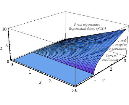
Figure 2: (Color online) Disorder surface separating regions where pair correlation function $C(r)$ decays exponentially (all three eigenvalues are real) from regions having damped oscillations (where the sub-dominant eigenvalues are complex).

In CRR model, there are three parameters - the monomer diffusion rate $v$ and the fugacities $x,z$ (or alternatively the densities $\rho,\eta$). Thus we have a two dimensional disorder surface that separates the regimes of exponential decay from that of the damped oscillatory correlation functions in the $(x,v,z)$ space. To identify the disorder surface we study the generic features of the characteristic function $\lambda f(\lambda)$ taking help of the Descartes’ sign rule. Since, all the parameters $x,v,z$ are positive, Descartes’ sign rule indicate that there is exactly one negative root when $z+v<1$ irrespective of the value of $x$. In this regime, the root other than $\lambda_{max}$ must be real, as complex roots are generated pairwise. In the region $z+v>1,$ we have at most three positive roots: one positive and two complex or all positive; the disorder surface that separates these regimes in $(x,v,z)$-space is shown in Fig. 2. In the region where the sub-dominant eigenvalues are ‘complex’, i.e., $\lambda_{1,2}=\bar{\lambda}e^{\pm i\theta}$ with $\bar{\lambda}<\lambda_{max},$ the correlation function exhibits damped oscillations.

The exact analytic expression of eigenvalues, densities and the two point correlation functions are rather lengthy. For the purpose of illustration, we provide the details in next section, for the CRR model only with $v=2$, which lead to both decaying and oscillating correlation functions in different density regimes separated by a disorder line.

III.2 CRR model with $v=2.$

In this sub-section we focus on the CRR model for a special case $v=2$. We have already set the reconstitution rate $\omega=1,$ thus the grand canonical partition function depends only on two parameters $z$ and $x$ which fix the densities $\rho_{0}$ and $\rho_{d}.$ The packing fraction, which is defined as the fraction of the lattice occupied by $k$-mers, is now $\eta=\rho+\rho_{d}=1-\rho_{0}.$ For $v=2,$ the eigenvalues are given by,

$$\{\lambda_{max},\lambda_{1},\lambda_{2}\}=\{g(1),g(\Omega),g(\Omega^{2})\}$$ (33)

where $g(y)=a+sy-\frac{p}{s}y^{2}$ and $\Omega=e^{i\pi/3}.$ The other parameters are, $a=3z+2x+2$ , $p=4(1+x)^{2}+3z(z-2x)$ and $q=8(1+x)^{3}+9z(z-2x)(x-2z)$ and $s^{3}=q+\frac{1}{2}\sqrt{4q^{2}-p^{3}}.$ The $k$-mer number density $\rho=1-\rho_{0}-\rho_{d}$ and the packing fraction $\eta=1-\rho_{0}$ are now calculated from Eq. (26),

$$\rho = \frac{(2\lambda_{max}-z)(\lambda_{max}-z)(\lambda_{max}-x)}{\lambda_{max}(6\lambda^{2}_{max}-2\lambda_{max}(3z+2x+2)+z^{2}+2z+3xz)}$$ (34)

$$\eta = \frac{\lambda_{max}(2\lambda_{max}-z)(\lambda_{max}-z)+xz}{\lambda_{max}(6\lambda^{2}_{max}-2\lambda_{max}(3z+2x+2)+z^{2}+2z+3xz)}.$$ (35)

In Fig. 3 we have plotted $\eta$ and $\rho$ as a function of $z,$ for different $x=0.01,0.1,1$ and $10$ respectively in(a) and (b).

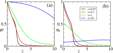
Figure 3: (Color online) Densities: (a) Packing fraction $\eta$ and (b) $k$-mer density $\rho$, as a function of $z$ for $x=0.01,0.1,1$ and $10.$

As expected, for $z=0,$ the packing fraction is $\eta=1,$ independent of the fugacity $x.$ On the other hand, in the limit $x\to 0,$ it appears that both $\eta$ and $\rho$ might become discontinuous at $z=2$ leading to a possibility of phase coexistence. In fact this seems to be the case for any $v>1$, and we discuss this possibility separately in the next section in details.

We now proceed to calculate the two point correlation functions, first the engine-engine correlation function $C(r)$ defined in Eq. (29). If we formally write the densities in Eq. (LABEL:eq:density_v2) as functions of $z,x$ and $\lambda_{max},$ as $\rho\equiv\hat{\rho}(z,x;\lambda_{max})$ and $\eta\equiv\hat{\eta}(z,x;\lambda_{max}),$ the engine-engine correlation function, calculated using Eq. (29), can be written as

$$C(r) = \langle a_{i}a_{i+r}\rangle-\rho^{2}=\rho\left[\hat{\rho}(z,x;\lambda_{1})\left(\frac{\lambda_{1}}{\lambda_{max}}\right)^{r}\right.$$ (38)

$$~{}~{}~{}~{}~{}+\left.\hat{\rho}(z,x;\lambda_{2})\left(\frac{\lambda_{2}}{\lambda_{max}}\right)^{r}\right].$$

Also, the density density correlation function $\langle s_{i}s_{i+r}\rangle-\eta^{2},$ takes a form similar to the right hand side of the above equation with $\rho\to\eta$ and $\hat{\rho}(.)\to\hat{\eta}(.).$ Clearly, $C(r)$ will exhibit damped oscillations when $\lambda_{1,2}=\bar{\lambda}e^{\pm i\theta}$ are complex. Whether such a regime, separated from the usual exponentially decay by a disorder line, exists for $v=2$, can be determined from the characteristic polynomial $\lambda f(\lambda).$ The discriminant of the $f(\lambda)$ vanishes for $x=z/2,$ which is the disorder line for $v=2$ (as shown in Fig. 4(a)); correspondingly the disorder line in $\eta$-$\rho$ plane (shown in Fig. 4(b)) is

$$\eta=\frac{\rho(\rho^{2}+3)}{(\rho+1)^{2}}$$ (39)

Thus, for $\eta>\frac{\rho(\rho^{2}+3)}{(\rho+1)^{2}}$ the correlation functions are expected to have damped oscillatory behavior whereas in the other regions the correlation functions must decay exponentially as a function of $r.$

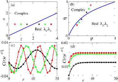
Figure 4: (Color online) Correlation functions: (a) For $v=2,$ complex roots appear for $x>z/2$, (b) the corresponding line in $\rho$-$\eta$ plane. (c) engine-engine correlation function $C(r)$ for $z=\frac{1}{2},1,\frac{3}{2}$ and (d) $z=\frac{5}{2},3,\frac{7}{2}.$ For (c) and (d), we use $x=1$, and the symbols used here for different $z$ are also marked in (a) and (b).

To illustrate this, we take $x=1,$ which indicates that the correlation functions must be oscillatory for any $z<2.$ In Fig. 4(c) and (d) we have plotted $C(r)e^{r/\xi}$ as a function of $r$ for $z=\frac{1}{2},1,\frac{3}{2}$ and $z=\frac{5}{2},3,\frac{7}{2}$ respectively. All these $(z,x)$ values are shown as symbols in Fig. 4(a). The corresponding densities are are shown in $\eta$-$\rho$ plane, marked as same symbols (in Fig. 4(b)). Clearly $C(r)e^{r/\xi}$ shows oscillations when $z<2,$ whereas it asymptotically approaches to a constant when $z>2.$ It appears that existence of disorder lines is a generic feature in extended systems; this may be a consequence of the hardcore restriction among $k$-mers which mimics a short range repulsion existing in model fluids.

We close this section with the following interesting remarks.

Remark 1: The four dimensional representation in CRR model leads to a transfer matrix $T$ with $Det[T]=0.$ This in turn means that one of the eigenvalues $\lambda=0,$ indicating that there might be a three dimensional representation which satisfy the matrix algebra Eqs. (10) and (11). We are able to find one such representation,

$$\begin{array}[]{ccc}A=\left(\begin{array}[]{ccc}1&0&1\\ 1&0&1\\ 0&0&0\\ \end{array}\right),&D=\left(\begin{array}[]{ccc}0&0&0\\ 0&0&0\\ 0&\omega&\omega\\ \end{array}\right),&E=\left(\begin{array}[]{ccc}\frac{1}{v}&0&0\\ 0&1&0\\ 0&0&0\\ \end{array}\right)\\ \end{array}$$ (40)

It is easy to check that $T=A+xD+zE$ gives the same characteristic polynomial $f(\lambda)$ as in Eq. (23).

Remark 2: For CRR model with $v=2,$ the line $x=z/2,$ which separates regions having damped oscillations from regions with exponentially decaying correlations is very special. On this line the engine-engine correlation function $C(r)$ vanishes, whereas the density-density correlation function remains finite. This can be verified from directly calculating the eigenvalues on this line, which are $\lambda_{max}=1+2x$ and $\lambda_{1}=x=\lambda_{2}.$ This makes the co-efficients $\hat{\rho}(z,x;\lambda_{1,2})=0$ in Eq. (38).

Remark 3: This formulation is inadequate to calculate spatial correlation functions of $k$-mer models when reconstitution is absent. Naively one may think, setting $\omega=0$ could work. But $\omega=0$ would impose a condition $\langle\beta|D^{k}E^{n}|\alpha\rangle=0$ for all $k,n$, which forces the weight of every configuration $Tr[...AD^{k}E^{n}A...]$ to vanish. In fact when $\omega=0,$ diffusion of $k$-mers (of different size) is the only dynamics on the lattice, which keeps the initial ordering of their size invariant. Now, the configuration space has infinitely many disconnected ordering-conserving sectors, and one must write partition sums separately for each sector.

Remark 4: In contrast to constant-rate reconstitution model, one may define a constant-rate diffusion model considering $u(k)=v,$ a constant. Now, let us consider a reconstitution rate $\omega(k,k^{\prime})=1+(\omega-1)\delta_{k,2}\delta_{k^{\prime},1},$ where dimers reconstitute with monomers at rate $\omega$ where as any other two $k$-mers reconstitute with unit rate. In this constant-rate diffusion model we have a simple two dimensional representation:

$$\begin{array}[]{ccc}A=\left(\begin{array}[]{cc}1&1\\ 0&0\\ \end{array}\right),&D=\left(\begin{array}[]{cc}0&0\\ w&1\\ \end{array}\right),&E=\left(\begin{array}[]{cc}\frac{1}{v}&0\\ 0&0\\ \end{array}\right)\\ \end{array}.$$ (41)

In a two dimensional representation both eigenvalues of $T=A+xD+zE$ (which is a positive matrix) are real and hence possibility of oscillatory feature in spatial correlation functions is ruled out.

III.3 Phase coexistence in CRR model in $x\to 0$ limit

In this section we investigate the CRR model in $x\to 0$ limit. We have seen in the previous section that for $v=2$, the $k$-mer density $\rho$ shows a sharp drop at $z=2.$ In fact this feature is quite generic for all $v>1.$ When the fugacity $x$ associated with $D$s approaches $0,$ we expect a microscopic number of $D$s in the system. In other words most $k$-mers are only monomers. Thus, the best case scenario that represents $x\to 0$ limit is a system with one single $D.$ Since this $D$ must be associated with an engine $A,$ we have exactly one dimer in the system which diffuses in the system with unit rate, and all other $k$ mers are monomers diffusing with rate $v.$ Thus, the dimer can be considered as a defect particle in the system. The re-constitution can occur only between this dimer and an adjacent monomer (when both are immobile) with rate $\omega=1.$ In this case, the reconstitution is equivalent to exchange of a monomer and a dimer.

Representing the single dimer as $2$ and the monomers as $1$s, and vacancies as $0$s, the dynamics of the system can be written as

$$10\xrightarrow{v}01~{}~{};~{}~{}20\xrightarrow{1}02~{}~{};~{}~{}211\xrightleftharpoons[1]{1}121.$$ (42)

Since this dynamics is only a special case of the CRR model, we can proceed with the $4\times 4$ representation given in Eq. (20). However, in this case there is a valid $2$-dimensional representation, because the weight of every configuration of the system can be written here as $Tr[AD\prod_{j=1}^{L-2}X_{i}],$ with $X_{i}$ being either $E$ or $A.$ Clearly, these matrix strings do not contain $ED$ and one need not bother about the constraint $ED=0$ in Eq. (11) and can work with the $2\times 2$ matrices $\{\tilde{A},\tilde{D},\tilde{E}\}.$ In other words, the dimer, monomer and vacancy are now represented by $D_{2}=\tilde{A}\tilde{D},$ $D_{1}=\tilde{A},$ and $\tilde{E}$ respectively. In GCE, the partition function is now

$$Z=Tr[D_{2}T^{L-2}];T=z\tilde{E}+D_{1}=\left(\begin{array}[]{cc}1+z/v&0\\ 1&z\\ \end{array}\right).$$ (43)

The eigenvalues of $T$ are $\{z,1+\frac{z}{v}\}$ and thus, for $v>1$ the maximum eigenvalue changes from being $\lambda_{max}=1+\frac{z}{v}$ to $\lambda_{max}=z$ at a critical fugacity $z_{c}=\frac{v}{v-1}.$ So, the partition function, in the thermodynamic system, $Z\sim\lambda_{max}^{L}$ is non-analytic at $z=z_{c}$ indicating a phase transition.

First we calculate the density profile, as seen from the defect, which can be expressed as

$$\rho(r)=\frac{Tr[D_{2}T^{r}D_{1}T^{L-3-r}]}{Tr[D_{2}T^{L-2}]}=\frac{\gamma}{z}\frac{z\gamma^{r}-z_{c}}{z\gamma^{L-2}-z_{c}}$$ (44)

where $r$ is distance from the defect site (or the dimer) and $\gamma=\frac{vz}{v+z}$ the ratio of eigenvalues. Thus, when $z<z_{c}$ or $\gamma<1,$ the profile $\rho(r)$ has a boundary layer in front of the defect site which extends over a length scale $1/|\ln\gamma|$ and for large $r\ll L,$ it saturates to a value $\rho_{s}=\gamma/z=v/(v+z).$ Thus for a thermodynamically large system, the bulk of the system has a density $v/(v+z),$ which is same as the expected monomer density in the thermodynamic limit,

$$\rho=1-z\frac{d}{dz}\ln\lambda_{max}=\frac{v}{v+z}.$$

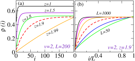
Figure 5: (Color online) (a) The density profile $\rho(i):$ (a) for $L=200,v=2$ and different $z=1,1.5,1.8,1.9,1.99.$ For small $z,$ $\rho(i)$ saturates to the macroscopic bulk density $v/(v+z).$ For large $z$ near $z_{c}$, such a saturation can be seen by increasing the system size $L$ - this is shown in (b). The profile for $z=1.9$ (marked as dashed line) as a function of $i/L$ shows saturation as $L$ increased.

In Fig. 5(a) we have plotted $\rho(r)$ for different $z$ considering $v=2$ (corresponding bulk densities are $\rho_{s}=2/(2+z).$ It is evident that for a small system (here $L=200$) the boundary layer invades into the bulk as $z$ approaches the critical value $z_{c}.$ However, for any $z\lessapprox z_{c},$ the boundary layer shrinks to $r=0$ in the thermodynamic limit $L\to\infty.$ This is shown in Fig. 5(b) for $z=1.9$ ( here $z_{c}=2$) and $L=50,100,200,400,700,1000.)$

The fugacity $z$ associated with the vacancies can tune the density of the monomers in the regime $z<z_{c},$ which corresponds to a density regime $\rho_{c}<\rho<1,$ where $\rho_{c}=1-1/v.$ In the canonical ensemble, if the conserved density is fixed at some value $\rho<\rho_{c},$ the system is expected to show phase coexistence. Since the allowed macroscopic densities are $\rho_{c}$ and $0,$ and the average density has to be $\rho$, the system would allow a local density $\rho_{c}$ in $\delta=\rho/\rho_{c}$ fraction of the lattice and keep $1-\delta$ fraction vacant.

The single dimer problem we discussed here is very similar to the single defect in totally asymmetric simple exclusion process (TASEP) studied earlier in Mallick1996 ; Derrida1999 . This TASEP model comprises of a single defect particle (denoted by $2$) and $L-1$ normal particles ($1$s) on a ring of size $L$, following a hopping dynamics,

$$10\xrightarrow{1}01~{}~{};~{}~{}20\xrightarrow{\alpha}02~{}~{};~{}~{}21\xrightarrow{\beta}12.$$ (45)

A special case of the model $\alpha=1=\beta$ Lebowitz corresponds to a scenario where the defect $2$ is a second-class particle which helps in locating the shocks, if any. The model defined by the above dynamics, can be solved using matrix product ansatz Mallick1996 ; evans_asep , but the matrices $\{E,D,A\}$ corresponding to $\{0,1,2\}$ have an infinite dimensional representation, closely related to the matrices $\{E,D\}$ in TASEP derrida_mpa . A novel feature that arises in this model is the phase coexistence - for $\beta<\rho<1-\alpha,$ the system shows a coexistence between a region of low-density $\beta$ in front of the defect, and a high-density $1-\alpha$ behind it. Thus a localized shock is formed at the site $j=\delta N,$ such that the conserved density $\rho=\beta\delta+(1-\alpha)(1-\delta).$ In the following, we compare the phase coexistence scenario of this model with the single dimer model studied here.

The dynamics of the single dimer model, Eq. (42), is equivalent to

$$10\xrightarrow{1}01~{}~{};~{}~{}20\xrightarrow{1/v}02~{}~{};~{}~{}211\xrightleftharpoons[1/v]{1/v}121.$$ (46)

However, in contrast to Eq. (45) there are two major differences in (46). Firstly the dimer occupies two lattice sites, whereas the defect particle $2$ in exclusion processes occupies only one lattice site - this difference is not crucial in the thermodynamic limit. Secondly, in comparison to the defect dynamics in Eq. (45), (i) the dimer can exchange with a monomer in both directions, and (ii) the exchange occurs only when the immediate right neighbor of the exchanging sites is occupied.

If we overlook these differences, the models are similar when $\alpha=1/v=\beta.$ Thus one may speculate that a phase coexistence may occur when $\frac{1}{v}<\rho<1-\frac{1}{v}.$ In reality, however, for dynamics (42), phase coexistence occurs when $0<\rho<\rho_{c}=1-\frac{1}{v}.$ This similarity is striking - particularly when the matrix representation for (45) is infinite dimensional whereas the same for (42) is much simpler, $2\times 2$ matrices.

IV Conclusion

In this article we provide a general formulation to write the steady state weights of reconstituting $k$-mer models in matrix product form. In the matrix formulation, we represent a vacancy by a matrix $E$, the engine of a $k$-mer (leading monomer unit from the left) by $A$ and rest of the monomer units by $D$s. In these models, the $k$-mers, which are extended objects of different sizes, move to neighboring vacant sites with a rate that depends on their size. Reconstitution can occur among a pair of $k$-mers, when they are in contact, with a rate that depends on size of participating objects. Reconstitution usually means transfer of a monomer from one $k$-mer to the other one; we restrict such a transfer if length of the $k$-mer transferring a monomer, is unity. This keeps the number of $k$-mers conserved. These models can not be solved exactly for any arbitrary diffusion and reconstitution rates. Some of them can be solved, under quite general conditions, using a mapping of $k$-mer models to a two species misanthrope process. These exactly solvable models, though simple, capture the different phases of the system and possible transitions among them daga_kmers ; Daga2016 quite well. However, calculating spatial correlation functions through this mapping is usually a formidable task, as the mapping does not keep track of the site-indices and the notion of distance. Thus, rewriting the steady state weights in terms of a matrix product form is greatly useful.

If $k$-mers are mono-dispersed, i.e., each one has a fixed length $k$, the matrix product form is relatively simple gupta_kmer . This is because, the density of $k$-mers $\rho$ dictates the packing fraction $\eta=\rho k$, and one can get away with two matrices $D$ and $E$ representing whether the site is occupied or not. The fact, poly-dispersed systems studied here have two independent conserved quantities $\rho$ and $\eta$, brings in additional complications. First, to write the steady state in matrix product form, we need an additional matrix $A$ (along with $D,E$) to identify the $k$-mers and to keep track of the conserved $k$-mer number. Next, additional care must be taken to ensure that every block of vacancies must end with $A$- in other words all configurations must be devoid of $ED.$

In summary, the reconstituting $k$-mer models for which the steady state weights can be obtained exactly through a two species misanthrope process, we device a matrix formulation to calculate spatial correlation functions explicitly. The required matrix algebra, and a generic representation that satisfies this algebra are also provided. Specifically, we demonstrate the formulation for the constant-rate reconstitution (CRR) model where reconstitution occurs with a constant rate $\omega,$ and all $k$-mers except the monomer, move to its right neighbour (if vacant) with unit rate; the rate for monomers is $v\neq 1.$ The two point spatial correlation functions of CRR model show interesting behavior when $k$-mer density $\rho$ and packing fraction $\eta$ are tuned. In some density regime the spatial correlation functions show damped oscillation whereas in other regimes they decay exponentially. The boundary that separates these regimes in $\rho$-$\eta$ plane, conventionally known as the disorder line, is calculated analytically.

A special limit $\eta\to\rho$ of the CRR model is best represented by a system of monomers and a single dimer. The reconstitution process in this single dimer model is equivalent to exchange of a monomer with the dimer, when in contact. Effectively, the dimer behaves like a defect in the system and exhibits a phase coexistence, similar to the one observed in asymmetric exclusion processes with a single defect. We must mention that, though both models capture the phase separation scenario, the single dimer model is represented by a set of simpler $2\times 2$ matrices in contrast to the infinite dimensional representation in exclusion processes with a defect.

In all through this article we have considered directed diffusion of $k$-mers. This provides a natural interpretation that reconstitution occurs among immobile $k$-mers. However, the steady state and thus physical properties of the model are invariant if we use, a symmetric diffusion of $k$-mers, and a reconstitution process that does not allow two particles of different species (in corresponding two species misanthrope process) to move out of a box simultaneously.

In this article we provide matrix product steady states for a class of $k$- mer models, by mapping them to a two species misanthrope process. In fact any two species misanthrope process can be mapped to a lattice containing extended objects - the steady state of such systems can always be be written in matrix product form. We believe that the matrix formulation developed here can be useful, in general, to explore spatial correlation functions in extended systems in one dimension.

References

- (1) B. Schmittmann and R. K. P. Zia, Statistical Mechanics of Driven Diffusive Systems, Vol. 17 of Phase Transitions and Critical Phenomena, edited by C. Domb, J. L. Lebowitz (Academic Press, 1995).
- (2) Nonequilibrium Phase Transitions in Lattice Models, J. Marro and R. Dickman, Cambridge University Press, 1999.
- (3) J. Krug, Phys. Rev. Lett. 67, 1882 (1991).
- (4) B. Derrida, M. R. Evans, V. Hakim and V. Pasquier, J. Phys. A 26, 1493 (1993).
- (5) for review, see, R. A. Blythe and M. R. Evans, J. Phys. A 40, R333 (2007).
- (6) M. R. Evans, D. P. Foster, C. Godréche, and D. Mukamel, Phys. Rev. Lett. 74, 208 (1995).
- (7) Y. Kafri, E. Levine, D. Mukamel, G. M. Schütz and J. Török Phys. Rev. Lett. 89 035702 (2002).
- (8) for review, see, M. R. Evans and T. Hanney, J. Phys. A 38 R195-R240 (2005).
- (9) J. S. Hager, J. Krug, V. Popkov, G. M. Schütz Phys. Rev. E 63, 056110 (2001).
- (10) V. Popkov, A. Rákos, R. D. Willmann, A. B. Kolomeisky, and G. M. Schütz, Phys. Rev. E 67, 066117(2003); Yu-Q. Wang, R. Jiang, A. B. Kolomeisky, and M-B. Hu, Sc. Reports 4, 5459 (2014).
- (11) S. Katz, J. L. Lebowitz and H. Spohn, Phys. Rev. B 28, 1655 (1983); S. Katz, J.L. Lebowitz and H. Spohn, J. Stat. Phys. 34, 497-537 (1984).
- (12) C. T. MacDonald, J. H. Gibbs, and A. C. Pipkin, Biopolymers 6, 11 (1968); C. T. MacDonald and J. H. Gibbs, Biopolymers 7, 707 (1969).
- (13) L. B. Shaw, R. K. P. Zia and K. H. Lee, Phys. Rev. E 68 021910 (2003).
- (14) D. Chowdhury, L. Santen, and A. Schadschneider, Phys. Rep. 329, 199(2000).
- (15) T. Chou and D. Lohse, Phys. Rev. Lett. 82 3552 (1999).
- (16) Y. Aghababaie, G. I. Menon, and M. Plischke, Phys. Rev. E59, 2578 (1999); A. Parmeggiani, T. Franosch and E. Frey, Phys. Rev. Lett. 90 086601 (2003).
- (17) M. R. Evans, C. Godrëche, D. P. Foster, and D. Mukamel, J. Stat. Phys. 80, 69 (1995); F. C. Alcaraz, S. Dasmahaptra, and V. Rittenberg , J. Phys. A: Math. Gen. 31 845 (1998); U. Basu, P. K. Mohanty, Phys. Rev. E 82, 041117 (2010).
- (18) M. R. Evans, Y. Kafri, H. M. Koduvely, and D. Mukamel, Phys. Rev. Lett. 80, 425 (1998); M. R. Evans, Y. Kafri, H. M. Koduvely, and D. Mukamel, Phys. Rev. E 58, 2764 (1998).
- (19) Y. Kafri, E. Levine, D. Mukamel, G.M. Schütz, and R. D. W. Willmann, Phys. Rev. E 68, 035101 (2003); M. R. Evans, E. Levine, P. K. Mohanty, and D. Mukamel, Eur. Phys. J. B 41, 223(2004).
- (20) L. Tonks, Phys. Rev. 50, 955 (1936)
- (21) T. Sasamoto and M. Wadati, J. Phys. A: Math. Gen. 31, 6057 (1998).
- (22) L. B. Shaw, R. K. P. Zia, and K. H. Lee, Phys. Rev. E 68, 021910 (2003).
- (23) G. Schönherr and G. M. Schütz, J. Phys. A: Math. Gen. 37, 8215 (2004).
- (24) L. B. Shaw, A. B. Kolomeisky, and K. H. Lee, J. Phys.A: Math. Gen. 37, 2105 (2004).
- (25) L. B. Shaw, J. P. Sethna, and K. H. Lee, Phys. Rev. E 70, 021901 (2004).
- (26) J. J. Dong, B. Schmittmann, and R. K. P. Zia, Phys. Rev. E 76, 051113 (2007).
- (27) B. Daga and P. K. Mohanty, JSTAT P04004 (2015).
- (28) G. I. Menon, M. Barma, and D. Dhar, J. Stat. Phys. 86, 1237 (1997).
- (29) S. Gupta, M. Barma, U. Basu and P. K. Mohanty, Phys. Rev. E 84 041102 (2011).
- (30) Z. W. Salsburg, R. W. Zwanzig and J. G. Kirkwood, J. Chem. Phys. 21, 1098 (1953).
- (31) F. C. Alcaraz and R. Z. Bariev, Phys. Rev. E 60, 79 (1999).
- (32) D. Dhar, Physica A 315 5 (2002).
- (33) M. Barma, M. D. Grynberg and R. B. Stinchcombe, J. Phys.: Cond. Mat. 19, 065112 (2007).
- (34) M. D. Grynberg, Phys. Rev. E 84, 061145 (2011).
- (35) In misanthrope process EvansBeyondZRP , a particle hops from a site to one of its neigbours with a rate that depends on the number of particles of both the departure and the arrival sites. A two species misanthrope process (TMAP) is a generalization, where the hop rate of each species depends on occupation number of both species in departure and arrival sites.
- (36) M. R. Evans and B. Waclaw, J. Phys. A: Math. and Theo. 47, 095001 (2014).
- (37) U. Basu and P. K. Mohanty, JSTAT L03006 (2010).
- (38) Additional care must be taken at the transition point Kavita_Arvind , where ensemble equivalence is in question.
- (39) Priyanka, A. Ayyer, and K. Jain, Phys. Rev. E 90, 062104 (2014).
- (40) J. Stephenson, Can. J. Phys. 48 1724 (1970).
- (41) J. Stephenson, Phys. Rev. B 1, 4405 (1970); ibid, J. Math. Phys. 11, 420 (1970); ibid, J. Appl. Phys. 42, 1278 (1971).
- (42) T. Garel, J. C. Niel, H. Orland, and M. Schick, J. Phys. A Math. Gen. 24, 1245 (1991).
- (43) M. T. Batchelor and J. M. J. Van Leeuwen, Physica A 154, 365 (1989).
- (44) M. Fisher and B. Widom, J. Chem. Phys. 50, 3756 (1969).
- (45) R. Evans , J. R. Henderson , D. C. Hoyle , A. O. Parry and Z. A. Sabeur, Mol. Phys. 80, 755 (1993).
- (46) H. Nishimura, M.C. Ogilvie and K. Pangeni, Phys. Rev. D 91, 054004 (2015).
- (47) K. Mallick, J. Phys. A: Math. Gen. 29 5375 (1996).
- (48) B. Derrida and M. R. Evans, J. Phys. A: Math. Gen. 32, 4833 (1999).
- (49) B. Derrida, S. A. Janowsky, J. L. Lebowitz, and E. R. Speer, J. Stat. Phys. 73 813 (1993).
- (50) B. Daga, arXiv:1604.05477