Markov State Modeling of Sliding Friction

Abstract

Markov State Modeling has recently emerged as a key technique for analyzing rare events in thermal equilibrium molecular simulations and finding metastable states. Here we export this technique to the study of friction, where strongly non-equilibrium events are induced by an external force. The approach is benchmarked on the well-studied Frenkel-Kontorova model, where we demonstrate the unprejudiced identification of the minimal basis microscopic states necessary for describing sliding, stick-slip and dissipation. The steps necessary for the application to realistic frictional systems are highlighted.

Despite the relevance of friction between solids from the macroscale to the nanoscale, its physical description still needs theoretical basis and understanding. Even the simplest, classical atomistic sliding problem has too many degrees of freedom, and there is so far no method for the unprejudiced identification of a few dynamical collective variables suitable for a mesoscopic description of fundamental sliding events such as stick-slip Gnecco and Meyer (2015). In the field of equilibrium biomolecular simulations, where computational scientists often meet similar problems, powerful tools have been developed in the last decade, aimed at identifying the relevant metastable conformations, the reactions paths, and the rates associated to transition events between them. In particular, Markov State Models Schwantes et al. (2014); Noé and Nüske (2013); Bowman et al. (2014); Schütte and Sarich (2015) (MSMs) have emerged as a key technique, with clear theoretical foundations and great flexibility. In that approach, the dynamical trajectory in phase space of a large collection of molecular entities is projected onto a much smaller space defined by a discrete set of states that are deemed typical, and the dynamics is reduced to Markovian jumps between these states. In most cases so far MSMs were applied to systems at equilibrium, where a stationary measure is defined and the Markov description is natural. In the physics of friction we deal with strongly nonequilibrium dynamics, even in steady state sliding. Application of MSMs to nonequilibrium problems is still in its infancy, with apparently only one instance, related to periodic driving Wang and Schütte (2015).

Here we show how the MSM framework can be extended to the study of nanofriction dynamics. To demonstrate that concretely, we choose one of the simplest tribological models, the one-dimensional Frenkel-Kontorova (FK) model Frenkel and T A Kontorova (1938) in its atomic stick-slip regime Braun and Kivshar (1998); Paliy et al. (1997). The MSM construction leads to the identification of a handful of natural variables which describe the steady-state dynamics of friction in this model.

Starting from the set of configurations obtained with a simulation of steady-state sliding, the first step of the construction is to define a metric in the high dimensional phase space of the original model, then used to identify a small number of microstates, by means of a recently proposed clustering algorithm Rodriguez and Laio (2014). The statistics of transitions between configurations is shown to be compatible with a description as a Markov process between the microstates. The highest eigenvectors of the transfer operator provide a novel characterization of the slowest modes of frictional motion. The space of microstates can be further coarse-grained into a few macrostates using standard coarse-graining methods,  Deuflhard and Weber (2005); Weber and Kube (2005) finally yielding a compact MSM description. In it, the time evolution of observables such as frictional work and displacement still reproduces the main features of the original frictional dynamics. The states of this Markov process reveal the definition of the collective variables describing friction, which for the simple FK model are the kink-antikink populations, but should be naturally found also in out of equilibrium sliding systems of higher and generic complexity.

The transfer operator and matrix — Our analysis is based on the Transfer Operator (TO) formalism Bowman et al. (2014). Denote by $\Pi^{\tau}(X\rightarrow X^{\prime})$ the probability to go from a configuration $X^{t}=X$ at time $t$ to $X^{t+\tau}=X^{\prime}$ at time $t+\tau$. While $\Pi^{\tau}$ is a continuous process and would take infinite time to sample, we build a coarse-grained TO by partitioning the configuration space into microstates (ensembles of similar configurations) $\{c_{\alpha},\alpha=1,\dots,n_{c}\}$. Between these microstates the restricted TO is a finite $n_{c}\times n_{c}$ Transfer Matrix (TM) with the generic element $\Pi_{\alpha\beta}^{\tau}=\int_{X\in c_{\alpha}}\int_{X^{\prime}\in c_{\beta}}{\rm d}X{\rm d}X^{\prime}P(X)\Pi^{\tau}(X\rightarrow X^{\prime})$, the probability to go from $c_{\alpha}$ to $c_{\beta}$ in time $\tau$. This TM contains less detail than the full $\Pi_{\alpha\beta}^{\tau}$. Being simpler, it is more informative, and can be sampled with satisfactory statistics in much less time. Of course $\Pi_{\alpha\beta}^{\tau}$ also depends on the lagtime $\tau$, but there are techniques to control the error related to the choice of this parameter (see SI 1.1). Given the TM, we calculate its eigenvalues $\{\lambda_{i}\}$ and left eigenvectors $\{\vec{\chi}_{i}\}$. Because we are not in equilibrium, detailed balance does not hold, the TM is not symmetric and the eigenvalues are not necessarily real. However, they still satisfy $\left|\lambda_{i}\right|\leq 1$ by the Perron-Frobenius theorem. The largest (modulus-wise) eigenvalue is exactly $1$, and if the evolution is ergodic there is only one such eigenvalue. The eigenvector $\vec{\chi}_{1}$ represents the invariant, steady state distribution, endowed with nonzero sliding current. The eigenvectors $\vec{\chi}_{i}$ with $\left|\lambda_{i}\right|\simeq 1$ form the so-called Perron Cluster Deuflhard and Weber (2005). They characterize the long-lived excitations of the steady state, which decay with long characteristic times $\tau_{i}=-\tau/\ln\left|\lambda_{i}\right|\gg\tau$, while oscillating with period $\tau/\arctan({\rm Im}\lambda_{i}/{\rm Re}\lambda_{i})$.

The Frenkel-Kontorova model — The one-dimensional FK model, Fig. 1(a), our test case, consists of a chain of particles dragged over a sinusoidal potential $V(x)=A\cos(2\pi x/a)$. Nearest neighbor springs of stiffness $k$ link $L$ classical particles of mass $m$ and positions $x_{i}$ whose spacing $a$ is commensurate with the potential. Each particles is dragged by a spring of constant $\kappa$ moving with constant velocity $v_{{\rm ext}}$. Particle motion obeys an overdamped Langevin dynamics (large damping $\gamma$), in a bath of inverse temperature $\beta=1/k_{B}T$:

$$\begin{array}[]{rcl}x_{l}^{t+dt}&=&\displaystyle x_{l}^{t}+\left(\frac{2\pi A}{\gamma ma}\sin\left(\frac{2\pi x_{l}^{t}}{a}\right)+\frac{\kappa}{\gamma m}(v_{\rm ext}t-x_{l}^{t})+\right.\\ &&\displaystyle\left.-\frac{k}{\gamma m}(2x_{l}^{t}-x_{l-1}^{t}-x_{l+1}^{t})\right)dt+\sqrt{\frac{2dt}{\gamma m\beta}}f^{t},\end{array}$$ (1)

where $f^{t}$ is an uncorrelated Gaussian distribution and $dt$ is the elementary time step (here $dt=10^{-2}$). Our input is the steady-state trajectory of the chain, obtained by integrating these equations, mostly for the simplest case of $L=10$ (but also $L=15,20$) and a sufficient duration of $10^{6}$ time units.

As is well known Braun and Kivshar (1998), in a wide range of parameters the chain sliding alternates long sticking periods during which particles are close to their respective potential minima with fast slips during which one or more lattice spacings are gained. This kind of atomic stick-slip motion is well established for, e.g., the sliding of an Atomic Force Microscope tip on a crystal surface Vanossi et al. (2013). The slip event involves the formation of kink/antikink defects (large deviations of the interparticle distance from the equilibrium value) that propagate along the chain and enable the global movement. A sample of steady-state sliding evolution can be seen in Fig. 1(b), showing the finer details of each particle’s motion for a few slip events.

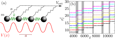
Figure 1: (a) Schematic of the FK system. (b) Sample of steady-state motion of $L=10$ particles with parameters $k=0.04$, $A=0.1$, $a=1.5$, $m=1$, $\gamma=1$, $\beta=500$, $\kappa=0.01$, $v_{{\rm ext}}=0.001$. The white and grey backgrounds represent stick and slip time domains respectively.

With this trajectory in the $L$-particle phase space the building of our Markov State Model (MSM) (see e.g. Schütte and Sarich (2015)) involves three steps : choice of a metric, clustering into microstates, and construction of macrostates and their reduced TM dynamics.

Metric — The phase space explored under steady sliding grows linearly with time and is thus generally very poorly sampled. Internal variables are free of this problem; a viable metric in phase space can therefore include e.g., the bond lengths $b_{l}^{t}=(x_{l+1}^{t}-x_{l}^{t}-a)/a$. On the other hand the inclusion of growing degrees of freedom like the position of the center of mass (CM): $x_{\rm CM}^{t}=\frac{1}{Na}\sum_{l=1}^{L}x_{l}^{t}$ cannot be implemented without caution. Sampling can be improved if distinct parts of the steady-state evolution can be considered as equivalent. Ideally, we could consider a portion of the evolution long enough that all relevant events (here, frictional slips) have occurred, then set “absorbing” boundary conditions for any such transition from and to the outside of this range, then averaging over many such equivalent stretches. In the alternative approach which we adopt here, we substitute the absorbing conditions with artificially periodic boundary conditions, a choice which provides a more compelling picture of steady-state sliding, and where the error involved in the transition rates can be reduced at will by extending the portion size. In the FK system, we exploit the substrate periodicity and $x_{\rm CM}$ is taken modulo $na$ for a chosen integer $n>1$. Under slow driving, $n=2$ is sufficient for a correct description of slips by $a$ (atomic slip), and states divide into even and odd $x_{\rm CM}$. If slips of $2a$, $3a$ or more became more frequent, we would simply choose a larger $n$. The full set of steady state sliding data is used to generate many independent configurations, all treated in the same manner. Summing up, the metric we adopt defines the distance between configurations at times $s$ and $t$ as

$$d_{st}=\left[(x^{s}_{\rm CM}-x^{t}_{\rm CM})_{\text{mod }2}\right]^{2}+\sum_{l=1}^{L-1}\left(b^{s}_{l}-b^{t}_{l}\right)^{2}.$$ (2)

Microstates — In the second step, configurations whose relative distance is small are collected together, in $n_{c}$ microstates. Microstates are built by the Density Peak algorithm Rodriguez and Laio (2014), which efficiently traces them as maxima of the probability density in phase space. Given a distance $d_{st}$ between two configurations $X^{s}$ and $X^{t}$ we estimate the local density $\rho^{s}$ in $X^{s}$ by counting the number of configurations within a cutoff $d_{c}$, $\rho^{s}=\sum_{t}\theta(d_{c}-d_{st})$ where $\theta$ is the step function. One then computes the distance $\delta^{s}$ between $X^{s}$ and the closest configuration of higher density, $\delta^{s}=\min_{\rho^{t}>\rho^{s}}d_{st}$ and identifies the microstate centers as the $n_{c}$ points with the highest product $\delta^{s}\rho^{s}$. All remaining points are assigned to the microstate of highest local density. This clustering technique allows finding microstates of variable volume in phase space, and well-defined cluster centers (configurations often visited), both desirable features in building a MSM. The next step is the dynamics between microstates which we describe in the FK model.

We use samples of $N=10^{5}$ configurations (separated by the lagtime $\tau$) and cluster them using the metric (II.1). The optimal lagtime $\tau$ is determined by studying the evolution of the spectrum of the clustered TM with $\tau$ (see SI sec. 1). We find a plateau around the value $\tau=10=1000dt$, showing that the dynamics is Markovian in this range. With $\tau=10$, the algorithm detects a PC of $n_{c}\simeq 100$ microstates. Besides $\lambda_{1}=1$, the spectrum of the $n_{c}\times n_{c}$ TM is characterized by a second eigenvalue $\lambda_{2}$ (see Fig. 2), corresponding to a relaxation time of $\simeq 600$, separated by a gap from other eigenvalues with shorter relaxation times. The significance of the eigenmodes $\chi_{i}$ is clarified by considering the probability distribution $P\left(O,t\right)$ of an observable $O$ at time $t$, starting from a system prepared in the mixed state $P^{0}_{\alpha}$ (probability vector to be in $c_{\alpha}$ at $t=0$). We have:

$$P\left(O,t\right)=P^{\rm ss}\left(O\right)+\sum_{i>1}f_{i}g_{i}\left(O\right)e^{-t/\tau_{i}},$$ (3)

where $f_{i}=\sum_{\alpha}\chi_{i}^{\alpha}P^{0}_{\alpha}/P^{\rm ss}_{\alpha}$ accounts for the initial condition and

$$g_{i}\left(O\right)=\sum_{\alpha}\chi_{i}^{\alpha}P(O|\alpha),$$ (4)

where $P(O|\alpha)$ is the probability distribution of $O$ in microstate $\alpha$, $P^{\rm ss}(O)=g_{1}(O)$ the steady state distribution of $O$, and $P_{\alpha}^{\rm ss}$ the steady state probability to visit microstate $\alpha$. The $g_{i}(O)$ for $i>1$ represent “perturbations” of $P^{\rm ss}(O)$, each decaying within the lifetime $\tau_{i}$.

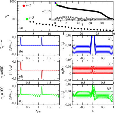
Figure 2: (a) Characteristic timescales and eigenvalues (in the inset, imaginary part in white) of the TM (averaged over 10 realizations with $N=10^{5}$ each). (b),(d),(f) Probability distribution $g_{1}(x_{\rm CM})$ and perturbations $g_{i}(x_{\rm CM})$ of the center of mass position $x_{\rm CM}$ for the first $3$ eigenvectors of the TM. (c),(e),(g) Probability distribution $g_{1}(b_{l})$ and perturbations $g_{i}(b_{l})$ of each bond $b_{l}$ for the first $3$ eigenvectors of the TM (successive bonds $b_{l}$ are spaced vertically of $0.005$ each, for clarity).

In Fig. 2(b)(d)(f) we plot $g_{i}(x_{\rm CM})$: the steady state $\chi_{1}$ consists of one large peak per period plus $9$ smaller peaks, corresponding to the relaxed chain state and defect combinations, respectively. The second eigenvector $\chi_{2}$ presents exactly the same features, except for a factor $-1$ in the second period: in the combinations $\chi_{1}\pm\chi_{2}$ the chain CM sticks either in an odd or even position. The second eigenvector is thus representative of the main advancing motion of the chain, namely the slip. Indeed $t_{2}=-\tau/\log(\lambda_{2})\simeq 600$ is about half the sticking time (see Fig. 1). In Fig. 2(c)(e)(g) we plot $g_{i}$ ($i=1,2,3$) for the bond lengths $b_{l}$. In the steady state $\chi_{1}$ each bond length has high peaks around its value at rest $(0)$ and smaller ones around $b\simeq\pm 0.9$, reflecting the infrequent appearance of excitations, that are kinks or antikinks. The second mode $\chi_{2}$ shows a flat distribution, since all the difference with $\chi_{1}$ lies in the CM degree of freedom, $x_{\rm CM}$. In fact $\chi_{3}$ displays small central peaks and more pronounced lateral ones, corresponding to the creation (destruction for negative peaks) of a kink or antikink (depending on the sign of $b_{l}$) Braun and Kivshar (1998), excitations with shorter lifetimes. Indeed, $t_{3}\simeq 100$ is comparable to the half-lifetime of kinks and anti-kinks. Furthermore, we can see how the peaks tend to be positive for the first $b_{l}$’s and negative for the last ones, implying that the chain tends to be elongated in its head and compressed in its tail. This shows that kink-antikink pairs are more likely to be formed in the center of the chain, intrinsic to the slip mechanism for this system. At this stage one can already identify the kink and antikink populations as the relevant collective variables of sliding, together with $x_{\rm CM}$. While these gross features of a commensurate FK stick-slip are therefore already contained in the first few long-lived microstates with largest eigenvalues, a more accurate description must involve a quantitative analysis of the whole Perron cluster.

Macrostates — In the third and final step, the $n_{c}$ microstates are coarse-grained and grouped into macrostates. A well established approach for that is the (Robust) Perron Cluster Cluster Analysis (PCCA+) Deuflhard and Weber (2005); Weber and Kube (2005) (see also SI 2.1 and Cod (2016)). Assuming for simplicity to forget the non-equilibrium breaking of detailed balance (thus building a symmetrical approximate TM, see SI 2.1 and Roeblitz (2009); Conrad et al. (2015) for refinements), we find that relevant macrostates can be reduced from $n_{c}\sim 100$ down to as little as $\tilde{n}_{c}=6$. Moreover, whereas $n_{c}$ grows with system size $L$, $\tilde{n}_{c}=6$ is much more stable against $L$: we find a consistent description of the system with $\tilde{n}_{c}=6$ also for $L=15$ and $L=20$, and the detection of the optimal $\tilde{n}_{c}$ robustly yields $\tilde{n}_{c}\in[5,9]$ (see SI, Figs. 3, 4). In Fig. 3 we present the six macrostates $\{\tilde{c}_{\alpha}\}$, displaying some of the microstates which they contain.

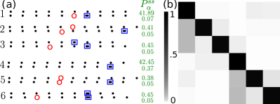
Figure 3: (a) Selection of microstates inside the six macrostates identified with PCCA+: the atoms positions relative to potential minima (black dots) display kinks (red circles) and anti-kinks (blue squares). For clarity, the probability $P_{\alpha}^{\rm ss}$ is multiplied by $100$, and we show only $12$ of the $\sim 100$ microstates. (b) Representation of the reduced transition matrix $\widetilde{\Pi}_{\alpha\beta}$ (grey scale proportional to magnitude, see text).

Macrostates $\tilde{c}_{1}$ and $\tilde{c}_{4}$ include the relaxed chain microstates, along with some single excitations at the tips; $\tilde{c}_{2}$ and $\tilde{c}_{5}$ contain mostly single kinks, while $\tilde{c}_{3}$ and $\tilde{c}_{6}$ contain mostly anti-kinks. The microstates with (kink, anti-kink) pairs are spread between groups, with neighboring pairs belonging to $\tilde{c}_{1,4}$ and extended pairs to others. The only difference between the triplets of $\tilde{c}_{1,2,3}$ and $\tilde{c}_{4,5,6}$ is in the value of $x_{\rm CM}$, respectively $x_{\rm CM}\approx 0.15$ and $1.15$. Overall, this description provides a qualitative understanding of the basic mechanisms of slips complementary to that of our kinetic analysis, and allows to directly read the kink and antikink populations as the collective variables describing sliding. The $6\times 6$ TM $\widetilde{\Pi}_{\alpha\beta}$ (Fig. 3(b)) shows, e.g., that motion (looping through states) occurs only through excited states $\tilde{c}_{2,3;5,6}$. Additional details about the role of each macrostate is given in the SI sec. 2.3.

Macrostate evolution, benchmarking — In the macrostate representation, the probabilities $P_{\alpha}^{t}=P(X^{t}\in\tilde{c}_{\alpha})$ evolve in time as $P_{\alpha}^{t+\tau}=\widetilde{\Pi}_{\alpha\beta}P_{\beta}^{t}$. For the whole construction to be satisfactory, this coarse-grained evolution should reproduce the quantitative aspects of the frictional dynamics of the raw data (before clustering). To this effect, we compare the work distribution $P^{\rm ss}(W)$ in the raw data with that of the steady state relative to $\widetilde{\Pi}_{\alpha\beta}$, where each $\tilde{c}_{\alpha}$ is associated to the distribution $P(O|\alpha)$ within the configurations belonging to $\tilde{c}_{\alpha}$. Results in Fig. 4(a) confirm that the stationary work distribution in the reduced model matches well the raw distribution. The particle current in the reduced basis is $\langle J\rangle=6.82\cdot 10^{-4}$, compared with the exact $\langle J\rangle=6.66\cdot 10^{-4}=v_{\rm ext}/a$. A similar agreement is found for the center of mass ($x_{\rm CM}$) dynamics and other observables. The steady state and excitation modes $g_{i}(x_{\rm CM})$ reproduce well those of the $n_{c}$ states description (see Fig. 4(b) and SI Fig. 4).

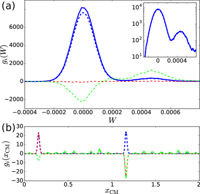
Figure 4: Comparison of (a) work $g_{i}(W)$ and (b) center of mass $g_{i}(x_{\rm CM})$ distributions for $i=1,2,3$ (blue, red, green). Solid lines: raw data; dashed lines: $\tilde{n}_{c}=6$ macrostate results. Inset: blowup of $g_{i}(W)$, highlighting the excess probability for $W>0$, signaling the positive frictional work. Note how $i=3$ (green) is the excitation of the steady state (blue) that populates the $W>0$ tail. In (b), the $i=2$ (red) excitation simply shifts the chain by $a$.

The lifetimes corresponding to these modes, and more precisely the decay of the correlation functions of various observables also match well the respective correlation functions evaluated on the raw data.

Conclusions — We formulated and carried out the first analysis of frictional sliding conducted through the MSM method extended to non-equilibrium. After an initial choice of metric for the phase space, the approach builds in an unbiased manner a still large but limited number of microstates that allow to track the effective dynamical variables of a sliding problem. Using the standard PCCA+ approach, one then derives a reduced dynamics in only a handful of macrostates. In the chosen FK model implementation the method works well, and the coarse-graining is sharp enough to capture not only overall steady-state observables such as average dissipated power or average current, but also their modes of excitations and their correlations, as shown by the excitations $g_{i}(O)$. In this way all the important, slow dynamical features can be brought under control in a manner which is, as far as we know, unprecedented for violent, nonlinear frictional motion. Further developments to efficiently improve the statistical quality could introduce a biased sampling favouring the exploration of rare transition event states in cases where a long “ergodic” trajectory cannot be generated Chodera et al. (2007). This work opens a route towards a quantitative approach to frictional dynamics, in nanoscale sliding as well as in other driven systems.

Acknowledgments — Work carried out under ERC Advanced Research Grant N. 320796 – MODPHYSFRICT. FL thanks R. Dandekar for useful discussions.

Supplementary material to Markov State Modeling of Sliding Friction

I 1.1 Lagtime estimation

As usual in MSM models, we need to determine the range of lagtimes that are long enough to obtain markovianity, and thus a correct estimation of the dominant timescales, while still being shorter than the time scale of the most rapid events we want to describe.

In this perspective, we start by computing the first non-trivial time scales $\tau_{i},i>1$ (since $\tau_{1}=\infty$), for various lagtimes $\tau$. The definition of $\tau_{i}$ is $-\tau/\log(\lambda_{i})$. We neglect sample-to-sample variations in this first study, as they are relatively small for $\tau_{i},i<100$, compared to the dependence in $\tau$. From Figure 5 we see that the range of acceptable lagtimes is contained in $1-100$. In what follows, we will use $\tau=10$ unless explicitly stated, since this value lies in the center of the range.

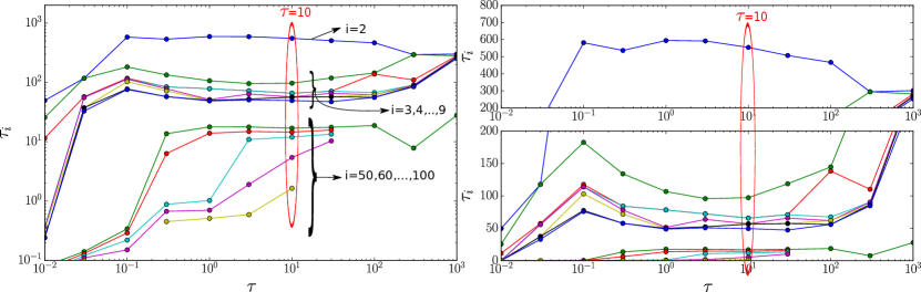
Figure 5: Timescales $\tau_{i}=1/\log(\lambda_{i})$ for a couple of representative $i$ values (as labeled), as a function of the choice of lagtime $\tau$, obtained from the TM of the clustering. Left: doubly logarithmic scale; Right: linear scale in $\tau_{i}$. There is a clear plateau for all time scales $i\leq 60$ in the range $\tau\in[0.5,50]$. Right: same plot in semi-log coordinates, to show the details of fluctuations around the chosen value, $\tau=10$.

Because the sample size $N=10^{5}$ is still too small for the phase space to be uniformly explored, the spectra fluctuate between the sets of $N$ configurations. To assess the reliability of these spectra, we average across 10 sets of $N$ configurations and compute the standard deviation of the results (see figure 6).

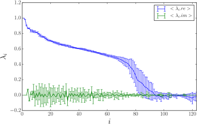
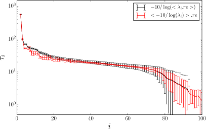
Figure 6: Full eigenvalue spectra (left) and timescale distribution (right) depending on the lagtime, using lagtimes $\tau=10$. They are fairly stable for $\tau\approx 10$. The error bars show the standard deviation.

Note that figure 2 of the main text was obtained using this average.

II 2 PCCA+

II.1 2.1 Short presentation

The key idea underlying standard PCCA Deuflhard et al. (2007) is that the TM relative to a group of $\tilde{n}_{c}$ disconnected (i.e. separate, independent) Markov chains is block-diagonal: the Perron eigenvalue $\lambda=1$ has degeneracy $\tilde{n}_{c}$ and the first $\tilde{n}_{c}$ (right) eigenvectors $\chi_{\alpha}$ map to membership functions $\xi_{\alpha}$ that are indicator functions, $(\xi_{\alpha})_{j}=\{0,1\}$ ($1$ for all the states $j$ that belong to the Markov chain $\tilde{c}_{\alpha}$ and $0$ elsewhere). These $\xi_{\alpha}$’s are found by following the sign structure of the $\chi_{\alpha}$’s.

A more advanced version, the Robust Perron Cluster Cluster Analysis (PCCA+) Deuflhard and Weber (2005); Weber and Kube (2005) makes use of fuzzy sets, i.e. membership functions become probabilities: $\sum_{j}(\xi_{\alpha})_{j}=1$ ($(\xi_{\alpha})_{j}\geq 0$). To find these $\xi_{i}$’s, one has to optimize a regular matrix $\mathcal{A}$ linking the $\tilde{n}_{c}$ membership vectors $\xi_{\alpha}$ to the $n_{c}$ eigenvectors $\chi_{i}$: $\widehat{\xi}=\mathcal{A}\widehat{\chi}$ ($\widehat{\chi}$ denotes the matrix of all eigenvectors, $\widehat{\xi}$ that of all membership vectors). The microstate $j$ is then assigned to the cluster ${\text{argmax}_{\alpha}}[(\xi_{\alpha})_{j}]$, and we obtain the TM after re-clustering, $\widetilde{\Pi}_{\alpha\beta}$. We must optimize $\mathcal{A}$ with respect to some cost function, usually $J_{1}=\sum_{j}{\text{max}_{\alpha}}[(\xi_{\alpha})_{j}]$ or $J_{2}=Tr(\mathcal{A})=\sum_{\alpha}\widetilde{\Pi}_{\alpha\alpha}$, in the space of possible matrices $\mathcal{A}$. Intuitively, the quality functions $J_{1}$ is the sum over the $\tilde{n}_{c}$ macrostates of the assignation probability of the microstate $c_{\alpha}$ that is assigned with best confidence, i.e. it makes sure that each macrostate has at least one microstate that is assigned to it with large probability. Conversely $J_{2}$ measures the metastability of each final macrostate: it is the sum of the weights of self-links in the final $\tilde{n}_{c}\times\tilde{n}_{c}$ graph (the trace of the final $\tilde{n}_{c}\times\tilde{n}_{c}$ transition matrix). We optimized $J_{2}$, but results do not significantly change if we optimize $J_{1}$.

Applying PCCA+ on a couple of clustering of $N=10^{5}$ configurations, each with $n_{c}\sim 100$ clusters, we identify $\tilde{n}_{c}=6$ as the optimal number of macrostates for $L=10$, and $\tilde{n}_{c}=5$ or $6$ for $L=15$: see Fig. 7.

Note that to give a decent weight to the center of mass, we define the distance between configurations at times $s$ and $t$ as:

$$d_{st}=\left(x^{s}_{\rm CM}-x^{t}_{\rm CM}\right)_{\text{mod }2}^{2}+\frac{10}{L}\sum_{l=1}^{L-1}\left(b^{s}_{l}-b^{t}_{l}\right)^{2},$$

which is consistent with the main text definition (for which we had $L=10$).

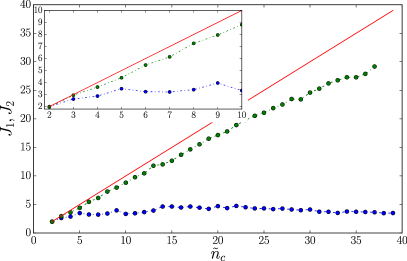
Figure 7: Cost functions $J_{1}$ and $J_{2}$ as a function of the number of macrostates $\tilde{n}_{c}$ in which we ask the clusters to be re-grouped. Both are bounded by $\tilde{n}_{c}$ (red line). The PCCA+ is applied on the clustering for two lengths of the chain, $L=10$ (left) and $L=15$ (right). We note that $J_{2}$ does not depend strongly on $\tilde{n}_{c}$ (it increases almost as its upper bound). $J_{1}$ has relative maxima in $6$ (for $L=10$) and 6 or 5 (for $L=15$). We pick $\tilde{n}_{c}=6$ macrostates as being the largest $\tilde{n}_{c}$ that still optimizes $J_{1}$. The lagtime used is $\tau=10$.

Note that the original PCCA+ algorithm is intended to be used on equilibrium problems, where the TM is symmetric. Here it is not the case, and we symmetrize the matrix for simplicity. A more refined approach would be to use a Schur decomposition of the TM instead of a direct diagonalization, as was proposed in Roeblitz (2009) and performed in detail in Conrad et al. (2015). As results are already satisfying here, we kept with standard PCCA+: this simply overestimates some rates of exchange, and make the rates of staying in a microstate relatively smaller. This illustrates the robustness of the method, since despite this approximation, we still detect well the relevant macrostates.

We implemented PCCA+ using available code (https://github.com/msmbuilder/msmbuilder/) Deuflhard and Weber (2005); Kube et al. (2007); Roeblitz (2009); Deuflhard et al. (2007) as a basis, but integrated it in our toolbox, allowing the user to estimate a correct lagtime $\tau$ and compute the optimal $\tilde{n}_{c}$ in an easy way. Our version of the code is available at Cod (2016), together with the codes for integrating the FK model’s equations and the density peak algorithm.

The work distribution for the chain lengths $L=15,20$, and its excitation modes are shown in Fig. 8. They are interpreted in the same way as those of Fig. 4 of the main text. Note the robustness of the $\tilde{n}_{c}=6$ macrostate description relative to the variable $L$: the first $3$ modes are basically invariant under changes in system size.

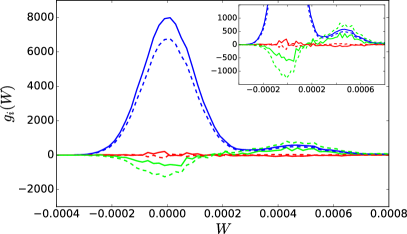
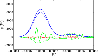
Figure 8: Comparison of work distribution $g_{i}(W)$ for $i=1,2,3$ (blue, red, green) for $L=15$ (left) and $L=20$ (right), using $\tilde{n}_{c}=6$ in both. Solid lines: $n_{c}\sim 100-300$ microstate results; Dashed lines: $\tilde{n}_{c}=6$ macrostate results.

II.2 2.2 Further lagtime assessment

One can further assess the quality of the lagtime by checking the dependence of the five timescales (since $\tilde{n}_{c}=6$) of the lumped model, obtained after applying PCCA+ to the clustering, together with the lifetime of staying in the most probable state (i.e. the relaxed chain, which can have either an odd or even center of mass position). We see in Figure 9 that indeed the variations in all these timescales are small. Our choice $\tilde{n}_{c}=6$ is confirmed by the study of lagtime dependence: for larger $\tilde{n}_{c}$, the plateaus quickly deteriorate (not shown).

Figure 9: Time scales after lumping by PCCA into $\tilde{n}_{c}=6$ macrostates. Red squares show the lifetime of staying in the most probable of the $\tilde{n}_{c}$ states. For the lagtime $\tau=10$ we have 10 independent realizations (left), which show little fluctuations. (for a chain of $L=10$ atoms).

II.3 2.3 Further characterization of the lumping obtained by PCCA+

The Fig. 3 of the main text does not show all the clusters assigned by the PCCA+, as there are too many. To give a more complete view of how the PCCA+ lumps the clusters we found, we provide a complete description of these states in Fig. 10. In particular, we define the rescaled chain length (shifted by $-L$), which thus takes values between $-1$ and $1$. We also define a quantity $k$, or KinkCount, which is a proxy for the number of defects, $k=\sum_{l=1}^{L-1}(b_{l})^{2}$, which was identified as the main collective variable. The position of the center of mass $x_{\rm CM}$ was defined in the text. We also show the assignation probability of each microstate $j$ to the macrostate $\alpha$ it was affected to, i.e. the value of $p={\text{max}_{\alpha}}[(\xi_{\alpha})_{j}]$. A high value indicates that the assignation was done with high confidence, while a low value means that this assignation is not robust. The weight $w=100P_{j}^{ss}$ represents the steady state probability to be in the microstate $j$ (we can take this probability according to the raw data statistics or according to $\Pi_{\alpha\beta}$, in our case it is the same, because the clustering works very well). These weights $w$ sum to $100$, for clarity’s sake.

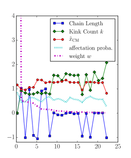
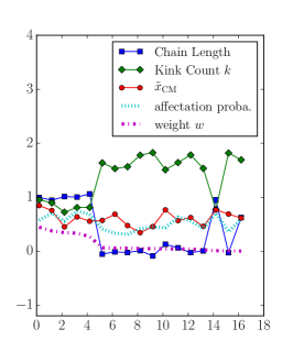
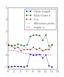
Figure 10: Each panel corresponds to a group: from left to right, $g=1,2,3$ (following the main text labels). In each group, we show the value of the chain length for each microstate (shifted by $-L$), the kinkCount measure, the center of mass position $\tilde{x}_{{\rm CM}}$ (rescaled and modulo 2), the assignation probability provided by the PCCA+ method, and the microstate’s global weight $w$ (summing them all gives 100). There are 121 microstates, before lumping.

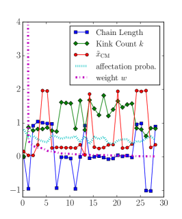
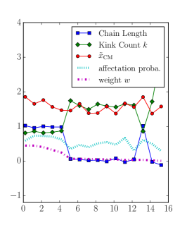
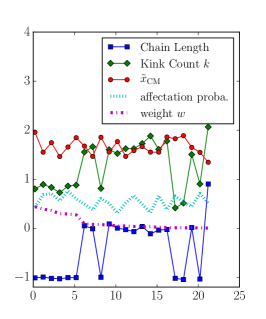
Figure 11: Continuation of Fig. 10 but for the lumps with the other parity (other value of the center of mass): here the groups are $g=4,5,6$ (left to right). Note that these 3 panels are extremely similar to the three above, as expected, except of course for the center of mass position, which is around $0.15$ (or $2$ because of periodicity) in one case and around $1.15$ in the other.

References

- Gnecco and Meyer (2015) E. Gnecco and E. Meyer, NanoScience and Technology (2015).
- Schwantes et al. (2014) C. R. Schwantes, R. T. McGibbon, and V. S. Pande, The Journal of Chemical Physics 141, 090901 (2014).
- Noé and Nüske (2013) F. Noé and F. Nüske, Multiscale Modeling & Simulation 11, 635 (2013).
- Bowman et al. (2014) G. R. Bowman, V. S. Pande, and F. Noé, in An Introduction to Markov State Models and Their Application to Long Timescale Molecular Simulation (2014), vol. 797.
- Schütte and Sarich (2015) C. Schütte and M. Sarich, The European Physical Journal Special Topics 18 (2015).
- Wang and Schütte (2015) H. Wang and C. Schütte, Journal of Chemical Theory and Computation 11, 1819 (2015).
- Frenkel and T A Kontorova (1938) Y. I. Frenkel and T A Kontorova, Phys. Z. Sowietunion 13 (1938).
- Braun and Kivshar (1998) O. M. Braun and Y. S. Kivshar, Physics Reports 306, 1 (1998).
- Paliy et al. (1997) M. Paliy, O. Braun, T. Dauxois, and B. Hu, Physical Review E 56, 4025 (1997).
- Rodriguez and Laio (2014) A. Rodriguez and A. Laio, Science (New York, N.Y.) 344, 1492 (2014).
- Deuflhard and Weber (2005) P. Deuflhard and M. Weber, Linear Algebra and its Applications 398, 161 (2005).
- Weber and Kube (2005) M. Weber and S. Kube, Lecture Notes in Computer Science 3695, 57 (2005).
- Vanossi et al. (2013) A. Vanossi, N. Manini, M. Urbakh, S. Zapperi, and E. Tosatti, Reviews of Modern Physics 85, 529 (2013).
- Cod (2016) https://bitbucket.org/flandes/msm_fk_densitypeakalgo_rpcca/ (2016).
- Roeblitz (2009) S. Roeblitz, Ph.D. thesis, Statistical Error Estimation and Grid-free Hierarchical Refinement in Conformation Dynamics Freie Universität Berlin (2009).
- Conrad et al. (2015) D. N. Conrad, M. Weber, and C. Schütte, 40 (2015).
- Chodera et al. (2007) J. D. Chodera, N. Singhal, V. S. Pande, K. a. Dill, and W. C. Swope, Journal of Chemical Physics 126, 1 (2007).
- Deuflhard et al. (2007) P. Deuflhard, W. Huisinga, A. Fischer, and Ch. Schütte, Linear Algebra and its Applications 315, 39–59 (2000).
- Kube et al. (2007) S. Kube, and M. Weber, Journal of Chemical Physics 126, 024103 (2007).