Generating Point Configurations via Hypersingular Riesz Energy With an External Field

Abstract.

For a compact $d$-dimensional rectifiable subset of $\mathbb{R}^{p}$ we study asymptotic properties as $N\to\infty$ of $N$-point configurations minimizing the energy arising from a Riesz $s$-potential $1/r^{s}$ and an external field in the hypersingular case $s\geq d$. Formulas for the weak^∗ limit of normalized counting measures of such optimal point sets and the first-order asymptotic values of minimal energy are obtained. As an application, we derive a method for generating configurations whose normalized counting measures converge to a given absolutely continuous measure supported on a rectifiable subset of $\mathbb{R}^{p}$. Results on separation and covering properties of discrete minimizers are given. Our theorems are illustrated with several numerical examples.

1. Introduction

We are concerned with the problem of minimizing the discrete Riesz $s$-energy of $N$ particles constrained to a compact subset $A$ of $\mathbb{R}^{p}$ of Hausdorff dimension $d$ under the influence of an external field $q(x)$. More precisely, we minimize

(1.1) $$E^{q}_{s,d}(\omega_{N}):=\sum_{\begin{subarray}{c}x\neq y\\ x,y\in\omega_{N}\end{subarray}}|x-y|^{-s}+\frac{\tau_{s,d}(N)}{N}\,\sum_{x\in\omega_{N}}q(x),\quad s\geq d,$$

for

(1.2) $$\tau_{s,d}(N):=\begin{cases}N^{1+s/d},\ &s>d,\\ N^{2}\log N,\ &s=d,\end{cases}$$

over $N$-element subsets $\omega_{N}\subset A$.

The factor $\tau_{s,d}(N)/N$ is chosen so that the two terms on the right hand side of (1.1) have the same order of growth as $N\to\infty$. Here we consider only the case when $s$ is chosen greater than or equal to the dimension of the set $A$ because for $s<d$ such external field problems come under the umbrella of classical potential theory and have been well studied as we describe below.

One motivation to consider this energy expression is that (under mild conditions on the set $A$) for any probability measure $\mu$ on $A$ that is absolutely continuous with respect to the $d$-dimensional Hausdorff measure restricted to $A$, there is an easily described external field $q(x)$ for which the normalized counting measures of the minimizers of (1.1) weak^∗ converge to $\mu$ (formal definitions are given in the next two subsections).

For $s>d$ the minimizers of (1.1) are shown to have optimal orders of separation and covering as $N\to\infty$. Minimization of (1.1) therefore provides well-distributed nodes on compact sets, which can be used for a number of applications; for example, meshless methods [22], halftoning [27] and sensor deployment [17].

External fields arise in the Gauss variational problem, which involves minimizing the functional

(1.3) $$I_{\kappa,q}(\mu):=\iint\limits_{A\times A}\kappa(x,y)\,\mathrm{d}\mu(x)\,\mathrm{d}\mu(y)+2\int_{A}q(x)\,\mathrm{d}\mu(x),$$

for a pair of fixed integrable lower semi-continuous functions $\kappa:A\times A\to{\mathbb{R}\cup\{+\infty\}},\ q:A\to\mathbb{R}\cup\{+\infty\}$ over the probability measures supported on $A$. The classical work of Ohtsuka [23] deals with this question when $A$ is locally compact. The case $\kappa(x,y)=\log\frac{1}{|x-y|}$ and a number of its applications to constructive analysis are extensively treated in the book [26] by Saff and Totik. More recently, the question of solvability of the Gauss variational problem was considered by Zorii in [28] and [29].

The discrete form of (1.3) is the problem of minimization over all $N$-element sets $\omega_{N}\subset A$ of

(1.4) $$E_{\kappa,q}(\omega_{N})=\sum_{\begin{subarray}{c}x\neq y\\ x,y\in\omega_{N}\end{subarray}}\kappa(x,y)+N\sum_{x\in\omega_{N}}q(x),\qquad N=1,2,\ldots.$$

Such problems have been studied by Petrache, Rougerie and Serfaty in [24], [25] for the Riesz $s$-kernel

(1.5) $$\kappa_{s}(x,y):=|x-y|^{-s},$$

with $s<d$, and for the logarithmic kernel in [26]. An earlier series of papers [12], [8] and [9] by Brauchart et al. explores minima of (1.4) when $A$ is a $d$-dimensional sphere and $d-2\leq s<d$. The paper [4] by Bilogliadov considers minimizing (1.3) with the Riesz kernel for $s=1$ and a rotationally symmetric $q$ over probability measures supported on the $2$-dimensional unit sphere.

1.1. Hypersingular Riesz kernels

We call the Riesz kernels $\kappa_{s}(x,y)=|x-y|^{-s}$ hypersingular when $s\geq d=\dim A$, and deal only with this case from now on. The reason to consider such kernels will become evident from the following result, which shows that the minimizers of (1.1) with $q\equiv 0$ are well-distributed on the set $A$, which need not to be the case when $s<d$.

For the purposes of studying the asymptotic behavior of $N$-point configurations $\omega_{N}$ on $A$ we consider their normalized counting measures. Recall that such measures $N^{-1}\sum_{x\in\omega_{N}}\delta_{x}$ are said to weak^∗ converge to the measure $\lambda$ if

(1.6) $$\forall f\in C(A),\qquad\frac{1}{N}\sum_{x\in\omega_{N}}f(x){\longrightarrow}\int f\,\mathrm{d}\lambda\quad\text{ as }N\to\infty,$$

where, as usual, $C(A)$ denotes the family of all continuous functions defined on $A$. Weak^∗ convergence is denoted by $\stackrel{{\scriptstyle*}}{{\longrightarrow}}$.

We further need to impose some regularity conditions on the underlying compact set. A set $A\subset\mathbb{R}^{p}$ is said to be $d$-rectifiable if it is the image of a bounded subset of $\mathbb{R}^{d}$ under a Lipschitz mapping. Note that any subset of a $d$-rectifiable set is also $d$-rectifiable. Here and below we write $\mathbb{B}^{d}$ for the $d$-dimensional unit ball. We use $\mathcal{H}_{d}$ to denote the $d$-dimensional Hausdorff measure on $\mathbb{R}^{p}$ normalized so that $[0,1]^{d}\subset\mathbb{R}^{d}\subset\mathbb{R}^{p}$ has unit volume, and by $\mathcal{H}_{d}^{A}$ its restriction to $A$. In particular, for a $d$-rectifiable $A$, $\mathcal{H}_{d}(A)<\infty$. The following theorem concerns a variant of (1.1) without external field:

(1.7) $$\mathcal{E}_{s}(A,N):=\inf_{\omega_{N}\subset A}E_{s}(\omega_{N}),$$

where $E_{s}(\omega_{N}):=\sum_{x\neq y\in\omega_{N}}\kappa_{s}(x,y)$. This infimum is attained for compact sets $A$, because the Riesz $s$-kernel is lower semi-continuous on $A\times A$.

Theorem A ([15],[6]).

Suppose $s\geq d$ and $A\subset\mathbb{R}^{p}$ is $d$-rectifiable and compact. If $s=d$, it is further assumed that $A$ is a subset of a $d$-dimensional $C^{1}$ manifold. Then for $s=d$

(1.8) $$\lim_{N\to\infty}\frac{\mathcal{E}_{s}(A,N)}{N^{2}\log N}=\frac{\mathcal{H}_{d}(\mathbb{B}^{d})}{\mathcal{H}_{d}(A)},$$

while for $s>d$, the following limit exists:

(1.9) $$\lim_{N\to\infty}\frac{\mathcal{E}_{s}(A,N)}{N^{1+s/d}}=\frac{C_{s,d}}{\mathcal{H}_{d}(A)^{s/d}},$$

where $C_{s,d}$ is a finite positive constant independent of $A$ and $p$, and $1/0=+\infty$. Furthermore, if $\mathcal{H}_{d}(A)>0$ and $\{\omega_{N}\}_{N\geq 2}$ is any sequence of $N$-point configurations on $A$ satisfying

(1.10) $$\lim_{N\to\infty}\frac{E_{s}(\omega_{N})}{\mathcal{E}_{s}(A,N)}=1,$$

then

(1.11) $$\frac{1}{N}\sum_{x\in{\omega}_{N}}\delta_{x}\stackrel{{\scriptstyle*}}{{\longrightarrow}}\frac{\,\mathrm{d}\mathcal{H}_{d}^{A}}{\mathcal{H}_{d}(A)},\quad N\to\infty.$$

This theorem is sometimes described as the Poppy-seed bagel theorem, a name that alludes to discrete equilibrium configurations on the torus. It first appeared in [15, Theorem 2.1], and in the present generality in [6, Theorems 1–3].

In particular, the theorem holds for any compact $A\subset\mathbb{R}^{d}$ as well as any compact subset of a smooth $d$-dimensional manifold. To be consistent with the notation of (1.9), we define $C_{d,d}$ according to (1.8):

(1.12) $$C_{d,d}:={\mathcal{H}_{d}(\mathbb{B}^{d})}=\frac{\pi^{d/2}}{\Gamma\left(d/2+1\right)},\quad d\geq 1,$$

where $\Gamma$ is the standard gamma function. It is known for $d=1,\ s>1$ that

(1.13) $$C_{s,1}=2\zeta(s), \quad s>1,$$

where $\zeta$ is the Riemann zeta function, see e.g. [20]. However, for dimensions $d\geq 2$ the exact value of $C_{s,d}$ is unknown. In the cases $d=2,\ 4,\ 8,\ 24$, the conjectured value is

(1.14) $$C_{s,d}=|\Lambda_{d}|^{s/d}\zeta_{\Lambda_{d}}(s),\ \quad s>d,$$

where $\Lambda_{d}$ denotes, respectively, the hexagonal, $D_{4},\ E_{8}$ and Leech lattices; $|\Lambda_{d}|$ is the volume of its fundamental cell; and $\zeta_{\Lambda_{d}}$ is the corresponding Epstein zeta-function; see [10, Conjecture 2]. As shown in [10, Proposition 1], the conjectured values (1.14) serve as upper bounds for their respective $C_{s,d}$.

One way of generalizing Theorem A so that it yields non-uniform limiting distributions was studied in [6], where the Riesz potential is multiplied by a weight satisfying semicontinuity conditions. More precisely, one minimizes the energy

$$E^{w}_{s}(\omega_{N}):=\sum_{x\neq y\in\omega_{N}}\frac{w(x,y)}{|x-y|^{s}},$$

for a non-negative weight function $w$ on $A\times A$. Our present goal is to develop an alternate approach by introducing an external field equipped with a suitable scaling factor that depends on the number of points $N$.

With regards to practical implementation, it is worth mentioning that by using a localized weight $w(\cdot,\cdot):=w_{N}(\cdot,\cdot)$ that depends on the number of points, one can lower the computational complexity of $E^{w}_{s}(\omega_{N})$. This approach is investigated in [7]. On the other hand, a number of papers are dedicated to producing well-distributed discrete configurations by drawing them from a suitable random process with, perhaps, further local optimization, see for example [1], [2], [19]. The possibility of introducing a multiplicative weight together with an external field, as well as decreasing the complexity of the method described below will be the subject of a future work.

The outline of the paper is as follows. In the remaining part of this section we introduce some essential notation. Section 2 contains an extension of the Poppy-seed theorem to the case when an external field is present; it also includes results on separation and covering of minimizing configurations. We discuss numerical examples in Section 3. Finally, Section 4 contains proofs of the results stated in Section 2.

1.2. Notation

We consider configurations of points restricted to a compact set $A\subset\mathbb{R}^{p}$, such that $\mathcal{H}_{d}(A)>0$, $d\leq p$. The external field $q:A\to(-\infty,\infty]$ is assumed to be lower semi-continuous and finite on a subset of $A$ of positive $\mathcal{H}_{d}^{A}$-measure. We write $\mathring{M}$ for the interior of a set $M\subset\mathbb{R}^{p}$, and $\overline{M}$ for its closure. For a real number $r$, let $(r)_{+}:=\max(0,\,r)$. The closed ball in $\mathbb{R}^{p}$ of radius $r$ centered at the point $x$ is denoted by $B(x,r)$. Notation $L^{1}(A,\lambda)$ stands for the class of functions integrable on the set $A$ with respect to measure $\lambda$.

The minimal $(s,d,q)$-energy of the set $A$ over all $N$-point subsets of $A$ is given by

(1.15) $$\mathcal{E}_{s,d}^{q}(A,N):=\inf\{E^{q}_{s,d}(\omega_{N}):\omega_{N}\subset A,\ \#\omega_{N}=N\},$$

where $\#S$ denotes the cardinality of a set $S$. Since $q$ is lower semi-continuous and $A$ is compact, there exists a configuration of $N$ charges $\hat{\omega}_{N}$ for which the infimum in (1.15) is attained; i.e.,

$$E^{q}_{s,d}(\hat{\omega}_{N})=\mathcal{E}_{s,d}^{q}(A,N).$$

Such a configuration $\hat{\omega}_{N}$ will be called an $N$-point $(s,d,q)$-energy minimizer on $A$.

2. Main results

2.1. A Poppy-seed theorem for $\boldsymbol{(s,d,q)}$-energy

The following two results extend Theorem A to $(s,d,q)$-energy.

Theorem 2.1.

Assume $0<d\leq p$, and $s\geq d$. Let $A\subset\mathbb{R}^{p}$ be a $d$-rectifiable compact set, $\mathcal{H}_{d}(A)>0$, and in the case $s=d$ require additionally that $A$ be a subset of a $d$-dimensional $C^{1}$-manifold. Further assume that $q$ is a lower semi-continuous function on $A$ and finite on a set of positive $\mathcal{H}_{d}^{A}$-measure. Define $L_{1}$ and $\mu_{A}^{q}$ to be the positive constant and probability measure determined, respectively, by

(2.1) $$\int\left(\frac{L_{1}-q(x)}{C_{s,d}(1+s/d)}\right)^{d/s}_{+}\,\mathrm{d}\mathcal{H}_{d}^{A}(x)=1,\qquad\,\mathrm{d}\mu_{A}^{q}:=\left(\frac{L_{1}-q(\cdot)}{C_{s,d}(1+s/d)}\right)^{d/s}_{+}\,\mathrm{d}\mathcal{H}_{d}^{A},$$

where $C_{s,d}$ for $s\geq d$ is the same as in Theorem A. Then

(2.2) $$\lim\limits_{N\to\infty}\frac{\mathcal{E}_{s,d}^{q}(A,N)}{\tau_{s,d}(N)}=S(q,A):=\int\limits\frac{L_{1}+sq(x)/d}{1+s/d}\,\,\mathrm{d}\mu_{A}^{q}(x).$$

Furthermore, if $\{{\omega}_{N}\}_{N\geq 2}$ is any sequence of asymptotically $(s,d,q)$-energy minimizing configurations on $A$; that is,

(2.3) $$\lim_{N\to\infty}\frac{E^{q}_{s,d}(\omega_{N})}{\tau_{s,d}(N)}=S(q,A),$$

then

(2.4) $$\frac{1}{N}\sum_{x\in{\omega}_{N}}\delta_{x}\stackrel{{\scriptstyle*}}{{\longrightarrow}}\,\mathrm{d}\mu_{A}^{q}\quad\text{ as }N\to\infty.$$

Remark 2.2.

As with Theorem A, this result holds on the (possibly) larger class of sets $A$ satisfying $\mathcal{H}_{d}(A)=\mathcal{M}_{d}(A)$, where $\mathcal{M}_{d}$ is the $d$-dimensional Minkowski content.

As an application of Theorem 2.1, we deduce a method for constructing a sequence of $(s,d,q)$-energy minimizing collections $\hat{\omega}_{N}$ such that their normalized counting measures weak^∗ converge to a given distribution.

Theorem 2.3.

Let the assumptions of Theorem 2.1 on the set $A$ and numbers $s,d,p$ hold. Assume further $\rho:A\to[0,\infty)$ is an upper semi-continuous function, such that $\rho\,\mathrm{d}\mathcal{H}_{d}^{A}$ is a probability measure. Then the lower semi-continuous function $q:A\to\left(-\infty,0\right]$ given by

(2.5) $$q(x):=-M_{s,d}\rho(x)^{s/d},\quad\text{where }M_{s,d}:=C_{s,d}(1+s/d),$$

is such that any sequence $\{\hat{\omega}_{N}\}_{N\geq 2}$ of $(s,d,q)$-energy minimizers converges weak^∗ to $\rho\,\mathrm{d}\mathcal{H}_{d}^{A}$:

(2.6) $$\frac{1}{N}\sum_{x\in\hat{\omega}_{N}}\delta_{x}\stackrel{{\scriptstyle*}}{{\longrightarrow}}\rho\,\mathrm{d}\mathcal{H}_{d}^{A},\quad N\to\infty.$$

In particular, for $s=d$ equation (2.6) holds with (2.5) taking the form

(2.7) $$q(x):=-\frac{2\pi^{d/2}\rho(x)}{\Gamma\left(d/2+1\right)}.$$

Remark 2.4.

The reader will no doubt observe that except for the case $d=1$ which is covered in (1.13), the usefulness of the last theorem is limited by the lack of knowledge of the value of $C_{s,d}$ when $d\geq 2$. Fortunately, the limit distribution in equation (2.6) is stable under perturbations of the constant $M_{s,d}$: small error in the value of $C_{s,d}$ used in (2.5) only leads to small errors in the resulting weak^∗ limit of minimizers. We quantify this statement in Proposition 2.5 below.

Another possible way of overcoming this difficulty is modifying the problem of minimizing (1.1) so that the charges are restricted to an unbounded set $A$. It will be addressed in a future work.

Proposition 2.5.

Assume that in Theorem 2.3 one uses an approximate value of $C_{s,d}$ satisfying

$$C_{s,d}^{\prime}=(1+\Delta)C_{s,d}$$

with a fixed $\Delta$. Let also $\rho(x)\geq\delta>0$ for all $x\in A$ and write $q^{\prime}(x)$ for the external field defined with $C_{s,d}^{\prime}$ instead of $C_{s,d}$ in (2.5). Then for $\Delta<{M_{s,d}}/\left({1+(\|\rho\|_{\infty}\delta^{-1})^{s/d}}\right)$, the weak^∗ limit of the $(s,d,q^{\prime})$-energy minimizers has density $\rho^{\prime}=\,\mathrm{d}\mu_{A}^{q^{\prime}}/\,\mathrm{d}\mathcal{H}_{d}^{A}$ satisfying

(2.8) $$|\rho^{\prime}(x)-\rho(x)|\leq\Delta\frac{d(1+\|\rho\|_{\infty}^{s/d}/\rho(x)^{s/d})}{sM_{s,d}}+o(\Delta),\qquad\Delta\to 0.$$

Example 2.6.

Consider the problem of minimization of $(4,1,q)$-energy on the interval $[0,2]$, where

$$q=(x-1)^{2}+\frac{1}{2}.$$

Formula (1.13) gives the exact value of $C_{4,1}$, which enables us to plot the density of $\mu_{[0,2]}^{q}$ on $[0,2]$. For comparison, we also plot the densities of asymptotic distributions obtained for non-exact values of $C_{4,1}$ by taking $\Delta=\pm 0.3,\pm 0.25,\pm 0.2,\pm 0.1,\pm 0.05,\pm 0.03$ in Proposition 2.5.

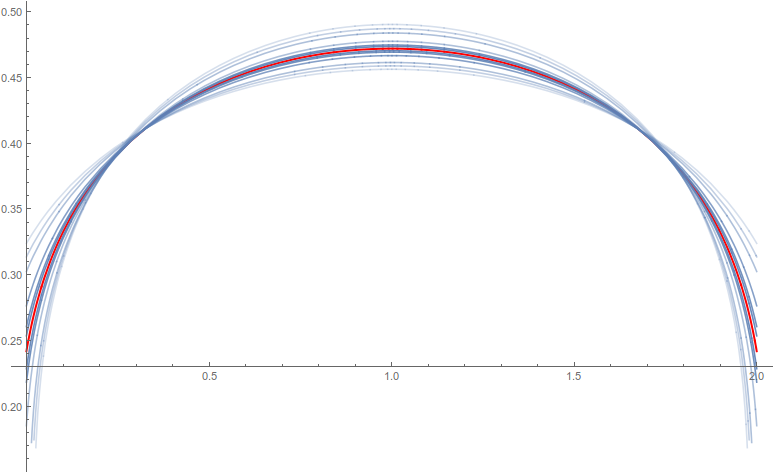
Figure 1. The exact graph of density $\,\mathrm{d}\mu_{[0,2]}^{q}$ is pictured in red, graphs for perturbed values of $C_{4,1}$ are in blue.

2.2. Separation and covering properties of minimal configurations

Let

$$\delta(\omega_{N}):=\min_{\begin{subarray}{c}x\neq y,\\ x,y\in\omega_{N}\end{subarray}}|x-y|,$$

be the separation distance of configuration $\omega_{N}$. We write $A(u):=\{x\in A:q(x)\leq u\}$ for a $u\in\mathbb{R}$.

Theorem 2.7.

Let $0<d\leq p$ and $s\geq d$. Let $A\subset\mathbb{R}^{p}$ be compact with $\mathcal{H}_{d}(A)>0$, and let $q$ be a nonnegative lower semi-continuous function on $A$. Then there exists a constant $C(A,s,d,q)$ such that for each $N$-point $(s,d,q)$-energy minimizer $\hat{\omega}_{N}\subset A$

$$\delta(\hat{\omega}_{N})\geq C(A,s,d,q)\begin{cases}N^{-1/d}&s>d,\\ (N\log N)^{-1/d}&s=d,\end{cases}\qquad N\geq 2.$$

To prove Theorem 2.7, we will need the following lemma which is also of independent interest. For a sequence of configurations $\{\omega_{N}\}_{N\geq 2}$ we consider the quantity

(2.9) $$U(x,\omega_{N}):=\sum_{\begin{subarray}{c}y\in{\omega}_{N}:\\ y\neq x\end{subarray}}|x-y|^{-s}+q(x)\tau_{s,d}(N)/N.$$

Lemma 2.8.

Let the assumptions of Theorem 2.7 be satisfied. Then there exists a constant $C(A,s,d,q)$ such that for every $(s,d,q)$-energy minimizing configuration $\hat{\omega}_{N},\ N\geq 2,$ and each $x\in\hat{\omega}_{N}$ there holds

(2.10) $$U(x,\hat{\omega}_{N})\leq C(A,s,d,q)\begin{cases}N^{s/d}&s>d;\\ N\log N&s=d,\end{cases}\qquad N\geq 2.$$

Corollary 2.9.

Let the assumptions of Theorem 2.7 hold. Then there exists a constant $C=C(A,s,d,q)$ such that for all $N\geq 2$, the minimizers $\hat{\omega}_{N}$ are contained in the set $A(C)$.

Due to this corollary, the sets $\{\hat{\omega}_{N}\}_{N\geq 2}$ for the problem of minimizing the $(s,d,q)$-energy on the whole space $\mathbb{R}^{d}$ are restricted to a compact set, provided that for some compact $A$ and a large enough cube $Q:=[-R,R]^{d}$ with $A\subset Q$, the value $C$ in (2.10) is such that $q(x)>C$ for any $x$ not in $Q$. Such a problem is then equivalent to energy minimization on $Q$ only.

To prove the covering property of $(s,d,q)$-energy minimizers, we will need the notion of Ahlfors regularity [11, Definition 1.13]. A set $A\subset\mathbb{R}^{p}$ with $\mathcal{H}_{d}(A)>0$ is called $d$-regular with respect to $\lambda$ if there are positive constants $c_{0},\ C_{0}$ and a positive locally finite Borel measure $\lambda$, such that

(2.11) $$c_{0}R^{d}\leq\lambda\big{(}B(x,R)\cap A\big{)}\leq C_{0}R^{d}$$

for all $x\in A$ and $0<R\leq\mathrm{diam}\,A$. In the case $\lambda=\mathcal{H}_{d}$, the set $A$ is called Ahlfors regular with dimension $d$.

For an $x\in A$ and an $N$-point collection $\omega_{N}$ define

$$\mathrm{dist}(x,{\omega}_{N}):=\min_{y\in{\omega}_{N}}|y-x|,$$

the covering radius at $x$ with respect to ${\omega}_{N}$.

Theorem 2.10.

Let $0<d\leq p$ and $s>d$. Assume $A\subset\mathbb{R}^{p}$ is compact, $d$-rectifiable and Ahlfors regular with dimension $d$. Assume also $q\geq 0$ is a continuous function. Let $x\in A(L_{1}-h)$ for some $h>0$, where $L_{1}$ is defined in Theorem 2.1. Then for each sequence of $(s,d,q)$-energy minimizers $\{\hat{\omega}_{N}\}_{N\geq 2}$, there exists a constant $C(A,h,s,d,q)$ such that

$$\mathrm{dist}(x,\hat{\omega}_{N})\leq C(A,h,s,d,q)N^{-1/d},\qquad N\geq 2.$$

A sequence of configurations $\{\omega_{N}\}_{N\geq 1}$ is said to be quasi-uniform in $M\subset A$ if the ratio

(2.12) $$\gamma(x;\omega_{N},A):=\mathrm{dist}(x,{\omega}_{N})/\delta(\omega_{N})$$

is bounded uniformly for all $x\in M$ and $N\geq 1$. From Theorems 2.7 and 2.10 we have the following result.

Corollary 2.11.

Let $s>d$. Assume $A\subset\mathbb{R}^{p}$ is compact, $d$-rectifiable and Ahlfors regular with dimension $d$. Suppose also that $q:A\to\mathbb{R}$ is a continuous function. Then for any sequence of $(s,d,q)$-energy minimizers $\{\hat{\omega}_{N}\}_{N\geq 2}$ on $A$, sequence of subsets $\{\hat{\omega}_{N}\cap A(L_{1}-h)\}_{N\geq 2}$ is quasi-uniform in $A(L_{1}-h)$ for any $h>0$. That is, for some constant $C=C(A,h,s,d,q)$ there holds:

$$\gamma(x;\omega_{N},A(L_{1}-h))\leq C(A,h,s,d,q),\qquad x\in A(L_{1}-h),\ N\geq 2.$$

3. Examples and numerics

All the results of this section were obtained by using default Mathematica routines (FindMinimum) to minimize the energy functional, starting with a randomly generated collection of point charges. We will write $L_{1}(q,A)$ to show explicitly the set on which we are solving the minimization problem and the external field acting on it.

In this section $\mathbf{e}_{z}:=(0,\ 0,\ 1)^{T}$ is the basis vector.

Example 3.1.

Consider the problem of minimizing (1.1) with $s=2$ and an external field

$$q_{\text{a}}(x)=\cos(3\arccos\langle x,\mathbf{e}_{z}\rangle)^{16}$$

on the unit sphere $\mathbb{S}^{2}\subset\mathbb{R}^{3}$. According to (1.12), $C_{2,2}=\pi$. Equation (2.1) for $L_{1}(q_{\text{a}},\mathbb{S}^{2})$ in this case is

(3.1) $$\int_{\mathbb{S}^{2}}\left(\frac{L-q_{\text{a}}(x)}{2\pi}\right)_{+}\,\mathrm{d}\mathcal{H}_{2}(x)=1,$$

solving it for $L$ gives $L_{1}(q_{\text{a}},\mathbb{S}^{2})\approx 0.65448$. Figure 2 is the graph of $q_{\text{a}}$ depending on $\langle x,\mathbf{e}_{z}\rangle$.

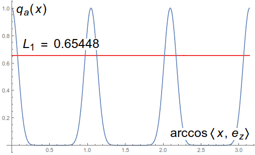
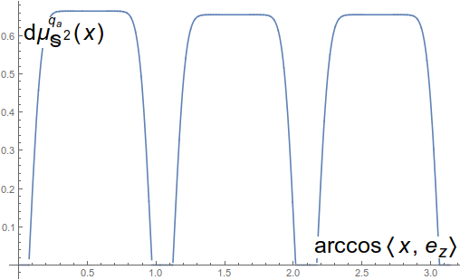
Figure 2. Left: graph of $q_{\text{a}}(x)$, right: $\,\mathrm{d}\mu_{\mathbb{S}^{2}}^{q_{\text{a}}}(x)$ from Example 3.1. The horizontal axis is $\arccos(\langle x,\mathbf{e}_{z}\rangle)$.

Density of $\mu_{\mathbb{S}^{2}}^{q_{\text{a}}}$ for this external field is

$$\,\mathrm{d}\mu_{\mathbb{S}^{2}}^{q_{\text{a}}}(x)=\left(\frac{L_{1}(q_{\text{a}},\mathbb{S}^{2})-\cos(3\arccos\langle x,\mathbf{e}_{z}\rangle)^{16}}{2\pi}\right)_{+}\,\mathrm{d}\mathcal{H}_{d}^{A}.$$

Using the numeric method described above, we obtain an approximate minimizer $\omega_{\text{a}}$ pictured in Figure 3.

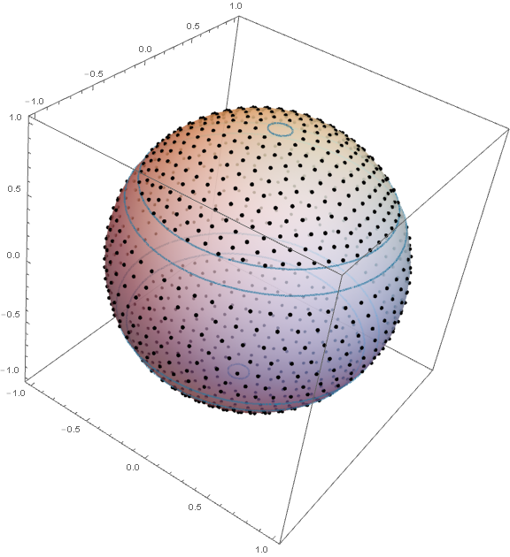
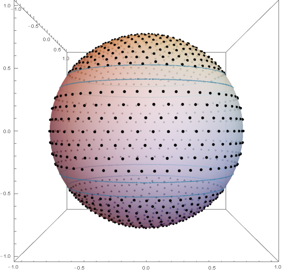
Figure 3. Two views of an approximate $1000$-point $(2,2,q_{\text{a}})$-energy minimizer $\omega_{\text{a}}$ from Example 3.1. The latitudinal circles denote the boundaries of $\operatorname{supp}\mu_{\mathbb{S}^{2}}^{q_{\text{a}}}$; i.e., $\{x:q_{\text{a}}(x)=L_{1}(q_{\text{a}},\mathbb{S}^{2})\}$.

Evaluating separation distance for $\omega_{\text{a}}$ gives $\delta(\omega_{\text{a}})\approx 0.0813$. Covering radius for the middle strip is $\eta_{\text{mid}}\approx 0.0829$, and for the other two $\eta_{\text{polar}}\approx 0.0727$, whence mesh ratio is $\gamma_{\text{mid}}\approx 1.02$ and $\gamma_{\text{polar}}\approx 0.8942$ respectively.

Example 3.2.

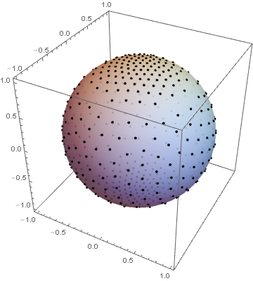
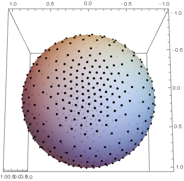
Figure 4. Two views of an approximation of $500$-point $(2,2,q_{2})$-energy minimizer $\omega_{\text{b}}$ from Example 3.2.

Again, let $A=\mathbb{S}^{2}\subset\mathbb{R}^{3},\ s=d=2$. Let us construct a sequence of discrete collections $\{\hat{\omega}_{N}\}_{N\geq 2}$ weak^∗ converging to the probability distribution with density proportional to

(3.2) $$\rho_{\text{b}}(x)=\begin{cases}10\cos(4\phi)+11,&0\leq\phi<\pi/4,\\ 1,&\pi/4\leq\phi<3\pi/4,\\ 10\cos(4\phi)+11,&3\pi/4\leq\phi,\end{cases}$$

where $\phi=\arccos(\langle x,\mathbf{e}_{z}\rangle)$. The external field with such a sequence of minimizers is provided by Theorem 2.3. Writing $\rho$ for the normalization of (3.2), $\rho(x):=\rho_{\text{b}}(x)/\int_{\mathbb{S}^{2}}|\rho_{\text{b}}|\,\mathrm{d}\mathcal{H}_{2}\approx\rho_{\text{b}}(x)/5.581722$, equation (2.5) gives the following external field:

$$q_{\text{b}}(x):=-2\pi\rho,$$

where we used again that $C_{2,2}=\pi$.

An approximate discrete minimizer of this $(2,2,q_{\text{b}})$-energy is shown in the Figure 4. Note how higher density of $\mu_{\mathbb{S}^{2}}^{q_{\text{b}}}$ (equivalently, larger values of $\rho$) causes charges to concentrate near the poles. Evaluating separation distance for the pictured configuration $\omega_{\text{b}}$ gives $\delta(\omega_{\text{b}})\approx 0.0777$, covering radius $\eta_{\text{b}}\approx 0.1681$. The mesh ratio of $\omega_{\text{b}}$ is therefore: $\gamma(\omega_{\text{b}},\mathbb{S}^{2})\approx 2.163$.

Example 3.3.

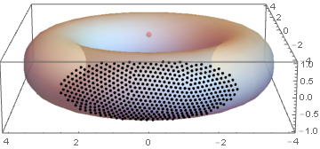
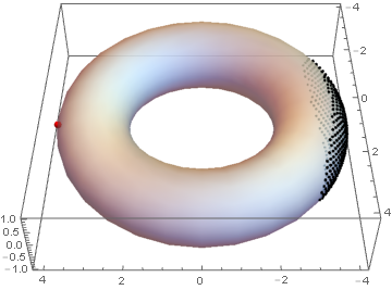
Figure 5. An approximation of $500$-point $(8,2,q_{\text{c}})$-energy minimizer $\omega_{c}$ from Example 3.3. The red dot marks position $(4,\ 0,\ 0)^{T}$, where the repelling external field $q_{\text{c}}$ is centered.

In this example the underlying set $A$ is a $2$-dimensional torus with inner radius $r_{i}=2$, outer radius $r_{o}=4$, centered at the origin. In particular, the point $(4,0,0)$ lies on the outer side of its surface. Consider the problem of minimizing $(8,2,q_{\text{c}})$-energy with the external field

$$q_{\text{c}}(x):=\|x-(4,\ 0,\ 0)^{T}\|^{-2}.$$

A resulting approximation of $500$-point minimizer $\omega_{\text{c}}$ is shown in Figure 5. Separation distance for this collection is $\delta(\omega_{\text{c}})\approx 0.125339$.

Example 3.4.

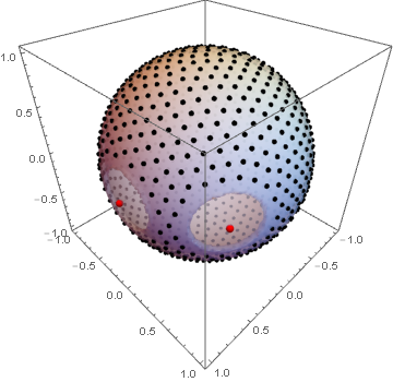
Figure 6. Two views of an approximation of $1000$-point energy minimizer from Example 3.4. The support of $\mu_{\mathbb{S}^{2}}^{q_{\text{d}}}$ is highlighted as are the positions of the fixed “repelling charges” that create the external field $q_{\text{d}}$.

Let us now consider an example of repelling field on the sphere $\mathbb{S}^{2}\subset\mathbb{R}^{3}$. Namely, we will minimize the $(4,2,q_{\text{d}})$-energy, where

$$q_{\text{d}}:=10^{-3}\left(\left\|x-(1,0,0)^{T}\right\|^{-4}+\left\|x-({0.5691,\ 0.8223,\ 0})^{T}\right\|^{-4}\right).$$

The second repelling charge is a randomly selected point in the first quadrant of $Oxy$ plane; factor $10^{-3}$ is used merely for convenience purposes.

An approximate 1000-point minimizer $\omega_{\text{d}}$ is shown in Figure 6. The shaded region marks the support of $\mu_{\mathbb{S}^{2}}^{q_{\text{d}}}$, obtained using formulas (2.1) with $C_{4,2}\approx 5.7834$ computed by the formula for its conjectured value (1.14). In other words, the shaded set is $\{x:q_{\text{d}}(x)\leq L_{1}(q_{\text{d}},\mathbb{S}^{2})\}\approx\{x:q_{\text{d}}(x)\leq 0.127\}$ (thus the complement of the support in the sphere consists of two circular-like regions). The separation distance of the pictured configuration is $\delta(\omega_{\text{d}})\approx 0.1015$.

Example 3.5.

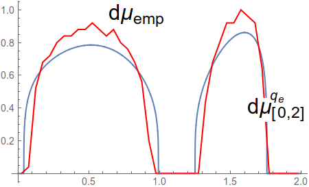
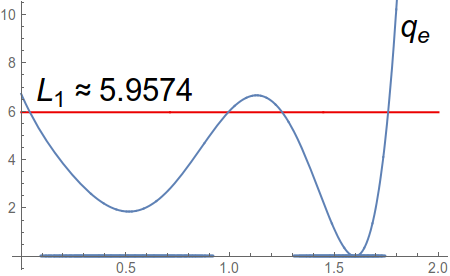
Figure 7. Left, empirical density $\,\mathrm{d}\mu_{\text{emp}}$ of $\omega_{\text{e}}$, an approximate $500$-point $(4,1,q_{\text{e}}(x))$-energy minimizer from Example 3.5 (red) overlaid with the graph of $\,\mathrm{d}\mu_{[0,2]}^{q_{\text{e}}}$ (blue); right, $\omega_{\text{e}}$ and the graph of external field $q_{\text{e}}$.

Finally, consider a $1$-dimensional example. We will minimize the $(4,1,q_{\text{e}})$-energy on the interval $[0,2]$, where

$$q_{\text{e}}(x):=(x-1.6)^{4}+40(x-0.2)^{4}(x-1.6)^{2}.$$

Substituting values of $s,d,C_{s,d}$ (the latter using formula (1.13)) into (2.1) gives that the weak^∗ limit of minimizers is the measure with density

$$\,\mathrm{d}\mu_{[0,2]}^{q_{\text{e}}}\approx\left(\frac{5.9574-q_{\text{e}}(\cdot)}{10.8232}\right)^{1/4}_{+}\,\mathrm{d}\mathcal{H}_{1}.$$

Figure 7 shows graphs of empirical density computed for $\omega_{\text{e}}$ and $\,\mathrm{d}\mu_{[0,2]}^{q_{\text{e}}}$, as well as the graph of $q_{\text{e}}$. Separation distance of the pictured configuration is $\delta(\omega_{\text{e}})\approx 0.0051$.

4. Proofs

For $s\geq d$, we denote by $\mathcal{R}_{s}^{d}$ the collection of all compact $d$-rectifiable sets $A\subset\mathbb{R}^{p}$ with $\mathcal{H}_{d}(A)>0$ and, in the case $s=d$, additionally require $A$ to be a subset of a $d$-dimensional $C^{1}$-manifold in $\mathbb{R}^{p}$. For $A\in\mathcal{R}_{s}^{d}$ and a suitable external field $q$, the values of $L_{1}$ and $S(q,A)$ are defined by (2.1) and (2.2), respectively. For real sequences $\{\zeta_{N}\}_{1}^{\infty}$, $\{\xi_{N}\}_{1}^{\infty}$ we shall use the notation $\zeta_{N}\sim\xi_{N},\ N\to\infty$ to mean $\zeta_{N}/\xi_{N}\to 1,\ N\to\infty$.

Observe that in the formula (1.1) the scaling factor $\tau_{s,d}(N)$ depends on $N$, the number of elements in $\omega_{N}$. We will occasionally need to evaluate the $(s,d,q)$-energy of a discrete $\omega\subset A$ with $\#\omega\neq N$ and the scaling factor $\tau_{s,d}(N)$, that is, the value of

(4.1) $$E^{q}_{s,d}(\omega,N):=E^{0}_{s,d}(\omega)+\frac{\tau_{s,d}(N)}{N}\,\sum_{x\in\omega}q(x),\quad s\geq d.$$

Throughout this section $\mathbb{N}$ stands for the set of positive integers. For $s\geq d$ we also define

$$\underline{g}^{q}_{s,d}(A):=\liminf_{N\to\infty}\frac{\mathcal{E}_{s,d}^{q}(A,N)}{\tau_{s,d}(N)},\qquad\overline{g}^{q}_{s,d}(A):=\limsup_{N\to\infty}\frac{\mathcal{E}_{s,d}^{q}(A,N)}{\tau_{s,d}(N)},$$

and if the limits coincide, the common value is denoted by

$$g^{q}_{s,d}(A)=\underline{g}^{q}_{s,d}(A)=\overline{g}^{q}_{s,d}(A).$$

Remark 4.1.

Note that for $s\geq d$ both the lower and upper asymptotic limits are finite if $q$ is finite-valued on a set of positive measure. Indeed, then there exists an $L_{*}$ such that $\mathcal{H}_{d}^{A}(\{x\in A:q(x)\leq L_{*}\})>0$, so the fact that $\underline{g}^{q}_{s,d}(A)$ and $\overline{g}^{q}_{s,d}(A)$ are finite follows from Theorem A and a simple observation: for any two functions $q_{1},\ q_{2}$ satisfying the hypotheses of Theorem 2.1, the inequality $q_{1}(x)\leq q_{2}(x),\ \forall x\in A,$ implies $\mathcal{E}^{q_{1}}_{s,d}(A,N)\leq\mathcal{E}^{q_{2}}_{s,d}(A,N)$. It suffices to put $q_{1}:=q,\ q_{2}(x)\equiv L_{*}$ and restrict the minimization problem to $\{x\in A:q(x)\leq L_{*}\}$.

Remark 4.2.

If $q$ is finite valued on a set of positive measure, then the constant $L_{1}$ in (2.1) is finite:

$$L_{1}\leq C_{s,d}\left(\mathcal{H}_{d}^{A}(\{x\in A:q(x)<L_{*}\})\right)^{-s/d}(1+s/d)+L_{*},$$

where $L_{*}$ is as in Remark 4.1.

Remark 4.3.

We will use in many computations that if a sequence $\{a_{N}\}_{N\in\mathcal{N}}$ with $a_{N}>0$ satisfies $\lim_{\mathcal{N}\ni N\to\infty}a_{N}/{N}=\alpha\geq 0$, then

(4.2) $$\lim_{\begin{subarray}{c}N\to\infty\\ N\in\mathcal{N}\end{subarray}}\frac{\tau_{s,d}\left(a_{N}\right)}{\tau_{s,d}(N)}=\alpha^{1+s/d}.$$

4.1. Proofs of the main theorems

We first establish a few lemmas that will be used in the proof of Theorem 2.1.

Lemma 4.4.

Let $u,v>0$ and $q_{0},q_{1}$ be real. Then the function

(4.3) $$F(t):=tq_{0}+(1-t)q_{1}+ut^{1+s/d}+v(1-t)^{1+s/d},\quad s\geq d,$$

has a unique minimum on $[0,1]$. If there is some $t_{*}$ in $(0,1)$ that satisfies

(4.4) $$\frac{q_{1}-q_{0}}{1+s/d}=ut_{*}^{s/d}-v(1-t_{*})^{s/d},$$

then the minimum occurs at $t_{*}$. Otherwise, the minimum occurs at $t_{*}\in\{0,1\}$ such that $q_{1-t_{*}}=\min\{q_{0},q_{1}\}$.

Proof..

As $F$ is strictly convex on $[0,1]$, it has a unique minimum in this interval. Differentiating yields $F^{\prime}(t)=q_{0}-q_{1}+(1+s/d)(ut^{s/d}-v(1-t)^{s/d})$. If there is a $t_{*}\in(0,1)$ satisfying (4.4), then $F^{\prime}(t_{*})=0$ and the minimum of $F$ occurs at the value $t_{*}$. Otherwise, $F$ is strictly monotone in $[0,1]$, and the minimium must occur at an endpoint. In fact, the minimum is at $t_{*}\in\{0,1\}$ such that $q_{1-t_{*}}=\min\{q_{0},q_{1}\}$. ∎

Lemma 4.5.

Let $\lambda$ be a finite Radon measure on the set $A\subset\mathbb{R}^{p}$ and $q:A\to\mathbb{R}$ be measurable with respect to $\lambda$. Then for every $\epsilon>0$ and $\lambda$-a.e. point $x\in\mathbb{R}^{p}$ there exists a positive number $R=R(x,\epsilon)$ such that

(4.5) $$\frac{\lambda\left[\{z\in A\cap B(x,r):|q(z)-q(x)|<\epsilon\}\right]}{\lambda[B(x,r)]}>1-\epsilon$$

for all $r<R$.

Proof..

Consider the following partition of set $A$:

(4.6) $$A=\bigcup_{m=1}^{\infty}\left\{(m-1)\epsilon\leq q(x)<m\epsilon\right\}=:\bigcup_{m=1}^{\infty}{A}_{m}.$$

By the Lebesgue-Besicovitch differentiation theorem (cf. [13, 1.7.1] or [21, Corollary 2.14]) (or Lebesgue’s density theorem in this case), for $\lambda$-a.e. point $x\in A_{m},\ m=1,2,\ldots,$

(4.7) $$\lim_{r\downarrow 0}\frac{\lambda[A_{m}\cap{B}(x,r)]}{\lambda[{B}(x,r)]}=1.$$

Therefore, (4.7) holds for $\lambda$-a.e. point $x\in A$. In particular, fix such a point $x\in A_{m}$. Because $(A_{m}\cap B(x,r))\subset\{z\in B(x,r):|q(z)-q(x)|<\epsilon\}$, equation (4.7) implies (4.5) for small enough $R$. ∎

Lemma 4.6.

Let $A\subset\mathbb{R}^{p}$ satisfy $A=\cup_{m=1}^{M}A_{m}$, where $A_{m}$ are sets from the class $\mathcal{R}_{s}^{d}$. Let also the function $q$ be defined and lower semi-continuous on $A$. Assume that a sequence of configurations $\omega_{n}\subset A$, $n\in\mathcal{N}$, is such that

1. $\omega_{n}=\bigcup_{m=1}^{M}\omega^{m}_{n}$ and $\omega^{m}_{n}\subset A_{m}$;

2. $\omega_{n}^{k}\cap\omega_{n}^{l}=\emptyset$ if $k\neq l$;

3. $\lim_{\mathcal{N}\ni n\to\infty}\#\omega^{m}_{n}/n=\alpha_{m},\ 1\leq m\leq M.$

Then

(4.8) $$\liminf_{\mathcal{N}\ni n\to\infty}\frac{E^{q}_{s,d}(\omega_{n},n)}{\tau_{s,d}(n)}\geq\sum_{m=1}^{M}\alpha_{m}^{1+s/d}\frac{C_{s,d}}{\mathcal{H}_{d}(A_{m})^{s/d}}+\sum_{m=1}^{M}\alpha_{m}\min_{x\in A_{m}}q(x).$$

Proof..

Observe that the minima on the right hand side of (4.8) are attained due to the lower semi-continuity of $q$. For the left hand side of (4.8) there holds

$$\liminf_{\mathcal{N}\ni n\to\infty}\frac{E^{q}_{s,d}(\omega_{n},n)}{\tau_{s,d}(n)}= \ \liminf_{\mathcal{N}\ni n\to\infty}\frac{1}{\tau_{s,d}(n)}\left(\sum_{\begin{subarray}{c}x\neq y\\ x,y\in\omega_{n}\end{subarray}}|x-y|^{-s}+\frac{\tau_{s,d}(n)}{n}\sum_{x\in\omega_{n}}q(x)\right)$$

$$\geq \ \liminf_{\mathcal{N}\ni n\to\infty}\frac{1}{\tau_{s,d}(n)}\sum_{m=1}^{M}\sum_{\begin{subarray}{c}x\neq y\\ x,y\in\omega^{m}_{n}\end{subarray}}|x-y|^{-s}+\liminf_{n\to\infty}\frac{1}{n}\sum_{m=1}^{M}\sum_{x\in\omega^{m}_{n}}q(x)$$

$$\geq \ \liminf_{\mathcal{N}\ni n\to\infty}\sum_{m=1}^{M}\frac{\tau_{s,d}(\#\omega^{m}_{n})}{\tau_{s,d}(n)}\frac{E^{0}_{s,d}(\omega^{m}_{n})}{\tau_{s,d}(\#\omega^{m}_{n})}+\liminf_{n\to\infty}\sum_{m=1}^{M}\frac{\#\omega^{m}_{n}}{n}\min_{x\in A_{m}}q(x)$$

$$\geq \ \sum_{m=1}^{M}\alpha_{m}^{1+s/d}\frac{C_{s,d}}{\mathcal{H}_{d}(A_{m})^{s/d}}+\sum_{m=1}^{M}\alpha_{m}\min_{x\in A_{m}}q(x),$$

where for the last inequality we used (4.2) and Theorem A. ∎

Remark 4.7.

Observe that the only assertion about $\#\omega_{n}$ we make is (3).

Corollary 4.8.

Let the assumptions of Lemma 4.6 be satisfied and suppose $q_{m},\ 1\leq m\leq M$, are numbers such that the closure of $Z_{m}:=\{x\in A_{m}:q(x)<q_{m}\}$ has $\mathcal{H}_{d}$-measure zero. Then

(4.9) $$\liminf_{\mathcal{N}\ni n\to\infty}\frac{E^{q}_{s,d}(\omega_{n},n)}{\tau_{s,d}(n)}\geq\sum_{m=1}^{M}\alpha_{m}^{1+s/d}\frac{C_{s,d}}{\mathcal{H}_{d}(A_{m})^{s/d}}+\sum_{m=1}^{M}\alpha_{m}q_{m}.$$

Proof..

Let $\mathcal{N}^{\prime}\subset\mathcal{N}$ be such that

$$\liminf_{\mathcal{N}\ni n\to\infty}\frac{E^{q}_{s,d}(\omega_{n},n)}{\tau_{s,d}(n)}=\lim_{\mathcal{N}^{\prime}\ni n\to\infty}\frac{E^{q}_{s,d}(\omega_{n},n)}{\tau_{s,d}(n)}.$$

Then

$$\lim_{\mathcal{N}^{\prime}\ni n\to\infty}\frac{E^{q}_{s,d}(\omega_{n},n)}{\tau_{s,d}(n)}\geq \sum_{m=1}^{M}\alpha_{m}^{1+s/d}\frac{C_{s,d}}{\mathcal{H}_{d}(A_{m})^{s/d}}+\lim_{\mathcal{N}^{\prime}\ni n\to\infty}\frac{1}{n}\sum_{m=1}^{M}\sum_{x\in\omega^{m}_{n}}q(x)$$

$$\geq \sum_{m=1}^{M}\alpha_{m}^{1+s/d}\frac{C_{s,d}}{\mathcal{H}_{d}(A_{m})^{s/d}}+\lim_{\mathcal{N}^{\prime}\ni n\to\infty}\frac{1}{n}\left(\sum_{m=1}^{M}\frac{\#(\omega_{n}^{m}\cap(A\setminus Z_{m}))}{n}\right)$$

$$= \sum_{m=1}^{M}\alpha_{m}^{1+s/d}\frac{C_{s,d}}{\mathcal{H}_{d}(A_{m})^{s/d}}+\sum_{m=1}^{M}\alpha_{m}q_{m}.$$

∎

Lemma 4.9.

Let the set $A$ be such that the assumptions of Theorem 2.1 hold. Assume that a sequence of $N$-point configurations $\{\omega_{N}\}_{N\geq 2}$ in $A$ satisfies

(4.10) $$\limsup_{\begin{subarray}{c}N\to\infty\\ N\in\mathcal{N}\end{subarray}}\frac{E^{q}_{s,d}(\omega_{N})}{\tau_{s,d}(N)}<+\infty$$

and

(4.11) $$\frac{1}{N}\sum_{x\in{\omega}_{N}}\delta_{x}\stackrel{{\scriptstyle*}}{{\longrightarrow}}\,\mathrm{d}\mu,\qquad\mathcal{N}\ni N\to\infty,$$

for some Borel probability measure $\mu$ on $A$. Then $\mu$ is $\mathcal{H}_{d}^{A}$-absolutely continuous.

Proof..

Indeed, otherwise let $E\subset A$ be a Borel set such that $\mathcal{H}_{d}(E)=0$ and $\mu(E)>0$. Since $\mu$ is inner regular as a Borel measure on a Radon space, [14, 434K(b)], without loss of generality $E$ is closed. For an $\epsilon>0$ pick $r>0$ such that $E_{r}:=\{x\in A:\mathrm{dist}(x,E)\leq r\}$ satisfies $\mathcal{H}_{d}(E_{r})<\epsilon$; observe that $E_{r}$ is closed. By the definition of weak^∗ convergence and Urysohn’s lemma, $\lim_{\mathcal{N}\ni N\to\infty}\frac{1}{N}\#\{x\in{\omega}_{N}:x\in E_{r}\}\geq\mu(E)$ (consider a positive continuous function equal 1 on $E$ and supported on $E_{r}$). Then according to Theorem A and the limit (4.2),

$$\liminf_{\begin{subarray}{c}N\to\infty\\ N\in\mathcal{N}\end{subarray}}\frac{E^{0}_{s,d}({\omega}_{N}\cap E_{r},N)}{\tau_{s,d}(N)} =\liminf_{\begin{subarray}{c}N\to\infty\\ N\in\mathcal{N}\end{subarray}}\frac{E^{0}_{s,d}({\omega}_{N}\cap E_{r},N)}{\tau_{s,d}(\#({\omega}_{N}\cap E_{r}))}\frac{\tau_{s,d}(\#({\omega}_{N}\cap E_{r}))}{\tau_{s,d}(N)}$$

$$\geq\frac{C_{s,d}}{\mathcal{H}_{d}(E_{r})^{s/d}}\mu(E)^{1+s/d}\geq\frac{C_{s,d}}{\epsilon^{s/d}}\mu(E)^{1+s/d}.$$

As $\epsilon$ was arbitrary, this contradicts (4.10). Thus $\mu$ must be $\mathcal{H}_{d}^{A}$-absolutely continuous. ∎

Lemma 4.10.

Let the assumptions of Theorem 2.1 be satisfied. Let also the sequence of $N$-point configurations $\{{\omega}_{N}\}_{N\in\mathcal{N}}$ be such that

(4.12) $$\lim_{\begin{subarray}{c}N\to\infty\\ N\in\mathcal{N}\end{subarray}}\frac{E^{q}_{s,d}({\omega}_{N})}{\tau_{s,d}(N)}=\underline{g}^{q}_{s,d}(A)$$

and

(4.13) $$\frac{1}{N}\sum_{x\in{\omega}_{N}}\delta_{x}\stackrel{{\scriptstyle*}}{{\longrightarrow}}\,\mathrm{d}{\mu},\qquad\mathcal{N}\ni N\to\infty.$$

Assume that $\{B_{m}\}_{m=1}^{M},\ M\geq 1,$ is a collection of closed pairwise disjoint balls such that $\mathcal{H}_{d}^{A}(B_{m})>0,\ \mathcal{H}_{d}^{A}(\partial B_{m})=0$ and ${\mathcal{H}_{d}^{A}\left(\{z\in B_{m}:q(z)\leq q_{m}\}\right)}\geq(1-\delta)\mathcal{H}_{d}^{A}(B_{m})$, $m=1,\ldots,M,$ for some positive $\delta<1$.

Then

(4.14) $$\lim_{\begin{subarray}{c}N\to\infty\\ N\in\mathcal{N}\end{subarray}}\frac{E^{q}_{s,d}({\omega}_{N}\cap\left(\cup_{m}B_{m}\right),N)}{\tau_{s,d}(N)}\leq\min\left\{\sum_{m=1}^{M}\frac{C_{s,d}\,\alpha_{m}^{1+s/d}}{((1-\delta)\mathcal{H}_{d}^{A}(B_{m}))^{s/d}}+q_{m}\alpha_{m}\right\},$$

where the minimum is taken over $\alpha_{m}\geq 0$ such that $\sum\alpha_{m}=\sum\mu(B_{m})$.

In particular, there exists a sequence $\{\omega_{N}^{0}\}_{N\in\mathcal{N}}$ for which (4.14) is an equality with $\omega_{N}^{0}$ in place of $\omega_{N}$.

Proof..

Fix an $\epsilon>0$ satisfying $\epsilon<1-\delta$. Consider the set $\{z\in B_{m}:q(z)\leq q_{m}\},\ m=1,\ldots,M$. By the inner regularity of measure $\mathcal{H}_{d}^{A}$, it has a closed subset $B^{\prime}_{m}$ contained in a ball concentric with $B_{i}$ of smaller radius, for which $\mathcal{H}_{d}^{A}(B^{\prime}_{m})>(1-\delta-\epsilon)\mathcal{H}_{d}^{A}(B_{m})$. Let a sequence of $N$-point configurations $\{\omega_{N}^{0}\}_{N\in\mathcal{N}}$ in $A$ be such that $\omega_{N}^{0}\cap(A\setminus\cup_{m}B_{m})=\omega_{N}\cap(A\setminus\cup_{m}B_{m})$, and such that for $1\leq m\leq M$, the collection ${\omega}_{N}^{0}\cap B_{m}$ is a minimizer of the $(s,d,0)$-energy in $B^{\prime}_{m}$ (in particular, is contained in it).

Equation (4.12) and Lemma 4.9 imply that $\mu(\partial B_{m})=0,\ 1\leq m\leq M$. Hence the weak^∗ convergence in (4.13) implies $\lim\#\{x\in\omega_{N}:x\in B_{m}\}/N\to\mu(B_{m})$ when $\mathcal{N}\ni N\to\infty$, [3, Theorem 2.1].

We will further assume that the following limits exist $\alpha_{m}:=\lim_{\mathcal{N}\ni N\to\infty}\#(\omega_{N}^{0}\cap B_{m})/N$, $1\leq m\leq M$. The assumptions on $\#(\omega_{N}^{0}\cap B_{m})$ mean that $\sum_{m}\alpha_{m}=\sum_{m}\mu(B_{m})$. Finally, we observe that by the construction of the sets $B_{m}^{\prime}$, there exists a positive $r$ such that $\mathrm{dist}(\cup_{m}B_{m}^{\prime},A\setminus\cup_{m}B_{m})\geq r$. Recall that

(4.15) $$E^{q}_{s,d}({\omega}_{N}^{0},N)=E^{q}_{s,d} \left({\omega}_{N}^{0}\cap(\cup_{m}B_{m}),N\right)+E^{q}_{s,d}\left({\omega}_{N}^{0}\cap(A\setminus\cup_{m}B_{m}),N\right)$$

$$+\sum_{\begin{subarray}{c}x,y\in\omega_{N}^{0},\\ x\in\cup_{m}B_{m},\\ y\in A\setminus\cup_{m}B_{m}\end{subarray}}|x-y|^{-s}.$$

Because $\omega_{N}^{0}\cap\cup_{m}B_{m}=\omega_{N}^{0}\cap\cup_{m}B^{\prime}_{m}$ and because of the lower bound $r$ for the distance between $\cup_{m}B^{\prime}_{m}$ and $A\setminus\cup_{m}B_{m}$, every term in the last sum is at most $r^{-s}$.

Using the previous equation and the definition of $\underline{g}^{q}_{s,d}(A)$, we have:

(4.16) $$0\leq \lim_{\begin{subarray}{c}N\to\infty\\ N\in\mathcal{N}\end{subarray}}\frac{E^{q}_{s,d}({\omega}_{N}^{0},N)}{\tau_{s,d}(N)}-\underline{g}^{q}_{s,d}(A)=\lim_{\begin{subarray}{c}N\to\infty\\ N\in\mathcal{N}\end{subarray}}\left(\frac{E^{q}_{s,d}({\omega}_{N}^{0})}{\tau_{s,d}(N)}-\frac{E^{q}_{s,d}({\omega}_{N})}{\tau_{s,d}(N)}\right)$$

$$\leq \lim_{\begin{subarray}{c}N\to\infty\\ N\in\mathcal{N}\end{subarray}}\frac{E^{q}_{s,d}({\omega}_{N}^{0}\cap\left(\cup_{m}B_{m}\right),N)}{\tau_{s,d}(N)}-\lim_{\begin{subarray}{c}N\to\infty\\ N\in\mathcal{N}\end{subarray}}\frac{E^{q}_{s,d}({\omega}_{N}\cap\left(\cup_{m}B_{m}\right),N)}{\tau_{s,d}(N)}$$

$$+\lim_{\begin{subarray}{c}N\to\infty\\ N\in\mathcal{N}\end{subarray}}\frac{N^{2}}{\tau_{s,d}(N)}r^{-s}.$$

Since $\lim_{\begin{subarray}{c}N\to\infty\\ N\in\mathcal{N}\end{subarray}}{N^{2}}r^{-s}/{\tau_{s,d}(N)}=0$, there holds

(4.17) $$\lim_{\begin{subarray}{c}N\to\infty\\ N\in\mathcal{N}\end{subarray}}\frac{E^{q}_{s,d}({\omega}_{N}\cap\left(\cup_{m}B_{m}\right),N)}{\tau_{s,d}(N)}\leq\lim_{\begin{subarray}{c}N\to\infty\\ N\in\mathcal{N}\end{subarray}}\frac{E^{q}_{s,d}({\omega}_{N}^{0}\cap\left(\cup_{m}B_{m}\right),N)}{\tau_{s,d}(N)}.$$

From equation (4.12) and Lemma 4.9 follows that $\mu(\partial B_{m})=0,\ 1\leq m\leq M$. Hence the weak^∗ convergence in (4.13) implies $\lim\#\{x\in\omega_{N}:x\in B_{m}\}/N\to\mu(B_{m})$ when $\mathcal{N}\ni N\to\infty$, [3, Theorem 2.1]. The construction of the sequence $\{\omega_{N}^{0}\}_{N\in\mathcal{N}}$ and the limit (4.2) therefore imply

(4.18) $$\lim_{\begin{subarray}{c}N\to\infty\\ N\in\mathcal{N}\end{subarray}}\frac{E^{q}_{s,d}({\omega}_{N}^{0}\cap\left(\cup_{m}B_{m}\right),N)}{\tau_{s,d}(N)}\leq\sum_{m=1}^{M}\left(\frac{C_{s,d}\,\alpha_{m}^{1+s/d}}{((1-\delta-\epsilon)\mathcal{H}_{d}^{A}(B_{m}))^{s/d}}+q_{m}\alpha_{m}\right).$$

We have so far only imposed the conditions that $\alpha_{1},\ldots,\alpha_{M}$ are nonnegative and sum to $\sum_{m}\mu(B_{m})$. Taking $\epsilon\to 0+$ and minimizing over such $\alpha_{m}$ in (4.18) gives (4.14). ∎

We first prove Theorem 2.1 for the case that $q$ is a suitable simple function. The general case then follows by approximating an arbitrary lower semi-continuous $q$ with such functions.

Lemma 4.11.

Let $A\subset\mathbb{R}^{p}$ be a set from $\mathcal{R}_{s}^{d}$, and $B_{m},\,1\leq m\leq M$, be a collection of pairwise disjoint closed balls such that $\mathcal{H}_{d}^{A}(B_{m})>0$ and $\mathcal{H}_{d}^{A}(A\cap\partial B_{m})=0,\ 1\leq m\leq M$. Assume also $q$ is a lower semi-continuous function and for $D:=\overline{A\setminus\cup_{m}B_{m}}$,

(4.19) $$q(x)=\begin{cases}q_{0},&\mathcal{H}_{d}^{A}\text{-a.e. }x\in D,\\ q_{m},&\mathcal{H}_{d}^{A}\text{-a.e. }x\in B_{m},\quad 1\leq m\leq M,\end{cases}$$

for positive $q_{m},\ 0\leq m\leq M$.

Then equation (2.2) holds for the set $A$ and function $q$.

Proof..

For convenience, let $A_{0}:=D$, $A_{m}:=B_{m},\ 1\leq m\leq M$, in this proof. We will first verify that for some positive $\{\hat{\alpha}_{m}\}_{m=0}^{M}$ that add up to one,

(4.20) $$\lim\limits_{N\to\infty}\frac{\mathcal{E}_{s,d}^{q}(A,N)}{\tau_{s,d}(N)}=\sum_{m=0}^{M}\left(\frac{C_{s,d}\,\hat{\alpha}_{m}^{1+s/d}}{\mathcal{H}_{d}^{A}(A_{m})^{s/d}}+q_{m}\hat{\alpha}_{m}\right),$$

where the values of $\hat{\alpha}_{m},\ 0\leq m\leq M$ are such that

(4.21) $$(\hat{\alpha}_{0},\ldots,\hat{\alpha}_{M}):=\underset{\begin{subarray}{c}\alpha_{m}\geq 0,\\ \sum\alpha_{m}=1\end{subarray}}{\arg\min}\sum_{m=0}^{M}\left(\frac{C_{s,d}\,\alpha_{m}^{1+s/d}}{\mathcal{H}_{d}^{A}(A_{m})^{s/d}}+q_{m}\alpha_{m}\right).$$

(i). Due to the weak^∗ compactness of the set $A$, Corollary 4.8 implies

(4.22) $$\underline{g}^{q}_{s,d}(A)\geq\min_{\begin{subarray}{c}\alpha_{m}\geq 0,\\ \sum\alpha_{m}=1\end{subarray}}\sum_{m=0}^{M}\left(\frac{C_{s,d}\,\alpha_{m}^{1+s/d}}{\mathcal{H}_{d}^{A}(A_{m})^{s/d}}+q_{m}\alpha_{m}\right).$$

Let a closed $D^{\prime}\subset D$ satisfy $q(x)\equiv q_{0},\ x\in D^{\prime}$ and $\mathcal{H}_{d}^{A}(D^{\prime})>(1-\epsilon)\mathcal{H}_{d}^{A}(D)$. By the same argument as in the proof of Lemma 4.10, for a fixed $\epsilon>0$ we construct a sequence of $N$-element sets $\{\omega_{N}^{0}\}_{N\in\mathcal{N}}$ such that the subsets $\omega_{N}^{0}\cap D$ and $\omega_{N}^{0}\cap B_{m},\ 1\leq m\leq M$ are $(s,d,0)$-energy minimizing in $D^{\prime}$ and $B_{m}^{\prime}$ respectively. Recall that $B_{m}^{\prime}$ are closed subsets of $A\cap B_{m}$ satisfying $\mathcal{H}_{d}^{A}(B_{m}^{\prime})>(1-\epsilon)\mathcal{H}_{d}^{A}(B_{m})$ and $\mathrm{dist}(\cup_{m}B_{m}^{\prime},D)>0$. As in Lemma 4.10, we construct $\{\omega_{N}^{0}\}_{N\geq 1}$ so that the following limits exist and are finite $\alpha_{0}:=\lim_{\mathcal{N}\ni N\to\infty}\#(\omega_{N}^{0}\cap D^{\prime})/N$ and $\alpha_{m}:=\lim_{\mathcal{N}\ni N\to\infty}\#(\omega_{N}^{0}\cap B_{m})/N$, $1\leq m\leq M$. Since $\mathcal{E}_{s,d}^{q}(A,N)\leq E^{q}_{s,d}({\omega}_{N}^{0},N)$, equation (4.15) implies

(4.23) $$\overline{g}^{q}_{s,d}(A)\leq\lim_{N\to\infty}\frac{E^{q}_{s,d}({\omega}_{N}^{0},N)}{\tau_{s,d}(N)}=\sum_{m=0}^{M}\left(\frac{C_{s,d}\,\alpha_{m}^{1+s/d}}{((1-\epsilon)\mathcal{H}_{d}^{A}(A_{m}))^{s/d}}+q_{m}\alpha_{m}\right).$$

This gives (4.20) after taking $\epsilon\to 0+$.

(ii). Fix an $A_{m}$ with strictly positive $\hat{\alpha}_{m}$, say, $A_{0}$ and assume $q_{0}\leq q_{m}$ for definiteness. Pick any of the remaining sets $A_{k},\ 1\leq k\leq M$ and denote $\beta=\beta(k):=\alpha_{0}+\alpha_{k}$. Consider the terms on the right hand side of (4.21) that contain either $\alpha_{0}$ or $\alpha_{k}$:

(4.24) $$\bar{F}({\alpha}_{1},{\alpha}_{k}):=\sum_{m=0,k}\left(\frac{C_{s,d}\,{\alpha}_{m}^{1+s/d}}{\mathcal{H}_{d}^{A}(A_{m})^{s/d}}+q_{m}{\alpha}_{m}\right).$$

Now choose the coefficients of the function $F(t)$ in Lemma 4.4 so that

(4.25) $$F(t)=\ t^{1+s/d}\frac{C_{s,d}}{\mathcal{H}_{d}^{A}(A_{0})^{s/d}}+t\frac{q_{0}}{\beta^{s/d}}+(1-t)^{1+s/d}\frac{C_{s,d}}{\mathcal{H}_{d}^{A}(A_{k})^{s/d}}+(1-t)\frac{q_{k}}{\beta^{s/d}},$$

then $\beta^{1+s/d}F(\alpha_{0}/\beta)=\bar{F}({\alpha}_{0},{\alpha}_{k})$. Because of (4.21), it must be that $\hat{\alpha}_{0}/\beta$ is the value $\hat{t}\in(0,1]$ for which the minimum of $F(t)$ is attained. According to Lemma 4.4, either $\hat{t}=1$, or

(4.26) $$\frac{q_{k}-q_{0}}{C_{s,d}(1+s/d)}=\left(\frac{\hat{\alpha}_{0}}{\mathcal{H}_{d}^{A}(A_{0})}\right)^{s/d}-\left(\frac{\hat{\alpha}_{k}}{\mathcal{H}_{d}^{A}(A_{k})}\right)^{s/d}.$$

Equation (4.26) thus applies to any pair of sets in $A_{0},\ldots,A_{M}$ provided both the corresponding $\hat{\alpha}_{m}$’s is positive. Also, if $\hat{\alpha}_{k}>0$, then $q_{k}<q_{l}$ for every $l$ such that $\hat{\alpha}_{l}=0$. To summarize, for some $L_{1}$ there holds

(4.27) $$\left(\frac{\hat{\alpha}_{m}}{\mathcal{H}_{d}^{A}(A_{m})}\right)^{s/d}=\left(\frac{L_{1}-q_{m}}{C_{s,d}(1+s/d)}\right)_{+},\qquad 0\leq m\leq M.$$

It follows from $\sum_{m}\hat{\alpha}_{m}=1$ that the first of equations (2.1) is satisfied for this $L_{1}$.

Finally, we can evaluate the right hand side of (4.20):

$$\lim\limits_{N\to\infty}\frac{\mathcal{E}_{s,d}^{q}(A,N)}{\tau_{s,d}(N)}=\sum_{m=0}^{M}\left(\hat{\alpha}_{m}\left(\frac{L_{1}-q_{m}}{1+s/d}\right)_{+}+q_{m}\hat{\alpha}_{m}\right)=\sum_{m=0}^{M}\hat{\alpha}_{m}\frac{L_{1}+sq_{m}/d}{1+s/d},$$

where in the last equality we used $\hat{\alpha}_{m}=0\iff(L_{1}-q_{m})_{+}=0$. This implies (2.2) because from (4.27), $\hat{\alpha}_{0}=\mu^{q}_{A}(D)$ and $\hat{\alpha}_{m}=\mu^{q}_{A}(A_{m}),\ 1\leq m\leq M$, for the $\mu^{q}_{A}$ defined in (2.1). ∎

Proof of Theorem 2.1..

Note that as $q$ is lower semi-continuous on the compact set $A$, it is bounded below there, so we may assume without loss of generality $q$ is positive.

(i). Let $A\in\mathcal{R}_{s}^{d}$ and let $0\leq q<C$ for a positive constant $C$. We will further use that the restriction $\mathcal{H}_{d}^{A}$ is a Radon measure on $\mathbb{R}^{p}$. Namely, [21, Theorem 7.5] implies it is locally finite because $A$ is the Lipschitz image of a compact set in $\mathbb{R}^{d}$. It is also Borel regular as a restriction of Hausdorff measure, see [21, Theorem 4.2]. Then by [21, Corollary 1.11], $\mathcal{H}_{d}^{A}$ is a Radon measure.

Fix from now on a number $0<\epsilon<1/4$. Apply Lemma 4.5 to the measure $\mathcal{H}_{d}^{A}$ and function $q$, denote the set of $x\in A$ for which there exists an $R(x,\epsilon)$ as described in the Lemma by $A^{\prime}$, and consider covering of $A^{\prime}$ by the collection of closed balls $\{{B}(x,r):x\in A^{\prime},\ 0<r<R(x,\epsilon)\}$. Choose for each $x\in A^{\prime}$ a sequence of radii $r_{x,k}\to 0,\ k\to\infty,\ k\in\mathbb{N},$ for which

(4.28) $$\frac{\mathcal{H}_{d}^{A}\left[\{z\in B(x,r_{x,k}):|q(z)-q(x)|<\epsilon\}\right]}{\mathcal{H}_{d}^{A}[B(x,r_{x,k})]}>1-\epsilon$$

and also $y\in A\cap{B}(x,r_{x,k})\implies q(y)>q(x)-\epsilon$. The latter is possible due to the lower semicontinuity of $q$.

Let $\{{B}(x,r_{x,k})\}$ be a Vitali cover of $A^{\prime}$, so one can apply the version of Vitali’s covering theorem for Radon measures [21, Theorem 2.8] to produce a (at most) countable subcollection of pairwise disjoint $\{B_{j}:={B}(x_{j},r_{j}):j\geq 1\}$ for which $\mathcal{H}_{d}\left(A^{\prime}\;{\setminus}\;\cup_{j\geq 1}B_{j}\right)=0$. Using $\mathcal{H}_{d}(A)<\infty$, $\{B_{j}\}_{j\geq 1}$ can be chosen so that $\mathcal{H}_{d}(A\cap\partial B_{j})=0,\ j=1,2,\ldots$ (there are uncountable many options for the value of $r_{j}$, at most countably many of them positive). Since $\mathcal{H}_{d}(A\setminus A^{\prime})=0$, we can fix a $J\in\mathbb{N}$ such that $\mathcal{H}_{d}\left(A\setminus\cup_{j=1}^{J}B_{j}\right)<\epsilon.$ Let $D:=\overline{A\setminus\cup_{j=1}^{\,J}B_{j}}$. As $\mathcal{H}_{d}^{A}(\partial B_{j})=0,\ 1\leq j\leq J$, there holds $\mathcal{H}_{d}^{A}(D)<\epsilon$.

Define the two simple functions $\overline{q}_{\epsilon},\ \underline{q}_{\epsilon}$ to be constant on each $B_{j},\ 1\leq j\leq J$:

(4.29) $$\begin{split}\overline{q}_{\epsilon}(x)&:=\begin{cases}q(x_{j})+\epsilon,&x\in B_{j},\\ C,&x\in D\setminus\bigcup_{j}B_{j}.\end{cases}\\ \underline{q}_{\epsilon}(x)&:=\begin{cases}\max(0,q(x_{j})-\epsilon),&x\in B_{j}\setminus D,\\ 0,&x\in D.\end{cases}\end{split}$$

Such $\underline{q}_{\epsilon},\ \overline{q}_{\epsilon}$ are lower semi-continuous on $A$. Lemma 4.11 gives equation (2.2) applied to $\underline{q}_{\epsilon}$ and $\overline{q}_{\epsilon}$ on $A$. Let $B_{j}^{\prime}:=\{z\in A\cap B_{j}:|q(z)-q(x_{j})|<\epsilon\}$. Then,

(4.30) $$q(x_{j})-\epsilon\leq\underline{q}_{\epsilon}(x)\leq q(x)\leq\overline{q}_{\epsilon}(X)=q(x_{j})_{\epsilon},\quad x\in B_{j}^{\prime}.$$

In view of (4.28) for $B_{j}^{\prime}$ and $\mathcal{H}_{d}^{A}(D)<\epsilon$, (4.30) implies that both $\underline{q}_{\epsilon}$ and $\overline{q}_{\epsilon}$ converge $\mathcal{H}_{d}^{A}$-a.e. to $q$ as $\epsilon\to 0+$. Since both are bounded by $C+1$, the dominated convergence theorem is applicable, and

(4.31) $$\lim_{\epsilon\to 0}S(\underline{q}_{\epsilon},A)=\lim_{\epsilon\to 0}S(\overline{q}_{\epsilon},A)=S(q,A).$$

We now estimate $\lim_{N\to\infty}{\mathcal{E}_{s,d}^{q}(A,N)}/{\tau_{s,d}(N)}$ in terms of $\lim_{N\to\infty}{\mathcal{E}^{\underline{q}_{\epsilon}}_{s,d}(A,N)}/{\tau_{s,d}(N)}$ and $\lim_{N\to\infty}{\mathcal{E}^{\overline{q}_{\epsilon}}_{s,d}(A,N)}/{\tau_{s,d}(N)}$. Firstly, by construction $q(x)\geq\underline{q}_{\epsilon}(x),\ x\in A$, which gives

(4.32) $$\mathcal{E}_{s,d}^{q}(A,N)\geq\mathcal{E}^{\underline{q}_{\epsilon}}_{s,d}(A,N).$$

On the other hand,

(4.33) $$\mathcal{E}_{s,d}^{q}(A,N)\leq\mathcal{E}_{s,d}^{q}(D\cup\bigcup_{j}B_{j}^{\prime},N)\leq\mathcal{E}^{\overline{q}}_{s,d}(D\cup\bigcup_{j}B_{j}^{\prime},N)\leq\frac{\tau_{s,d}(N)}{(1-\epsilon)^{s/d}}S(\overline{q}_{\epsilon},A),$$

where the last inequality follows from (4.28) and (4.20). This proves (2.2).

(ii). It remains to prove equation (2.4) for a sequence $\{{\omega}_{N}\}_{N\geq 2}$ satisfying (2.3). Since the probability measures on $A$ are weak^∗ compact, one can pick a subsequence $\{\hat{\omega}_{N}\}_{N\in\mathcal{N}}\subset\{\omega_{N}\}_{N\geq 2}$ for which the corresponding normalized counting measures have a weak^∗ limit:

$$\frac{1}{N}\sum_{x\in\hat{\omega}_{N}}\delta_{x}\stackrel{{\scriptstyle*}}{{\longrightarrow}}\mu,\qquad\mathcal{N}\ni N\to\infty.$$

Then $\mu$ is $\mathcal{H}_{d}^{A}$-absolutely continuous by the Lemma 4.9. Set $\rho(x):=\frac{\,\mathrm{d}\mu}{\,\mathrm{d}\mathcal{H}_{d}^{A}}(x)$.

Since the integral $\int_{A}\rho\,\mathrm{d}\mathcal{H}_{d}^{A}=1$ is finite, at $\mathcal{H}_{d}^{A}$-a.e. point $x$ of $A$ there holds

(4.34) $$\lim_{r\to 0}\frac{1}{\mathcal{H}_{d}^{A}(B(x,r))}\int_{B(x,r)}\rho\,\mathrm{d}\mathcal{H}_{d}^{A}=\rho(x).$$

Fix two distinct points $x_{1},\ x_{2}$ for which both (4.5) for measure $\mathcal{H}_{d}^{A}$ and (4.34) hold. Then for an arbitrary fixed $0<\epsilon<\min(1/2,\rho(x_{1}),\rho(x_{2}),q(x_{1}),q(x_{2}))$ there exist closed disjoint balls $B_{1}:=B(x_{1},r_{1}),\ B_{2}:=B(x_{2},r_{2})$ centered around $x_{1},\ x_{2}$ such that equations

(4.35) $$\frac{\mathcal{H}_{d}^{A}\left[\{z\in A\cap B_{m}:|q(z)-q(x_{m})|<\epsilon\}\right]}{\mathcal{H}_{d}^{A}[B_{m}]}>1-\epsilon,\qquad m=1,2,$$

(4.36) $$\int_{B_{m}}\left|\rho(z)-\rho(x_{m})\right|\,\mathrm{d}\mathcal{H}_{d}^{A}(z)<\epsilon\mathcal{H}_{d}^{A}(B_{m}),\qquad m=1,2,$$

hold for all closed balls concentric with $B_{m}$ of radius at most $r_{m}$. Without loss of generality we will also require $\mathcal{H}_{d}^{A}(\partial B_{1})=\mathcal{H}_{d}^{A}(\partial B_{2})=0$ and that $q(x)\geq q(x_{m})-\epsilon$ for all $x\in B_{m},\ m=1,2$ (which can be assumed by lower semi-continuity). Let $q_{m}:=q(x_{m}),\ m=1,2$; let also $q_{1}\leq q_{2}$.

Due to $\mu$ being absolutely continuous with respect to $\mathcal{H}_{d}^{A}$, the assumption $\mathcal{H}_{d}^{A}(\partial B_{m})=0,\ m=1,2$, and the limit (4.2), Lemma 4.6 implies

(4.37) $$\lim_{\begin{subarray}{c}N\to\infty\\ N\in\mathcal{N}\end{subarray}}\frac{E^{q}_{s,d}(\hat{\omega}_{N}\cap(B_{1}\cup B_{2}),N)}{\tau_{s,d}(N)}\geq\sum_{m=1,2}\left(\frac{C_{s,d}\,\mu(B_{m})^{1+s/d}}{\mathcal{H}_{d}^{A}(B_{m})^{s/d}}+\mu(B_{m})(q_{m}-\epsilon)\right).$$

On the other hand, from Lemma 4.10:

(4.38) $$\lim_{\begin{subarray}{c}N\to\infty\\ N\in\mathcal{N}\end{subarray}}\frac{E^{q}_{s,d}(\hat{\omega}_{N}\cap(B_{1}\cup B_{2}),N)}{\tau_{s,d}(N)}\leq\min\left\{\sum_{m=1,2}\frac{C_{s,d}\,\alpha_{m}^{1+s/d}}{((1-\epsilon)\mathcal{H}_{d}^{A}(B_{m}))^{s/d}}+(q_{m}+\epsilon)\alpha_{m}\right\}$$

with minimum taken over positive $\alpha_{1},\ \alpha_{2}$ satisfying $\alpha_{1}+\alpha_{2}=\mu(B_{1})+\mu(B_{2})$. If we denote

(4.39) $$(\hat{\alpha}_{1},\hat{\alpha}_{2}):=\arg\min\Bigg{\{}\sum_{m=1,2}\bigg{(}\frac{C_{s,d}\,\alpha_{m}^{1+s/d}}{((1-\epsilon)\mathcal{H}_{d}^{A}(B_{m}))^{s/d}} +(q_{m}+\epsilon)\alpha_{m}\Bigg{)}$$

$$\boldsymbol{:}\alpha_{1}+\alpha_{2}=\mu(B_{1})+\mu(B_{2})\Bigg{\}},$$

and argue as in the proof of Lemma 4.11, we obtain, similarly to (4.26), that $(\hat{\alpha}_{1},\hat{\alpha}_{2})$ satisfy

(4.40) $$\frac{q_{2}-q_{1}}{C_{s,d}(1+s/d)}=\left(\frac{\hat{\alpha}_{1}}{(1-\epsilon)\mathcal{H}_{d}^{A}(B_{1})}\right)^{s/d}-\left(\frac{\hat{\alpha}_{2}}{(1-\epsilon)\mathcal{H}_{d}^{A}(B_{2})}\right)^{s/d}.$$

Inequalities (4.37)–(4.38) and the definition of $(\hat{\alpha}_{1},\hat{\alpha}_{2})$ give:

(4.41) $$\sum_{m=1,2}\left(\frac{C_{s,d}\,\mu(B_{m})^{1+s/d}}{\mathcal{H}_{d}^{A}(B_{m})^{s/d}}+\mu(B_{m})(q_{m}-\epsilon)\right)$$

$$\leq \sum_{m=1,2}\left(\frac{C_{s,d}\,\hat{\alpha}_{m}^{1+s/d}}{((1-\epsilon)\mathcal{H}_{d}^{A}(B_{m}))^{s/d}}+\hat{\alpha}_{m}(q_{m}+\epsilon)\right)$$

$$\leq \sum_{m=1,2}\left(\frac{C_{s,d}\,\mu(B_{m})^{1+s/d}}{((1-\epsilon)\mathcal{H}_{d}^{A}(B_{m}))^{s/d}}+\mu(B_{m})(q_{m}+\epsilon)\right).$$

Observe that if in the above construction we fix the ball $B_{1}$ and allow $r_{2}\to 0$, the first term on the right hand side of (4.40) is bounded, so the ratio $\hat{\alpha}_{2}/\mathcal{H}_{d}^{A}(B_{2})$ is bounded as well, say, $\hat{\alpha}_{2}/\mathcal{H}_{d}^{A}(B_{2})\leq R_{2}$. Let also $r_{2}$ be such that $\mathcal{H}_{d}^{A}(B_{2})/\mathcal{H}_{d}^{A}(B_{1})<\epsilon$ and $\hat{\alpha}_{2}/\mathcal{H}_{d}^{A}(B_{1})<\epsilon$. Due to equation (4.36), there holds $|\mu(B_{m})/\mathcal{H}_{d}^{A}(B_{m})-\rho(x_{m})|<\epsilon,\ m=1,2$. Dividing (4.41) through by $\mathcal{H}_{d}^{A}(B_{1})$ for such a choice of $r_{2}$ gives:

(4.42) $$C_{s,d}(\rho(x_{1})-\epsilon)^{1+s/d}+(\rho(x_{1})-\epsilon)(q_{1}-\epsilon)$$

$$\boldsymbol{\leq} \frac{C_{s,d}}{(1-\epsilon)^{s/d}}\left(\frac{\hat{\alpha}_{1}}{\mathcal{H}_{d}^{A}(B_{1})}\right)^{1+s/d}+\left(\frac{\hat{\alpha}_{1}}{\mathcal{H}_{d}^{A}(B_{1})}\right)(q_{1}+\epsilon)$$

$$\qquad+\left(\frac{\hat{\alpha}_{2}}{\mathcal{H}_{d}^{A}(B_{1})}\right)\frac{C_{s,d}}{(1-\epsilon)^{s/d}}\left(\frac{\hat{\alpha}_{2}}{\mathcal{H}_{d}^{A}(B_{2})}\right)^{s/d}+\left(\frac{\hat{\alpha}_{2}}{\mathcal{H}_{d}^{A}(B_{1})}\right)(q_{2}+\epsilon)$$

$$\boldsymbol{\leq} \frac{C_{s,d}}{(1-\epsilon)^{s/d}}{(\rho(x_{1})+\epsilon)^{1+s/d}}+(\rho(x_{1})+\epsilon)(q_{1}+\epsilon)$$

$$\qquad+\epsilon\left(\frac{C_{s,d}}{(1-\epsilon)^{s/d}}{(\rho(x_{2})+\epsilon)^{1+s/d}}+(\rho(x_{2})+\epsilon)(q_{2}+\epsilon)\right),$$

Finally, because $\epsilon>0$ was arbitrary and the function $C_{s,d}t^{1+s/d}+q(x_{1})t,\ t\geq 0$ is monotone, inequalities (4.42) yield by the above discussion

(4.43) $$\rho(x_{1})=\lim_{r_{1}\to 0}\frac{\hat{\alpha}_{1}}{\mathcal{H}_{d}^{A}(B_{1})}.$$

We could similarly fix the ball $B_{2}$ first and ensure $\mathcal{H}_{d}^{A}(B_{1})/\mathcal{H}_{d}^{A}(B_{2})<\epsilon$, taking $r_{2}\to 0$ afterwards, thus also

(4.44) $$\rho(x_{2})=\lim_{r_{2}\to 0}\frac{\hat{\alpha}_{2}}{\mathcal{H}_{d}^{A}(B_{2})}.$$

In conjunction with (4.40) the last two equations give

(4.45) $$\frac{q_{2}-q_{1}}{C_{s,d}(1+s/d)}=\rho(x_{1})^{s/d}-\rho(x_{2})^{s/d}$$

for $\mathcal{H}_{d}^{A}\times\mathcal{H}_{d}^{A}$-a.e. pair $(x_{1},x_{2})\in A\times A$. Due to the normalization property $\int_{A}\rho(x)\,\mathrm{d}\mathcal{H}_{d}^{A}=1$ and the definition of $L_{1}$ in (2.1),

(4.46) $$\rho(x)=\left(\frac{L_{1}-q(x)}{C_{s,d}(1+s/d)}\right)^{d/s}_{+}\qquad\mathcal{H}_{d}^{A}\text{-a.e.}$$

which coincides with the density in formula (2.4).

(iii). Finally, we turn to the case when the function $q$ need not be bounded above. Consider

$$q_{\scalebox{0.6}{$C$}}(x):=\begin{cases}q(x),&q(x)\leq C,\\ C,\ &\text{otherwise}.\end{cases}$$

Recall that $A(C)=\{x\in A:q(x)\leq C\}$ is a $d$-rectifiable set as a closed subset of $A$. The Theorem 2.1 is therefore applicable to each function $q_{\scalebox{0.6}{$C$}}$ if seen as defined on $A(C)$. By Remark 4.2, the value of $L_{1}$ is finite. For all $C\geq L_{1}$,

(4.47) $$\operatorname{supp}(\mu_{A}^{q_{\scalebox{0.6}{$C$}}})\cap\{x:q(x)>C\}=\emptyset.$$

Inequality $q_{\scalebox{0.6}{$C$}}(x)\leq q(x)$ for all $x\in A$ implies

$$\mathcal{E}^{q_{\scalebox{0.6}{$C$}}}_{s,d}(A,N)\leq\mathcal{E}_{s,d}^{q}(A,N),\quad N\geq 2,$$

so $S(q_{\scalebox{0.6}{$C$}},A)\leq\underline{g}^{q}_{s,d}(A)$. On the other hand, due to set inclusion,

$$\underline{g}^{q}_{s,d}(A)\leq\overline{g}^{q}_{s,d}(A)\leq\overline{g}^{q}_{s,d}(A(C))=S(q_{\scalebox{0.6}{$C$}},A(C))=S(q_{\scalebox{0.6}{$C$}},A),$$

where the last two equalities follow from Theorem 2.1 applied to the function $q_{\scalebox{0.6}{$C$}}$ and sets $A(C)$ and $A$ respectively, and equation (4.47). To summarize, $\underline{g}^{q}_{s,d}(A)=\overline{g}^{q}_{s,d}(A)=S(q,A)$.

Let now $\{{\omega}_{N}\}_{N\geq 2}$ be a sequence satisfying (2.3). Fix a $C>L_{1}$. Because $q_{\scalebox{0.6}{$C$}}(x)\leq q(x)\$ for all $x\in A$ and $S(q,A)=S(q_{\scalebox{0.6}{$C$}},A)$, the sequence $\{{\omega}_{N}\}_{N\geq 2}$ is also asymptotically $(s,d,q_{\scalebox{0.6}{$C$}})$-energy minimizing. Then by Theorem 2.1 this sequence converges weak^∗ to $\,\mathrm{d}\mu_{A}^{q_{\scalebox{0.6}{$C$}}}$, and it remains to observe that for $C>L_{1}$ it holds $\,\mathrm{d}\mu_{A}^{q_{\scalebox{0.6}{$C$}}}=\,\mathrm{d}\mu_{A}^{q}$, where the two measures are defined in equation (2.1). ∎

Proof of Theorem 2.3..

The desired result is an immediate application of Theorem 2.1 since using equation (2.1) for the external field from (2.5) gives $L_{1}=0$, so the asymptotic distribution is indeed (2.6). ∎

Proof of Proposition 2.5..

We have

$$q^{\prime}(x)=(1+\Delta)q(x).$$

According to (2.1), the equation

(4.48) $$\int\left(\frac{l-q^{\prime}(x)}{M_{s,d}}\right)^{d/s}_{+}\,\mathrm{d}\mathcal{H}_{d}^{A}(x)=1$$

for variable $l$ has the unique solution $l=L^{\prime}_{1}$. Using (2.5), it can be rewritten as

(4.49) $$\int\left(\rho^{s/d}+\frac{\Delta\rho^{s/d}+l}{M_{s,d}}\right)^{d/s}_{+}\,\mathrm{d}\mathcal{H}_{d}^{A}(x)=1,$$

which, in view of $\int_{A}\rho\,\mathrm{d}\mathcal{H}_{d}^{A}=1$ and monotonicity of the function $(\cdot)_{+}$, shows that the solution of (4.48) satisfies $|l|\leq|\Delta|\,\|\rho\|_{\infty}^{s/d}$, that is,

$$|L_{1}^{\prime}|\leq|\Delta|\,\|\rho\|_{\infty}^{s/d}.$$

We will therefore write $L_{1}^{\prime}=\kappa\Delta$ with $|\kappa|\leq\|\rho\|_{\infty}^{s/d}$.

Let us now estimate the difference between densities $\rho^{\prime}=\,\mathrm{d}\mu_{A}^{q^{\prime}}/\,\mathrm{d}\mathcal{H}_{d}^{A}$ and $\rho=\,\mathrm{d}\mu_{A}^{q}/\,\mathrm{d}\mathcal{H}_{d}^{A}$ in terms of $\Delta$. Factor out $\rho^{s/d}$ from the parentheses in (4.49) and observe that for $\Delta<{M_{s,d}}/\left({1+(\|\rho\|_{\infty}\delta^{-1})^{s/d}}\right)$ the expression inside is nonnegative, which allows to expand it up to $o(\Delta)$:

$$\rho^{\prime}=\rho\left(1+\frac{\Delta(1+\kappa/\rho^{s/d})}{M_{s,d}}\right)^{d/s}=\rho+\Delta\frac{d(1+\kappa/\rho^{s/d})}{sM_{s,d}}+o(\Delta),\qquad\Delta\to 0.$$

∎

4.2. Proofs of separation and covering properties

To obtain point separation results we use techniques of [18], [5].

Proof of Lemma 2.8..

Fix an $x\in\hat{\omega}_{N}$. Because the minimal value of energy $E^{q}_{s,d}(\omega_{N})$ is attained for $\hat{\omega}_{N}$, one must have

(4.50) $$U(x,\hat{\omega}_{N})\leq U(z,\hat{\omega}_{N}),\quad z\in A,$$

where $U(\cdot,\hat{\omega}_{N})$ is defined in (2.9). According to Frostman’s lemma, [21, Theorem 8.8], for the set $A$ there exists a positive Borel measure $\lambda$ satisfying $\lambda(A)>0$ and such that for all $x\in\mathbb{R}^{p}$ and $R>0$,

(4.51) $$\lambda\big{(}B(x,R)\cap A\big{)}\leq R^{d}.$$

By continuity of measure $\lambda$ from below there exists a positive constant $H$ for which $\lambda[A(H)]\geq 2\lambda(A)/3$; this constant then depends on $A$ and $q$, $H=H(A,q)$. Observe that when $q$ is bounded from above, $H$ can be chosen equal to its upper bound. Let $r_{0}:=({\lambda(A)}/{3N})^{1/d}$. Consider the set

$$D_{x}:=A(H)\setminus\bigcup_{\begin{subarray}{c}y\in\hat{\omega}_{N}:\\ y\neq x\end{subarray}}B(y,r_{0}).$$

From (4.51):

$$\lambda(D_{x})\geq 2\lambda(A)/3-\sum_{\begin{subarray}{c}y\in\hat{\omega}_{N}:\\ y\neq x\end{subarray}}\lambda\left(A\cap B(y,r_{0})\right)\geq\lambda(A)/3.$$

Averaging $U(z,\hat{\omega}_{N})$ on $D_{x}$ and taking into account (4.50) yields

$$U(x,\hat{\omega}_{N})\leq \lambda(D_{x})^{-1}\int_{D_{x}}U(z,\hat{\omega}_{N})d\lambda(z)$$

(4.52) $$\leq \frac{3}{\lambda(A)}\left(\sum_{\begin{subarray}{c}y\in\hat{\omega}_{N}:\\ y\neq x\end{subarray}}\int\limits_{A\setminus B(y,r_{0})}|z-y|^{-s}\,\mathrm{d}\lambda(z)+\frac{\tau_{s,d}(N)}{N}\int_{A}q(z)\,\mathrm{d}\lambda(z)\right).$$

Denote $R_{0}:=\mathrm{diam}\,A$. For the integrals in the sum (4.52), use (4.51) again :

(4.53) $$I(y,r):= \int\limits_{A\setminus B(y,r)}\negthickspace\negthickspace|z-y|^{-s}\,\mathrm{d}\lambda(z)=\int\limits_{0}^{r^{-s}}\lambda\left\{z\in A\setminus B(y,r):|z-y|^{-s}>t\right\}\,\mathrm{d}t$$

$$\leq \lambda(A)R_{0}^{-s}+\int\limits_{R_{0}^{-s}}^{r^{-s}}\lambda\left[A\cap B(y,t^{-1/s})\right]\,\mathrm{d}t$$

$$\leq \begin{cases}r^{d-s}\,s/(s-d),&s>d,\\ (1+d\log(R_{0}/r)),&s=d.\end{cases}$$

This estimate is independent of $y$. Using the definition of $r_{0}$, in the case $s>d$:

$$U(x,\hat{\omega}_{N})\leq \frac{3}{\lambda(A)}\left(NI(y,r_{0})+N^{s/d}\int_{A}q(z)\,\mathrm{d}\lambda(z)\right)$$

$$\leq \frac{3}{\lambda(A)}\left(\frac{Ns}{r_{0}^{s-d}(s-d)}+\lambda(A)HN^{s/d}\right)$$

$$= \left(\frac{s}{s-d}\left(\frac{3}{\lambda(A)}\right)^{s/d}+3H\right)N^{s/d}=C(A,s,d,q)N^{s/d}.$$

Similarly, for $s=d$,

$$U(x,\hat{\omega}_{N})\leq \frac{3}{\lambda(A)}N(1+d\log(R_{0}/r_{0}))+3HN\log N$$

$$\leq \,C(A,d,q)N\log N=C(A,d,q)N\log N.$$

This proves the desired statement. ∎

Proof of Corollary 2.9.

It is immediate from Lemma 2.8 and nonnegativity of $q$ that each $x\in\hat{\omega}_{N}$ satisfies $x\in A(C(A,s,d,q))$ with the constant taken from (2.10). ∎

Proof of Theorem 2.7..

Let $|x-y|=\delta(\hat{\omega}_{N}),\ x,y\in\hat{\omega}_{N}$. From Lemma 2.8, for $N\geq 2$,

$$\delta(\hat{\omega}_{N})^{-s} =|x-y|^{-s}\leq U(x,\hat{\omega}_{N})\leq U(x,\hat{\omega}_{N})\leq C(A,s,d,q)\begin{cases}N^{s/d}&s>d;\\ N\log N&s=d,\end{cases}$$

which implies the theorem. ∎

Similarly to the function (2.9), for an $r>0$ and $y\in A$ let

(4.54) $$U_{r}(x,\omega_{N}):=\sum_{y\in\omega_{N}(x,r)}|y-x|^{-s},$$

where $\omega_{N}(x,r):=\{y\in\omega_{N}:y\in B(x,r)\}$ for a fixed sequence of discrete configurations $\{{\omega}_{N}\}_{N\geq 2}$.

Lemma 4.12.

Let $s>d$. Assume that $A\subset\mathbb{R}^{p}$ satisfies $\mathcal{H}_{d}(A)>0$, is compact and $d$-regular with respect to $\lambda$. Let $q\in L^{1}(A,\lambda)$ be a nonnegative lower semi-continuous function and $\{\hat{\omega}_{N}\}_{N\geq 2}$ be a sequence of $(s,d,q)$-energy minimizers. If for a point $x\in A$ and some $r>0$,

(4.55) $$U_{r}(x,\hat{\omega}_{N})\geq CN^{s/d},\quad N\geq 2,$$

then

$$\mathrm{dist}(x,\hat{\omega}_{N})\leq\widetilde{C}(C,A,\lambda,s,d)N^{-1/d},\quad N\geq 2.$$

Proof..

The proof follows the lines of [16]. By Theorem 2.7, there exists a $C_{1}>0$ such that

$$\delta(\hat{\omega}_{N})\geq{C_{1}}/{N^{1/d}},\quad N\geq 2.$$

Considering a subsequence if necessary, one may assume $\mathrm{dist}(x,\hat{\omega}_{N})\geq{C_{1}}/{2N^{1/d}}$, since otherwise the statement of the Lemma follows immediately. Consider $r_{0}:=\epsilon C_{1}/N^{1/d},\ 0<\epsilon<1/2$ and put $B_{y}:=A\cap B(y,r_{0}),\ y\in\hat{\omega}_{N}(x,r)$ for every $N\geq 2$. The collection $\{B_{y}\}$ defined in this way consists of disjoint sets. By construction, then for any $z\in B_{y}$,

$$|z-x|\leq|z-y|+|y-x|\leq r_{0}+|y-x|\leq(2\epsilon+1)|y-x|,\quad y\in\hat{\omega}(x,r)$$

where we used that $r_{0}\leq 2\epsilon\,\mathrm{dist}(x,\hat{\omega}_{N})\leq 2\epsilon|y-x|$. As $A$ is $d$-regular with respect to $\lambda$, we obtain from the last equation

(4.56) $$|y-x|^{-s}\leq\frac{(2\epsilon+1)^{s}}{\lambda{(B_{y})}}\int_{B_{y}}|z-x|^{-s}\,\mathrm{d}\lambda(z)\leq\frac{(2\epsilon+1)^{s}}{c_{0}r_{0}^{d}}\int_{B_{y}}|z-x|^{-s}\,\mathrm{d}\lambda(z).$$

Also, for $z\in B_{y}$:

$$|z-x|\geq|y-x|-|z-y|\geq(1-2\epsilon)|y-x|\geq(1-2\epsilon)\mathrm{dist}(x,\hat{\omega}_{N})=:r_{\epsilon},$$

which implies

$$\bigcup_{y\in\hat{\omega}(x,r)}B_{y}\subset A\setminus B(x,r_{\epsilon}).$$

We write $\widetilde{c_{0}}:=(2\epsilon+1)^{s}/c_{0}$. Summing equations (4.56) over $y\in\hat{\omega}(x,r)$ and using (4.53),

$$U_{r}(x,\hat{\omega}_{N})= \sum_{y\in\hat{\omega}_{N}(x,r)}|y-x|^{-s}\leq\frac{\widetilde{c_{0}}}{r_{0}^{d}}\sum_{y\in\hat{\omega}_{N}(x,r)}\int_{B_{y}}|z-x|^{-s}\,\mathrm{d}\lambda(z)\leq\frac{\widetilde{c_{0}}}{r_{0}^{d}}\int\limits_{A\setminus B(x,r_{\epsilon})}|z-x|^{-s}\,\mathrm{d}\lambda(z)$$

$$= \frac{\widetilde{c_{0}}}{r_{0}^{d}}I(x,r_{\epsilon})\leq r_{\epsilon}^{d-s}C_{0}\frac{s\widetilde{c_{0}}}{(s-d)r_{0}^{d}}=N[\mathrm{dist}(x,\hat{\omega}_{N})]^{d-s}\frac{C_{0}s\,(1+2\epsilon)^{s}(1-2\epsilon)^{d-s}}{c_{0}C_{1}^{d}(s-d)\,\epsilon^{d}}.$$

The RHS has the minimal value at $\epsilon=\frac{d}{4s-2d}<1/2$, if considered as function of $\epsilon$. Summarizing, we have

$$U_{r}(x,\hat{\omega}_{N})\leq\hat{C}(A,\lambda,s,d)N[\mathrm{dist}(x,\hat{\omega}_{N})]^{d-s}.$$

Substitution of (4.55) gives

$$\mathrm{dist}(x,\hat{\omega}_{N})\leq\left(\frac{\hat{C}(A,\lambda,s,d)N}{U_{r}(x,\hat{\omega}_{N})}\right)^{{1}/{(s-d)}}\leq\left(\frac{\hat{C}(A,\lambda,s,d)N}{CN^{s/d}}\right)^{{1}/{(s-d)}},$$

which ends the proof. ∎

Recall that we write $\zeta_{N}\sim\xi_{N},\ N\to\infty$ if $\zeta_{N}/\xi_{N}\to 1,\ N\to\infty$.

Lemma 4.13.

Let the assumptions of Theorem 2.10 hold. Then

(4.57) $$U_{r}(x,\hat{\omega}_{N})\geq C(A,h,s,d,q)N^{s/d},\qquad N\geq 2.$$

Proof..

For a fixed $\Delta>0$, choose small enough $r>0$, so that $z\in B(x,r)$ implies $q(z)\leq L_{1}-h/2$ and $q(z)\geq q(x)-\Delta$ for all $x\in A(L_{1}-h)$. The choice of $r$ thus depends on $q,h,A,\Delta$. Note that by (2.1), $x\in\operatorname{supp}(\mu^{q}_{A})$. Suppose also that $r$ satisfies $\mathcal{H}_{d}^{A}(\partial B(x,r))=0$ (such values of $r$ are dense because $\mathcal{H}_{d}(A)<\infty$). As above, $\hat{\omega}_{N}(x,r)=\{y\in\hat{\omega}_{N}:y\in B(x,r)\}$. Using equation (2.11) and Theorem 2.1, we have:

(4.58) $$\mu_{A}^{q}[B(x,r)]=\int\limits_{B(x,r)} \left(\frac{L_{1}-q(z)}{C_{s,d}(1+s/d)}\right)^{d/s}\,\mathrm{d}\mathcal{H}_{d}^{A}(z)\geq$$

$$\geq\left(\frac{h}{2C_{s,d}(1+s/d)}\right)^{d/s}c_{0}r^{d}=:c(h,A,s,d)r^{d}.$$

For any $N\geq 2$, if $x\in\hat{\omega}_{N}$ there is nothing to prove. Otherwise, as $\hat{\omega}_{N}$ is an optimal configuration, from (4.50) for every $y\in\hat{\omega}_{N}(x,r)$

$$U_{r}(x,\hat{\omega}_{N})+N^{s/d}{q(x)} \boldsymbol{\geq}|x-y|^{-s}+\sum_{\begin{subarray}{c}z\in\hat{\omega}_{N}(x,r):\\ z\neq y\end{subarray}}|z-y|^{-s}+N^{s/d}{q(y)}+$$

$$\qquad+\sum_{\begin{subarray}{c}z\in\hat{\omega}_{N}:\\ z\notin\hat{\omega}_{N}(x,r)\end{subarray}}\left(|z-y|^{-s}-|z-x|^{-s}\right)$$

$$\boldsymbol{\geq}|x-y|^{-s}+\sum_{\begin{subarray}{c}z\in\hat{\omega}_{N}(x,r):\\ z\neq y\end{subarray}}|z-y|^{-s}+N^{s/d}{q(y)}-Nr^{-s}.$$

Summing over all $y\in\hat{\omega}_{N}(x,r)$,

(4.59) $$(\#\hat{\omega}_{N}(x,r)-1) U_{r}(y,\hat{\omega}_{N})\geq$$

$$\geq \sum_{\begin{subarray}{c}y,z\in\hat{\omega}_{N}(x,r):\\ z\neq y\end{subarray}}|z-y|^{-s}+N^{s/d}\sum_{\begin{subarray}{c}y\in\hat{\omega}_{N}(x,r)\end{subarray}}(q(y)-q(x))-N^{2}r^{-s}$$

$$\geq \sum_{\begin{subarray}{c}y,z\in\hat{\omega}_{N}(x,r):\\ z\neq y\end{subarray}}|z-y|^{-s}-N^{s/d}{\Delta\#\hat{\omega}_{N}(x,r)}-N^{2}r^{-s}.$$

Since $\mathcal{H}_{d}^{A}(\partial B(x,r))=0$, there holds $\lim\#\hat{\omega}_{N}(x,r)/N=\mu^{q}_{A}[B(x,r)]$, $N\to\infty$. Using (4.58) and the Lemma 4.6 for the single set $B(x,r)$ with $q(\cdot)\equiv 0$, we conclude

$$\lim\inf_{N\to\infty}N^{-1-s/d}\sum_{\begin{subarray}{c}y,z\in\hat{\omega}_{N}(x,r):\\ z\neq y\end{subarray}}|z-y|^{-s}\geq\frac{\mathcal{H}_{d}^{A}[B(x,r)]}{C_{s,d}^{d/s}}\left(\frac{h}{2(1+s/d)}\right)^{1+d/s}.$$

Since $N^{2}r^{-s}=o(N^{1+s/d})$, dividing (4.59) by $\#\hat{\omega}_{N}(x,r)\sim N\mu^{q}_{A}[B(x,r)]$ for $N\to\infty$ gives

(4.60) $$U_{r} (x,\hat{\omega}_{N})\geq$$

$$\geq N^{s/d}\left(\frac{\mathcal{H}_{d}^{A}[B(x,r)]}{\mu^{q}_{A}[B(x,r)]C_{s,d}^{d/s}}\left(\frac{h}{2(1+s/d)}\right)^{1+d/s}-\Delta-N^{1-s/d}\frac{r^{-s}}{\mu^{q}_{A}[B(x,r)]}\right)$$

$$\geq N^{s/d}\left(\frac{(h/2)^{1+d/s}}{(1+s/d)L_{1}^{d/s}}-\Delta-N^{1-s/d}\frac{r^{-s-d}}{c(h,A,s,d)}\right),\qquad N\to\infty,$$

where we used

$$\mu_{A}^{q}[B(x,r)]\leq\left(\frac{L_{1}}{C_{s,d}(1+s/d)}\right)^{d/s}\mathcal{H}_{d}^{A}[B(x,r)].$$

If we put $\Delta=\frac{(h/2)^{1+d/s}}{2(1+s/d)L_{1}^{d/s}}$, the inequality (4.60) implies that there exists a constant $C=C(A,h,s,d,q)$ for which

(4.61) $$U_{r}(x,\hat{\omega}_{N})\geq C(A,h,s,d,q)N^{s/d},\quad N\in\mathbb{N}.$$

∎

Proof of Theorem 2.10..

Follows from Lemma 4.12 and Lemma 4.13. ∎

References

- [1] K. Alishahi and M. Zamani. The spherical ensemble and uniform distribution of points on the sphere. Electron. J. Probab., 20, 2015.
-
[2]
C. Beltrán, J. Marzo, and J. Ortega-Cerdà.
Energy and discrepancy of rotationally invariant determinantal point
processes in high dimensional spheres.
Arxiv:1511.02535, 2015. - [3] P. Billingsley. Convergence of probability measures. John Wiley & Sons, 1999.
-
[4]
M. Bilogliadov.
Weighted energy problem on the unit sphere.
Arxiv:1510.06420, 2015. - [5] S. V. Borodachov, D. P. Hardin, and E. B. Saff. Minimal discrete energy on rectifiable sets. In preparation.
- [6] S. V. Borodachov, D. P. Hardin, and E. B. Saff. Asymptotics for discrete weighted minimal Riesz energy problems on rectifiable sets. Trans. Amer. Math. Soc., 360(3):1559–1580, 2008.
- [7] S. V. Borodachov, D. P. Hardin, and E. B. Saff. Low complexity methods for discretizing manifolds via Riesz energy minimization. Found. Comput. Math., 14(6):1173–1208, 2014.
- [8] J. S. Brauchart, P. D. Dragnev, and E. B. Saff. Riesz extremal measures on the sphere for axis-supported external fields. J. Math. Anal. Appl., 356(2):769–792, 2009.
- [9] J. S. Brauchart, P. D. Dragnev, and E. B. Saff. Riesz external field problems on the hypersphere and optimal point separation. Potential Anal., 41(3):647–678, 2014.
- [10] J. S. Brauchart, D. P. Hardin, and E. B. Saff. The next-order term for optimal Riesz and logarithmic energy asymptotics on the sphere. Contemp. Math., 578:31–61, 2012.
- [11] G. David and S. Semmes. Analysis of and on uniformly rectifiable sets, volume 38. American Mathematical Soc., 1993.
- [12] P. D. Dragnev and E. B. Saff. Riesz spherical potentials with external fields and minimal energy points separation. Potential Anal., 26(2):139–162, 2007.
- [13] L. C. Evans and R. F. Gariepy. Measure theory and fine properties of functions, volume 5. CRC press, 1991.
- [14] D. H. Fremlin. Measure theory, volume 4. Torres Fremlin, 2000.
- [15] D. P. Hardin and E. B. Saff. Minimal Riesz energy point configurations for rectifiable d-dimensional manifolds. Adv. Math., 193:174–204, 2005.
- [16] D. P. Hardin, E. B. Saff, and J. T. Whitehouse. Quasi-uniformity of minimal weighted energy points on compact metric spaces. J. Complexity, 28(2):177–191, 2012.
- [17] M. P. Johnson, D. Sariöz, A. Bar-Noy, T. Brown, D. Verma, and C. W. Wu. More is more: the benefits of denser sensor deployment. ACM Trans. Sens. Netw., 8(3):22, 2012.
- [18] A. B. J. Kuijlaars and E. B. Saff. Asymptotics for minimal discrete energy on the sphere. Trans. Amer. Math. Soc., 350(2):523–538, 1998.
-
[19]
S. Mak and V. Roshan Joseph.
Support points.
Arxiv:1511.02535, 2016. - [20] A. Martínez-Finkelshtein, V. Maymeskul, E. A. Rakhmanov, and E. B. Saff. Asymptotics for minimal discrete Riesz energy on curves in . Canad. J. Math., 56(3):529–552, 2004.
- [21] P. Mattila. Geometry of sets and measures in Euclidean spaces: fractals and rectifiability. Number 44. Cambridge University Press, 1995.
- [22] V. P. Nguyen, T. Rabczuk, S. Bordas, and M. Duflot. Meshless methods: a review and computer implementation aspects. Math. Comput. Simulation, 79(3):763–813, 2008.
- [23] M. Ohtsuka. On potentials in locally compact spaces. J. Sci. Hiroshima Univ. Ser. A-I, 25(2):135–352, 1961.
- [24] M. Petrache and S. Serfaty. Next order asymptotics and renormalized energy for Riesz interactions. J. Inst. Math. Jussieu, pages 1–69, 2015.
- [25] N. Rougerie and S. Serfaty. Higher-dimensional Coulomb gases and renormalized energy functionals. Commun. Pure Appl. Math., 69(3):519–605, 2016.
- [26] E. Saff and V. Totik. Logarithmic potentials with external fields, volume 316. Springer Science & Business Media, 2013.
- [27] C. W. Wu, B. Trager, K. Chandu, and M. Stanich. A Riesz energy based approach to generating dispersed dot patterns for halftoning applications. In IS&T/SPIE Electronic Imaging, pages 90150Q–90150Q. International Society for Optics and Photonics, 2014.
- [28] N. Zorii. Equilibrium potentials with external fields. Ukrainian Math. J., 55(9):1423–1444, 2003.
- [29] N. Zorii. Necessary and sufficient conditions for the solvability of the Gauss variational problem. Ukrainian Math. J., 57(1):70–99, 2005.