Control of body motion in an ideal fluid using the internal mass and the rotor in the presence of circulation around the body

Abstract. In this paper we study the controlled motion of an arbitrary two-dimensional body in an ideal fluid with a moving internal mass and an internal rotor in the presence of constant circulation around the body. We show that by changing the position of the internal mass and by rotating the rotor, the body can be made to move to a given point, and discuss the influence of nonzero circulation on the motion control. We have found that in the presence of circulation around the body the system cannot be completely stabilized at an arbitrary point of space, but fairly simple controls can be constructed to ensure that the body moves near the given point.

1 Introduction

The problem of the motion of a rigid body in an ideal fluid is a classical problem of hydrodynamics and has been studied for a long time. Many significant results were obtained within the model of an ideal fluid by Kirchhoff [19], Lamb [22], Chaplygin [10], and Steklov [29]. For a modern qualitative analysis of the motion of a rigid body in an ideal fluid, see [9, 8, 31]. From a practical point of view, it is interesting to study the problem of controllable motion of a rigid body in a fluid. Viscosity is of significant importance for producing traction force [11, 33], but some interesting control methods can be explained using ideal fluid theory. For instance, a theoretical proof of the propulsion of a body by moving the internal masses is given in [21]. The results of [21] are extended in [18, 20]. Another method of moving the body involves changing the gyrostatic momentum using the rotation of internal rotors. The application of rotors for the stabilization of motion of an underwater vehicle is examined in [34]. Issues of the stability of equilibria of a neutral buoyancy underwater vehicle are considered in [23, 24]. Results of advanced investigations of the control of nonholonomic systems by means of internal rotors are presented in [5, 6, 7, 16, 30].

When the body’s motion in an ideal fluid is examined, nonzero circulation of the velocity of a fluid around the body is sometimes assumed. Such a problem statement goes back to Zhukovskii and Chaplygin and explains the lift force acting on the wing. The nonzero circulation results in the appearance of gyroscopic forces acting on the body [9], which change the dynamics of the system significantly. The controlled motion using an internal rotor changing the proper gyrostatic momentum of the system and using a Flettner rotor changing the circulation around the body is considered in [26]. In [32], analysis of the free motion of a hydrodynamically asymmetric body in an ideal fluid in the presence of circulation is performed and the controllability of the motion by changing the position of the center of mass of the system is proved.

An essential part of the investigation of the controlled motion is the proof of the possibility of control. In [6, 21, 25, 32] the Rashevskii–Chow theorem is used to prove controllability [1]. In the original form this theorem applies only to driftless systems. In cases where the system is subject to drift, a modification of the Rashevskii–Chow theorem is used for the proof of controllability [3]. In addition to the requirements of the initial theorem, the requirements of the modification involve proving the Poisson stability of drift. This modification was applied, for example, in [15].

The investigation of controlled motion leads to the operation speed problem. For example, it is of interest to construct time-optimal controls [13, 14]. For various aspects of control theory, see [1, 17].

This paper is an extension of [32], but in contrast to the previous paper, we are concerned with a combined control scheme which uses the motion of the internal mass and rotation of the internal rotor. In Section 2, equations of motion and their first integrals are presented. In Section 3 the controllability is proved. It is shown that although controllability can be achieved by using the rotor alone, it is not constructive since it depends considerably on the drift. Note that in this case nonzero circulation facilitates controllability. Therefore, we have proved the controllability by means of the internal mass and the internal rotor in the following cases: the internal mass moves in a circle (cam), and the internal mass moves in a straight line (slider). These motion patterns have been selected because of ease of technical implementation. In Section 4, we show a negative influence of circulation, which leads to the necessity of applying controls to stabilize the body at the end point of the trajectory. In the previous paper [32] we have shown that the internal mass needs to be moved uniformly in a straight line to ensure that the body is stabilized at a given point. Since the motion of the internal mass is bounded by the body’s boundary, this method of stabilization is not reasonable. In view of the above, it is proposed to ensure, by using controls, zero translational velocity of the body with its angular velocity being nonzero. The necessary calculations are presented in Appendices A and B.

2 The mathematical model

Consider the two-dimensional problem of motion in an infinite volume of an ideal incompressible fluid of a hydrodynamically asymmetric body with mass $M$ and central moment of inertia $I$ (see Fig. 1).

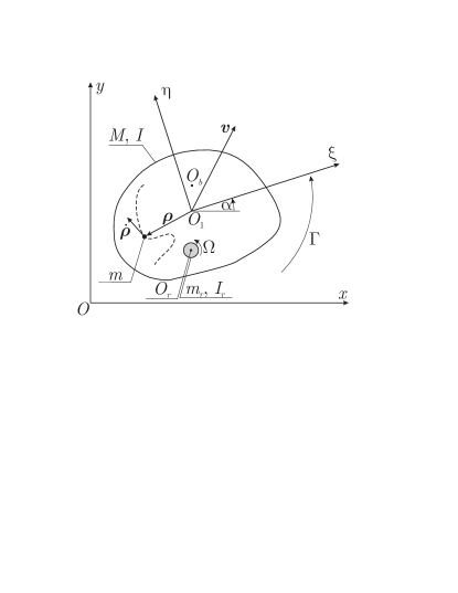
Figure 1: Body with an internal mass and an internal rotor

The body carries a particle of mass $m$ and a rotor with mass $m_{r}$ and central moment of inertia $I_{r}$. The motion of the particle is limited by the shell, but the particle follows an arbitrary smooth trajectory ${\boldsymbol{\rho}}=(\xi(t),\,\eta(t))$. The rotor has the shape of a circular cylinder, is homogeneous, rotates with angular velocity $\Omega(t)$; its axis of rotation is perpendicular to the plane of motion of the body and passes through the center of mass of the rotor. We assume that there is a nonzero and constant (by the Lagrange theorem) circulation $\Gamma$ of the fluid velocity around the body.

To describe the motion of the system, we introduce two Cartesian coordinate systems: a fixed one, $Oxy$, and a moving one, $O_{1}\xi\eta$, attached to the body (see Fig. 1). Point $O_{1}$ coincides with the position of the center of mass of the body–rotor system. The position of the body in absolute space is characterized by the radius vector ${\boldsymbol{r}}=(x,\,y)$ and the angle of rotation $\alpha$ of the moving coordinate system relative to the fixed coordinate system. Thus, the configuration space of the system is $\mathcal{H}=\mathbb{R}^{2}\times\mathbb{S}^{1}$, and the pair $({\boldsymbol{r}},\,\alpha)$ completely specifies the position and orientation of the body.

Let ${\boldsymbol{v}}=(v_{1},\,v_{2})$ denote the absolute velocity of point $O_{1}$ of the body referred to the axes of the moving coordinate system and $\omega$ the angular velocity of the body. Then the following kinematic relations hold:

$$\dot{{\boldsymbol{q}}}={\mathbb{Q}}{\boldsymbol{w}},\quad{\mathbb{Q}}=\begin{pmatrix}\cos\alpha&-\sin\alpha&0\\ \sin\alpha&\cos\alpha&0\\ 0&0&1\end{pmatrix}$$ (1)

where ${\boldsymbol{q}}=(x,\,y,\,\alpha)$ is the vector of generalized coordinates and ${\boldsymbol{w}}=(v_{1},\,v_{2},\,\omega)$ is the vector of quasi-velocities.

We specify the position of the body’s center of mass (point $O_{b}$) by the radius vector $(\xi_{b},\,\eta_{b})$ and the position of the rotor’s center of mass (point $O_{r}$) by the radius vector $(\xi_{r},\,\eta_{r})$. In the chosen coordinate system the coordinates of points $O_{b}$ and $O_{r}$ are related by

$$M\xi_{b}+m_{r}\xi_{r}=0,\quad M\eta_{b}+m_{r}\eta_{r}=0.$$

The expressions for the kinetic energy of the body $T_{b}$, the internal mass $T_{m}$, the internal rotor $T_{r}$ and the fluid $T_{f}$ have the form

$$T_{b}=\frac{1}{2}M\left((v_{1}-\eta_{b}\omega)^{2}+(v_{2}+\xi_{b}\omega)^{2}\right)+\frac{1}{2}I\omega^{2},$$

$$T_{m}=\frac{1}{2}m\left((v_{1}+\dot{\xi}-\eta\omega)^{2}+(v_{2}+\dot{\eta}+\xi\omega)^{2}\right),$$

$$T_{r}=\frac{1}{2}m_{r}\left((v_{1}-\eta_{r}\omega)^{2}+(v_{2}+\xi_{r}\omega)^{2}\right)+\frac{1}{2}I_{r}(\omega+\Omega)^{2},$$

$$T_{f}=\frac{1}{2}\lambda_{1}v_{1}^{2}+\frac{1}{2}\lambda_{2}v_{2}^{2}+\frac{1}{2}\lambda_{6}\omega^{2},$$

where $\lambda_{1}$ and $\lambda_{2}$ are the added masses ($\lambda_{1}\neq\lambda_{2}$), $\lambda_{6}$ is the added moment of inertia, and $\xi(t)$, $\eta(t)$, $\Omega(t)$ are known functions of time which play the role of controls in the system considered. With our choice of the origin of the moving coordinate system, the kinetic energy of the entire system is defined, up to the known functions of time, by the following expression:

$$T=\frac{1}{2}\left({\mathbb{A}}{\boldsymbol{w}},\,{\boldsymbol{w}}\right)+\left({\boldsymbol{u}},\,{\boldsymbol{w}}\right),$$ (2)

$${\mathbb{A}}=\begin{pmatrix}a_{1}&0&f\\ 0&a_{2}&g\\ f&g&b\end{pmatrix},\quad{\boldsymbol{u}}=\begin{pmatrix}m\dot{\xi}\\ m\dot{\eta}\\ m(\xi\dot{\eta}-\dot{\xi}\eta)+I_{r}\Omega\end{pmatrix},$$

$$a_{1}=M+m+m_{r}+\lambda_{1},\quad a_{2}=M+m+m_{r}+\lambda_{2},$$

$$b=M(\xi_{b}^{2}+\eta_{b}^{2})+I+m(\xi^{2}+\eta^{2})+m_{r}(\xi_{r}^{2}+\eta_{r}^{2})+I_{r}+\lambda_{6},\quad f=-m\eta,\quad g=m\xi.$$

The equations of motion of the system incorporating forces due to circulation around the body have the form

$$\begin{gathered}\frac{d}{dt}\left(\frac{\partial T}{\partial v_{1}}\right)=\omega\frac{\partial T}{\partial v_{2}}-\lambda v_{2}-\zeta\omega,\\ \frac{d}{dt}\left(\frac{\partial T}{\partial v_{2}}\right)=-\omega\frac{\partial T}{\partial v_{1}}+\lambda v_{1}+\chi\omega,\\ \frac{d}{dt}\left(\frac{\partial T}{\partial\omega}\right)=v_{2}\frac{\partial T}{\partial v_{1}}-v_{1}\frac{\partial T}{\partial v_{2}}+\zeta v_{1}-\chi v_{2},\end{gathered}$$ (6)

where $\lambda=\rho\Gamma$, $\zeta=\rho\Gamma\mu$, $\chi=\rho\Gamma\nu$, and $\mu$, $\nu$ are the coefficients associated with the hydrodynamical asymmetry of the body [10].

Equations (6) can be written in the form of Poincaré equations on the group $E(2)$

$$\begin{gathered}\frac{d}{dt}\left(\frac{\partial L}{\partial v_{1}}\right)=\omega\frac{\partial L}{\partial v_{2}}+\cos\alpha\frac{\partial L}{\partial x}+\sin\alpha\frac{\partial L}{\partial y},\\ \frac{d}{dt}\left(\frac{\partial L}{\partial v_{2}}\right)=-\omega\frac{\partial L}{\partial v_{1}}-\sin\alpha\frac{\partial L}{\partial x}+\cos\alpha\frac{\partial L}{\partial y},\\ \frac{d}{dt}\left(\frac{\partial L}{\partial\omega}\right)=v_{2}\frac{\partial L}{\partial v_{1}}-v_{1}\frac{\partial L}{\partial v_{2}}+\frac{\partial L}{\partial\alpha}\end{gathered}$$ (10)

with Lagrangian

$$L=\frac{1}{2}\left({\mathbb{A}}{\boldsymbol{w}},\,{\boldsymbol{w}}\right)+\left({\boldsymbol{c}},\,{\boldsymbol{w}}\right)+\left({\boldsymbol{u}},\,{\boldsymbol{w}}\right),$$ (11)

$${\boldsymbol{c}}=\begin{pmatrix}-\frac{\lambda}{2}(x\sin\alpha-y\cos\alpha)\\ -\frac{\lambda}{2}(x\cos\alpha+y\sin\alpha)\\ -\chi(x\sin\alpha-y\cos\alpha)-\zeta(x\cos\alpha+y\sin\alpha)\end{pmatrix}.$$

Equations (1), (10) form a closed system of six equations

$$\begin{gathered}\frac{d}{dt}(a_{1}v_{1}+f\omega+m\dot{\xi})=\omega(a_{2}v_{2}+g\omega+m\dot{\eta})-\lambda v_{2}-\zeta\omega,\\ \frac{d}{dt}(a_{2}v_{2}+g\omega+m\dot{\eta})=-\omega(a_{1}v_{1}+f\omega+m\dot{\xi})+\lambda v_{1}+\chi\omega,\\ \begin{split}\frac{d}{dt}(fv_{1}+gv_{2}+b\omega+m(\xi\dot{\eta}-\eta\dot{\xi})+I_{r}\Omega)={}&{}\\ =v_{2}(a_{1}v_{1}+f\omega+m\dot{\xi})-{}&{}v_{1}(a_{2}v_{2}+g\omega+m\dot{\eta})+\zeta v_{1}-\chi v_{2},\end{split}\\ \frac{dx}{dt}=v_{1}\cos\alpha-v_{2}\sin\alpha,\quad\frac{dy}{dt}=v_{1}\sin\alpha+v_{2}\cos\alpha,\quad\frac{d\alpha}{dt}=\omega\end{gathered}$$ (16)

in the variables $v_{1}$, $v_{2}$, $\omega$, $x$, $y$, $\alpha$ and completely describe the motion of the system considered.

For the case of a freely moving system, i.e., for $\dot{\xi}=\dot{\eta}=0$, $\Omega=0$, equations (16) admit the first integrals [10, 9]

$$\begin{gathered}p_{x}=\left(\frac{\partial L}{\partial v_{1}}-\chi\right)\cos\alpha-\left(\frac{\partial L}{\partial v_{2}}-\zeta\right)\sin\alpha+\frac{\lambda}{2}y,\\ p_{y}=\left(\frac{\partial L}{\partial v_{1}}-\chi\right)\sin\alpha+\left(\frac{\partial L}{\partial v_{2}}-\zeta\right)\cos\alpha-\frac{\lambda}{2}x,\\ K=xp_{y}-yp_{x}+\frac{\partial L}{\partial\omega}+\frac{\lambda}{2}(x^{2}+y^{2})-c_{3}.\end{gathered}$$ (20)

These integrals are generalized to the case of controlled motion and can be written in explicit form as follows:

$$\begin{gathered}p_{x}=(a_{1}v_{1}+f\omega+u_{1}-\chi)\cos\alpha-(a_{2}v_{2}+g\omega+u_{2}-\zeta)\sin\alpha+\lambda y,\\ p_{y}=(a_{1}v_{1}+f\omega+u_{1}-\chi)\sin\alpha+(a_{2}v_{2}+g\omega+u_{2}-\zeta)\cos\alpha-\lambda x,\\ K=fv_{1}+gv_{2}+b\omega+u_{3}+\frac{\lambda}{2}(x^{2}+y^{2})+xp_{y}-yp_{x}.\end{gathered}$$ (24)

The integrals $p_{x}$, $p_{y}$, $K$ have the meaning of the linear and angular momentum components of the body + control elements + fluid system and are a generalization of the integrals for a system with moving internal masses [21].

Note that (16) contains only the derivative $\dot{\Omega}$ (and not the angular velocity $\Omega$ itself), hence, the rotor rotating with constant angular velocity does not influence the dynamics of the system.

+

3 Controllability

To prove the controllability of motion on the fixed level set of first integrals, we shall use a modification of the Rashevskii-Chow theorem [1, 12, 27] for systems with drift [3]. This theorem requires, in addition to completeness of the linear span of the vector fields and their commutators, that there exists everywhere a dense set of Poisson stable points for the free motion (drift) in the phase space of the system.

The issue of Poisson stability of drift is considered in our previous paper [32]. In particular, it was shown that on the common level set of the integrals $p_{x}$ and $p_{y}$ the velocities $v_{1}$, $v_{2}$, and $\omega$ are related to the coordinates $x$ and $y$ by

$$(a_{1}v_{1}+f\omega-\chi)^{2}+(a_{2}v_{2}+g\omega-\zeta)^{2}=(p_{x}-\lambda y)^{2}+(p_{y}+\lambda x)^{2}$$ (25)

It is clear from (25) that the free motion is bounded by a circular region whose size and position depend on the level of the kinetic energy of the system $T$, the level sets of the integrals $p_{x}$ and $p_{y}$, the body geometry and circulation. In addition, the system of equations (1) and (10) is integrable; hence, by the Poincaré recurrence theorem [2], the free motion of the system is Poisson stable. Therefore, in what follows we shall investigate only the issue of completeness of the linear span of the vector fields and their commutators.

In [32] the controllability of motion by means of an internal mass capable of moving arbitrarily inside the body is proved. Therefore, an analogous system to which an internal rotor is added is controllable as well. In this section we prove controllability for two particular cases in which the following restrictions are imposed on possible motions of the internal mass:

1. The internal mass is fixed.

2. The internal mass moves along a given curve.

3.1 The case of a fixed internal mass

Let us examine the controllability of the system’s motion only by changing the rotation of the rotor. In this case, $\dot{\xi}=\dot{\eta}=0$, and the equations of motion (10) and the first integrals (24) are

$$\begin{gathered}\frac{d}{dt}\left(a_{1}v_{1}+f\omega\right)=\omega(a_{2}v_{2}+g\omega)-\lambda v_{2}-\zeta\omega,\\ \frac{d}{dt}\left(a_{2}v_{2}+g\omega\right)=-\omega(a_{1}v_{1}+f\omega)+\lambda v_{1}+\chi\omega,\\ \frac{d}{dt}\left(fv_{1}+gv_{2}+b\omega+I_{r}\Omega\right)=v_{2}(a_{1}v_{1}+f\omega)-v_{1}(a_{2}v_{2}+g\omega)+\zeta v_{1}-\chi v_{2}\end{gathered}$$ (29)

and

$$\begin{gathered}p_{x}=(a_{1}v_{1}+f\omega-\chi)\cos\alpha-(a_{2}v_{2}+g\omega-\zeta)\sin\alpha+\lambda y,\\ p_{y}=(a_{1}v_{1}+f\omega-\chi)\sin\alpha+(a_{2}v_{2}+g\omega-\zeta)\cos\alpha-\lambda x,\\ K=fv_{1}+gv_{2}+b\omega+I_{r}\Omega+\frac{\lambda}{2}(x^{2}+y^{2})+xp_{y}-yp_{x}.\end{gathered}$$ (33)

From the integrals $p_{x}$, $p_{y}$, and $K$ we express the velocities

$${\boldsymbol{w}}={\mathbb{A}}^{-1}\begin{pmatrix}\overline{x}\cos\alpha+\overline{y}\sin\alpha+\chi\\ -\overline{x}\sin\alpha+\overline{y}\cos\alpha+\zeta\\ F-\frac{1}{2\lambda}(\overline{x}^{2}+\overline{y}^{2})-I_{r}\Omega\end{pmatrix},$$ (34)

where $\overline{x}=p_{x}-\lambda y$, $\overline{y}=p_{y}+\lambda x$, $F=\dfrac{2K\lambda+p_{x}^{2}+p_{y}^{2}}{2\lambda}$. Substituting (34) into the kinematic relations (1), we obtain the equations of motion for the body on the fixed level set of the integrals $p_{x}$, $p_{y}$, $K$ in a standard form linear in the controls

$$\dot{{\boldsymbol{q}}}={\boldsymbol{V}}_{0}({\boldsymbol{q}})+{\boldsymbol{V}}_{1}\Omega,$$ (35)

$${\boldsymbol{V}}_{0}({\boldsymbol{q}})={\mathbb{S}}\left(\overline{x}\cos\alpha+\overline{y}\sin\alpha+\chi,\;-\overline{x}\sin\alpha+\overline{y}\cos\alpha+\zeta,\;F-\frac{1}{2\lambda}(\overline{x}^{2}+\overline{y}^{2})\right)^{T},$$

$${\boldsymbol{V}}_{1}={\mathbb{S}}(0,\;0,\;-I_{r})^{T},\quad{\mathbb{S}}={\mathbb{Q}}{\mathbb{A}}^{-1}.$$

Here the angular velocity of rotation of the rotor $\Omega$ is considered as control, the vector field ${\boldsymbol{V}}_{0}$ corresponds to the free motion (drift), and the vector field ${\boldsymbol{V}}_{1}$ is related to the control action. Consider the vector fields

$$\begin{gathered}{\boldsymbol{V}}_{0},\quad{\boldsymbol{V}}_{1},\quad{\boldsymbol{V}}_{2}=\left[{\boldsymbol{V}}_{0},\,{{\boldsymbol{V}}}_{1}\right],\quad{\boldsymbol{V}}_{3}=\left[{\boldsymbol{V}}_{2},\,{{\boldsymbol{V}}}_{1}\right],\end{gathered}$$ (37)

where $\left[\cdot,\,\cdot\right]$ is the Lie bracket. The rank of the linear span of the vector fields ${\boldsymbol{V}}_{0},\,{\boldsymbol{V}}_{1},\,{\boldsymbol{V}}_{3}$ is equal to three everywhere except on the surface given by

$$\begin{gathered}2(a_{2}^{2}-a_{1}^{2})\left((\overline{x}^{2}-\overline{y}^{2})\sin\alpha\cos\alpha-\overline{x}\overline{y}(\cos^{2}\alpha-\sin^{2}\alpha)\right)+\\ +a_{1}(2a_{1}-a_{2})\zeta(\overline{y}\sin\alpha+\overline{x}\cos\alpha)+a_{2}(2a_{2}-a_{1})\chi(\overline{x}\sin\alpha-\overline{y}\cos\alpha)=0.\end{gathered}$$ (40)

In a similar way, the rank of the linear span of the vector fields ${\boldsymbol{V}}_{1},\,{\boldsymbol{V}}_{2},\,{\boldsymbol{V}}_{3}$ is equal to three everywhere except on the surface given by

$$\begin{gathered}a_{1}^{2}\zeta^{2}+a_{2}^{2}\chi^{2}+2(a_{1}-a_{2})^{2}(\overline{x}^{2}+\overline{y}^{2})+\\ +3a_{1}(a_{2}-a_{1})\zeta(\overline{x}\sin\alpha-\overline{y}\cos\alpha)+3a_{2}(a_{2}-a_{1})\chi(\overline{y}\sin\alpha+\overline{x}\cos\alpha)=0.\end{gathered}$$ (43)

Remark 3.1.

The expressions (40) and (43) hold in the case where the moving coordinate system is chosen such that the matrix ${\mathbb{A}}$ takes the diagonal form ${\mathbb{A}}=\mathrm{diag}\,(a_{1},\,a_{2},\,b)$.

It is easy to show that the surfaces (40) and (43) intersect along the curves

$$\begin{gathered}\overline{x}=\left(\tau_{1}+\tau_{2}\right)\sin\alpha+\left(\tau_{1}-\tau_{2}\right)\cos\alpha,\\ \overline{y}=-\left(\tau_{1}+\tau_{2}\right)\cos\alpha+\left(\tau_{1}-\tau_{2}\right)\sin\alpha,\end{gathered}$$ (46)

where $\tau_{1}$ and $\,\tau_{2}$ are the solution of the system of equations

$$\begin{gathered}\left(8|a_{2}-a_{1}|\tau_{1}+3(a_{1}\zeta+a_{2}\chi)\right)^{2}+\left(8|a_{2}-a_{1}|\tau_{2}+3(a_{1}\zeta-a_{2}\chi)\right)^{2}-2\left(a_{1}^{2}\zeta^{2}+a_{2}^{2}\chi^{2}\right)=0,\\ \left(\tau_{1}+\frac{a_{2}(2a_{2}-a_{1})\chi+a_{1}(2a_{1}-a_{2})\zeta}{8(a_{2}^{2}-a_{1}^{2})}\right)^{2}-\left(\tau_{2}-\frac{a_{2}(2a_{2}-a_{1})\chi-a_{1}(2a_{1}-a_{2})\zeta}{8(a_{2}^{2}-a_{1}^{2})}\right)^{2}-\\ \\ -\frac{4a_{1}a_{2}(2a_{2}-a_{1})(2a_{1}-a_{2})\chi\zeta}{16(a_{2}^{2}-a_{1}^{2})}=0.\end{gathered}$$ (51)

Thus, in the configuration space $\mathcal{H}$ the dimension of the linear span of the vector fields (37) is equal to three everywhere except along the curves (46). Since the above curves are the surfaces of codimension two, the following theorem holds.

Theorem 3.1.

An arbitrary body moving in a fluid (in the presence of circulation around the body) with a given initial velocity can be moved by an appropriate rotation of the internal rotor from any initial position to any end position.

We note that the controllability proved in Theorem 3.1 is formal. Indeed, to construct control, the Rashevskii–Chow theorem uses the motion along the vector fields in both forward and backward time. When there is a drift, the motion along it is possible only in forward time. The motion in backward time is implemented by using the recurrence property of the trajectories. However, the calculation of the recurrence period in specific systems can be a fairly complicated problem (which can even defy a solution, for example, in the case of chaotic systems with measure), and the period itself can be very large or even tend to infinity. Thus, an appropriate construction of such controls is impossible.

For the chosen control method the presence of circulation is a necessary condition for controllability. Indeed, it is easy to show that for $\Gamma=0$ the system (35) becomes uncontrollable in the sense of Rashevskii–Chow. On the other hand, it follows from (35) that the drift caused by circulation cannot be completely compensated for by rotating the rotor. Therefore, in what follows we consider a combined model of controlling by both the rotor and the moving internal mass.

3.2 The case of motion of the internal mass along a given curve

We shall assume that the internal mass can move only along some curve ${\boldsymbol{\rho}}=(\xi(s),\eta(s))$, where $s$ is a parameter of the curve. From the integrals (24) we express the velocities

$${\boldsymbol{w}}={\mathbb{A}}^{-1}\begin{pmatrix}\overline{x}\cos\alpha+\overline{y}\sin\alpha+\chi-m\frac{d\xi}{ds}\dot{s}\\ -\overline{x}\sin\alpha+\overline{y}\cos\alpha+\zeta-m\frac{d\eta}{ds}\dot{s}\\ F-\frac{\overline{x}^{2}+\overline{y}^{2}}{2\lambda}-m(\xi\frac{d\eta}{ds}-\eta\frac{d\xi}{ds})\dot{s}-I_{r}\Omega\end{pmatrix}.$$ (52)

Substituting (52) into the kinematic relations (1), we obtain the equations of motion for the body on the fixed level set of the integrals (24). These equations depend on both the position $s$ of the mass on the curve and its velocity $\dot{s}$. Applying the standard method for phase space extension (Goh transformation [4]), we obtain the equations of motion in the form linear in the controls

$$\dot{{\boldsymbol{z}}}={\boldsymbol{V}}_{0}({\boldsymbol{z}})+{\boldsymbol{V}}_{1}(s)\dot{s}+{\boldsymbol{V}}_{2}\Omega,$$ (53)

$${\boldsymbol{V}}_{0}({\boldsymbol{z}})={\mathbb{R}}\left(\overline{x}\cos\alpha+\overline{y}\sin\alpha+\chi,\,-\overline{x}\sin\alpha+\overline{y}\cos\alpha+\zeta,\,F-\frac{\overline{x}^{2}+\overline{y}^{2}}{2\lambda},\,0\right)^{T},$$

$${\boldsymbol{V}}_{1}(s)={\mathbb{R}}\left(-m\frac{d\xi}{ds},\,-m\frac{d\eta}{ds},\,m\left(\eta\frac{d\xi}{ds}-\xi\frac{d\eta}{ds}\right),\,1\right)^{T},\quad{\boldsymbol{V}}_{2}={\mathbb{R}}\left(0,\,0,\,-I_{r},\,0\right)^{T},$$

$${\mathbb{R}}=\begin{pmatrix}{\mathbb{Q}}{\mathbb{A}}^{-1}&0\\ 0&1\end{pmatrix}.$$

Here ${\boldsymbol{z}}=(x,\,y,\,\alpha,\,s)^{T}$ is the vector in the expanded phase space $\mathcal{G}$. Note that not the coordinates of the internal mass, but its velocity of motion along the curve $\dot{s}$ and the angular velocity of the rotor $\Omega$ are taken as controls. The vector field ${\boldsymbol{V}}_{0}$ corresponds to the drift, and the vector fields ${\boldsymbol{V}}_{1}$, ${\boldsymbol{V}}_{2}$ are associated with the control actions. We consider the vector fields

$$\begin{gathered}{\boldsymbol{V}}_{1},\quad{\boldsymbol{V}}_{2},\quad{\boldsymbol{V}}_{3}=[{\boldsymbol{V}}_{1},\,{\boldsymbol{V}}_{2}],\quad{\boldsymbol{V}}_{4}=[{\boldsymbol{V}}_{1},\,{\boldsymbol{V}}_{3}],\quad{\boldsymbol{V}}_{5}=[{\boldsymbol{V}}_{2},\,{\boldsymbol{V}}_{3}],\quad{\boldsymbol{V}}_{6}=[{\boldsymbol{V}}_{1},\,{\boldsymbol{V}}_{4}]\end{gathered}$$ (55)

and show the completeness of their linear span. Here we deliberately do not consider the field ${\boldsymbol{V}}_{0}$, since in the case of completeness of the linear span of the vector fields (55) we also prove the controllability of motion for the case of zero circulation.

Consider separately two cases where the internal mass can move either along a straight line or along a circle. The choice of these curves is motivated by their simplicity.

1. We parameterize the reciprocating motion of the internal mass along the straight line as follows:

$$\xi=k_{1}\sin s,\quad\eta=k_{2}\sin s,$$ (56)

where $k_{1}$, $k_{2}$ are constants that do not vanish simultaneously. In this case, the vector fields ${\boldsymbol{V}}_{1}$, ${\boldsymbol{V}}_{2}$, ${\boldsymbol{V}}_{3}$, ${\boldsymbol{V}}_{5}$ are dependent for

$$s=\pi/2\leavevmode\nobreak\ \mbox{and}\leavevmode\nobreak\ s=3\pi/2.$$ (57)

On the surfaces given by (57), the condition of linear dependence of the vector fields ${\boldsymbol{V}}_{1}$, ${\boldsymbol{V}}_{2}$, ${\boldsymbol{V}}_{4}$, ${\boldsymbol{V}}_{6}$ is

$$A\sin\alpha+B\cos\alpha=0,$$ (58)

where $A$ and $B$ are the coefficients of rather complicated form which depend only on the system parameters. Thus, the rank of the linear span of the vector fields (55) is four everywhere in the phase space $\mathcal{G}$ except on the surface of codimension two, defined by (57) and (58). Hence, the following theorem holds.

Theorem 3.2.

An arbitrary body moving in a fluid (regardless of the presence of circulation around the body) with a given initial velocity can be moved by means of reciprocating motions of the internal mass and by rotating the internal rotor from any initial position to any final position with any initial and final positions of the internal mass.

2. We parameterize the motion of the internal mass in a circle as follows:

$$\xi=r_{o}\cos s,\quad\eta=r_{o}\sin s,\quad r_{o}>0.$$ (59)

It is easy to show that in this case the vector fields ${\boldsymbol{V}}_{1}$, ${\boldsymbol{V}}_{2}$, ${\boldsymbol{V}}_{3}$, ${\boldsymbol{V}}_{5}$ are independent in the entire space $\mathcal{G}$. Hence, the following theorem holds.

Theorem 3.3.

An arbitrary body moving in a fluid (regardless of the presence of circulation around the body) with a given initial velocity can be moved by means of the motion of the internal mass in a circle and by rotating the internal rotor from any initial position to any final position with any initial and final positions of the internal mass.

4 Stabilization of the body at a given point

4.1 Equations for controls

Consider the stabilization of the body at a given point. Without loss of generality we assume that the system has started its motion from the origin of coordinates $x(0)=y(0)=0$ with the initial orientation $\alpha(0)=0$, the rotor and the movable mass being at rest. In this case the motion of the system occurs on the level set of the integrals

$$p_{x}=-\chi,\quad p_{y}=-\zeta,\quad K=0,\quad F=\frac{\chi^{2}+\zeta^{2}}{2\lambda}.$$ (60)

Suppose that over some interval the body moved under the control action and came at time $t=T$ to the point $(x,\,y)$ with orientation $\alpha$. Let us formulate the problem of the body stabilization at this point as follows:

Can one choose limited control actions $\xi(t)$, $\eta(t)$ and $\Omega(t)$ at $t\geqslant T$ such that the body will stay arbitrarily long at point $(x,\,y)$ (possibly rotating about a fixed point).

If a stabilization occurs without rotation ($\dot{\alpha}=0$), we shall call it a complete stabilization, while a stabilization occurs with rotation about a fixed point ($\dot{\alpha}\neq 0$) will be called a partial stabilization. We impose the condition of limitation of control actions taking into account the possibility of their technical realization. In particular, the position of the moving mass is restricted by the boundary of the body, and the velocity of its motion and the rotor’s rotation are restricted by the capabilities of the motors.

Since the controlled motion is described by the system of differential equations (53) in the expanded space, this problem may be viewed as a particular case of the problem of controlling a part of variables. Therefore, the solution of this problem reduces not to the solution of some system of algebraic equations, but to analysis of differential equations governing the evolution of control actions $\xi(t)$, $\eta(t)$, $\Omega(t)$ and the remaining ”free” variable $\alpha(t)$.

To define these equations, we substitute the equalities $\dot{x}=\dot{y}=0$ into the first three equations of the system (53). As a result, we obtain the system of differential equations in $\xi(t)$, $\eta(t)$, $\alpha(t)$ which contains an unknown function $\Omega(t)$

$${\mathbb{D}}\frac{d}{dt}\begin{pmatrix}\xi\\ \eta\\ \alpha\end{pmatrix}=\begin{pmatrix}\overline{x}\cos\alpha+\overline{y}\sin\alpha+\chi\\ -\overline{x}\sin\alpha+\overline{y}\cos\alpha+\zeta\\ \frac{\chi^{2}+\zeta^{2}}{2\lambda}-\frac{\overline{x}^{2}+\overline{y}^{2}}{2\lambda}\end{pmatrix}-\begin{pmatrix}0\\ 0\\ I_{r}\Omega\end{pmatrix},\quad{\mathbb{D}}=\begin{pmatrix}m&0&-m\eta\\ 0&m&m\xi\\ -m\eta&m\xi&b\end{pmatrix}.$$ (61)

We recall that $\overline{x}=p_{x}-\lambda y$, $\overline{y}=p_{y}+\lambda x$. Making the change of variables

$$\xi=\rho\cos\left(\varphi-\overline{\varphi}\right),\quad\eta=\rho\sin\left(\varphi-\overline{\varphi}\right),\quad\psi=\alpha+\varphi-\overline{\varphi}+\overline{\psi},$$

$$\overline{\psi}=\arctan\frac{\overline{x}}{\overline{y}},\quad\overline{\varphi}=\arctan\frac{\chi}{\zeta},$$

we can represent equations (61) as

$$\begin{gathered}m\rho\dot{\psi}=r\cos\psi+\sigma\cos\varphi,\\ m\dot{\rho}=r\sin\psi+\sigma\sin\varphi,\\ (m\rho^{2}+\overline{b})\dot{\psi}-\overline{b}\dot{\varphi}=C_{xy}-I_{r}\Omega,\end{gathered}$$ (65)

where we have used the notation

$$r=\sqrt{\overline{x}^{2}+\overline{y}^{2}},\quad\sigma=\sqrt{\chi^{2}+\zeta^{2}},\quad C_{xy}=\frac{\sigma^{2}-r^{2}}{2\lambda},$$

$$\overline{b}=b-m\rho^{2}=M(\xi_{b}^{2}+\eta_{b}^{2})+I+m_{r}(\xi_{r}^{2}+\eta_{r}^{2})+I_{r}+\lambda_{6}.$$

The system (65) contains three equations and four unknown functions $\rho$, $\psi$, $\varphi$, $\Omega$ and cannot be uniquely solved without using additional conditions. In what follows we consider several particular variations of the problem in which an answer to the question raised can be found.

4.2 Complete stabilization of the body

In the case of complete stabilization of the body we assume that the conditions $\dot{x}=\dot{y}=0$, $\dot{\alpha}=0$ are satisfied at $t>T$. In this case, the following proposition holds.

Proposition 4.1.

A complete stabilization of the body during an infinite interval of time is possible if and only if the center of the body (point $O_{1}$ in Fig. 1) is on the circle

$$x=\frac{\zeta}{\lambda}+\frac{\sqrt{\chi^{2}+\zeta^{2}}}{\lambda}\cos\theta,\quad y=-\frac{\chi}{\lambda}+\frac{\sqrt{\chi^{2}+\zeta^{2}}}{\lambda}\sin\theta,\quad\theta\in[0,\,2\pi)$$ (66)

and its orientation is given by

$$\alpha=\theta-\arctan\frac{\zeta}{\chi}-\frac{\pi}{2}.$$ (67)

The corresponding controls are equal to zero, i.e., the moving mass and the rotor are at rest.

Proof.

Necessity. Setting $\dot{\alpha}=0$ in (61), we obtain the equations for the control actions

$$\begin{gathered}m\dot{\xi}=\overline{x}\cos\alpha+\overline{y}\sin\alpha+\chi,\\ m\dot{\eta}=-\overline{x}\sin\alpha+\overline{y}\cos\alpha+\zeta,\\ I_{r}\Omega+m(\xi\dot{\eta}-\dot{\xi}\eta)=\frac{\chi^{2}+\zeta^{2}}{2\lambda}-\frac{\overline{x}^{2}+\overline{y}^{2}}{2\lambda}.\end{gathered}$$ (71)

Since the right-hand sides of the first two equations (71) are constant and in the general case are not equal to zero, $\xi$ and $\eta$ are linear functions of time. Hence, at a certain instant of time the internal mass will reach the boundary of the body and will have to stop. Thus, a stabilization during an infinite interval of time is possible only if the right-hand sides of the first two equations of (71) are equal to zero. Setting the right-hand sides of (71) to zero and expressing $x$ and $y$ from them, we obtain the equations for the circle (66) and the relation of the body’s orientation to a point on the circle (67).

By substituting the resulting coordinates of the points of stabilization into the third equation of (71), it is easy to check that all controls are equal to zero in this case.

Sufficiency. Substituting (66) and (67) into the integrals (24), we obtain a system of equations of the form

$${\mathbb{A}}{\boldsymbol{w}}+{\boldsymbol{u}}=0.$$ (72)

The nondegeneracy of the matrix ${\mathbb{A}}$ implies that when there are no controls (${\boldsymbol{u}}=0$) and the body is at the points (66) with orientation (67), the body is at rest (${\boldsymbol{w}}=0$). ∎

Remark 4.1.

For a complete stabilization of the body on the circle (66) the position of the internal mass is inessential.

Since a complete stabilization at an arbitrary point is possible only during a finite interval of time, we consider the partial stabilization, i.e., $\dot{x}=\dot{y}=0$, $\dot{\alpha}\neq 0$, by using (65). In particular, we consider separately two cases in which additional restrictions (see Section 3) are imposed on the motion of the internal mass:

1. partial stabilization by rotating the rotor and by moving the internal mass in a circle ($\rho=\mathrm{const}\,$).

2. partial stabilization by rotating the rotor and by moving the internal mass along a straight line fixed in the body ($\varphi\leavevmode\nobreak\ =\leavevmode\nobreak\ \mathrm{const}\,$).

4.3 Partial stabilization at $\rho=\mathrm{const}\,$

Consider the partial stabilization in the case where the internal mass can move only in the circle of a given radius. For $\rho=\overline{\rho}=\mathrm{const}\,$, equations (65) take the form

$$\begin{gathered}m\overline{\rho}\dot{\psi}=r\cos\psi+\sigma\cos\varphi,\\ r\sin\psi+\sigma\sin\varphi=0,\\ (m\overline{\rho}^{2}+\overline{b})\dot{\psi}-\overline{b}\dot{\varphi}=C_{xy}-I_{r}\Omega.\end{gathered}$$ (76)

The first two equations of (76) form a closed system whose solution can yield the functions $\varphi(t)$ and $\psi(t)$. Then, using the known functions $\varphi(t)$ and $\psi(t)$ from the third equation of (76), we can express the dependence $\Omega(t)$

$$\Omega=\frac{1}{I_{r}}\left(C_{xy}-\frac{1}{m\overline{\rho}}(r\cos\psi+\sigma\cos\varphi)\left(m\overline{\rho}^{2}+\overline{b}+\overline{b}\frac{r\cos\psi}{\sigma\cos\varphi}\right)\right).$$ (77)

Remark 4.2.

At the initial instant of time the functions $\varphi$ and $\psi$ must satisfy the second equation of (76). This condition can be fulfilled by choosing the initial position of the internal mass. The possibility of choosing this initial position is ensured by Theorem 3.3, from which it follows that we can bring the body to the end point with an arbitrary position of the moving mass.

The solution of the system of equations (76) depends on the relationship between the parameters $r$ and $\sigma$. By a direct substitution it is easy to show that the condition $r=\sigma$ corresponds to the points of the circle (66). This circle divides the plane $(x,\,y)$ into two regions (see Fig. 2), in which the solution of the system (76) is different. Moreover, in what follows we shall prove that the following proposition holds.

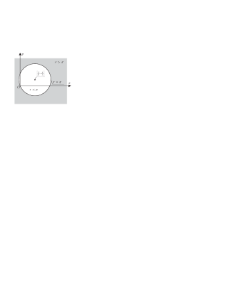
Figure 2: Regions of various solutions

Proposition 4.2.

A partial stabilization during an infinite interval of time by rotating the rotor and by moving the internal mass in a circle is possible only inside and on the circle $r=\sigma$ (see Fig. 2)

The proof of Proposition 4.2 is given in Appendix .

4.4 Partial stabilization for $\varphi=\mathrm{const}\,$

Consider a partial stabilization in the case where the internal mass can move only along a straight line fixed in the body. The controllability in this case was proved in Theorem 3.2. In the first two equations of (65) we set $\varphi=\varphi_{0}=\mathrm{const}\,$. Then they take the form

$$\begin{gathered}m\rho\dot{\psi}=r\cos\psi+\sigma\cos\varphi_{0},\\ m\dot{\rho}=r\sin\psi+\sigma\sin\varphi_{0},\end{gathered}$$ (80)

Solving the system (80), we can obtain the functions $\varphi(t)$, $\rho(t)$. Then, using the known functions $\varphi(t)$ and $\rho(t)$ from the third equation of (65), we can express the velocity of rotation of the rotor

$$\Omega(t)=\frac{1}{I_{r}}\left(C_{xy}-\frac{m\rho^{2}+\overline{b}}{m\rho}(r\cos\psi+\sigma\cos\varphi_{0})\right).$$ (81)

Analysis of equations (80) and (81) shows that the following proposition holds.

Proposition 4.3.

A partial stabilization during an infinite interval of time by rotating the rotor and by means of reciprocating motions of the internal mass in a circle is possible only inside and on the circle $r=\sigma$ (see Fig. 2)

The proof of Proposition 4.3 is given in Appendix B.

5 Conclusion

The investigation has shown that the motion of a hydrodynamically asymmetric body in an ideal fluid in the presence of circulation around the body is completely controllable (in the sense of the Rashevskii-Chow theorem) by changing the position of the center of mass (the motion of the internal mass is a motion in a circle or a reciprocating motion) and the angular momentum of the system. Moreover, an arbitrary motion of the system can be performed only by means of an appropriate rotation of the internal rotor.

We have also considered the possibility of compensation of drift by means of control. In particular, it was shown that by means of circular or reciprocating motion of the internal mass and by rotating the rotor the drift can be compensated for during an infinite interval of time if the body is inside some circular region. The center and the radius of this region are defined by the body geometry and by the amount of circulation of the velocity around the body. Outside this region, the drift can be compensated for using the above-mentioned patterns of motion of the internal mass only during a finite interval of time.

We list a number of open problems that must be solved to design real devices:

1. Construction of sufficiently simple and feasible patterns of motion of the internal mass to ensure a complete stabilization of the body at an arbitrary point of space during an infinite interval of time.

2. Construction of explicit control to ensure the motion from one point of space to another.

3. Motion control by variable circulation. For the case where circulation is a piecewise constant function of time, this problem has been solved in [26]. In this case, preservation of first integrals of motion was used on the intervals of constant circulation. Of great interest is a more general problem, namely, that of constructing controls by changing circulation according to a smooth law, when the system admits no first integrals of motion.

The authors thank A.V.Borisov and I.S.Mamaev for fruitful discussions.

The work of E.V. Vetchanin was supported by the RFBR grant 15-08-09093-a. The work of A.A. Kilin was supported by the RFBR grant 14-01-00395-a.

6 Appendix A. Proof of Proposition 4.2

Proof.

We break up the proof into three stages.

1. For $r<\sigma$ the second equation of (76) has two nonintersecting solutions

$$\varphi=\begin{cases}-\arcsin\left(\dfrac{r}{\sigma}\sin\psi\right)\in\left[-\arcsin\dfrac{r}{\sigma},\,\arcsin\dfrac{r}{\sigma}\right]\subset\left[-\dfrac{\pi}{2},\,\dfrac{\pi}{2}\right]\\ \pi+\arcsin\left(\dfrac{r}{\sigma}\sin\psi\right)\in\left[\pi-\arcsin\dfrac{r}{\sigma},\,\pi+\arcsin\dfrac{r}{\sigma}\right]\subset\left[\dfrac{\pi}{2},\,\dfrac{3\pi}{2}\right]\end{cases}$$ (82)

where $\psi\in[-\pi,\,\pi]$. The realization of a specific branch of the solution (82) depends on the initial value of $\varphi$, which is determined by the position of the internal mass at the instant of arrival at the point $(x,\,y)$. Moreover, according to Theorem 3.3 of complete controllability proved above, one can ensure, using appropriate controls, the realization of the required branch of the solution (82) at the initial instant of time.

Consider the branch $\varphi\in\left[-\arcsin\dfrac{r}{\sigma},\,\arcsin\dfrac{r}{\sigma}\right]$. Then $\cos\varphi>0$, and the first equation of (76), using the second equation, takes the form

$$m\overline{\rho}\dot{\psi}=r\cos\psi+\sigma\sqrt{1-\dfrac{r^{2}}{\sigma^{2}}\sin^{2}\psi}.$$ (83)

Equation (83) has the following solution:

$$E\left(\psi,\,\frac{r}{\sigma}\right)-E\left(\psi_{0},\,\frac{r}{\sigma}\right)-\frac{r}{\sigma}(\sin\psi-\sin\psi_{0})=\frac{\sigma^{2}-r^{2}}{m\overline{\rho}\sigma}t,$$ (84)

where $E\left(\psi,\,\dfrac{r}{\sigma}\right)$ is the normal elliptic Legendre integral of the second kind. The right-hand side of (83) is positive for any value of the angle $\psi$, hence, the function $\psi(t)$ increases monotonically. For the parameter values $\chi=0.1$, $\zeta=0.2$, $\lambda=1.0$, $I_{r}=1.0$, $m=1.0$, $\overline{\rho}=1.0$, $\overline{b}=2.0$, $x=0.1$, $y=0.0$, $\varphi\in\left[-\arcsin\dfrac{r}{\sigma},\,\arcsin\dfrac{r}{\sigma}\right]$ the form of the functions $\psi$, $\varphi$, $\Omega$ is shown in Fig. 3.

Figure 3: Form of the functions $\psi$, $\varphi$, $\Omega$ for the parameter values $\chi=0.1$, $\zeta=0.2$, $\lambda=1.0$, $I_{r}=1.0$, $m=1.0$, $\overline{\rho}=1.0$, $\overline{b}=2.0$, $x=0.1$, $y=0.0$

The constructed control is periodic, restricted and ensures a partial stabilization during an arbitrarily long interval of time.

Consider the second branch of the solution (82) $\varphi\in\left[\pi-\arcsin\dfrac{r}{\sigma},\,\pi+\arcsin\dfrac{r}{\sigma}\right]$. The differential equation for the determination of $\psi$ has the form

$$m\overline{\rho}\dot{\psi}=r\cos\psi-\sigma\sqrt{1-\dfrac{r^{2}}{\sigma^{2}}\sin^{2}\psi}.$$ (85)

Its solution is expressed, just as for the first branch, in terms of the normal elliptic Legendre integral of the second kind:

$$E\left(\psi,\,\frac{r}{\sigma}\right)-E\left(\psi_{0},\,\frac{r}{\sigma}\right)+\frac{r}{\sigma}(\sin\psi-\sin\psi_{0})=-\frac{\sigma^{2}-r^{2}}{m\overline{\rho}\sigma}t.$$ (86)

A straightforward calculation shows that the controls corresponding to the second branch are restricted during an arbitrarily long interval of time also.

2. For $r=\sigma$ the second equation of (76) has two solutions

$$\varphi=\begin{cases}\psi+\pi.\\ -\psi\end{cases}$$ (87)

If the equality $\varphi=\psi+\pi$ holds at the instant of arrival at a given point of space, then the first equation of (76) takes the form

$$m\overline{\rho}\dot{\psi}=0$$ (88)

i.e., the point $\varphi=\psi+\pi$ is a fixed point of the system. By straightforward calculations one can readily verify that this case corresponds to the solution (66) with $\alpha=\overline{\varphi}-\overline{\psi}-\pi$.

If the equality $\varphi=-\psi$ holds at the instant of arrival at a given point of space, then the first equation of (76) takes the form

$$m\overline{\rho}\dot{\psi}=2r\cos\psi$$ (89)

Equation (89) has two steady-state solutions: a stable one, $\psi_{1}=\dfrac{\pi}{2}$, and an unstable one, $\psi_{2}=\dfrac{3\pi}{2}$. The general solution of this equation has the form

$$\frac{m\overline{\rho}}{4r}\ln\left|\frac{1+\sin\psi}{1-\sin\psi}\right|=t+C$$ (90)

where $C$ is the constant of integration. It is clear from the form of the general solution that the approach to the point $\psi_{1}$ occurs in infinite time.

The rotational velocity of the rotor can be calculated from the third equation of (76) and takes the form

$$\Omega=-\frac{m\overline{\rho}^{2}+2\overline{b}}{m\overline{\rho}I_{r}}2r\cos\psi,$$ (91)

whence it is clear that the value of $\Omega$ is finite. Thus, for $r=\sigma$ a stabilization is possible in infinite time.

3. For $r>\sigma$ it is more convenient to express $\psi$ from the second equation of (76) as follows:

$$\psi=\begin{cases}-\arcsin\left(\dfrac{\sigma}{r}\sin\varphi\right)\in\left[-\arcsin\dfrac{\sigma}{r},\,\arcsin\dfrac{\sigma}{r}\right]\subset\left[-\dfrac{\pi}{2},\,\dfrac{\pi}{2}\right]\\ \pi+\arcsin\left(\dfrac{\sigma}{r}\sin\varphi\right)\in\left[\pi-\arcsin\dfrac{\sigma}{r},\,\pi+\arcsin\dfrac{\sigma}{r}\right]\subset\left[\dfrac{\pi}{2},\,\dfrac{3\pi}{2}\right]\end{cases}$$ (92)

where $\varphi\in[-\pi,\,\pi]$. The realization of a specific branch of the solution (92) depends on the initial value of $\psi$, which is defined by the position of the internal mass and by the orientation of the body at the instant of arrival at the point $(x,\,y)$. Moreover, according to Theorem 3.3 of complete controllability proved above, using a suitable control one can ensure the realization of the required branch of the solution (92) at the initial instant of time. Consider the branch $\psi\in\left[-\arcsin\dfrac{\sigma}{r},\,\arcsin\dfrac{\sigma}{r}\right]$ of the solution (92). This branch corresponds to the inequality $\cos\psi>0$, and the differential equation for the determination of $\varphi$ is obtained from the second equation of (76) and has the form

$$\left(\frac{\sigma^{2}\cos^{2}\varphi}{\sqrt{r^{2}-\sigma^{2}\sin^{2}\varphi}}-\sigma\cos\varphi\right)\dot{\varphi}=\frac{r^{2}-\sigma^{2}}{m\overline{\rho}}.$$ (93)

Let us examine the phase trajectories of (93). To do so, we express $\dot{\varphi}$ as follows:

$$\dot{\varphi}=\frac{r^{2}-\sigma^{2}}{2\overline{\rho}}\cdot\frac{\sqrt{r^{2}-\sigma^{2}\sin^{2}\varphi}}{\sigma\cos\varphi(\sigma\cos\varphi-\sqrt{r^{2}-\sigma^{2}\sin^{2}\varphi})}$$ (94)

In the case at hand, $\sigma\cos\varphi-\sqrt{r^{2}-\sigma^{2}\sin^{2}\varphi}<0$ always holds. Hence, $\dot{\varphi}(\varphi)$ undergoes a discontinuity of the second kind at the points $\varphi=\pm\dfrac{\pi}{2}$:

$$\lim_{\varphi\rightarrow\pm\frac{\pi}{2}\mp 0}\dot{\varphi}=-\infty,\quad\lim_{\varphi\rightarrow\mp\frac{\pi}{2}\pm 0}\dot{\varphi}=+\infty.$$ (95)

Note that these singularities do not depend on the value of $\dfrac{r}{\sigma}$. We also note that the function (94) does not vanish, and hence the system (94) has no fixed points.

The phase trajectories of (93) for $\dfrac{r}{\sigma}=1.1$ and various values of $\beta\leavevmode\nobreak\ =\leavevmode\nobreak\ \dfrac{r^{2}-\sigma^{2}}{m\overline{\rho}\sigma}$ are shown in Fig. 4

Figure 4: Phase trajectories of the system (94). The trajectories shown in the figure correspond to $\beta\leavevmode\nobreak\ =\leavevmode\nobreak\ 0.5$ and to various motion patterns.

Depending on the initial conditions, two motion patterns are possible for the same value of $\beta$. The corresponding functions $\varphi(t)$ and $\Omega(t)$ are shown in Figs. 5.

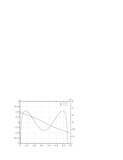
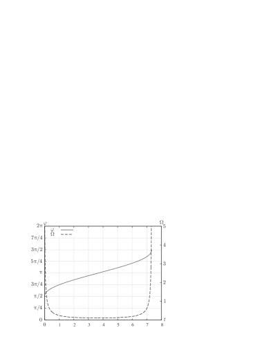
a)

b)

Figure 5: Functions $\varphi(t)$ and $\Omega(t)$ corresponding to different branches of the solution (82) for $\beta\leavevmode\nobreak\ =\leavevmode\nobreak\ 0.5$. The graphs correspond to the phase trajectories a) and b) in the previous figure.

It can be seen from Figs. 5 that the function $\varphi$ reaches the critical values $-\dfrac{\pi}{2}$ and $\dfrac{3\pi}{2}$ in finite time. Using (77), it is easy to check that $\Omega$ increases infinitely as $\varphi\rightarrow\pm\dfrac{\pi}{2}$. Hence, a partial stabilization is possible only in finite time.

Remark 6.1.

Equation (93) has the following solution:

$$\begin{split}\frac{\sigma^{2}-r^{2}}{r}\left(F\left(\varphi,\frac{\sigma}{r}\right)-F\left(\varphi_{0},\frac{\sigma}{r}\right)\right)+{}&{}r\left(E\left(\varphi,\frac{\sigma}{r}\right)-E\left(\varphi_{0},\frac{\sigma}{r}\right)\right)-\\ {}-{}&{}\sigma(\sin\varphi-\sin\varphi_{0})=\frac{r^{2}-\sigma^{2}}{m\overline{\rho}}t,\end{split}$$ (96)

where $F\left(\varphi,\,\dfrac{\sigma}{r}\right)$ is the normal elliptic Legendre integral of the first kind. The above solution (96) includes two motion patterns corresponding to different initial conditions $\varphi\in\left(-\dfrac{\pi}{2},\,\dfrac{\pi}{2}\right)$ and $\varphi\in\left(\dfrac{\pi}{2},\,\dfrac{3\pi}{2}\right)$.

A straightforward calculation shows that the solution corresponding to the branch $\psi\in\left[\pi-\arcsin\dfrac{\sigma}{r},\,\pi+\arcsin\dfrac{\sigma}{r}\right]$ behaves similarly. In this case, the equation for the determination of $\psi$ and its solution have the form

$$\left(\frac{\sigma^{2}\cos^{2}\varphi}{\sqrt{r^{2}-\sigma^{2}\sin^{2}\varphi}}+\sigma\cos\varphi\right)\dot{\varphi}=\frac{\sigma^{2}-r^{2}}{m\overline{\rho}},$$ (97)

$$\begin{split}\frac{\sigma^{2}-r^{2}}{r}\left(F\left(\varphi,\frac{\sigma}{r}\right)-F\left(\varphi_{0},\frac{\sigma}{r}\right)\right)+{}&{}r\left(E\left(\varphi,\frac{\sigma}{r}\right)-E\left(\varphi_{0},\frac{\sigma}{r}\right)\right)+\\ {}+{}&{}\sigma(\sin\varphi-\sin\varphi_{0})=\frac{\sigma^{2}-r^{2}}{m\overline{\rho}}t.\end{split}$$ (98)

∎

7 Appendix B. Proof of Proposition 4.3

Proof.

First of all, we examine the general properties of the system of equations (80)–(81). It is easy to verify that equations (80) possess the symmetry

$$\rho\rightarrow\rho,\quad\psi\rightarrow-\psi,\quad\varphi_{0}\rightarrow-\varphi_{0},\quad\Omega\rightarrow\Omega,\quad t\rightarrow-t$$ (99)

and the integral of motion

$$G=\rho e^{-\mathcal{F}(\psi)}=\mathrm{const}\,,\quad\mathcal{F}(\psi)=\int\frac{r\sin\psi+\sigma\sin\varphi_{0}}{r\cos\psi+\sigma\cos\varphi_{0}}d\psi.$$ (100)

The integral (100) and hence the behavior of the system depend on three parameters $r$, $\sigma$, and $\varphi_{0}$. The parameter $\varphi_{0}$ is related to the direction of motion of the internal mass, to circulation and the body geometry.

Below we consider separately several cases depending on the values of these parameters.

1. The condition $\sin\varphi_{0}=0$ corresponds to two values: $\varphi_{0}=0$ and $\varphi_{0}=\pi$, and the integral (100) takes the form

$$G=\rho(r\cos\psi\pm\sigma).$$ (101)

Here the sign $+$ corresponds to $\varphi_{0}=0$, and the sign $-$ corresponds to $\varphi_{0}=\pi$. In view of (101) the first equation of (80) takes the form

$$\dot{\psi}=\frac{1}{mG}(r\cos\psi\pm\sigma)^{2}.$$ (102)

Its solution depends on the relationship between the parameters $r$ and $\sigma$.

1.1. For $r<\sigma$ (the center of the body is inside the circle $r=\sigma$), according to (101), the function $\rho(t)$ has no singularities, is periodic and continuous for any value of $\psi$ and hence bounded on a given level set of the integral $G$. The right-hand side of (102) preserves the sign and never vanishes, hence, the function $\psi(t)$ is monotonous and equation (102) has no fixed points. An example of the functions $\rho(t)$, $\psi(t)$ and $\Omega(t)$ for $\varphi_{0}=0$ is shown in Fig. 6. Thus, for $\sin\varphi_{0}=0$ and $r<\sigma$ a partial stabilization is possible during an arbitrarily long interval of time.

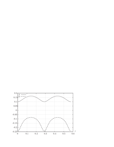
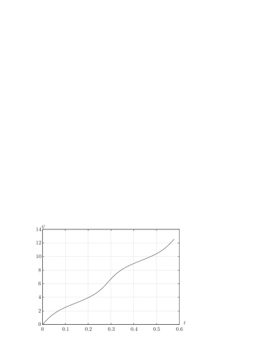
Figure 6: Functions $\rho(t)$, $\psi(t)$ and $\Omega(t)$

1.2. For $r=\sigma$ (the center of the body is on the circle $r=\sigma$) the system of equations (80) has a family of fixed points lying on the straight line $\psi=\psi_{*}=\pi+\varphi_{0}$. The phase trajectories of the system for $\varphi_{0}=\pi$ and various values of the integral $G$ are shown in Fig. 7.

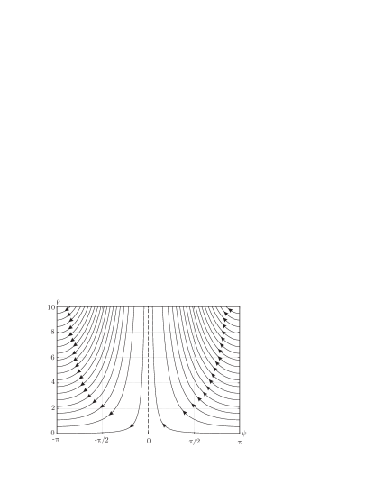
Figure 7: Phase trajectories of the system (80) for $\varphi_{0}=\pi$ and $\dfrac{r}{\sigma}=1$

It can be seen from Fig. 7 that the phase variable $\rho$ increases infinitely in a neighborhood of the straight line $\psi=\psi_{*}$.

Let us examine the attainability of a fixed point. To do so, we linearize equation (102) in its neighborhood

$$\dot{\psi}=\frac{r^{2}\sin^{2}\psi_{*}}{mG}(\psi-\psi_{*})^{2}.$$ (103)

Let us integrate equation (103) on the interval $[\psi_{*}-\varepsilon,\,\psi_{*})$

$$t\frac{r^{2}\sin^{2}\psi_{*}}{mG}=\frac{1}{\varepsilon}-\lim_{\psi\rightarrow\psi_{*}}\frac{1}{\psi-\psi_{*}}=\infty.$$ (104)

Consequently, the phase trajectories approach the straight line $\psi=\psi_{*}$ in infinite time. Thus, for $\sin\varphi_{0}=0$ and $r=\sigma$ a partial stabilization can be performed only in finite time.

1.3. For $r>\sigma$ (the center of the body is outside the circle $r=\sigma$), equation (102) admits particular steady-state solutions

$$\psi^{*}_{\pm}=\begin{cases}\pm\left(\pi-\arccos\frac{\sigma}{r}\right),&\varphi_{0}=0,\\ \pm\arccos\frac{\sigma}{r},&\varphi_{0}=\pi.\end{cases}$$ (105)

The phase trajectories of the system on the plane $(\rho,\,\psi)$ for various values of the integral $G$ and the parameter values $r=1$, $\sigma=0.5$ are shown in Fig.8.

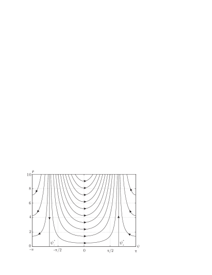
Figure 8: Phase trajectories of the system (80) for $\sin\varphi_{0}=0$ and $\dfrac{r}{\sigma}>1$

It can be seen from Fig.8 that the phase trajectories approach the vertical asymptotes $\psi=\psi^{*}_{\pm}$, hence, as time goes on, $\rho\rightarrow+\infty$. Performing the same analysis as in the previous case, we can show that the value $\psi=\psi_{+}$ is reached in infinite time. Thus, for $\sin\varphi_{0}=0$ and $r>\sigma$ a partial stabilization can be performed only in finite time.

2. Consider a more general case for which the line of motion of the internal mass is such that $\sin\varphi_{0}\neq 0$. In this case, the integral (100) can be written as

$$G=\rho(r\cos\psi+\overline{\sigma})\exp\left(-\sigma\sin\varphi_{0}\int\frac{d\psi}{r\cos\psi+\overline{\sigma}}\right)=\mathrm{const}\,,\quad\overline{\sigma}=\sigma\cos\varphi_{0}.$$ (106)

The exact form of the integral (106) depends on the relationship between $r$ and $\sigma|\cos\varphi_{0}|$. The equality $r=\sigma|\cos\varphi_{0}|$ defines the circle with the center at the point $\left(\dfrac{\zeta}{\lambda},\,-\dfrac{\chi}{\lambda}\right)$ and radius $\dfrac{\sqrt{\chi^{2}+\zeta^{2}}}{\lambda}|\cos\varphi_{0}|$.

2.1. For $r<\sigma|\cos\varphi_{0}|$ (the center of the body is inside the circle $r=\sigma|\cos\varphi_{0}|$) the integral (106) is not unique and can be represented as

$$\overline{G}=\frac{G}{r}=\rho(\cos\psi+\varkappa)\times\\ \times\exp\left(-\frac{2\varkappa\tan\varphi_{0}}{\sqrt{\varkappa^{2}-1}}\left(\arctan\left(\frac{\sqrt{\varkappa^{2}-1}}{\varkappa+1}\tan\frac{\psi}{2}\right)+\left[\frac{\psi+\pi}{2\pi}\right]\pi\right)\right)=\mathrm{const}\,,$$ (107)

where $\varkappa=\dfrac{\overline{\sigma}}{r}$, $|\varkappa|>1$, $\psi\in[-\pi,\,\pi)$.

The trajectories of the system (80) fill everywhere densely the plane $(\rho,\,\psi)$. Depending on the relationship between the parameters $r$, $\sigma$, and $\varphi_{0}$, two types of phase portraits are possible (see Fig. 9).

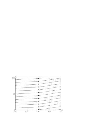
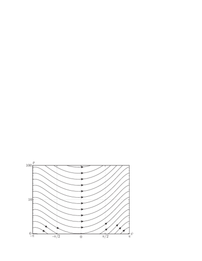
a)                                                                       b)

Figure 9: Phase portraits of the system for $\sigma=1.5$, $\varphi_{0}=0.1$. a) $r=0.1$, b) $r=1$

Indeed, the right-hand side of the second equation of (80) is nonnegative (nonpositive) for $\dfrac{\sigma|\sin\varphi_{0}|}{r}\geqslant 1$. This means nondecrease (nonincrease) of the function $\rho$ (see Fig. 9a). Otherwise the sign $\dot{\rho}$ changes twice in one period of the variable $\psi$, and the system trajectories have extrema (see Fig. 9b).

According to the first equation of (80), the function $\psi(t)$ is monotonous, since the right-hand side of the equation is sign-definite by virtue of the condition $r<\sigma|\cos\psi_{0}|$. Using the integral (107), we estimate the change of $\rho$ for one period of the variable $\psi\in[-\pi,\,\pi)$

$$\Delta\rho=\rho_{0}\left(\exp\left(\frac{2\pi\varkappa\tan\varphi_{0}}{\sqrt{\varkappa^{2}-1}}\right)-1\right).$$ (108)

It can be seen from (108) that the increment $\Delta\rho$ of the phase variable $\rho$ is directly proportional to the value $\rho_{0}=\rho\big{|}_{\psi=-\pi}$. Moreover, $\mathrm{sign}\,\Delta\rho=\mathrm{sign}\,\tan\varphi_{0}$. It is easy to show that for $N$ periods the increment is

$$\Delta\rho_{N}=\rho_{0}\left(\exp\left(\frac{2N\pi\varkappa\tan\varphi_{0}}{\sqrt{\varkappa^{2}-1}}\right)-1\right).$$ (109)

That is, the increment depends exponentially on the number of periods $N$. Thus, despite the existence of two types of phase portraits, the phase variable $\rho$ increases on an average if $\tan\varphi_{0}>0$ and decreases on an average if $\tan\varphi_{0}<0$.

According to (81), as $\rho$ decreases infinitely, $\Omega\rightarrow\infty$. Thus, if the condition $r<\sigma|\cos\varphi_{0}|$ is satisfied, either $\rho$ or $\Omega$ increases indefinitely, depending on the value of $\varphi_{0}$. Thus, for $\sin\varphi_{0}\neq 0$ and $r=\sigma|\cos\varphi_{0}|$ a partial stabilization can be performed only in finite time.

2.2. For $r>\sigma|\cos\varphi_{0}|$ (the center of the body is outside the circle $r=\sigma|\cos\varphi_{0}|$) the integral (106) can be written as

$$\overline{G}=-\rho\frac{\mathrm{sign}\,(\tau_{+}(\psi)\tau_{-}(\psi))}{1+\tan^{2}\frac{\psi}{2}}|\tau_{-}(\psi)|^{\delta+1}|\tau_{+}(\psi)|^{1-\delta},$$ (110)

$$\delta=\frac{\varkappa\tan\varphi_{0}}{\sqrt{1-\varkappa^{2}}},\quad\tau_{\pm}(\psi)=\sqrt{1-\varkappa}\tan\frac{\psi}{2}\pm\sqrt{1+\varkappa}.$$

Consider the values $\psi_{\pm}=\mp 2\arctan\sqrt{\frac{1+\varkappa}{1-\varkappa}}$, which are zeros of the functions $\tau_{\pm}(\psi)$. It is seen from (110) that the behavior of the system (80) in a neighborhood of the lines $\psi=\psi_{\pm}$ can change depending on the parameter $\delta$. For the values $\delta<0$ three possible types of phase portraits are shown in Fig. 10.

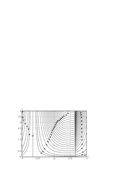
a)                                         b)                                         c)

Figure 10: a) $\delta=-0.5$, b) $\delta=-1$, c) $\delta=-1.1$

Remark 7.1.

By virtue of the symmetry (99), the phase portrait for some $\delta=-\delta_{0}<0$ can be obtained by a mirror reflection of the phase portrait for $\delta=\delta_{0}$ relative to $\psi=0$ and by changing the direction of motion along the trajectories.

2.2.1. If $|\delta|<1$, the phase variable $\rho$ infinitely increases near $\psi_{\pm}$. The asymptotes $\psi=\psi_{\pm}$ are always separated from each other regardless of the relationship between the parameters $r$, $\sigma$, and $\varphi_{0}$. Hence, the qualitative behavior of the system trajectories on the plane $(\rho,\,\psi)$ (see Fig. 10a) is also independent of the relationships between these parameters and is the same as the behavior considered in the case $\sin\varphi_{0}=0$, $r>\sigma$ (see Fig. 8). Thus, for $\sin\varphi_{0}\neq 0$ and $r<\sigma|\cos\varphi_{0}|$ a partial stabilization can be performed only in finite time.

2.2.2. The condition $|\delta|=1$ is equivalent to the equality $r=\sigma$. In this case, the right-hand sides of equations (80) vanish simultaneously for $\psi=\pi+\varphi_{0}$. When $\delta=-1$, the asymptote $\psi=\psi_{-}$ disappears, and its place is taken by a family of fixed points; there are no qualitative changes in a neighborhood of the asymptote $\psi=\psi_{+}$ (see Fig. 10b). Similarly, when $\delta=1$, the lines $\psi=\psi_{+}$ correspond to a family of fixed points and $\psi=\psi_{-}$ is an asymptote. To perform a stability analysis of these fixed points, we represent the first equation of (80) as

$$m\rho\dot{\psi}=-\frac{r}{1+\tan^{2}\frac{\psi}{2}}\tau_{+}(\psi)\tau_{-}(\psi).$$ (111)

Let us analyze the stability of the family of fixed points $\psi=\psi_{-}$ for $\delta=-1$. For this purpose, we linearize equation (111) in a neighborhood of $\psi=\psi_{-}$

$$m\rho\dot{\Delta\psi}=-\frac{r}{1+\tan^{2}\frac{\psi_{-}}{2}}\tau_{+}(\psi_{-})\frac{\sqrt{1-\varkappa}}{2\cos^{2}\frac{\psi_{-}}{2}}\Delta\psi,\quad\psi=\psi_{-}+\Delta\psi.$$ (112)

Since the coefficient of $\Delta\psi$ is negative, the fixed points of the family $\psi=\psi_{-}$ are stable. In a similar way, it can be shown that the fixed points of the family $\psi=\psi_{+}$ are unstable for $\delta=1$. Since $\mathrm{sign}\,\delta=\mathrm{sign}\,\tan\varphi_{0}$, the system has the above family of stable fixed points for $\tan\varphi_{0}<0$, and the family of unstable fixed points for $\tan\varphi_{0}>0$. Thus, a partial stabilization is possible in infinite time when $\sin\varphi_{0}\neq 0$, $r>\sigma|\cos\varphi_{0}|$ and $\delta=-1$.

2.2.3. Consider the behavior of the system for $|\delta|>1$. The phase portrait corresponding to $\delta<-1$ is shown in Fig. 10c. The behavior in a neighborhood of the straight line $\psi=\psi_{+}$ does not change qualitatively. In contrast to the cases considered above, the line $\psi=\psi_{-}$ becomes a discontinuity of the integral $\overline{G}$. Note that due to equation (111) $\dot{\psi}>0$ for $\psi\in(\psi_{+},\,\psi_{-})$ and $\dot{\psi}<0$ for $\psi\in[-\pi/2,\,\psi_{+})\cup(\psi_{-},\,\pi/2]$. Thus, all trajectories of (80) tend to the point $\psi=\psi_{-}$, $\rho=0$ on a given level set of the integral $\overline{G}$.

The point $\psi=\psi_{-}$, $\rho=0$ is the singular point of (80). This singularity may be due to either the choice of polar coordinates or the existence of an essential singular point in the system. In order to define the type of singularity, it is necessary to examine the value of the limit $\lim\limits_{\rho\rightarrow 0}\dot{\rho}$ depending on $\psi$. This analysis for the system considered shows that the point $\psi=\psi_{-}$, $\rho=0$ is an essential singular point and all trajectories of the system converge to it.

Consider the attainability of the point $\psi=\psi_{-}$, $\rho=0$ in finite/infinite time. Let us eliminate $\rho$ from the first equation of (80) using the integral (110)

$$\dot{\psi}=\frac{1}{mG}\frac{1}{(1+\tan^{2}\frac{\psi}{2})^{2}}|\tau_{+}(\psi)|^{2-\delta}|\tau_{-}(\psi)|^{2+\delta}.$$ (113)

Equation (113) can be approximated by

$$\dot{\psi}=\Lambda(\psi-\psi_{-})^{2+\delta}$$ (114)

using the Taylor series expansion of the function $\tau_{-}(\psi)$ in a neighborhood of $\psi=\psi_{-}$. Without loss of generality we set $\psi-\psi_{-}>0$. Since $2+\delta<1$, the solution of (114) is the following power function:

$$\psi=\psi_{-}+(-(1+\delta)(\Lambda t+C))^{-1/(\delta+1)},$$ (115)

whence it is clear that the line $\psi=\psi_{-}$ is attained in finite time.

Let us consider the behavior of the angular velocity $\Omega$ as the line $\psi=\psi_{-}$ is approached. Expression (81) can be written as

$$\Omega=\frac{1}{I_{r}}\left(C_{xy}-(m\rho^{2}+\overline{b})\dot{\psi}\right).$$ (116)

It is seen from (114) and (116) that for $\delta\in(-2,\,-1)$ the derivative $\dot{\psi}$ tends to zero as $\psi=\psi_{-}$ is approached, hence, $\Omega\rightarrow\dfrac{C_{xy}}{I_{r}}$. If $\delta=-2$, then $\dot{\psi}=\Lambda$, hence, $\Omega\rightarrow\dfrac{C_{xy}-\overline{b}\Lambda}{I_{r}}$. If $\delta<-2$, then $\dot{\psi}\rightarrow\infty$, hence, $\Omega\rightarrow\infty$. Thus, a partial stabilization is possible in finite time for $\sin\varphi_{0}\neq 0$, $r>\sigma|\cos\varphi_{0}|$ and $|\delta|>1$. ∎

References

- [1] Agrachev A. A., Sachkov Y. Control theory from the geometric viewpoint. – Springer Science & Business Media, 2004.
- [2] Arnold V.I. Mathematical methods of classical mechanics. – Springer Science & Business Media, 1989.
- [3] Bonnard B. Contrôlabilité des systèmes nonlinéaires // C. R. Acad. Sci. Paris, Sér. 1. 1981. V. 292. P. 535–537.
- [4] Bonnard B., Chyba M. Singular trajectories and their role in control theory. Vol. 40. Springer Science & Business Media, 2003.
- [5] Bolotin S.V. The problem of optimal control of a Chaplygin ball by internal rotors // Rus. J. Nonlin. Dyn., 2012, vol. 8, no. 4, pp. 837–852 (Russian
- [6] Borisov A.V., Kilin A.A., Mamaev I.S. How to Control Chaplygin’s Sphere Using Rotors // Regul. Chaotic Dyn. 2012. V. 17 no. 3–4. pp. 258–272.
- [7] Borisov A.V., Kilin A.A., Mamaev I.S. How to Control the Chaplygin Ball Using Rotors. II // Regul. Chaotic Dyn., 2013, V. 18 no. 1–2, pp. 144–158.
- [8] Borisov A.V., Kozlov V.V., Mamaev I.S. Asymptotic stability and associated problems of failing rigid body // Regul. Chaotic Dyn. 2007. V. 12. no. 5. pp. 531–565.
- [9] Borisov A.V., Mamaev I.S. On the motion of a heavy rigid body in an ideal fluid with circulation, CHAOS, 2006, Vol. 16, no. 1, 013118 (7 pages)
- [10] Chaplygin S.A. On the influence of a plane-parallel flow of air on moving through it a cylindrical wing // Tr. Cent. Aerohydr. inst. 1926. Vyp. 19. pp. 300–382
- [11] Childress S., Spagnolie S. E., Tokieda T. A bug on a raft: recoil locomotion in a viscous fluid // J. Fluid Mech. 2011. V. 669. pp. 527–556.
- [12] Chow W. L. Über Systeme von linearen partiellen Differentialgleichungen erster Ordnung //Math. Ann. 1939. V. 117. no. 1. pp. 98-105.
- [13] Chyba M., Leonard N.E., Sontag E.D Optimality for underwater vehicles // IEEE, 1998, 2001, vol. 5, pp. 4204-4209.
- [14] Chyba M., Leonard N. E., Sontag E.D. Singular trajectories in multi-input time-optimal problems: Application to controlled mechanical systems //Journal of dynamical and control systems. – 2003. – V. 9. – no. 1. – P. 103-129.
- [15] Crouch P.E. Spacecraft Attitude Control and Stabilization: Applications of Geometric Control Theory to Rigid Body Models // IEEE Transactions on Automatic Control, 1984, vol. 29, no. 4, pp. 321-331
- [16] Ivanov A.P. On the Control of a Robot Ball Using Two Omniwheels, Regul. Chaotic Dyn., 2015, 20 (4), pp. 441-448.
- [17] Jurdjevic V. Geometric control theory. – Cambridge university press, 1997.
- [18] Kilin A.A., Vetchanin E.V. The contol of the motion through an ideal fluid of a rigid body by means of two moving masses, Nelin. Dinam., 2015, vol. 11, no. 4, pp. 633–645 (in Russian)
- [19] Kirchhoff G., Hensel K. Vorlesungen über mathematische Physik. Mechanik. Leipzig: BG Teubner, 1874. P.489
- [20] Kozlov V.V., Onishchenko D.A. The motion in a perfect fluid of a body containing a moving point mass // J. Appl. Math. Mech. 2003. V. 67. no. 4. P. 553–564
- [21] Kozlov V.V., Ramodanov S.M. On the motion of a variable body through an ideal fluid // PMM. 2001. V. 65. Vyp. 4. pp. 529–601
- [22] Lamb H. Hydrodynamics. New York: Dover, 1945. P.728
- [23] Leonard N.E., Marsden J.E. Stability and Drift of Underwater Vehicle Dynamics: Mechanical Systems with Rigid Motion Symmetry // Physica D: Nonlinear Phenomena. – 1997. – V. 105. – no. 1. – pp. 130-162
- [24] Leonard N.E. Stability of a bottom-heavy underwater vehicle // Automatica. – 1997. – V. 33. – no. 3. – pp. 331-346.
- [25] Murray R.M., Sastry S.S. Nonholonomic motion planning: steering using sinusoids // IEEE TRANSACTIONS ON AUTOMATIC CONTROL, 1993, vol. 38, no. 5, pp. 700-716
- [26] Ramodanov S. M., Tenenev V. A., Treschev D. V. Self-propulsion of a Body with Rigid Surface and Variable Coefficient of Lift in a Perfect Fluid // Regul. Chaotic Dyn. 2012 V.17 no. 6, P. 547–558.
- [27] Rashevskii P.K. About connecting two points of complete non-holonomic space by admissible curve (in Russian), Uch. Zapiski ped. inst. Libknexta (2): 83–94
- [28] Spindler K. Attitude maneuvers which avoid a forbidden direction //Journal of dynamical and control systems. – 2002. – V. 8. – no. 1. – V. 1-22.
- [29] Steklov V.A. On the motion of a rigid body through a fluid. Article 1 // Soob. Khark. mat. obsch. 1891. V. 2. no. 5–6. C.209–235
- [30] Svinin M., Morinaga A., Yamamoto M. On the Dynamic Model and Motion Planning for a Class of Spherical Rolling Robots // 2012 IEEE International Conference on Robotics and Automation, 2012, pp. 3226-3231
- [31] Vankerschaver J., Kanso E., Marsden J.E. The dynamics of a rigid body in potential flow with circulation // Regul. Chaotic Dyn. 2010 V. 15 no. 4–5. P. 606–629.
- [32] Vetchanin E.V., Kilin A.A. Free and controllable motion of a body through a fluid by means of an internal mass in the presence of circulation around the body // in press
- [33] Vetchanin E. V., Mamaev I. S., Tenenev V. A. The self-propulsion of a body with moving internal masses in a viscous fluid // Regul. Chaotic Dyn. 2013. V. 18. no. 1–2. P. 100–117.
- [34] Woolsey C.A., Leonard N.E. Stabilizing underwater vehicle motion using internal rotors // Automatica, 2002, vol. 38, no. 12, pp. 2053-2062