Coverage Analysis In Downlink Poisson Cellular Network With $\kappa$-$\mu$ Shadowed Fading

Abstract

The downlink coverage probability of a cellular network, when the base station locations are modelled by a Poisson point process (PPP), is known when the desired channel is Nakagami distributed with an integer shape parameter. However, for many interesting fading distributions such as Rician, Rician shadowing, $\kappa$-$\mu$, $\eta$-$\mu$, etc., the coverage probability is unknown. $\kappa$-$\mu$ shadowed fading is a generic fading distribution whose special cases are many of these popular distributions known so far. In this letter, we derive the coverage probability when the desired channel experiences $\kappa$-$\mu$ shadowed fading. Using numerical simulations, we verify our analytical expressions.

I Introduction

The downlink coverage probability of a single-tier cellular network with distance-dependent interference was analyzed in [1] using tools from stochastic geometry. This was followed by new results for multi-tier cellular networks in single antenna [2] and multi-antenna systems [3]. An important assumption in these works is that the fading distribution of the nearest (desired) base station (BS) is Rayleigh. Rayleigh fading is an important assumption as the channel power will follow exponential distribution. This allows the distribution of signal-to-interference ratio ($\mathtt{SIR}$) to be expressed in terms of the Laplace transform of interference which can easily be computed using standard tools from stochastic geometry. In a multi-antenna system that uses maximal-ratio combining, if the fading distribution of all the links are i.i.d. Rayleigh distributed, the channel power is Gamma distributed with integer shape parameter (equal to the number of antenna terminals). The coverage probability of such a system can be computed by using Laplace transform of interference and its derivative.

However, for popular channel fading distribution like Rician, the Laplace trick cannot be used as the complementary cumulative distribution function ($\mathtt{CCDF}$) of the channel power is not an exponential function. In [4], the coverage probability of a two-tier cellular network was obtained when the desired signal experiences Rician fading. This approach assumes that the $\mathtt{CCDF}$ of a non-central chi-squared distributed (square of Rician) random variable, can be approximated as a weighted sum of exponentials. The weights and abscissas are obtained by minimizing the mean squared error between the $\mathtt{CCDF}$ and this approximation. As the function minimized is not convex, the weights and abscissas obtained are locally optimal and are highly dependent on the initial points assumed. Also, there are no closed-form expressions available for these weights and abscissas and have to be computed numerically. In [5], the coverage probability of a single-tier network with an arbitrary fading distribution was derived using Gil-Pelaez inversion theorem. The coverage probability expression in [5] requires a numerical integration of the imaginary part of the moment generating function ($\mathtt{MGF}$) of the desired channel’s power. However, this approach requires numerical evaluation of multi-dimensional integrals for heterogeneous networks. In [6], it is shown that analytically tractable expressions for coverage probability of a heterogeneous cellular network can not be derived in presence of arbitrary fading if the tier association is based on maximum average received power. In [7], [8] average rate was derived for arbitrary fading channels and fading channels with dominant specular components respectively. But these approaches can not be used for evaluating the coverage probability.

In this letter, we assume all the channels to experience independent $\kappa$-$\mu$ shadowed fading and derive the exact coverage probability when the parameter $\mu$ of the desired channel is an integer and use “Rician approximation” to derive an approximate one when $\mu$ is not an integer. So using this method, the coverage probability can be obtained if the desired channel is Nakagami faded with non-integer shape parameter whereas the Laplace trick is useful only when the shape parameter is an integer. As the popular fading distributions such as Rician, Rayleigh, Nakagami, Rician shadowing, $\kappa$-$\mu$, $\eta$-$\mu$ are special cases of $\kappa$-$\mu$ shadowed fading, the coverage probability expression obtained is generic. Our analysis assumes that the single tier base stations are PPP distributed and the interfering signals fade independently and identically. The analysis can be easily extended to a multi tier heterogeneous network that uses maximum average received power based association following similar steps as in [2].

II System Model

The base stations are modelled by a homogeneous Poisson point process $\Phi$ $\subseteq$ $\mathbb{R}^{2}$ of intensity $\lambda$. All the base stations are assumed to transmit with unit power. The signal from a base station located at $x\in\mathbb{R}^{2},$ experiences a path loss $||x||^{-\alpha}$, where $\alpha>2.$ Without loss of generality, a typical user is assumed to be at the origin and is associated with the nearest base station located at a distance $r$. Nearest base station association in a single tier network is same as the maximum average received power based association [2]. This is preferred to the highest $\mathtt{SIR}$ based association so that frequent handovers that occurs due to short term fading and shadowing can be avoided [2]. From [1], the nearest neighbour distance is Rayleigh distributed, i.e., $f(r)=2\pi\lambda r\exp(-\pi\lambda r^{2})$. The system is assumed to be interference limited and hence noise is neglected.

III $\kappa$-$\mu$ shadowed fading

$\kappa$-$\mu$ shadowed fading is represented by three parameters viz. $\kappa$, $\mu$ and $m$. Let $\gamma$ denote the signal power. The probability density function of the signal power when the channel experiences $\kappa$-$\mu$ shadowed fading [9] is denoted by $f(\gamma)$ and is given as $\frac{\mu^{\mu}m^{m}(1+\kappa)^{\mu}\gamma^{\mu-1}}{\Gamma(\mu)\overline{\gamma}^{\mu}(\mu\kappa+m)^{m}}e^{-\frac{\mu(1+\kappa)\gamma}{\overline{\gamma}}}{}_{1}F_{1}\left(m;\mu;\frac{\mu^{2}\kappa(1+\kappa)}{\mu\kappa+m}\frac{\gamma}{\overline{\gamma}}\right),$ where ${}_{1}F_{1}(a;b;z)\overset{\Delta}{=}\sum\limits_{l=0}^{\infty}\frac{(a)_{l}}{(b)_{l}}\frac{z^{l}}{l!},$ is the confluent hypergeometric function, $(a)_{l}=\frac{\Gamma(a+l)}{\Gamma(a)}$. The $\mathtt{PDF}$ can be expressed as $f(\gamma)=\sum\limits_{l=0}^{\infty}w_{l}\frac{e^{-c\gamma}\gamma^{l+\mu-1}c^{l+\mu}}{\Gamma(l+\mu)},$ where $c=\frac{\mu(1+\kappa)}{\overline{\gamma}}$ and

$$w_{l}=\frac{\Gamma(l+\mu)(m)_{l}(\frac{\mu\kappa}{\mu\kappa+m})^{l}(\frac{m}{\mu\kappa+m})^{m}}{\Gamma(\mu)l!(\mu)_{l}}.$$ (1)

So the $\mathtt{PDF}$ of channel power $f(\gamma)$ can be represented as an infinite sum of Gamma densities with parameters $(l+\mu,\frac{1}{c})$ and weights $w_{l}$. The relation between different fading distributions and $\kappa$-$\mu$ shadowed fading are given in [9], [10]. The parameter $m$ in Nakagami-m fading is denoted as $\hat{m}$ to avoid confusion with parameter $m$ in $\kappa$-$\mu$ shadowed fading. Let the channel power of the desired signal $g_{0}$ be $\kappa$-$\mu$ shadow faded with parameters $\kappa_{0}$, $\mu_{0}$, $m_{0}.$ The interfering signals are independent of each other and the desired signal. All the interfering signals fade identically, but need not be identical to the desired signal. Let the interfering signals be $\kappa$-$\mu$ shadow faded with parameters $\kappa_{i}$, $\mu_{i}$, $m_{i}.$ So the $\mathtt{PDF}$ of the desired channel power $g_{0}$ is $f(g_{0})=\sum\limits_{l=0}^{\infty}w_{l}\frac{e^{-c_{0}g_{0}}g_{0}^{l+\mu_{0}-1}c_{0}^{l+\mu_{0}}}{\Gamma(l+\mu_{0})}.$ Similarly the $\mathtt{PDF}$ of the interference power $g_{i}$ is $f(g_{i})=\sum\limits_{q=0}^{\infty}v_{q}\frac{e^{-c_{i}g_{i}}g_{i}^{q+\mu_{i}-1}c_{i}^{q+\mu_{i}}}{\Gamma(q+\mu_{i})}.$ In the subsequent Section, coverage probability is derived.

IV Coverage Probability

The signal to interference ratio of a typical user at distance $r$ from its associated base station is $\mathtt{SIR}$ = $\frac{g_{0}r^{-\alpha}}{I},$ where $I$=$\sum\limits_{i\in\Phi\setminus B_{0}}g_{i}|x_{i}|^{-\alpha}$ and $B_{0}$ is the base station that the typical user is associated with. Here, $g_{i}$ is the channel power from the $i$-th base station to the typical user. The coverage probability of a typical user is

$$P_{c}=\mathbb{P}(\mathtt{SIR}>T)=\int\limits_{0}^{\infty}\mathbb{P}(\mathtt{SIR}>T|r)2\pi\lambda re^{-\pi\lambda r^{2}}\mathrm{d}r,$$ (2)

as the distance to the nearest base station is Rayleigh distributed. First we will derive the exact coverage probability expression when $\mu_{0}$ is an integer and then derive the approximate one when $\mu_{0}$ is not an integer.

IV-A Integer $\mu_{0}$

Rayleigh, Rician, Rician shadowed, Hoyt, $\kappa$-$\mu$, Nakagami (integer shape parameter) are special cases of $\kappa$-$\mu$ shadowed fading where $\mu$ is an integer [9]. In the following theorem we derive the coverage probability when $\mu_{0}$ is an integer.

Theorem 1.

If $\mu_{0}$ is an integer, then coverage probability ($P_{c}$) is

$$\sum\limits_{l=0}^{\infty}\sum\limits_{n=0}^{l+\mu_{0}-1}\frac{\partial^{n}}{\partial s^{n}}\frac{w_{l}(-1)^{n}}{n!\sum\limits_{q=0}^{\infty}v_{q}{}_{2}F_{1}(q+\mu_{i},-\frac{2}{\alpha},1-\frac{2}{\alpha},-\frac{sTc_{0}}{c_{i}})}|_{\footnotesize{s=1}},$$ (3)

where ${}_{2}F_{1}()$ is the Gauss-Hypergeometric function.

Proof.

Substituting for $\mathtt{SIR}$ in (2), coverage probability

$$P_{c} =\int\limits_{0}^{\infty}\mathbb{P}(g_{0}>TIr^{\alpha})2\pi\lambda re^{-\pi\lambda r^{2}}\mathrm{d}r.$$ (4)

As $f(g_{0})$=$\sum\limits_{l=0}^{\infty}w_{l}\frac{e^{-c_{0}g_{0}}g_{0}^{l+\mu_{0}-1}c_{0}^{l+\mu_{0}}}{\Gamma(l+\mu_{0})}$ and using $Y$=$c_{0}TIr^{\alpha}$,

$$\mathbb{P}(g_{0}>TIr^{\alpha}) =\mathbb{E}_{Y}\left(\sum\limits_{l=0}^{\infty}w_{l}\frac{\Gamma(l+\mu_{0},Y)}{\Gamma(l+\mu_{0})}\right)$$ (5)

$$\stackrel{{\scriptstyle(a)}}{{=}}\mathbb{E}_{Y}\left(\sum\limits_{l=0}^{\infty}w_{l}\sum\limits_{n=0}^{l+\mu_{0}-1}e^{-Y}\frac{Y^{n}}{n!}\right)$$ (6)

$$=\sum\limits_{l=0}^{\infty}w_{l}\sum\limits_{n=0}^{l+\mu_{0}-1}\frac{(-1)^{n}}{n!}\frac{\partial^{n}}{\partial s^{n}}L_{Y}(s)|_{s=1}.$$ (7)

Since $\mu_{0}$ and $l$ are integers, $(a)$ follows from the fact that $\frac{\Gamma(q,Y)}{\Gamma(q)}$= $\sum\limits_{n=0}^{q-1}e^{-Y}\frac{Y^{n}}{n!}$ , for integer $q$.

$$L_{Y}(s)=\mathbb{E}(e^{-sY})=\mathbb{E}(e^{-sc_{0}TIr^{\alpha}})=L_{I}(sc_{0}Tr^{\alpha}).$$ (8)

$$L_{I}(s) \stackrel{{\scriptstyle(a)}}{{=}}\exp\left(-2\pi\lambda\int\limits_{r}^{\infty}(1-\mathbb{E}_{g}(\exp(-sgv^{-\alpha})))v\mathrm{d}v\right)$$

$$\stackrel{{\scriptstyle(b)}}{{=}}e^{-2\pi\lambda\sum\limits_{q=0}^{\infty}v_{q}\int\limits_{r}^{\infty}(1-\frac{1}{(1+\frac{sv^{-\alpha}}{c_{i}})^{q+\mu_{i}}})v\mathrm{d}v}$$

$$=e^{-2\pi\lambda\sum\limits_{q=0}^{\infty}v_{q}(\frac{r^{2}}{2}({}_{2}F_{1}(q+\mu_{i},-\frac{2}{\alpha},1-\frac{2}{\alpha},-\frac{r^{-\alpha}s}{c_{i}})-1))},$$ (9)

(a) from [1] , (b) as the $\mathtt{PDF}$ of interfering signal can be expressed as a weighted sum of Gamma density functions and the weights sum to 1.

Combining (4), (7), (8), (9), and by using the fact that the weights $v_{q}$ sum to 1, $P_{c}$ is

$$\sum\limits_{l=0}^{\infty}\sum\limits_{n=0}^{l+\mu_{0}-1}\frac{\partial^{n}}{\partial s^{n}}\int\limits_{0}^{\infty}\frac{2\pi\lambda rw_{l}(-1)^{n}}{n!e^{\pi\lambda r^{2}\sum\limits_{q=0}^{\infty}v_{q}{}_{2}F_{1}(q+\mu_{i},-\frac{2}{\alpha},1-\frac{2}{\alpha},-\frac{sTc_{0}}{c_{i}})}}\mathrm{d}r|_{s=1}.$$

∎

In practice, only a few weights $w_{l}$ in (1) are significant as sum of the weights can be bounded as shown below. From (1)

$$\sum\limits_{l=N+1}^{\infty}w_{l} =\frac{\left(\frac{m}{m+\kappa\mu}\right)^{m}}{\Gamma(m)}\sum\limits_{j=0}^{\infty}\frac{\Gamma(m+N+1+j)(\kappa\mu)^{j+N+1}}{\Gamma(2+N+j)(\kappa\mu+m)^{j+N+1}}$$

$$\stackrel{{\scriptstyle(a)}}{{\approx}}\frac{\left(\frac{m}{m+\kappa\mu}\right)^{m}(N+1)^{m-1}}{\Gamma(m)(\frac{\kappa\mu}{m+\kappa\mu})^{-N-1}}\sum\limits_{j=0}^{\infty}\frac{(\frac{N+1+j+\frac{m}{2}}{N+1})^{m-1}}{(\frac{\kappa\mu}{m+\kappa\mu})^{-j}}$$

$$\leq\frac{\left(\frac{m}{m+\kappa\mu}\right)^{m}(N+1)^{m-1}}{\Gamma(m)(\frac{m+\kappa\mu}{\kappa\mu})^{N+1}}\sum\limits_{j=0}^{\infty}\frac{(1+j+\frac{m}{2})^{m-1}}{(\frac{\kappa\mu}{m+\kappa\mu})^{-j}}$$

$$\leq e^{-\mathcal{O}(N)},$$

(a) uses Kershaw’s approximation, $\frac{\Gamma(k+\frac{\alpha}{2})}{\Gamma(k)}=(k+\frac{\alpha}{4}-\frac{1}{2})^{\frac{\alpha}{2}}$.

The higher order derivatives in (3) is evaluated using Faà di Bruno’s formula [11], i.e., $\frac{\partial^{n}}{\partial s^{n}}f(g(s))$= $\sum\limits_{k=1}^{n}f^{(k)}(g(s))B_{(n,k)}(g^{(1)}(s),g^{(2)}(s),..,g^{(n-k+1)}(s)),$ where $f^{(k)}$, $g^{(k)}$ are the $k$th order derivatives and $B_{n,k}$ is the Bell polynomial. In (3), $f(g(s))$ is of the form $\frac{1}{g(s)}$. Hence $f^{(k)}(g(s))$ is $(-1)^{k}k!g(s)^{-k-1}$ and $g^{(k)}(s)$ is $\sum\limits_{q=0}^{\infty}\frac{v_{q}(q+\mu_{i})_{k}(-\frac{2}{\alpha})_{k}}{(-1)^{-k}(1-\frac{2}{\alpha})_{k}}{}_{2}F_{1}(q+\mu_{i}+k,-\frac{2}{\alpha}+k,1-\frac{2}{\alpha}+k,-\frac{sTc_{0}}{c_{i}})$ where $(.)_{k}$ is the Pochhammer symbol, i.e., $(a)_{k}=\frac{\Gamma(a+k)}{\Gamma(a)}$.

IV-B Non-integer $\mu_{0}$

If $\mu_{0}$ is not an integer, the distribution of $\mathtt{SIR}$ can be expressed in terms of fractional derivatives of Laplace transform of interference which leads to intractable expressions. Another approach is to express each of the weighted Gamma $\mathtt{PDF}$ in turn as a weighted sum of Erlang $\mathtt{PDF}$ (Erlang is a special case of Gamma $\mathtt{PDF}$ with integer shape parameters). The parameters of the Erlang density functions and weights can be obtained through a numerical iterative expectation maximization procedure [12]. Alternatively we come up with a technique to approximate the $\mathtt{PDF}$ of Gamma distribution of non integer shape parameters as a weighted sum of Erlang $\mathtt{PDF}$ using a Rician approximation of the Nakagami distribution. The Rician (then called as Nakagami-n) approximation of Nakagami-m distribution was proposed by Nakagami in [13] and has been widely used in wireless communication. The advantage of this method described below is that the weights and Erlang parameters can be pre-computed.

• Square root of a Gamma distributed random variable with shape and scale parameters ($l+\mu_{0}$,$\frac{1}{c_{0}}$) is Nakagami-m distributed with shape and scale parameters ($l+\mu_{0}$,$\frac{l+\mu_{0}}{c_{0}}$).

• Nakagami-m random variable with parameters ($l+\mu_{0}$, $\frac{l+\mu_{0}}{c_{0}}$) can be approximated by Rician distribution with parameters ($K_{l}$, $\frac{l+\mu_{0}}{c_{0}}$) through moment matching where $l+\mu_{0}=\frac{(K_{l}+1)^{2}}{2K_{l}+1},$ $\forall$ $l+\mu_{0}\geq 1$ [13]. The original distribution and the approximate distributions are plotted in Fig. 1 and it can be observed that the approximation is very tight.

• Rician fading is a special case of $\kappa$-$\mu$ shadowed fading with $\mu=1$, $\kappa=K_{l}$, $m\rightarrow\infty$ [9]. So the $\mathtt{PDF}$ of power of a Rician faded channel can be expressed as a weighted sum of Erlang $\mathtt{PDF}$ (as $\mu$ is an integer). Hence using this approximate equivalence, Gamma density of non-integer shape parameter can be expressed as a weighted sum of Erlang $\mathtt{PDF}$.

So $f(g_{0})$=$\sum\limits_{l=0}^{\infty}w_{l}\frac{e^{-c_{0}g_{0}}g_{0}^{l+\mu_{0}-1}c_{0}^{l+\mu_{0}}}{\Gamma(l+\mu_{0})}$ can be expressed as $f(g_{0})\approx\sum\limits_{l=0}^{\infty}\sum\limits_{p=0}^{\infty}w_{l}\omega_{pl}\frac{e^{-c_{l}g_{0}}g_{0}^{p}c_{l}^{p+1}}{\Gamma(p+1)},$ where $\omega_{pl}$=$\frac{e^{-K_{l}}K_{l}^{p}}{p!},$ $c_{l}=\frac{1+K_{l}}{\Omega_{l}},\Omega_{l}=\frac{l+\mu_{0}}{c_{0}},$ $K_{l}=l+\mu_{0}-1+\sqrt{(l+\mu_{0})(l+\mu_{0}-1)}.$ By following the same steps as in Theorem 1, if $\mu_{0}$ is not an integer and is greater than 1, then the coverage probability is approximately

$$\sum\limits_{l=0}^{\infty}\sum\limits_{p=0}^{\infty}\sum\limits_{n=0}^{p}\frac{\partial^{n}}{\partial s^{n}}\frac{w_{l}\omega_{pl}(-1)^{n}}{n!\sum\limits_{q=0}^{\infty}v_{q}{}_{2}F_{1}(q+\mu_{i},-\frac{2}{\alpha},1-\frac{2}{\alpha},-\frac{sTc_{l}}{c_{i}})}|_{s=1}.$$ (10)

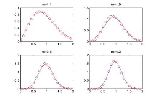
Figure 1: Nakagami-$m$ pdf marked by circles and its Rician approximation.

V Numerical Results

The results are plotted for unit mean power in both the desired and interfering channels. We assume identical and independent fading distribution in the desired and interferer links. The coverage probability plots for different fading distributions are provided in Fig. 2. To calculate coverage probability only a finite number of weights $N$ are required and are provided in Fig. 2. We observe that simulation results matches closely with the coverage probability derived. From the plots we can see that in $\kappa$-$\mu$ shadowed fading when $\kappa$ or $\mu$ or $m$ increases, coverage probability increases. From Fig. 3, we observe that the Rician approximation of Nakagami (which is used when $\mu$ is a non-integer) is very tight and the accuracy of approximate coverage probability increases with $\mathtt{SIR}$ threshold. As the exact coverage probability is not known when $\mu$ is a non-integer, we compute the squared error between the exact and approximate coverage probability when $\mu$ is an integer. As the coverage probability expressions involve multiple derivatives and summations, deriving an analytical upper bound on the approximation error is complicated. Hence in Fig. 4, we plot the squared error for different fading distributions. We observe that as the $\mathtt{SIR}$ threshold $T$ increases or with decrease in Nakagami fading or with decrease in $\kappa$, the squared error decreases and is also very low (order of $10^{-5}$).

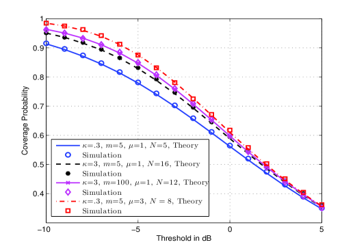
Figure 2: Theoretical and simulated coverage probability with $\kappa$-$\mu$ shadowed fading

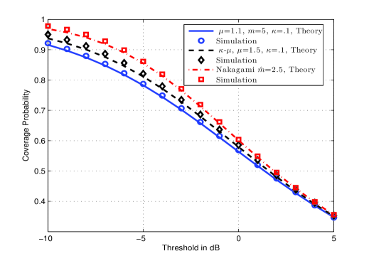
Figure 3: Theoretical and simulated coverage probability when $\mu$ is a non-integer. Nakagami-m fading of parameter $\hat{m}$ is a special case of $\kappa$-$\mu$ shadowed fading for $\mu$=$\hat{m}$, $\kappa\rightarrow 0$, $m\rightarrow\infty$ and $\kappa$-$\mu$ fading is a special case of $\kappa$-$\mu$ shadowed fading when $m\rightarrow\infty$

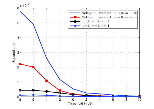
Figure 4: Squared error between exact and approximate coverage probability

VI Conclusion

In this paper, we have derived the coverage probability when both the desired and interfering links experience $\kappa$-$\mu$ shadowed fading. As $\kappa$-$\mu$ shadowed fading generalizes many popular fading distributions, the coverage probability expression derived can be used when the links experience Rician fading, Nakagami fading, Rician shadowing etc. which were hitherto unknown. By using a Rician approximation, we also derive an approximate coverage probability expression when parameter $\mu$ is not an integer. This is useful in deriving the coverage probability when the shape parameter of Nakagami fading is not an integer.

References

- [1] J. G. Andrews, F. Baccelli, R. K. Ganti “A tractable approach to coverage and rate in cellular networks,” IEEE Transactions On Communications, vol. 59, no. 11, pp. 3122-3134, November 2011.
- [2] H. S. Jo, Y. J. Sang, P. Xia, J. G. Andrews, “Heterogeneous cellular networks with flexible cell association: A comprehensive downlink SINR analysis,” IEEE Transactions on Wireless Communications, vol. 11, no. 10, pp. 3484-3495, October 2012.
- [3] H. S. Dhillon, M. Kountouris, J. G. Andrews, “Downlink MIMO HetNets: Modeling, ordering results and performance analysis,” IEEE Transactions on Wireless Communications, vol. 12, no. 10, pp. 5208-5222, October 2013.
- [4] X. Yang, A. O. Fapojuwo, “Coverage probability analysis of heterogeneous cellular networks in Rician/Rayleigh fading environments,” IEEE Communication Letters, vol. 19, no. 7, pp. 1197-1200, July 2015.
- [5] M. D. Renzo, P. Guan, “Stochastic geometry modeling of coverage and rate of cellular networks using the Gil-Pelaez inversion theorem,” IEEE Communication Letters, vol. 18, no. 9, pp. 1575-1578, September 2014.
- [6] P. Madhusudhanan, J. G. Restrepo, Y. Liu, T. X. Brown, “Analysis of downlink connectivity models in a heterogeneous cellular network via stochastic geometry,” IEEE Transactions on Wireless Communications, vol. 15, no. 6, pp. 3895-3907, June 2016.
- [7] M. D. Renzo, A. Guidotti, G. E. Corazza, “Average rate of downlink heterogeneous cellular networks over generalized fading channels : A stochastic geometry approach,” IEEE Transactions on Communications, vol. 61, no.7, pp. 3050-3071, July 2013.
- [8] A. Alammouri, H. ElSawy, A. S. Salem, M. D. Renzo, M. S. Alouini, “Modeling cellular networks in fading environments with dominant specular components,” arXiv:1602.03676, February 2016.
- [9] J. F. Paris, “Statistical characterization of - shadowed fading,” IEEE Transactions on Vehicular Technology, vol. 63, no. 2, pp. 518-526, February 2014.
- [10] L. M. Pozas, F. J. L. Martinez, J. F. Paris, E. M. Naya, “The - shadowed fading model : Unifying the - and - distributions,” to appear in IEEE Transactions on Vehicular Technology.
- [11] W. P. Johnson, “The curious history of Faà di Bruno’s formula,” The American mathematical monthly, vol. 109, no. 3, pp. 217-234, 2002.
- [12] A. Thummler, P. Buccholz, M. Telek, “A novel approach for phase-type fitting with the EM algorithm,” IEEE Transactions on Dependable and Secure Computing, vol. 3, no. 3, pp. 245-258, July 2006.
- [13] M. Nakagami, “The m-distribution-A general formula of intensity distribution of rapid fading,” Statistical Method of Radio Propagation, 1960.