See pages - of ParalogMatching_arxiv.pdf

SUPPLEMENTARY INFORMATION

1 Gaussian Direct Coupling Analysis

The basic steps for inferring contacts used in this work is the Direct Coupling Analysis (DCA) [1, 2, 3]. In this section, we recall the steps of inferring contact points, given an already matched multiple sequence alignment (MSA) $A$ of $M$ sequences of length $L$. Because the present work requires the statistical model to be re computed several times, we opted for the computationally fastest and simplest modeling, the Multivariate Gaussian Modeling (MGM) introduced in [4]

1.1 Notation

An MSA of $M$ sequences of length $L$ is represented by a $M\times L$ - dimensional array $A=\left(a_{i}^{m}\right)_{\,i\,=\,1,\,\ldots,\,L}^{\,m\,=\,1,\,\ldots,\,M}$, where $a$ belongs to an alphabet of $Q+1=21$ symbols corresponding to the $Q=20$ standard amino acids plus the “gap” symbol (-). We transform the MSA into a $M\times\left(Q\cdot L\right)$ - dimensional array $X=\left(x_{i}^{m}\right)_{i=1,\ldots,QL}^{m=1,\ldots,M}$ over a binary alphabet $\left\{0,1\right\}$ accounting for the occupation state of each residue position. Precisely, for $a=1,\dots,Q$ and $l=1,\dots,L$, $x_{\left(l-1\right)Q+a}^{m}:=1$ if the standard amino acid $a$ is present at residue position $l$, $x_{\left(l-1\right)Q+a}^{m}:=0$ otherwise. Notice that $x_{\left(l-1\right)Q+a}^{m}=0$ for all $a$ if the position $l$ corresponds to a gap ant that at most one of the $Q$ variables $x_{\left(l-1\right)Q+1}^{m},\dots,x_{\left(l-1\right)Q+Q}^{m}$ can be equal to one. We denote the row length of $X$ by $N:=QL$.

The empirical covariance matrix $C=\left(C_{nn^{\prime}}\right)_{n,n^{\prime}=1,\dots,N}$ associated do the data $X$ is defined by:

$$C_{nn^{\prime}}:=\frac{1}{M}\sum_{m=1}^{M}\left(x_{n}^{m}-\bar{x}_{n}\right)\left(x_{n^{\prime}}^{m}-\bar{x}_{n^{\prime}}\right)$$ (1)

where $\bar{x}_{n}:=\frac{1}{M}\sum_{m=1}^{M}x_{n}^{m}$ is the empirical mean. We collect empirical means into the vector $\bar{x}=\left(\bar{x}_{n}\right)_{n=1,\dots,N}$.

Within the multivariate Gaussian model with normal-inverse-Wishart prior introduced in Ref. [4], the maximum a posteriori (MAP) estimation of the model mean $\mu$ is simply equal to:

$$\mu:=(1-\lambda)\bar{x}+\lambda\eta$$ (2)

and for covariance matrix $\Sigma$, given by:

$$\Sigma:=\lambda U+\left(1-\lambda\right)C+\lambda\left(1-\lambda\right)\left(\bar{x}-\eta\right)^{T}\left(\bar{x}-\eta\right)$$ (3)

Here, $\lambda\in\left[0,1\right]$ is a parameter determining the relative strength of the prior, which we call “pseudocount” and which we typically set to the value $0.5$. The vector $\eta$ and the matrix $U$ are the prior estimators of the mean and the covariances, respectively. We take $\eta$ to be a uniform row vector of length $N$ with entries all equal to $\left(Q+1\right)^{-1}$, and $U$ to be a $N\times N$ - block-diagonal matrix composed of $Q\times Q$ blocks: the diagonal blocks have entries $Q\left(Q+1\right)^{-2}$ on the diagonal and $-\left(Q+1\right)^{-2}$ off-diagonal, while the off-diagonal blocks are set to $0$.

With these definitions, the logarithm of the MAP value (log-MAP in the following) for a multivariate Gaussian model is, up to an additive constant:

$$\mathcal{L}=-\frac{1}{2}\log\det\Sigma$$ (4)

We refer to Ref. [4] for details.

2 The Matching Problem

2.1 Matching definition

Assume two alignment arrays $X^{1}$ and $X^{2}$ are given, whose rows represent amino-acid sequences for two protein families in binary encoding. The number of columns of the two matrices is $N_{1}$ and $N_{2}$, respectively. We group the sequences (rows of the arrays) in $S$ contiguous chunks, such that all sequences within a group belong to the same species. At first, we assume that the number of sequences for any given species is the same for the two families. We denote by $M_{s}$ the number of sequences of the species $s$, so that $\sum_{s=1}^{S}M_{s}=M$. Setting $B_{1}:=0$ and $B_{s}:=\sum_{k=1}^{s-1}M_{k}$ if $S>1$, all rows corresponding to the species $s$ have indices in the interval $\mathcal{I}_{s}:=\left\{B_{s}+1,\dots,B_{s}+M_{s}\right\}.$

Our objective is to find the correct association between the sequences of the two families in each species by maximization of coevolution signals. Given our assumptions, this association is a matching between row $m$ of the array $X^{1}$ and a row $\pi\left(m\right)$ of the array $X^{2}$, $\pi$ being a permutation of the row indices of $X^{2}$ which preserves the species: $\pi\left(m\right)\in\mathcal{I}_{s}$ if $m\in\mathcal{I}_{s}$. We denote by $X^{2\pi}$ the array $X^{2}$ with rows permuted according to $\pi$, i.e. the elements of $X^{2\pi}$ are $\left(X^{2\pi}\right)_{mn}=X_{\pi\left(m\right)n}^{2}$. We also denote by $X^{\pi}$ the $M\times N$ - array, with $N:=N_{1}+N_{2}$, obtained by concatenating $X^{1}$ and $X^{2\pi}$. Finally, we define $C^{\pi}$, $\Sigma^{\pi}$ and $\mathcal{L}^{\pi}$ to be the empirical covariance matrix, MAP covariance matrix and log-MAP, respectively, associated to the concatenated data $X^{\pi}$ via the multivariate Gaussian model relations, eqs. (1), (3) and (4).

The two covariance matrices have a block structure:

$$C^{\pi} = \left[\begin{array}[]{c|c}C_{1}&D^{\pi}\\ \hline\cr\left(D^{\pi}\right)^{T}&C_{2}\end{array}\right]$$ (7)

$$\Sigma^{\pi} = \left[\begin{array}[]{c|c}\Sigma_{1}&\Phi^{\pi}\\ \hline\cr\left(\Phi^{\pi}\right)^{T}&\Sigma_{2}\end{array}\right]$$ (10)

$$(\Sigma^{-1})^{\pi} = \left[\begin{array}[]{c|c}\Sigma^{-1}_{1}&\Psi^{\pi}\\ \hline\cr\left(\Psi^{\pi}\right)^{T}&\Sigma^{-1}_{2}\end{array}\right]$$ (13)

The diagonal parts (of sizes $N_{1}\times N_{1}$ and $N_{2}\times N_{2}$) describe correlations within each protein, while the extra-diagonal blocks $D^{\pi}$ and $\Phi^{\pi}$ (of size $N_{1}\times N_{2}$), describe correlations (i.e. possible co-evolution) between the two proteins. The extra-diagonal blocks will then be the focus of our proposed matching strategies.

2.2 Scoring the matching

Our strategy for finding the best matching consists in maximizing some score within the multivariate Gaussian model for the joined families. From a Bayesian perspective, $\pi$ is an additional latent variable to infer, and one would ideally want to maximize the log-MAP of eq. (4), i.e. to find an optimal matching $\pi^{\star}$ defined as:

$$\pi^{\star}:=\arg\max_{\pi}\left(\mathcal{L}^{\pi}\right)$$ (14)

This is an arduous computational task: for realistic cases, the space search is huge (it grows faster than exponentially), $\mathcal{L}^{\pi}$ is rather costly to compute, and the landscape while varying $\pi$ is especially rugged, such that classic search strategies such as Simulated Annealing are infeasible. We thus resort to heuristic strategies, which have good performance in practice.

A first observation is that we can consider alternatives to the score function $\mathcal{L}^{\pi}$: according to the wisdom of co-evolution, pairs of interacting proteins should exhibit some co-evolution signals, encoded in both the covariance matrix $\Sigma^{\pi}$ and its inverse, the interaction matrix $J^{\pi}=-\left(\Sigma^{\pi}\right)^{-1}$. As their coefficients at $i$ and $j$ quantify the strength of coevolution between site $i$ and $j$, one could maximize some quantity involving $\Sigma^{\pi}$ or $J^{\pi}$. As the simplest choice, in the following we will consider the squared Frobenius norm of the off-diagonal MAP covariance, $\left\|\Phi^{\pi}\right\|_{F}^{2}=Tr\left(\left(\Phi^{\pi}\right)^{T}\Phi^{\pi}\right)$, as an additional scoring function, besides $\mathcal{L}^{\pi}$.

A second observation is that, as we shall show below, for both these scores we can devise a reasonably efficient hill climbing procedure: starting from some initial matching $\pi_{0}$, we produce a sequence of successive matchings $\pi_{1},\pi_{2},\dots$ by repeated application of a local optimization scheme, such that at each step the score that we are trying to maximize is (at least approximately) non-decreasing.

Finally, following the previous observation, we devised a strategy for obtaining a better matching by “mixing” two or more sub-optimal matchings.

In what follows, we detail the hill climbing procedure for the two score functions and the mixing procedure. These will form the building blocks of our overall heuristic strategies, which are explained in the following section.

2.2.1 Frobenius norm hill climbing

We first study the Frobenius norm score, defined as:

$$\left\|\Phi^{\pi}\right\|_{F}^{2} = Tr\left(\left(\Phi^{\pi}\right)^{T}\Phi^{\pi}\right)$$

$$= \sum_{n=1}^{N_{1}}\sum_{n^{\prime}=1}^{N_{2}}\left(\Phi_{nn^{\prime}}^{\pi}\right)^{2}$$

The basic idea is to derive the basic step of a hill climbing procedure as a local optimization process, in which one starts with a permutation $\pi$ and tries to find a similar permutation $\pi^{\prime}$ which maximizes the difference $\left\|\Phi^{\pi^{\prime}}\right\|_{F}^{2}-\left\|\Phi^{\pi}\right\|_{F}^{2}$. To simplify the notation, let us rewrite the expression for the extra-diagonal block of $\Sigma^{\pi}$ in eq. (3) as:

$$\Phi^{\pi}=\left(1-\lambda\right)D^{\pi}+L$$ (16)

so that we can write:

$$\left(\Phi_{nn^{\prime}}^{\pi^{\prime}}\right)^{2}-\left(\Phi_{nn^{\prime}}^{\pi}\right)^{2}=\left(1-\lambda\right)^{2}\left(\left(D_{nn^{\prime}}^{\pi^{\prime}}\right)^{2}-\left(D_{nn^{\prime}}^{\pi}\right)^{2}\right)+2\left(1-\lambda\right)\left(D_{nn^{\prime}}^{\pi^{\prime}}-D_{nn^{\prime}}^{\pi}\right)L_{nn^{\prime}}$$ (17)

We now focus on the first addendum; first, we define the matrices $Y^{1}$ and $Y^{2}$ obtained from $X^{1}$ and $X^{2}$ by subtracting their mean, such as their elements are, for $n\in\left\{1,\ldots,N^{1}\right\}$, $n^{\prime}\in\left\{1,\ldots,N^{2}\right\}$, $m\in\left\{1,\dots,M\right\}$:

$$Y_{mn}^{1} = X_{mn}^{1}-\bar{x}_{n}$$ (18)

$$Y_{mn^{\prime}}^{2} = X_{mn^{\prime}}^{2}-\bar{x}_{N^{1}+n^{\prime}}$$

With these, we can write eq. (1) as:

$$D_{nn^{\prime}}^{\pi}=\frac{1}{M}\sum_{m=1}^{M}Y_{mn}^{1}Y_{\pi\left(m\right)n^{\prime}}^{2}$$ (19)

and therefore

$$\left(O_{nn^{\prime}}^{\pi^{\prime}}\right)^{2}-\left(O_{nn^{\prime}}^{\pi}\right)^{2} = \frac{1}{M^{2}}\left(\left(\sum_{m=1}^{M}Y_{mn}^{1}Y_{\pi^{\prime}\left(m\right)n^{\prime}}^{2}\right)^{2}-\left(\sum_{m=1}^{M}Y_{mn}^{1}Y_{\pi\left(m\right)n^{\prime}}^{2}\right)^{2}\right)$$ (20)

We then restrict ourselves to permutations $\pi^{\prime}$ which only differ within a single species $s$ from $\pi$:

$$\pi\left(m\right)=\pi^{\prime}\left(m\right)\;\textrm{if}\>m\notin\mathcal{I}_{s}$$

and obtain:

$$\left(D_{nn^{\prime}}^{\pi^{\prime}}\right)^{2}-\left(D_{nn^{\prime}}^{\pi}\right)^{2} = \frac{2}{M^{2}}\sum_{m\in\mathcal{I}_{s}}\sum_{m^{\prime}\notin\mathcal{I}_{s}}Y_{mn}^{1}Y_{m^{\prime}n}^{1}\left(Y_{\pi^{\prime}\left(m\right)n^{\prime}}^{2}-Y_{\pi\left(m\right)n^{\prime}}^{2}\right)Y_{\pi\left(m^{\prime}\right)n^{\prime}}^{2}+$$ (21)

$$+\mathcal{O}\left(\left(\frac{M_{s}}{M}\right)^{2}\right)$$

$$D_{nn^{\prime}}^{\pi^{\prime}}-D_{nn^{\prime}}^{\pi}=\frac{1}{M}\sum_{m\in\mathcal{I}_{s}}Y_{mn}^{1}\left(Y_{\pi^{\prime}\left(m\right)n^{\prime}}^{2}-Y_{\pi\left(m\right)n^{\prime}}^{2}\right)$$ (22)

If we neglect the terms of order $\mathcal{O}\left(\left(\frac{M_{s}}{M}\right)^{2}\right)$, i.e. we assume that each single species has a few proteins compared with the size of the dataset, we can write:

$$\left\|\Phi^{\pi^{\prime}}\right\|_{F}^{2}-\left\|\Phi^{\pi}\right\|_{F}^{2} \propto \sum_{m\in\mathcal{I}_{s}}\sum_{n=1}^{N_{1}}\sum_{n^{\prime}=1}^{N_{2}}Y_{mn}^{1}\left(Y_{\pi^{\prime}\left(m\right)n^{\prime}}^{2}-Y_{\pi\left(m\right)n^{\prime}}^{2}\right)\left(\frac{\left(1-\lambda\right)}{M}\sum_{m^{\prime}\notin\mathcal{I}_{s}}Y_{m^{\prime}n}^{1}Y_{\pi\left(m^{\prime}\right)n^{\prime}}^{2}+L_{nn^{\prime}}\right)$$ (23)

$$= \sum_{m\in\mathcal{I}_{s}}\sum_{n=1}^{N_{1}}\sum_{n^{\prime}=1}^{N_{2}}Y_{mn}^{1}\left(Y_{\pi^{\prime}\left(m\right)n^{\prime}}^{2}-Y_{\pi\left(m\right)n^{\prime}}^{2}\right)\left(\Phi_{nn^{\prime}}^{\pi}-\frac{1}{M}\sum_{m^{\prime}\in\mathcal{I}_{s}}Y_{m^{\prime}n}^{1}Y_{\pi\left(m^{\prime}\right)n^{\prime}}^{2}\right)$$

$$= -\sum_{m\in\mathcal{I}_{s}}\mathcal{M}_{m\pi^{\prime}\left(m\right)}^{\pi,s}+\mathcal{A}^{\pi}$$

where in the last step we defined $\mathcal{A}^{\pi}$, which does not depend on $\mathscr{\pi^{\prime}}$and is therefore irrelevant for our optimization problem, and the cost matrix

$$\mathcal{M}_{mm^{\prime}}^{\pi,k} = -\sum_{n=1}^{N_{1}}\sum_{n^{\prime}=1}^{N_{2}}Y_{mn}^{1}\left(\Phi_{nn^{\prime}}^{\pi}-\frac{1}{M}\sum_{m^{\prime\prime}\in\mathcal{I}_{s}}Y_{m^{\prime\prime}n}^{1}Y_{\pi\left(m^{\prime\prime}\right)n^{\prime}}^{2}\right)Y_{m^{\prime}n^{\prime}}^{2}$$ (24)

Equation (23) has the form of a matching problem: we have an $M_{s}\times M_{s}$ cost matrix $\mathcal{M}^{\pi,s}$ and we want to find an optimal matching between the rows and the columns indices, such that the sum of the costs is minimal (and therefore the step in the Frobenius norm from $\pi$ to $\pi^{\prime}$ is maximal). This problem is computationally easy and can be solved very efficiently (e.g. via linear programming), in particular for small $M_{s}$.

Therefore, if we start from any permutation $\pi$, we can derive a new permutation $\pi^{\prime}$ by choosing a species $s$ and solving a small matching problem; the new permutation will only differ on the $s$-th block, and will likely have a bigger Frobenius norm, and can serve as basis for further iterations. We call this algorithm “Frobenius norm hill climbing”. The computation can be done reasonably efficiently as it only requires linear algebra operations and solving small matching problems; furthermore, in practice we only compute the matrices $\mathcal{M}^{\pi,s}$ once for the whole dataset at each iteration, after which we use them to update all the blocks independently in parallel, and use the new permutation to compute new matrices $\mathcal{M}^{\pi^{\prime},s}$ and so on. This parallel method of update is not only useful to save some computational time, but proves better in practice as a way to avoid fixed points in the iterative algorithm. A pseudocode for this procedure is shown in Algorithm 1.

The reason for using this algorithm is that it proved heuristically to be very fast and efficient in the early stages of the optimization, i.e. when starting from a random permutation, as will be discussed below.

Algorithm 1 FrobNormHillClimbing. This routine implements the Frobenius norm hill climbing algorithm derived in the text. Its arguments are the two alignment matrices minus the mean ($Y^{1}$ and $Y^{2}$ in the text, Y1 and Y2 here), the list of blocks indices ($\left\{\mathcal{I}_{s}\right\}_{s\in\left\{1,\ldots,S\right\}}$ in the text, Ilist here), an initial permutation ($\pi$ in the text, permutation here) and a group of parameters (pseudocount and iterations). It returns a new permutation ($\pi^{\prime}$ in the text, new_permutation here). Most auxiliary routines (e.g. num_columns, permute_rows) should have obvious meanings; compute_MAP_covariance implements eq. (3); permutation_by_matching calls some solver for the matching problem to obtain a permutation; multiplication (denoted by *) is intended to be matrix multiplication when matrices or vectors are involved; square brackets are used to denote elements of lists and submatrices (e.g.  Y1[I, {1,...,N1}], where I is a range, denotes a submatrix obtained by taking the rows I of the matrix Y1, and all of its columns).

function FrobNormHillClimbing(Y1, Y2, Ilist, permutation, pseudocount, iterations)

{

N1 = num_columns(Y1)

N2 = num_columns(Y2)

M = num_rows(Y1)

S = num_elements(Ilist) 

range1 = {1,...,N1}

range2 = {N1+1,...,N}

new_permutation = {1,...,M}

for iter = 1,...,iterations

{

Y2p = permute_rows(Y2, permutation)

Y = horizontal_concatenation(Y1, Y2p)

C = compute_MAP_covariance(Y, pseudocount)

Phi = C[range1, range2]

for s = 1,...,S

{

I = Ilist[s]

bY1 = Y1[I, {1,...,N1}]

bY2p = Y2p[I, {1,...,N2}]

T = Phi - ((1-pseudocount) * transpose(bY1) * bY2p) / M

COSTS = bY1 * T * transpose(bY2)

new_permutation[I] = permutation_by_matching(COSTS, I)

}

permutation = new_permutation

}

return new_permutation

}

2.2.2 Log-MAP hill climbing

Here, we perform a similar analysis to the one in the previous section for the log-MAP score $\mathcal{L}^{\pi}$: we consider two permutations $\pi$ and $\pi^{\prime}$, and we wish to some $\pi^{\prime}$ which maximizes the difference

$$\mathcal{L}^{\pi^{\prime}}-\mathcal{L}^{\pi} =- \frac{1}{2}\log\det\Sigma^{\pi^{\prime}}+\frac{1}{2}\log\det\Sigma^{\pi}$$ (25)

The concavity of the logarithm of the determinant of positive definite matrices ensures that:

$$\mathcal{L}^{\pi^{\prime}}-\mathcal{L}^{\pi} \geq- \frac{1}{2}\mathrm{Tr}\,\left(\Sigma^{\pi}\right)^{-1}\left(\Sigma^{\pi^{\prime}}-\Sigma^{\pi}\right)$$ (26)

therefore, we focus on minimizing only the term:

$$\mathrm{Tr}\,\left(\Sigma^{\pi}\right)^{-1}\left(\Sigma^{\pi^{\prime}}-\Sigma^{\pi}\right) = \lambda\left(\left(\Sigma^{\pi}\right)^{-1}\right)\left(C^{\pi^{\prime}}-C^{\pi}\right)$$ (27)

Again, this can be written as a matching problem:

$$\mathrm{Tr}\,\left(\Sigma^{\pi}\right)^{-1}\left(\Sigma^{\pi^{\prime}}-\Sigma^{\pi}\right) \propto \sum_{m=1}^{M}\mathcal{W}_{m\pi^{\prime}\left(m\right)}^{\pi}+\mathcal{B}^{\pi}$$ (28)

where $\mathcal{B}^{\pi}$ does not depend on $\pi^{\prime}$ and is therefore irrelevant, and the matching weights are encoded in the matrix:

$$\mathcal{W}^{\pi}=Y^{1}\Psi^{\pi}\left(Y^{2}\right)^{T}$$ (29)

where we recall (Eq.13) that $\Psi$ is the extra diagonal block of $\Sigma^{-1}$.

We are only interested in the diagonal blocks of the matrix $\mathcal{W}^{\pi}$, for which $m,m^{\prime}\in\mathcal{I}_{s}$ for some $s$, and we can perform the maximization independently and in parallel for each species block, as for the Frobenius norm case. In this way, we can define an iterative process which takes a given permutation $\pi$ as input and produces a new permutation $\pi^{\prime}$ such that $\mathcal{L}^{\pi^{\prime}}\geq\mathcal{L}^{\pi}$, and therefore produce a sequence of permutations with non-decreasing log-MAP. The pseudocode for this procedure, which is even more computationally efficient than the Frobeinus gradient ascent, is shown in Algorithm 2.

Unfortunately, our tests show that this algorithm, which we call “Log-MAP hill climbing”, is extremely prone to get trapped into fixed points. For this reason, we mostly use this method for refinement of solutions obtained by other means, since it typically does not provide big gains in terms of log-MAP (both in terms of gain-per-iteration and in terms of total gain up to the fixed point), even when starting from random initial permutations.

Algorithm 2 LogMAPHillClimbing. This routine implements the Log-MAP hill climbing algorithm derived in the text. It’s very similar to FrobNormHillClimbing (see Algorithm 1), but runs until a fixed point is reached.

function LogMAPHillClimbing(Y1, Y2, Ilist, permutation, psudocount)

{

N1 = num_columns(Y1)

N2 = num_columns(Y2)

M = num_rows(Y1)

S = num_elements(Ilist) 

range1 = {1,...,N1}

range2 = {N1+1,...,N}

new_permutation = {1,...,M}

fixed_point = false

while fixed_point == false

{

Y2p = permute_rows(Y2, permutation)

Yp = horizontal_concatenation(Y1, Y2p)

C = compute_MAP_covariance(Yp, pseudocount)

invC = inverse(C)

invPhi = invC[range1, range2]

for s = 1,...,S

{

I = Ilist[s]

bY1 = Y1[I, {1,...,N1}]

bY2 = Y2[I, {1,...,N2}]

COSTS = bY1 * invPhi * transpose(bY2)

block_permutation = permutation_by_matching(COSTS, I)

new_permutation[I] = block_permutation

}

if new_permutation == permutation

{

fixed_point = true

}

permutation = new_permutation

}

return new_permutation

}

2.2.3 Mixing local optima

As we mentioned above, the log-MAP hill climbing strategy shows a strong tendency to get stuck in local maxima. Supposing that we have obtained two different matchings $\pi_{1}$ and $\pi_{2}$ in such way, e.g. by initializing the algorithm from different initial random configurations, a simple and effective way to improve over these solutions is to obtain a new permutation $\pi^{\prime}$ by solving again the matching problem defined by eq. (28), in which however the matching weight matrix is obtained by

$$\mathcal{W}=\frac{1}{2}\left(\mathcal{W}^{\pi_{1}}+\mathcal{\mathcal{W}}^{\pi_{2}}\right)$$

where the weights $\mathcal{W}^{\pi_{1}}$ and $\mathcal{W}^{\pi_{2}}$ are computed according to eq. (29). The new permutation can then be refined via Log-MAP hill climbing. The pseudocode for this procedure is shown in Algorithm 3

This algorithm is generalizable in a number of ways (e.g. we could mix more than two solutions, tune the relative weights according to the associated Log-MAP, etc.), but our empirical tests show that using two permutations at a time seems to be the most effective approach.

Algorithm 3 MixPermutations. This routine implements the algorithm for mixing two permutations presented in the text. It’s very similar to LogMAPHillClimbing (see Algorithm 2), but takes two input permutations ($\pi_{1}$ and $\pi_{2}$ in the text, p1 and p2 here), and returns only one.

function MixPermutations(Y1, Y2, Ilist, p1, p2, pseudocount)

{

N1 = num_columns(Y1)

N2 = num_columns(Y2)

M = num_rows(Y1)

S = num_elements(Ilist) 

range1 = {1,...,N1}

range2 = {N1+1,...,N}

Y2p1 = permute_rows(Y2, p1)

Y2p2 = permute_rows(Y2, p2)

Yp1 = horizontal_concatenation(Y1, Y2p1)

Yp2 = horizontal_concatenation(Y1, Y2p2)

C1 = compute_MAP_covariance(Yp1, pseudocount)

C2 = compute_MAP_covariance(Yp2, pseudocount)

invC1 = inverse(C1)

invC2 = inverse(C2)

invPhi1 = invC1[range1, range2]

invPhi2 = invC2[range1, range2]

invPhiMix = (invPhi1 + invPhi2) / 2

new_permutation = {1,...,M}

for k = 1,...,S

{

I = Ilist[k]

bY1 = Y1[I, {1,...,N1}]

bY2 = Y2[I, {1,...,N2}]

COSTS = bY1 * invPhiMix * transpose(bY2)

block_permutation = permutation_by_matching(COSTS, I)

new_permutation[I] = block_permutation

}

return new_permutation

}

3 Computational strategies

We introduced the basic strategies for maximizing the two scoring functions and mixing different sub-optimal solutions. We now outline two different computational strategies for maximizing globally the permutation $\pi$. We start first by outlining the Iterative Paralog Matching, our most accurate strategy with larger computational complexity. Then, we outline the progressive paralog matching strategy, which turns out to be marginally less accurate then the Iterative Paralog Matching, but with a much lower computational complexity.

3.1 Iterative Paralog Matching

We describe here the complete Iterative Paralog Matching which we used to derive the results presented in the main text. It uses all three computational building blocks of the previous section; as an additional, final heuristic pass, it also employs a refinement aimed once again at escaping local maxima.

The protocol starting point is the generation of a large number of random permutations. Each of those is then used as a starting point for a Frobenius norm hill climbing phase. These are all independent and thus can be run in parallel. The number of iterations during this phase is a parameter of the protocol; we observed that in practice a plateau is typically reached after about $10$ iterations. In the following phase, we perform log-MAP hill climbing up to a fixed point (which is normally reached in a short number of iterations), again in parallel and independently for each configuration. After this, we collect all these configurations in a set, and we rank them according to their log-MAP score. We then apply this procedure iteratively: we take the two lowest-ranking configurations, removing them from the set; we mix them as described above, and obtain a new (typically better then both) configuration; we add this new configuration to the set. This phase continues until there is only one configuration left. In the final phase, we try to optimize futher this result by the following procedure: given a configuration, we produce a number (e.g. 32) of partially scrambled versions of it, and then we mix them progressively as in the previous phase, until we end up again with a single configuration. The scrambling is performed in this way: we fix a fraction (e.g. 50%) of all the matching indices, and randomize the rest while keeping the condition that interactions are only allowed within each species. This procedure is intended to escape from local maxima, and is iterated until it is judged that it is no longer effective (in our tests, this happened after $100$ to $200$ iterations).

Of course, this protocol can be improved in many ways. In fact, we also developed a simpler, trivially parallelizable and incremental version, in which the final phase is avoided and the mixing is performed by taking random pairs of configurations (thus avoiding the ranking). This protocol had similar performances in terms of the maximum value of the log-MAP that it was able to reach, at the cost of requiring a much larger number of initial configurations to start with.

A simplified pseudo-code for our protocol is shown in 4.

Algorithm 4 FindAlignment. This algorithm implements the complete optimization protocol described in the text. Its arguments are the two alignment matrices minus the mean ($Y^{1}$ and $Y^{2}$ in the text, Y1 and Y2 here), the list of blocks indices ($\left\{\mathcal{I}_{s}\right\}_{s\in\left\{1,\ldots,S\right\}}$ in the text, Ilist here), a number of permutations to start with (num_initial_permutations), a number of permutations to use in the last phase (num_scrambled_permutations), and some parameters (pseudocount, frob_iterations, final_phase_iterations, scrambling fraction). It calls FrobGradientAscent (see Algorithm 1) to bootstrap from random iterations and then iteratively mixes pairs of permutations with MixPermutations (see Algorithm 2) according to their ranking (auxiliary function mix_permlist_ranked, defined here) until only one permutation remains. The final pass scrambles the permutation, producing a new list which is then reduced again via mixing. LogMAPGradientAscent (see Algorithm 3) is used as a refinement after each step.

function FindAlignment(Y1, Y2, Ilist, num_initial_permutations, num_scrambled_permutations,

pseudocount, frob_iterations, final_phase_iterations,

scrambling_fraction)

{

perm_list = generate_random_permutations(num_initial_permutations, Ilist)

for i = 1,...,num_elements(perm_list)

{

new_perm = FrobGradientAscent(Y1, Y2, Ilist, permlist[i], pseudocount, iterations)

new_perm = LogMAPGradientAscent(Y1, Y2, Ilist, new_perm, pseudocount)

perm_list[i] = new_perm

}

final_perm = mix_permlist_ranked(Y1, Y2, Ilist, permlist, pseudocount)

for t = 1,...,final_phase_iterations

{

perm_list = generate_scrambled_perms(final_perm, num_scrambled_perms, scrambling_fraction)

final_perm = mix_permlist_ranked(Y1, Y2, Ilist, permlist, pseudocount)

}

return final_perm

}

function mix_permlist_ranked(Y1, Y2, Ilist, permlist, pseudocount)

{

while num_elements(perm_list) > 1

{

perm_list = sort_by_logMAP(perm_list, Y1, Y2, pseudocount)

p1 = perm_list[end]

p2 = perm_list[end-1]

new_perm = MixPermutations(Y1, Y2, Ilist, p1, p2, pseudocount)

new_perm = LogMAPGradientAscent(Y1, Y2, Ilist, new_perm, pseudocount)

perm_list[end-1] = new_perm

perm_list = drop_last_element(perm_list)

}

return perm_list[1]

}

3.2 Progressive Paralog Matching

The Iterative Paralog Matching outlined in Section 3.1, as discussed in the main text, turns out to be extremely accurate in terms of reproducing the correct matching on the two-component system biological dataset. However, due to computational complexity issues, it hardly scales for genome-wide analysis. To overcome such limitation, we propose a faster and simpler heuristic strategy: the Progressive Paralog Matching.

Due to the size of the matching space, we propose a step-by-step inference strategy by including larger and larger chunks (i.e. block of species) to the alignments to be matched. To proceed recursively, we need to single out, at each step, the matching with the greatest likelihood, employing an Maximum A Posteriori Estimator (MAP). The criterion to select a given species $s$ is the entropy $\omega_{s}$, defined as the log of the number of possible matchings of homologs within this genome. Considering now the general case in which the species sizes can be different for different families, we denote by $M_{s}^{1}$ (resp. $M_{s}^{2}$) the number of protein sequences in species $s$ found in the alignment of protein family $\mathcal{F}_{1}$ (resp. $\mathcal{F}_{2}$). Assuming, for example, that $M_{s}^{1}>M_{s}^{2}$:

$$\omega_{s}=\log\left(\frac{M_{s}^{1}!}{\left(M_{s}^{1}-M_{s}^{2}+1\right)!}\right)$$ (30)

We are going to denote $X^{\omega}$ and $C^{\omega}$ the data and correlation matrices obtained by matching all species $s$ characterized by an entropy $\omega_{s}\leq\omega$.

Initialization step: Genomes readily matched by uniqueness ($M_{s}^{1}=M_{s}^{2}=1$), have an entropy $\omega_{s}=0$ and therefore provide a natural initialization $X^{0},C^{0},\Sigma^{0}$.

Propagation step: We then proceed recursively. We assume that the matching is known for species up to entropy less than or equal to $\omega$. The model inferred given that matching has parameters $(\mu,\Sigma)$. We consider the next species, say $q$, of entropy immediately above $\omega$, $\omega_{q}>\omega$. The set of sequences in $q$ defines two sub-MSA for family $1$ and $2$, $X^{1}$ and $X^{2}$. As explained in Sec.2.1, a matching $\pi$ is defined as a concatenation of $X^{2}$ on $X^{1}$. We denote by $X^{\pi}$ the full, concatenated, MSA.

$X^{\pi}$ having a small number of rows w.r.t the whole dataset, it only slightly perturbs the empirical correlation matrix $C^{\pi}=C+\Delta C$, and similarly $\Sigma^{\pi}=\Sigma+\Delta\Sigma$ from Eq.3. At this point, the same reasoning presented in Sec.2.2.2 can be used. More precisely, one can score the best sub-matching $\pi$ for species $q$ by evaluating the score matrix:

$$\mathcal{W}=\left(X^{1}-\mu^{1}\right)\Psi^{-1}\left(X^{2}-\mu^{2}\right)^{T}\\$$ (31)

with $\mu^{1}$ ($\mu^{2}$) respectively the $N_{1}$ first (the $N_{2}$ last) components of the mean vector $\mu$, and $\Psi$ the extra-diagonal block of $\Sigma^{-1}$ (Eq.13). Once the cost matrix is computed, the best matching $\pi$ can be recovered by standard linear programming. The newly matched species $q$ is added to the pool of known species, and the new model parameters $(\mu,\Sigma)$ recomputed by adding the block $X^{\pi}$ to $X^{\omega}$.

The above step is repeated until the full alignment is matched. This algorithm is very scalable, as it runs over an alignment of $20000$ sequences in less than $10$ minutes, on a laptop (implementation in Julia).

3.3 Contact Map Predictions and PPI DCA Scoring

All contact predictions presented in the Main Text, such as Fig.2, 3 and 4 are done by Pseudo-Likelihood Maximization [5], using the Julia Package (github.com/pagnani/PlmDCA) with default parameters.

The scoring of the interactions between the Tryptophan proteins as presented in Fig.4 was done using the procedure described in [6]: we ranked the inter-protein scores from the largest, and consider the mean over the $4$ largest. We also checked other scores found in the literature [7]; they do not change the conclusion of the study.

4 Statistics Tables about the Tryptophan Dataset

The following table contains various statistics about the set of Tryptophan alignments used to assess the interaction network. The set is made of seven proteins, labelled from A to G. Table S1 contains information about the single proteins. Instead, Table S2 contains the statistics of resulting matched pairs of alignments using various methods: uniqueness, genetic or from co-evolution. Finally, Figs.S1 and S2 present a more complete overview of the paralogs statistics of this dataset.

	L	M	P	S	Quartiles
TrpA	259	10220	4.457	32.604	(1.0,1.0,2.0)
TrpB	399	46557	16.992	145.826	(3.0,4.0,6.0)
TrpC	254	10323	4.536	39.868	(1.0,1.0,1.0)
TrpD	337	17582	7.130	59.693	(1.0,2.0,2.0)
TrpE	460	28173	11.749	124.933	(2.0,3.0,4.0)
TrpF	197	8713	4.122	32.400	(1.0,1.0,1.0)
TrpG	192	78265	24.713	187.331	(5.0,7.0,9.0)

Table S1: For each protein in the Tryptophan Operon, the size of the protein $L$, the total number of sequences $M$ in the alignments. $P$ indicates the average number of paralogs per species and $S$ the standard deviation. Finally, the three quartiles, in order, are presented in the last column. More details are given in Fig.S1.

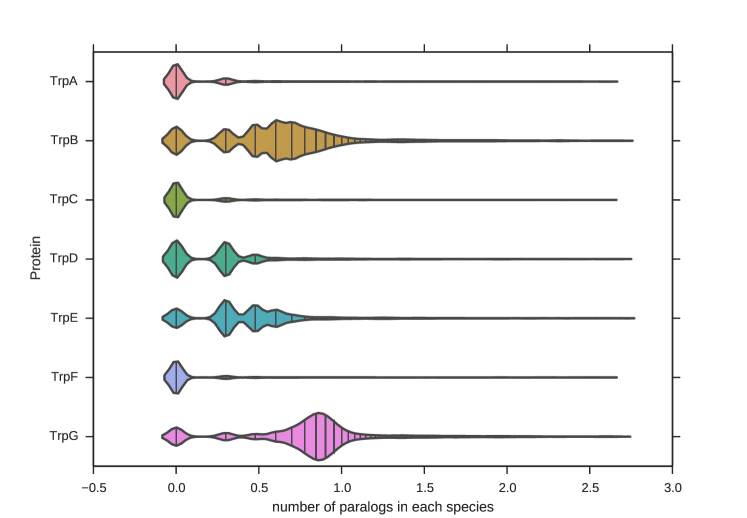
Figure S1: The distribution of the log10 number of paralogs in species, for each Trp protein. A cut-off at a maximum of $500$ paralogs by species has been chosen for plotting convenience. The sticks represent the boxes of the histogram used to generate the smooth violin plot. The elongated structures come from few species that present a very high number (greater than $100$) of paralogs.

		unique	genetic	covariation	score
TrpA	TrpB	95	4374	4915	0.337
TrpA	TrpC	1546	3198	6255	0.137
TrpA	TrpD	743	2823	6188	0.121
TrpA	TrpE	247	3118	5285	0.115
TrpA	TrpF	1433	3357	5701	0.139
TrpA	TrpG	22	4646	4176	0.118
TrpB	TrpC	82	3326	4425	0.145
TrpB	TrpD	95	3737	7242	0.112
TrpB	TrpE	51	3911	10720	0.096
TrpB	TrpF	95	3643	4064	0.137
TrpB	TrpG	41	8053	16437	0.090
TrpC	TrpD	748	3392	5778	0.129
TrpC	TrpE	256	2976	4839	0.127
TrpC	TrpF	1578	3825	5811	0.135
TrpC	TrpG	18	4272	3827	0.135
TrpD	TrpE	156	2681	7469	0.100
TrpD	TrpF	695	2819	5165	0.149
TrpD	TrpG	28	6249	6450	0.129
TrpE	TrpF	240	2519	4295	0.113
TrpE	TrpG	15	5324	9796	0.245
TrpF	TrpG	32	3635	3457	0.126

Table S2: For all possible pairings of proteins, the resulting size of the concatenated MSA, following various matching procedures: unique for matched by uniqueness; genetic for matched by genetic distance; covariation for matched by co-evolution analysis. score is the score obtained from the alignments matched by co-evolution analysis, as presented in [6].

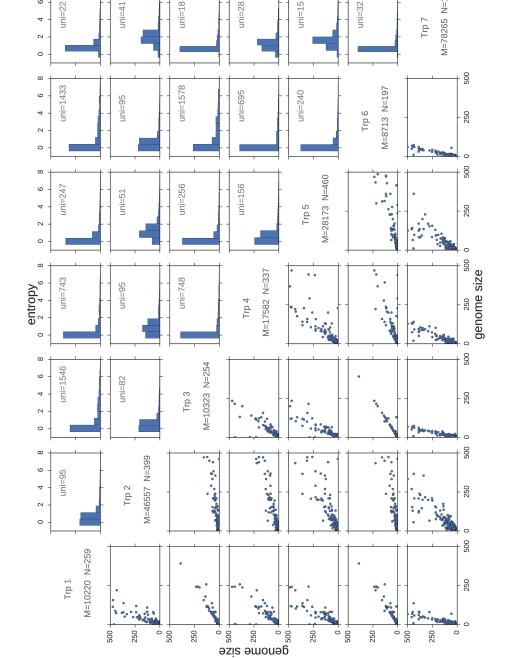
Figure S2: Table of histograms. The above triangular part represents the histogram of the entropies of the species, as given Eq.30. $uni$ is the size of the matched by uniqueness alignments. The diagonal part recalls the statistics presented in Table.S1. Finally the lower triangular part are scatter plots: each point represents a particular species, with its coordinates as the number of paralogs for each protein. A cut-off of $500$ paralogs by species has been chosen for plotting convenience.

References

- [1] Martin Weigt, Robert A. White, Hendrik Szurmant, James A. Hoch, and Terence Hwa. Identification of direct residue contacts in protein-protein interaction by message passing. Poc. Natl. Acad. Sci., 106(1):67–72, 2009.
- [2] Debora S. Marks, Lucy J. Colwell, Robert Sheridan, Thomas A. Hopf, Andrea Pagnani, Riccardo Zecchina, and Chris Sander. Protein 3d structure computed from evolutionary sequence variation. PLoS ONE, 6(12):e28766, 12 2011.
- [3] Faruck Morcos, Andrea Pagnani, Bryan Lunt, Arianna Bertolino, Debora S Marks, Chris Sander, Riccardo Zecchina, José N Onuchic, Terence Hwa, and Martin Weigt. Direct-coupling analysis of residue coevolution captures native contacts across many protein families. Poc. Natl. Acad. Sci., 108(49):E1293–E1301, 2011.
- [4] Carlo Baldassi, Marco Zamparo, Christoph Feinauer, Andrea Procaccini, Riccardo Zecchina, Martin Weigt, and Andrea Pagnani. Fast and accurate multivariate gaussian modeling of protein families: Predicting residue contacts and protein-interaction partners. PLoS ONE, 9(3):e92721, 2014.
- [5] Magnus Ekeberg, Cecilia Lövkvist, Yueheng Lan, Martin Weigt, and Erik Aurell. Improved contact prediction in proteins: Using pseudolikelihoods to infer potts models. Phys. Rev. E, 87:012707, Jan 2013.
- [6] Christoph Feinauer, Hendrik Szurmant, Martin Weigt, and Andrea Pagnani. Inter-protein sequence co-evolution predicts known physical interactions in bacterial ribosomes and the trp operon. PLoS ONE, 11(2):1–18, 02 2016.
- [7] Sergey Ovchinnikov, Hetunandan Kamisetty, and David Baker. Robust and accurate prediction of residue–residue interactions across protein interfaces using evolutionary information. eLife, 3, 2014.